Article

Assessing Climate Change Impacts on Streamflow, Sediment and Nutrient Loadings of the Minija River (Lithuania): A Hillslope Watershed Discretization Application with High-Resolution Spatial Inputs

1
Marine Research Institute, Klaipeda University, 92294 Klaipeda, Lithuania
2
ISMAR-CNR, Institute of Marine Sciences, 30122 Venezia, Italy
3
Department of Inland Water Resources and Management, Faculty of Aquatic Sciences, Istanbul University, 34134 Istanbul, Turkey
*
Author to whom correspondence should be addressed.
Water 2019, 11(4), 676; https://doi.org/10.3390/w11040676
Submission received: 5 February 2019 / Revised: 26 March 2019 / Accepted: 28 March 2019 / Published: 1 April 2019
(This article belongs to the Special Issue Diffuse Water Pollution)

Abstract

:
In this paper we focus on the model setup scheme for medium-size watershed with high resolution, multi-site calibration, and present results on the possible changes of the Minija River in flow, sediment load, total nitrogen (TN), and total phosphorus (TP) load in the near-term (up to 2050) and long-term (up to 2099) in the light of climate change (RCP 4.5 and RCP 8.5 scenarios) under business-as-usual conditions. The SWAT model for the Minija River basin was setup by using the developed Matlab (SWAT-LAB) scripts for a highly customized watershed configuration that addresses the specific needs of the project objective. We performed the watershed delineation by combining sub-basin and hillslope discretization schemes. We defined the HRUs by aggregating the topographic, land use, soil, and administrative unit features of the area. A multisite manual calibration approach was adopted to calibrate and validate the model, achieving good to satisfactory results across different sub-basins of the area for flow, sediments and nutrient loads (TP and TN). After completing the climate change scenario calculations, we found that a net decrease of flow (up to 35%), TN (up to 34%), and TP (up to 50%) loads are projected under both scenarios. Furthermore, we explored the changes in the streamflow composition and provide new insight on the reason of projected nutrient load decrease.

Graphical Abstract

1. Introduction

The recent State of the Baltic Sea report [1] shows that more than 97% of the Baltic Sea area suffers from eutrophication due to past and present excessive inputs of nitrogen and phosphorus. Owing to the implementation of the Baltic Sea Action Plan [2] by the Baltic Marine Environment Protection Commission (also known as Helsinki Commission, HELCOM) member states, the inputs from land have decreased considerably, but the effects of these measures are generally not yet reflected in the status. According to the assessment of progress towards the national targets for input of nutrients achieved by 2014 [3], Lithuania, as a HELCOM member, has yet to reduce the inputs to the maximum allowable levels, though the country has made some progress; for example, Lithuania was the only country that reduced total phosphorus inputs to all sub-basins to which it contributes [3].
Adaptation to climate change is a central issue for the planning and implementation of measures to reduce nutrient inputs, as well as for adjusting the level of nutrient input reductions to ensure protection of the Baltic Sea marine environment in a changing climate. Currently, the maximum allowable inputs are calculated under the assumption that the Baltic Sea environmental conditions are in a biogeochemical and physical steady-state [1], which is not likely to last with a changing climate.
Most of the land-based nutrient contribution from Lithuania to the Baltic Sea comes through the Nemunas River, which is the fourth largest river draining into the Baltic. The Nemunas watershed is shared by Belarus (48%), Lithuania (46%), Poland (2.57%), the Russian Federation Kaliningrad oblast (3.34%), and Latvia (0.09%) [4] (Figure 1), however, the responsibility to reduce the land-based nutrient loads to the river falls mainly on Lithuania, as Belarus is not a HELCOM nor an EU member, thus, is not bound by related international agreements.
Several studies conducted in the Baltic Sea region have addressed the effects of climate change on the river discharge at large scale [5,6,7] and medium to small scale [4,8,9], and studies focused on nutrient load change [10,11,12] from catchments in the Baltic Sea area. Some studies indicate that the current climate change trends for the region might result in an additional increase in the nutrient reduction targets [13]. This would mean that Lithuania needs to adapt and optimize land and fertilization management, nutrient recycling, rural water management, and implement other nutrient reduction and retention measures to achieve substantial progress for minimizing nutrient transport to the rivers, into the Curonian Lagoon and subsequently—to the Baltic Sea. Our conducted study aims to contribute to this effort by providing awareness of possible nutrient load changes in the light of climate change in the Nemunas River watershed. Furthermore, we intend to create a tool which will be flexible enough to simulate large-scale transboundary watershed level processes (hydrology, sediment, and nutrient load), for which course resolution data and model setup is sufficient; and regional, local, or even farm-scale management practices, for which a high-resolution model with adequate physical process representation in the watershed would be best suited.
We have tackled the challenges of creating a large-scale transboundary model for assessing the hydrological and water quality changes in a sub-basin of Nemunas watershed, located in Belarus (Vilija River basin) [14], which is the east most area of the entire watershed. Moving on with the study, now we tackle a similar challenge in the territory of Lithuania and the west-most area of the Nemunas River watershed, where the Minija River basin is situated (see Figure 1). In this paper we present the results of the model setup and test the watersheds response to climate change for near-term (up to 2050) and long-term (up to 2099) under the “business as usual” conditions with two Representative Concentration Pathways (RCP): RCP4.5 and RCP8.5, derived from Hadley Global Environment Model 2—Earth System (HadGEM2-ES) [15]. Located close to the coastal area, the created study and drawn conclusions may serve as a proxy to the entire coastal region of the East Baltic.
The Minija River basin model should be able to represent the study area and to simulate the hydrology and the water quality of the river and its response to different stressors, such as climate conditions. Furthermore, the model must be able to incorporate field-scale changes in the land use and land management; therefore, the model setup must reflect the processes in the sub-basin as accurately as possible. The SWAT (Soil and Water Assessment Tool) was chosen for this study for its comprehensive ability to simulate basically any type of hydrological model setup, which is backed-up by multiple application examples (all can be found in the SWAT publication database [16] and a general model description is available in Supplementary Material A). Although the standard geographic information system (GIS) tools for model setup (like ArcGIS, ESRI 2011. ArcGIS Desktop: Release 10. Redlands, CA: Environmental Systems Research Institute.) are commonly used, we found that they are preprogrammed to specific datasets to generate a default SWAT parametrization. Some allow the usage of a lookup table for different and non-standard pixel values in user-supplied grids; however, the SWAT database table integrated into those user interfaces cause some limitations and are not always easy to extend. Thus, we chose to use the developed script-based SWAT input generator coded in MATLAB (The MathWorks, Inc., Natick, Massachusetts, United States): SWAT-LAB (N. Čerkasova, Klaipėda, Lithuania [14]). The benefits of the script-based input generator are the flexibility in terms of automatic data generation, support of any type of model discretization (sub-basin, hillslope, or grid [17]), no limitation on the model complexity and others [14]. Using SWAT-LAB we could create a non-standard model setup which represents the spatial relationships of objects within the Minija watershed closest to the real physical conditions.

2. Materials and Methods

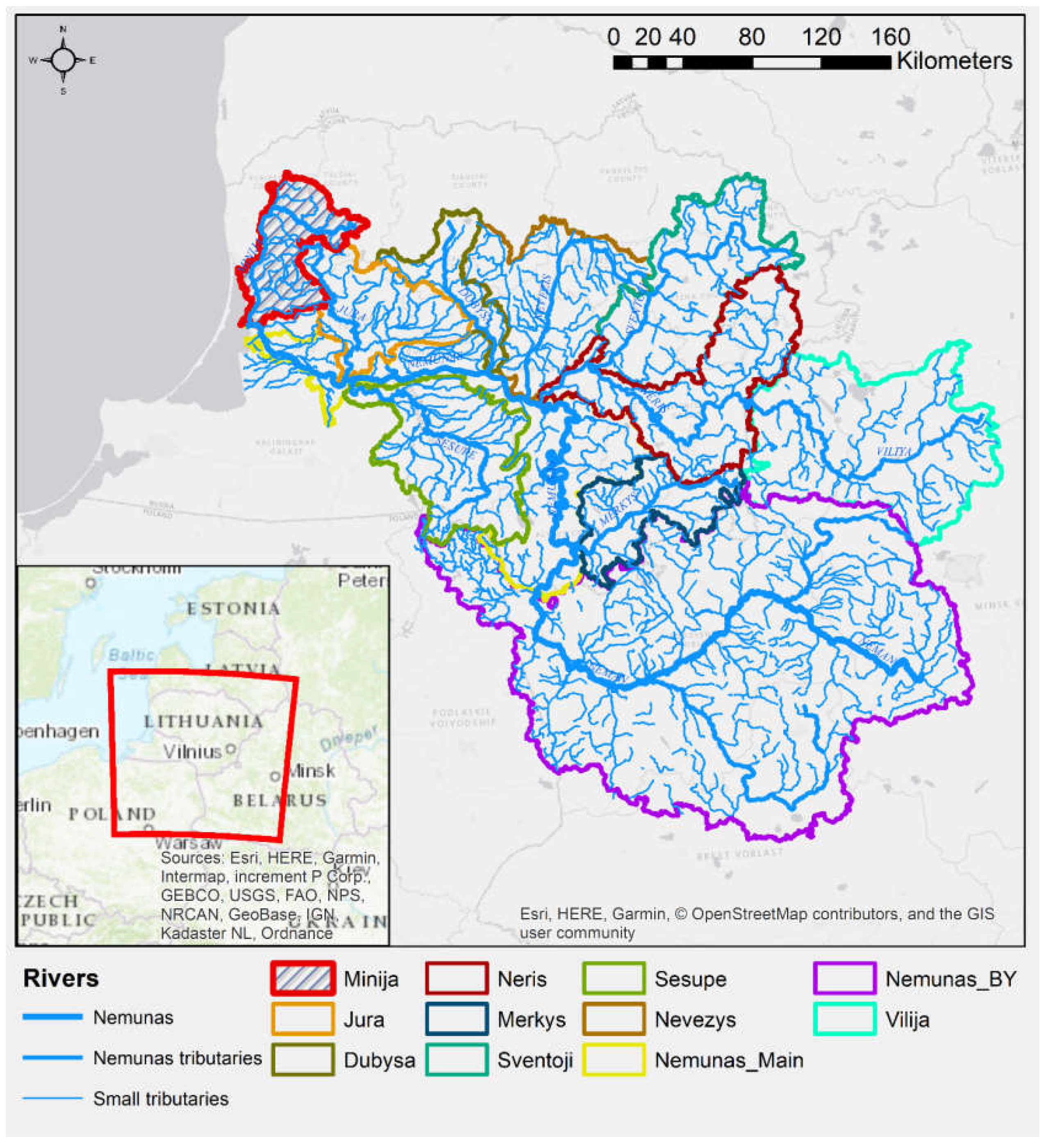
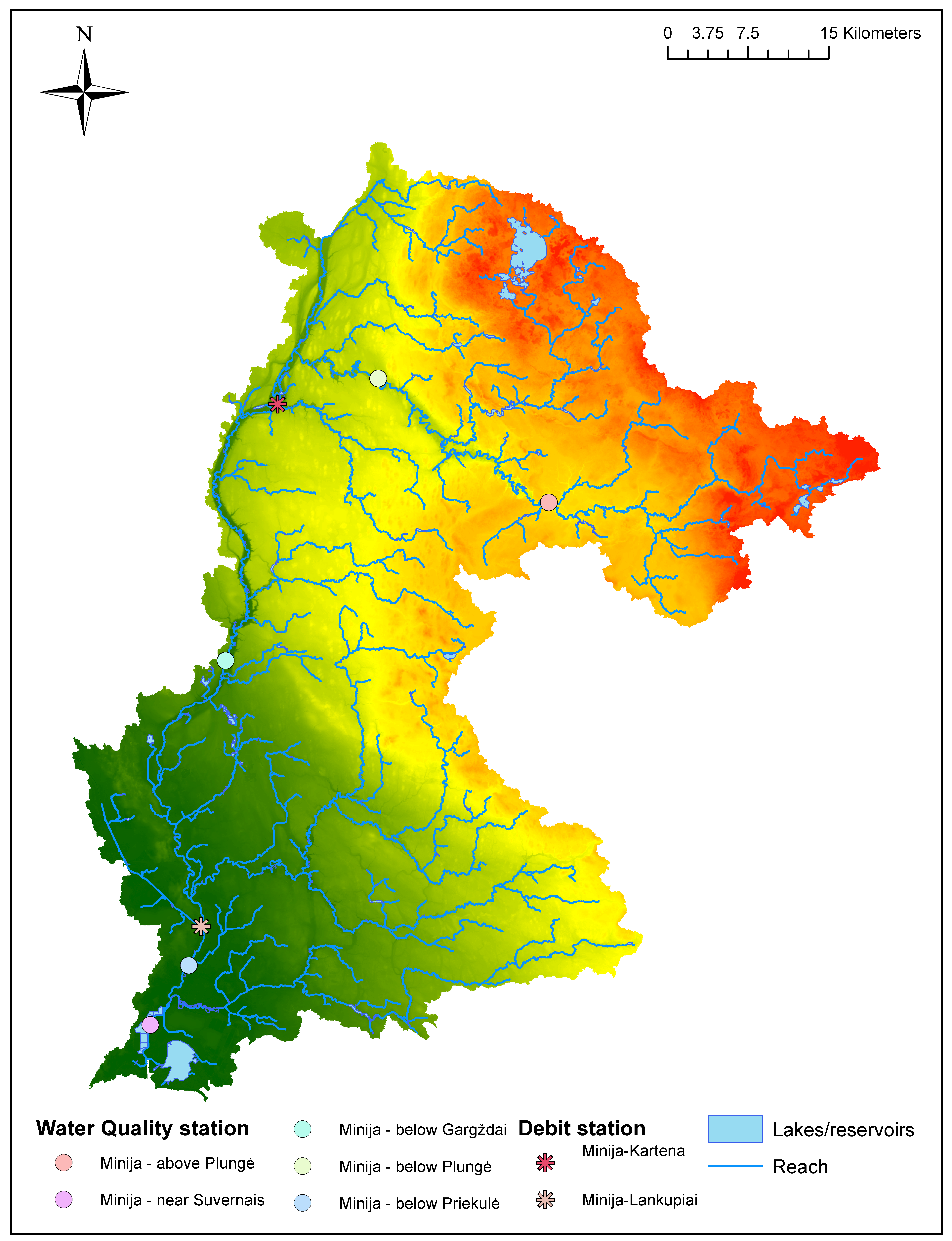
2.1. Case Study Description

The Minija River basin is situated in the west of Lithuania; positioned close to the coastal region and is a part of the Curonian Lagoon drainage basin (Figure 1). The Minija River’s length is 201.8 km, its watershed area is 3097.04 km2 with an annual average discharge of 38.7 m3/s [18]. Minija discharges into the Nemunas River at the very mouth, so it is a direct contributor to the flow, nutrient, sediment and bacteria to the Curonian Lagoon [19]. A number of protected areas are established and are a part of the river basin, such as the Samogitia National Park (Žemaitija National Park), Salantai Regional Park, Nemunas Delta Regional Park (which is a Ramsar site), and the Minija River Ichthyological Reserve. The river basin is under stress from different sources of pollution, including agriculture and aquaculture, recreational activities, domestic and industrial wastewater and others.
The Minija River basin is located in the lowland, mainly flat zone (Figure 2a,b). Winter pasture, followed by forests and agricultural regions, dominates the land use of the area (Figure 2c). This lets us assume that the major part of the pollution is coming from diffused sources. On the other hand, the agriculture and animal handling in the protected areas are strongly regulated by regional law, i.e., the number of livestock per hectare is limited, and thus this source of pollution might be of less influence than in other regions.
Located in the post-glacial area, the soils of the watershed are dominated by Hapli-Epihypogleyic Luvisol (IDg8-p), and generally by soils formed by fluvioglacial deposits, mainly sandy and loam deposits (JIb2, GLb2) [20] (Figure 2d). The delta region is dominated by wet alluvial soils, thus, the main land use of the low-lying area are polders.
The relation between the river discharge regime and the precipitation received by the watershed suggests that there are additional processes, which govern the streamflow and have a more significant impact than the surface runoff (Figure 3). Evapotranspiration (ET) has a great influence on the streamflow, although the case study area is situated in a temperate climate zone (or humid continental climate as defined by Köppen [21]). As can be seen in Figure 3, ET and rainfall alone cannot fully describe the streamflow intensity of the Minija River.
The river stream can be categorized as the gaining or effluent, meaning that there is an increase in discharge downstream and it depends on the water table, therefore, we suggest that the groundwater contribution to the stream has a significant influence in the watershed. Other studies have suggested that the air temperature, plant cover and activity, and evapotranspiration are the regulating factors that link precipitation and river flow [4] in the Nemunas River basin, which the Minija River is a part of. These discrepancies in various studies suggest that a more detailed analysis is needed on the composition of the stream flows of the entire Nemunas River basin to determine the most significant regulating factor of the discharge. Modelling studies, such as this, can help broaden the knowledge and understanding about the hydrological regime of rivers in the area.

2.2. Model Discretization Scheme

The Minija River basin model is a part of the larger modelling framework covering the entire Nemunas River watershed [14]. To build a high-resolution model for the entire watershed we split the basin into manageable sub-models, based on their location and the individual sub-watershed topology. Minija River model is the west-most part of this framework (see Figure 1).
The first step of model setup is the watershed discretization.
The standard discretization approach that is conducted by most of the SWAT users is HRU (hydrologic response unit)-based. In this approach it is assumed that the outflow from each HRU is equally routed to the watershed outlet. While it is often possible to produce results with similar modelling performance in terms of goodness of fit compared to more advanced discretization methods such as hillslope/catena or grid [22,23], an HRU-only-based discretization approach does not realistically link the cascade of flow and related impacts of it on the hydrographs and pollutographs [24]. Sub-basin HRU-based lumped models often respond less to changes in land use, soil, and weather conditions and need to be recalibrated with each changing scenario [24]. To counteract the lack of realism caused by discarding the natural pathways of unchannelized routing, Jencso et al, 2010; Kraf et al. (2012); Vigiak et al. (2015); Zao and Beighley (2016); Hoan et al. (2017) and Vigiak et al. (2017) [25,26,27,28,29,30] utilized the hillslope/catena approach, whereas Gorgan et al., (2012); Pignotti et al. (2017) [31,32] preferred the grid based discretization approach. If SWAT is operated following the grid-base discretization approach, each grid cell must be considered as a SWAT sub-basin resulting in increase of the computational burden and, therefore, the runtime orders of magnitude, depending on the grid resolution. Further details on the increase of runtime because of following the grid-based discretization option as applied in SWAT is discussed by Arnold et al. (2010) [22]. Drawing upon the experiences published previously, the optimum discretization method considering the realistic link of the cascade of flow and related impacts of it on the hydrographs and pollutographs and the computational burden of more advanced discretization methods, hillslope/catena-based discretion can be considered as the optimum.
The ideas related to best management practices for nutrient loads reduction published by Leh et al. (2008) [33] focused on field scale modelling, and Qin et al. (2018) [34] focused on spatial optimization approach to watersheds based on slope position units, we concluded that hillslope discretization is physically more realistic and will produce more accurate results, in case the model set-up in this study would be operated for simulations related to land use change and pollution prevention measures programs in the future. A recent research comparing different watershed configurations (HRUs, spatially explicit HRUs, hydrologically connected fields, and slope position units.) by Zhu et al. (2018) [35] also states that using the slope position units as BMP configuration units with the hillslope based discretization yielded the best results.
Another reason for implementing the hillslope discretization scheme in this study is that; the modelling tool SWAT used in this study is continuously revised and is now undergoing a new development cycle named SWAT Plus [36], which is the future SWAT. SWAT Plus, to which many previously models developed on SWAT, including the model setup in this study, would be ported to, relies on a better and more comprehensive landscape unit discretization, which includes more cascade-based routing, resembling the hillslope/catena discretization. Therefore, incorporating hillslope discretization into this study, is considered a better strategy for the easier port of the model developed presently into the future.
Modelling is an “alive” process. The Chesapeake Bay Watershed Model is a good example for this statement. As reported by Linker et al. (2002) [37], the modelling efforts began in 1982 and were continued as multiple phases, the first phase being initiated in 1985 and reaching Phase 5.3 in 2010 [38]. Recently, modelling phase 6 was initiated [39], which incorporates more detailed and revised input data and more advanced modelling tool and infrastructure ever. Considering the fact that model building is a time-costly effort, we believe that developing a model that would cover not only the aims of one study but more flexibly applicable to other future studies as much as possible within the resources made available for this study is the wiser roadmap to follow and therefore, we applied the hillslope based discretization to our model, considering its further use of land-use change and diffuse pollution measure scenarios, which are not covered in this study. However, all graphical user interface (GUI) tools developed for SWAT incorporate only the sub-basin/HRU discretization, which is the main reason why a script-based model setup approach was chosen for this study.
To take advantage of the model flexibility, we first divide the watershed into sub-basins using the topographical features of the area, and then we further divide the sub-basins into hillslopes, thus producing a hillslope discretization [17] (a thorough description of the procedure is available in the Supplementary Material B). Next, we use a modified HRU definition procedure and run SWAT-LAB [14] to produce HRUs from a unique combination of topography, slope, soil, land use, and administrative unit grids.
When defining the sub-basins in the Minija River model, we identified the main processes of interest and produced the following types of sub-basins:
  • Urban sub-basins (completely channelized);
  • Agricultural sub-basins (partly channelized);
  • Pond/reservoir sub-basins (completely channelized);
  • Forest/buffer sub-basins (not channelized);
  • Stream and forest sub-basins (partly channelized); and
  • Stream sub-basins (completely channelized).
These sub-basin types reflect the physical conditions in the study area.
As stated previously, one of the aims of the model design and developments can be considered as “to utilize for possible future studies”. Models are not only used for system analysis but also to answer the management questions for the governmental agencies. Lithuania is a part of the European Community, hence it is subjected to the European Water Framework Directive (WFD) [40]. The WFD established a legal framework to achieve sustainable water management in the EU. The WFD is implemented through six-year recurring cycles. Member States were required to deliver their first River Basin Management Plans by the end of 2009 and shall review these plans every six years. The Programmes of Measures developed under the plans had to be operational by the end of 2012. The 2nd cycle RBMPs needed to be in place by the end of 2015. By 2019, the WFD should be reviewed and, if necessary, revised. These facts imply that any watershed model would be facing to generate supporting information to answer more diverse and possibly more detailed management questions and should therefore be more flexible and more expandable and, if possible, should not be limited to single study aims. The model in this study, which is focused on the impact of climate change on the nutrient loads, is developed considering that it would be further utilized for land use change and best management practice scenarios in the future, which are not the aims of this study, however, components of which should be preemptively included into any model developed for the sake of “economy” in the efforts of watershed and water quality model development.

2.3. Addressing the Model Complexity

Dealing with the high-resolution spatial data of the DEM, soil and land use provided us with the possibility to create a very detailed model. However, the usability of this model had to be addressed. For large-scale applications, a coarse resolution model usually performs adequately for yearly or monthly flow/load predictions [41,42], but there is a general trend for the relative error to increase with the decrease of the spatial input data resolution, whilst the number of sub-watersheds needed for accurate predictions of sediment losses, has to increase [43]. The known solutions to deal with the SWAT model complexity during the setup is the use of coarse resolution data or reducing the number of HRUs by merging (i.e., merging all the HRUs beneath a given threshold with a dominant HRU, etc.). Alternatively, simplifying the input data (i.e., reclassifying the land use or soil maps or aggregating classes), therefore producing fewer HRUs, is also a solution.
Since the model will be used for both total seasonal and annual runoff and sediment/nutrient load assessments and for land use change/best management practices we decided to produce two model setups, which are best suited for the purpose: a coarser model with simplified soil and land use grids; and a high-resolution model with the original structure. Since this study is focused on climate change assessments, we present the results of the simplified model setup.
The flexibility of a script-based model setup let us incorporate a custom data simplification algorithm into SWAT-LAB. The idea behind the simplification is to reclassify certain land use or/and soil classes based on provided criteria. The reassigned classes are attributed on provided criteria, which are also user-defined (see Supplementary Material B for a detailed description of the algorithm). After running the simplification procedure, we have achieved a significant HRU reduction (from 73,986 to 29,861), and a decrease in model run-time (from four hours to approx. 45 min for a 15 year modelling period with a monthly time step output). This allows us to produce more simulation runs for calibration at a reasonable computational time and an insignificant change in the model predictive accuracy for simulating flow (less than 2% difference in simulated flow).
Although we refer to the simplified model as being “coarser” it still stands out among the vast majority of similar studies [16], where the number of HRUs rarely exceeds a couple of thousand.

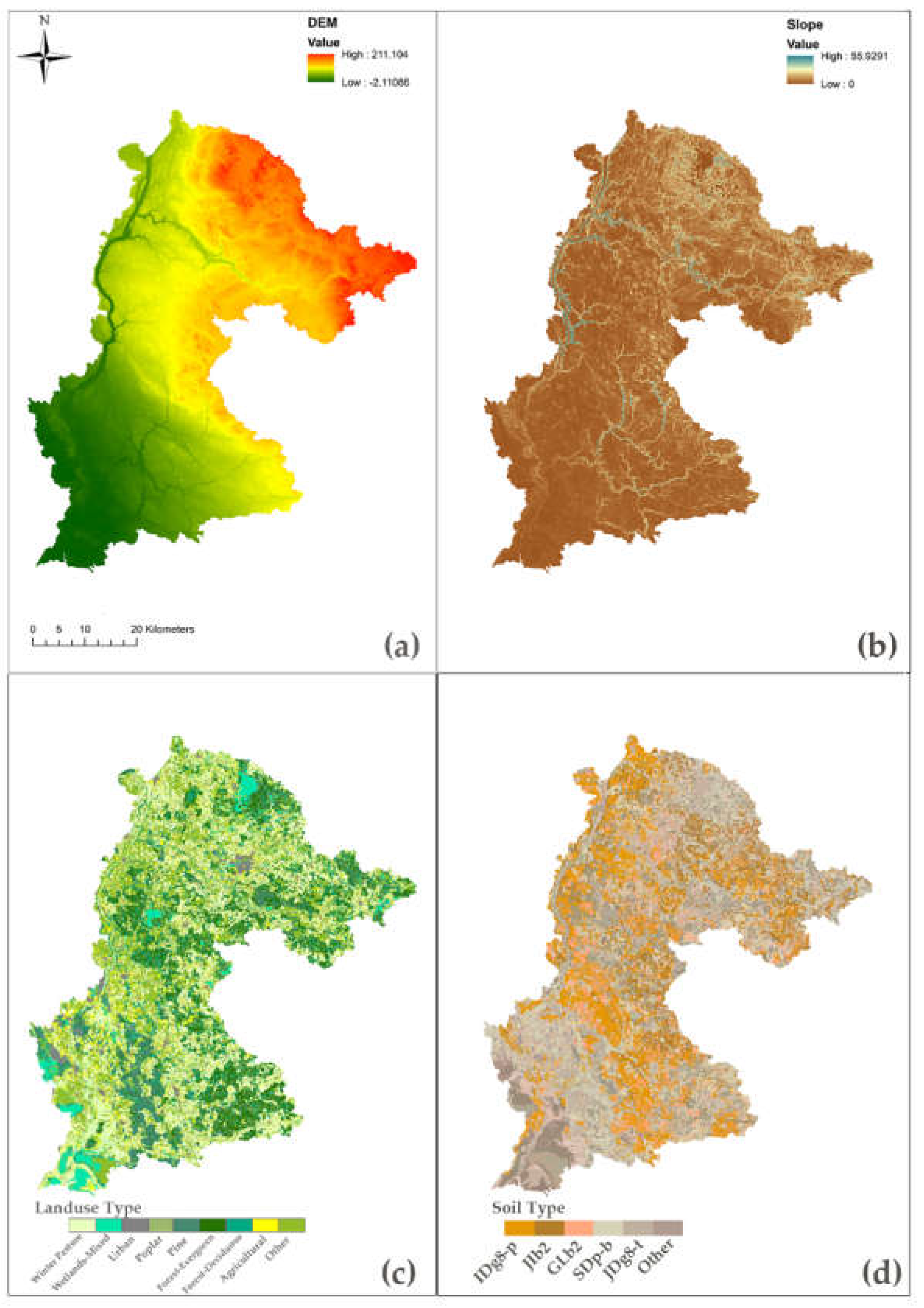
2.4. Data and Scenarios

Most of the data for this study region were attained from national databases of Lithuanian. The digital elevation model (DEM) and soil maps were attained from the National Land Service under the Ministry of Agriculture of Lithuania [44,45]. The original DEM resolution was 5 m × 5 m. Many studies discussed the optimum digital elevation model resolution for hydrological modelling, where most of them supported the statement “the spatially higher resolution the better”. Studies conducted by Ghaffari et al. (2011) and Goulden et al. (2014) [46,47] imply that higher resolution DEM produces more realistic results, whereas Cotter et al. (2003), Chaubey (2005) and Chang and Chao (2014) [48,49,50] focus on the decrease of uncertainty if higher resolution DEMs are utilized.
The DEM resolution was resampled to 35 m × 35 m. The topographical data was compiled from different sources covering all the Nemunas River drainage basin area, approximately to 100,000 km2, and extending to four countries: Lithuania, Belarus, Russia, and Poland. The model developed in this study is designed to be compatible with other watershed models within the Nemunas River Basin, where Minija Basin is a subwatershed. [29] suggested that an optimum spatial DEM resolution, where use of DEMs with very high resolution such as 1 m × 1 m or 3 m × 3 m are discouraged and 10 m × 10 m DEM spatial resolution, which are still of much higher resolution than the DEM used in this study, are suggested as optimum for hydrological modelling. Considering all the facts, we used a 35 m × 35 m DEM for topography which is the highest resolution that can be achieved in this study and can still be considered as spatially “not too high-resolution DEM” which is unsuggestable for general hydrological modelling. The land use dataset was created by combining the forest map from the State Forest Survey service under the Ministry of Environment of Lithuania, the Land Parcel Identification Database of Agri-information and rural business centre, and the spatial data set of georeferenced base cadastre from the Ministry of Agriculture of the Republic of Lithuania [51,52] data at a map scale of 1:10,000.
The characteristics of the waterbodies in the region were attained from the spatial data set of (geo) reference base cadastre of Lithuania [52]. The reported statistical crop yield data (used for soft calibration of the annual yields), livestock numbers (used for diffused pollution), population, and industries (used for point source discharge) were attained form the Statistical Yearbook of Lithuania [18].
The recorded weather conditions as well as observed flow and water quality data were attained from the Lithuanian Hydrometeorological Service under the Ministry of Environment. The records of flow, total nitrogen (TN), total phosphorus (TP), and sediment concentration were used to calibrate and validate the model. These records were available from the years 1995 to 2010 and were scattered over the watershed (Figure 4), meaning that different periods were available for different indicators from various locations in the basin; thus, a multi-site calibration was performed. Some of these gauging stations were constantly in use for performing daily monitoring of the river runoff, while others were in use for a short period. Minija–Lankupiai and Minija–Kartena are the runoff stations, which we used to calibrate flow on a monthly and daily basis (Figure 4). These are the only two stations with daily data available. Other stations (Minija near Suvernai, below Priekulė, below Gargždai, above and below Plongė) provided data mainly for nutrients (TN, TP) and sediment concentrations. The measurements in these stations have been taken, at best, twice per month, so there is a great deal of uncertainty attributed to them. Having no alternative, the water quality parameters were calibrated using monthly averages (in some cases represented by a single measurement) of these stations. We used the NS (Nash–Sutcliffe model efficiency coefficient), the R2 (coefficient of determination) and PBIAS (percent bias) to evaluate the model performance, as well as visual analysis of the hydrographs. A five-year warm-up period (from 1995–1999) was used to initiate the model.
Data for the climate change scenarios was prepared using the Climate Change Toolkit [53]. The projected changes for the 2020–2050 and 2051–2099 periods for temperature and precipitation from the HadGEM2-ES model, RCP 4.5 and 8.5 scenarios were used to assess the possible changes on the hydrologic regime and water quality of Minija River and the affected Lithuanian coastal zone region. The earth system components of HadGEM2-ES compare well with observations and with other models. In addition, stratospheric processes and variability are represented realistically [15]. HadGEM2-ES compares well with the C4MIP ensemble of models and was previously used in various assessments conducted in the Baltic region [12,14], therefore, we used the same model for comparative reasons. The humidity, wind speed and solar radiation data was generated by the SWAT weather generator [54], based on the average projected statistical values. The choice to analyse two different time horizons was dictated by the need on one side to work with a strong signal (long-term) and on the other side to investigate a period (near-term) that is not too far ahead for a future socio-economic analysis of the predicted changes. The scenario summary is presented in Table 1 and Table 2.
The changes in temperature projections display an overall increase in mean temperature in all seasons, most in summer months. Noteworthy is the fact that the projected changes in temperature for near-term are very similar for both RCPs (2a and 3a scenarios). Compared to the total set of representative concentration pathways, the RCP8.5 corresponds to the pathway with the highest greenhouse gas emissions, thus by the end of the century, the projections diverge [15] and the highest and most drastic changes are projected in this scenario by the end of 2100. The projected precipitation patterns show a net decrease of annual precipitation, although the distribution within seasons varies. All scenarios point to the increase of precipitation in spring months, while other seasons will receive less precipitation.
Minija River basin, as the majority of the territory of Lithuania, is a rain-fed watershed, meaning that there are no irrigation systems in place. The heat supply for the vegetation period will increase, and in summer, due to high temperatures and lack of moisture, the aridity of the territory will increase as well. This should serve as an early warning to the farmers of the region, due to a possible increase of hydrological draught frequency, which has already negatively affected the agriculture of Europe in recent years [55].

3. Results

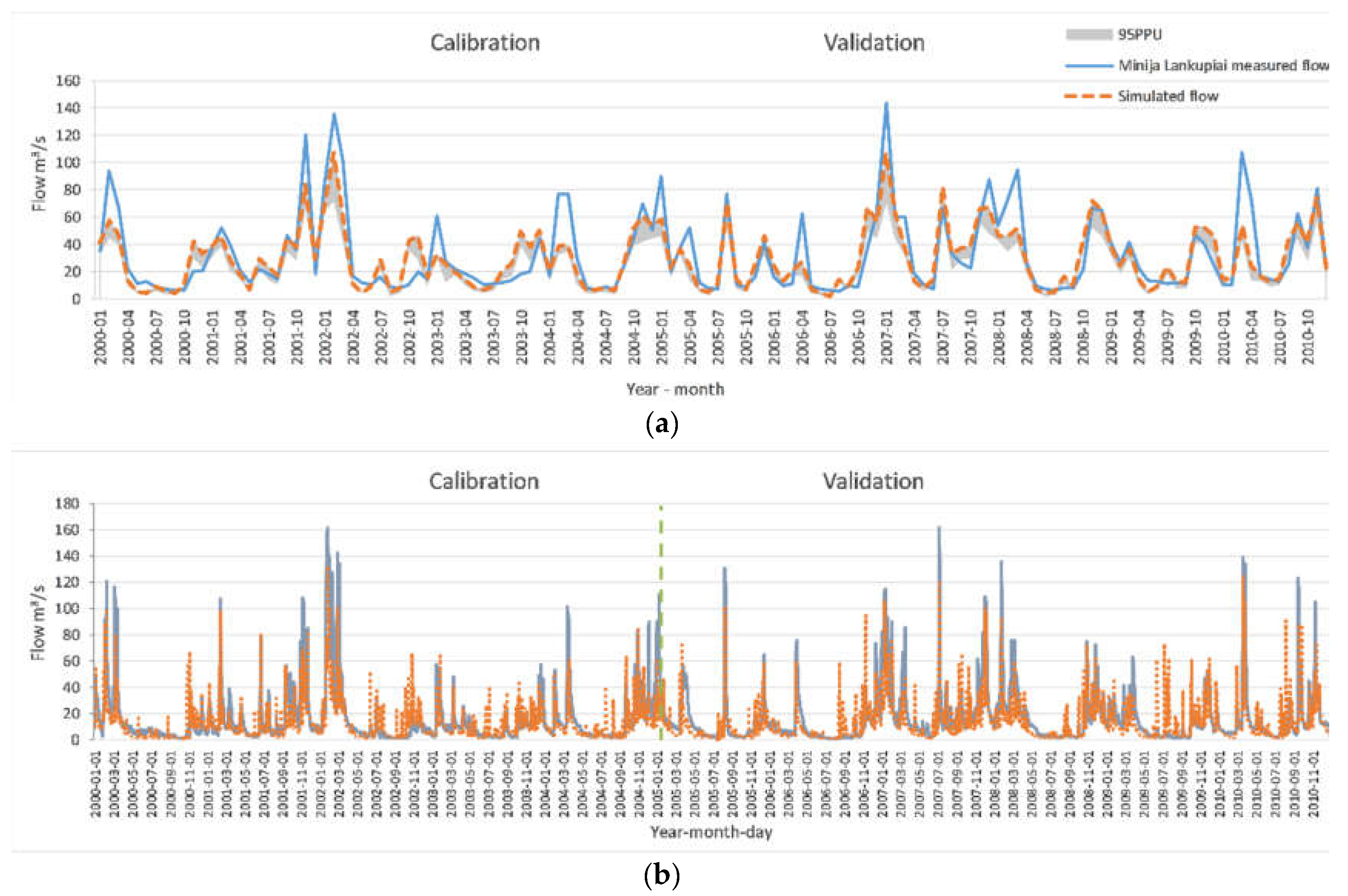
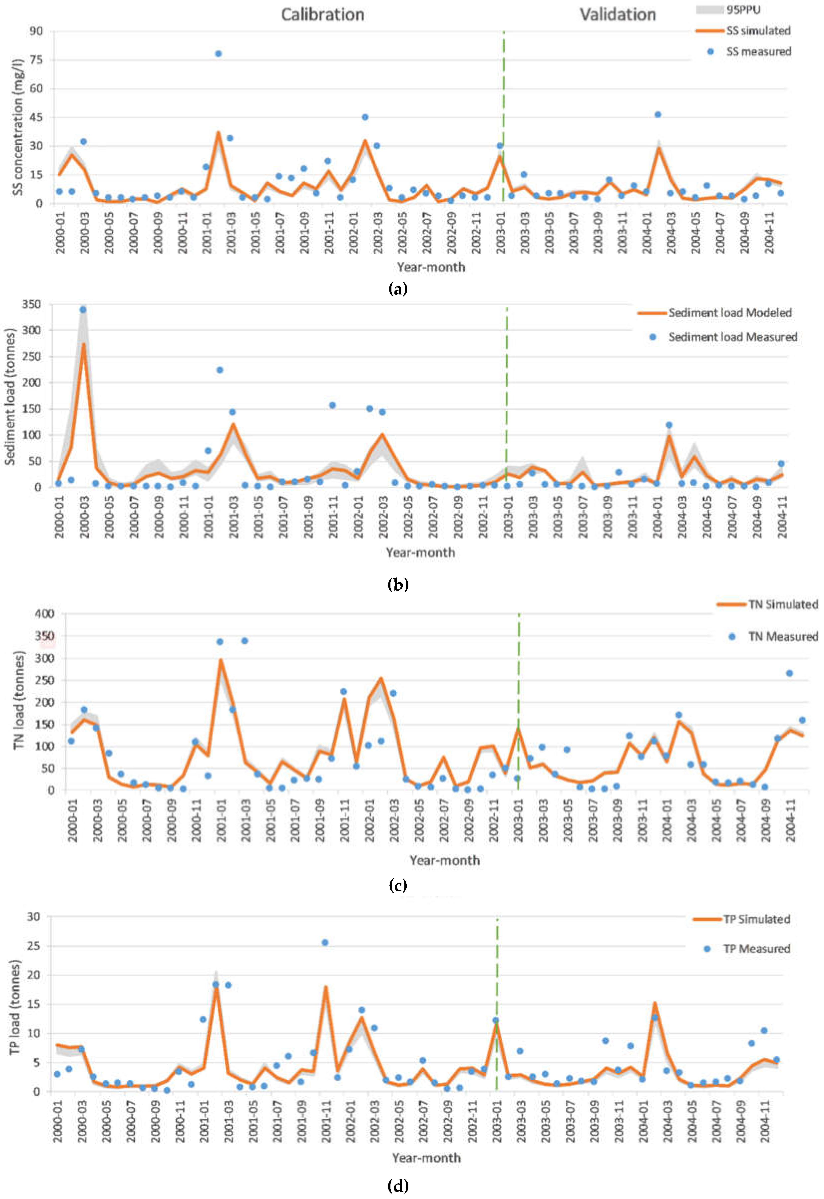
3.1. Model Calibration and Validation

A manual approach was used to calibrate and validate the model. Due to the comparatively long model runtime, we estimated that the automatic calibration procedure could last from 20 days (assuming the optimal parameter set would be determined in a single calibration iteration with 500 simulations), to up to three months. Being constrained by the time period to complete the study and the lack of computational resources, we decided to build upon previous calibrations of the Minija watershed [4] and our knowledge of the physical processes in the area. We recognize that the automatic calibration tools may provide a better solution for model parametrization and are considering quantifying this in the future.
The calibration procedure followed the general recommendations for SWAT model calibration [56], where one starts with flow calibration (baseflow plus surface runoff), then sediment and, finally, nutrients. Most of the model parameters were transferred from the previous study of SWAT model application (conducted with the SWAT 2009 version) for the Minija watershed [4]. In the ongoing study we are using the most recent available SWAT version 2018 (rev. 670) and are including the land management into the model, hence, a recalibration was essential. The parameters and their fitted values are presented in Table 3.
One systematic error of the model was the inability to simulate peak flows (Figure 5). This appears to be a common issue in a number of studies [57,58,59] and is a source of uncertainty that has to be taken into account. The high resolutions of DEM are reported to systematically underestimate runoff, due to the misestimation of runoff pathways and the overestimation of runoff contributing areas [43], hence, the water quality estimations in small streams, where the average flow was less than 3 m3/s, was affected in a negative way. This is an expected outcome because this particular variation of the Minija River model is setup to assess watershed-scale processes, thus, in some cases the small-scale information has been generalized by our simplification procedure. Furthermore, in the initial discretization, the threshold accumulation area for creating streams and reaches was set to 35 ha, thus every stream which has a drainage area attributed to it smaller than 35 ha was neglected.
Despite these drawbacks, we were able to calibrate and validate the model, providing an overall satisfactory performance statistic, according to Moriasi [60] (statistics are given in Table 4).
The calibration and validation for hydrology was performed on a monthly basis and, where available, on a daily one, and displayed an overall reasonable performance, with four stations delivering very good to satisfactory statistical performance (see example hydrographs in Figure 5) and three (Minija—above Plungė and below Plungė, Minija—near Suvernai) delivering non-satisfactory evaluation for R2. However, they were satisfactory for NS and PBIAS, according to the evaluation criteria for recommended statistical performance measures for watershed-scale models [60] (refer to Table 4). Stations around Plungė are situated in the upper part of the watershed, where the average streamflow is approx. 5 m3/s. Furthermore, the measurements in these particular stations were taken usually once per month with a varying interval. In some cases, a 20-day interval resulted in a six-fold increase in flow. Apparently, this data series is best used for annual calibration, rather than monthly, as a single observation cannot be representative for the entire period.
To calibrate the sediment yield we first analysed and statistically evaluated the performance of each sediment routing method, and selected the one which displayed a better fit with the observations—the Simplified Bagnold Equation method. After this, we manually adjusted the parameters related to sediment load to the stream and channel erodibility factor to achieve the best fit with measured data (see Table 3). The only available measurement for sediments was the suspended sediment concentration at station Minija—below Gargždai. Here, we have encountered a similar issue, as in our previous study (see Čerkasova et al. [14] for more details), where there was a lot of uncertainty attributed with the measurements, i.e., we did not know the mesh size used to take samples, what was the exact location of the sampling, etc. Having no alternative, we used these data for calibration and validation, achieving satisfactory performance for sediment load (R2 = 0.6 for calibration and R2 = 0.56 for validation, NS = 0.54 for calibration and NS = 0.53 for validation) (see Figure 6 top and second graphs).
The calibration and validation for TN produced an overall good to satisfactory results (see he example in Figure 6c). The situation with nutrient calibration performance statistics values were similar to those for flow calibration. One must keep in mind that the primary source of low performance for nutrient load calibration comes from poor representation of hydrologic conditions for that particular station. But that does not mean that the model fails to represent the overall (net effect) picture of the processes, especially judging by the fact that our model produces good (in some cases very good) model fit for flow, TN, and TP for stations, which are in the lower parts of the watershed.
The performance for TP ranged from very good (in Minija—below Gargždai) to satisfactory (Minija—near Suvernai) (Table 4). Usually, the calibration and validation results for phosphorus is similar to those of sediments, as the particulate form is the one that is usually being transported in the watershed. Sicne the only point, which was calibrated for sediments, was in the sub-basin of “Minija—below Gargždai” station, it is expected that the model will perform good for phosphorus in that location as well (see Figure 6d). As it became apparent in our previous study [14], the input of P to streamflow from groundwater is an issue in the Nemunas River watershed, at least in the upper sub-basins. A similar characteristic might be applicable for the Minija River basin as well. However we did not find any reliable sources, which could provide us with the precise concentration of phosphorus (usually PO4) in the groundwater, while the Lithuanian Environmental Protection Agency [61] suggests that the water quality of Lithuanian groundwater is poor. We used the values for soluble P contribution that provided the best model fit in the calibration period (see Table 3), which is on par with general groundwater PO4 concentration values declared in the reports from the Lithuanian Environmental Protection Agency [62].
To sum up, we deemed the model suitable for predicting the average annual and seasonal discharge, TN, and TP load of the Minija River basin and proceeded with scenario evaluation.

3.2. Predicted Average Yearly Changes in the Minija Basin

Some general changes of the entire basin are summed up and presented in the Table 5. On average by the end of the century, the amount of precipitation received by the area will decrease (from 776.6 mm to 661 mm in RCP 4.5, and 668 under RCP 8.5). A drastic decrease, by approx. 60%, in the snowfall is predicted, hence confirming the multiple studies that indicate an overall decrease in snow cover in the northern parts of Europe [62].
One interesting result that requires some explanation is the total nitrogen and total phosphorus loading. In both RCPs, the amount of nutrient loads decreases. This is associated with different factors for T and P. The amount of nitrogen transported with water (the concentration of constituents attributed to N) will not change by much in RCP 4.5, although, according to the model output for the RCP 8.5, it is expected to increase by 2%, which is a minor change. So, the decrease of TN load is attributed mainly to the change in flow, which is projected to decrease by 35% (from 38 m3/s to 24.6 m3/s) in RCP 4.5, and by 30% (to 26.4 m3/s) in RCP 8.5 (Table 5).
The modelled amount of phosphorus (concentration of constituents attributed with P) transported with waters of Minija River to the mouth will decrease by 30% in RCP 4.5, and by 11% in RCP 8.5. This is a similar finding as the one made in another part of the Nemunas River sub-basin—the Vilija River sub-basin (for more detail see Čerkasova et al. (2018) [14]). Although it is difficult to identify the reason behind the overall decrease of the P load, we assume it is associated with the point source contributions and with groundwater. We used the average point source contributions for the past five years in our study, which has changed dramatically, compared to the early years of the baseline scenario, due to renewal of sewage treatment plants in the area.
Phosphorus loading may contribute to the streamflow from different sources. It was determined by our pervious study [14] that there is phosphorus loading from the groundwater to the streamflow of the Nemunas River watershed. Minija River, as a part of the Nemunas watershed, also experiences significant groundwater contribution to the streamflow. Considering this point, we analysed the change in the constituents of the streamflow under the climate change forcing; thus, the change in the net phosphorus load became apparent: the groundwater contribution to the streamflow is modelled to decrease by 35% under conditions of the RCP 4.5, and by 28% under RCP 8.5. This is the reason why the modelled phosphorus load is projected to decrease under the changing climate conditions.
The decadal analysis of precipitation and ET variability (see Figure 7) sheds some light onto the changes in these and related processes. The total average ET is projected to gradually increase during winter months: from 3.5 mm in the baseline to 16.76 mm in RCP 4.5 and 22.21 mm in RCP 8.5); and during spring: from 79.84 mm in the baseline to 129.14 mm and 132.81 mm in RCP 4.5 and 8.5 respectively. The changes in ET in the summer months vary from decade to decade, and in fall the ET does not change much over the century. However, precipitation patterns display a somewhat different trend.
The total average precipitation during winter months decrease gradually through the decades, never reaching the values of the baseline period (178.31 mm), while in spring there is an increase in rainfall, received by the basin: from 115.97 mm in the baseline to 173.07 mm and 177.86 mm by the end of the century in RCP 4.5 and 8.5, respectively. The largest net decrease in precipitation is simulated in the summer months for the RCP 8.5: from 257.24 mm to 159.66 mm; and in fall for RCP 4.5, from 234.29 mm to 150.91 mm. Still, both summer and fall periods are projected to receive on average much less precipitation: 30.7% and 23.1% for summer and fall in RCP 4.5; and 32.42% and 22.6% in RCP 8.5, meaning that the area will become more arid in this time of the year.

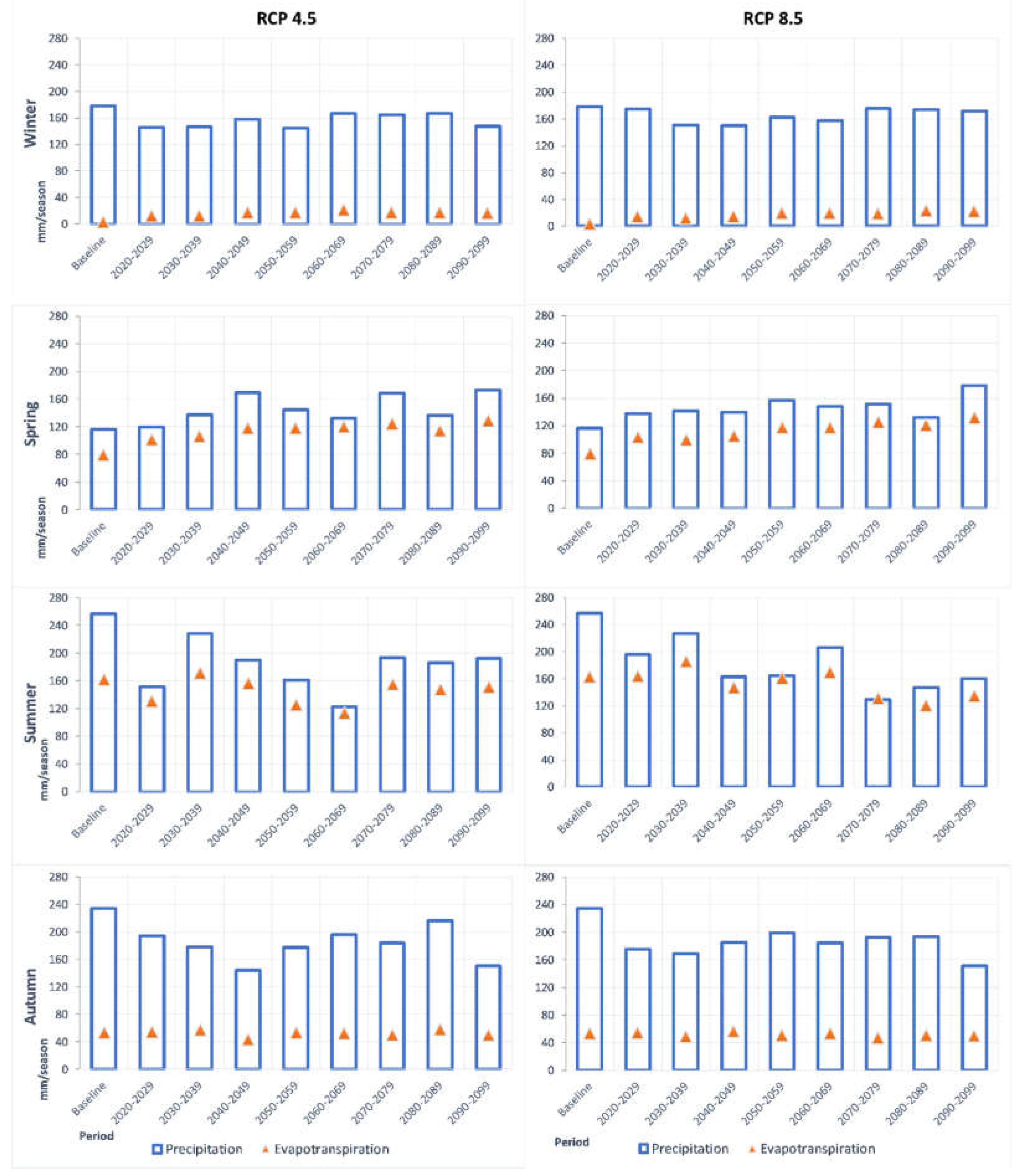
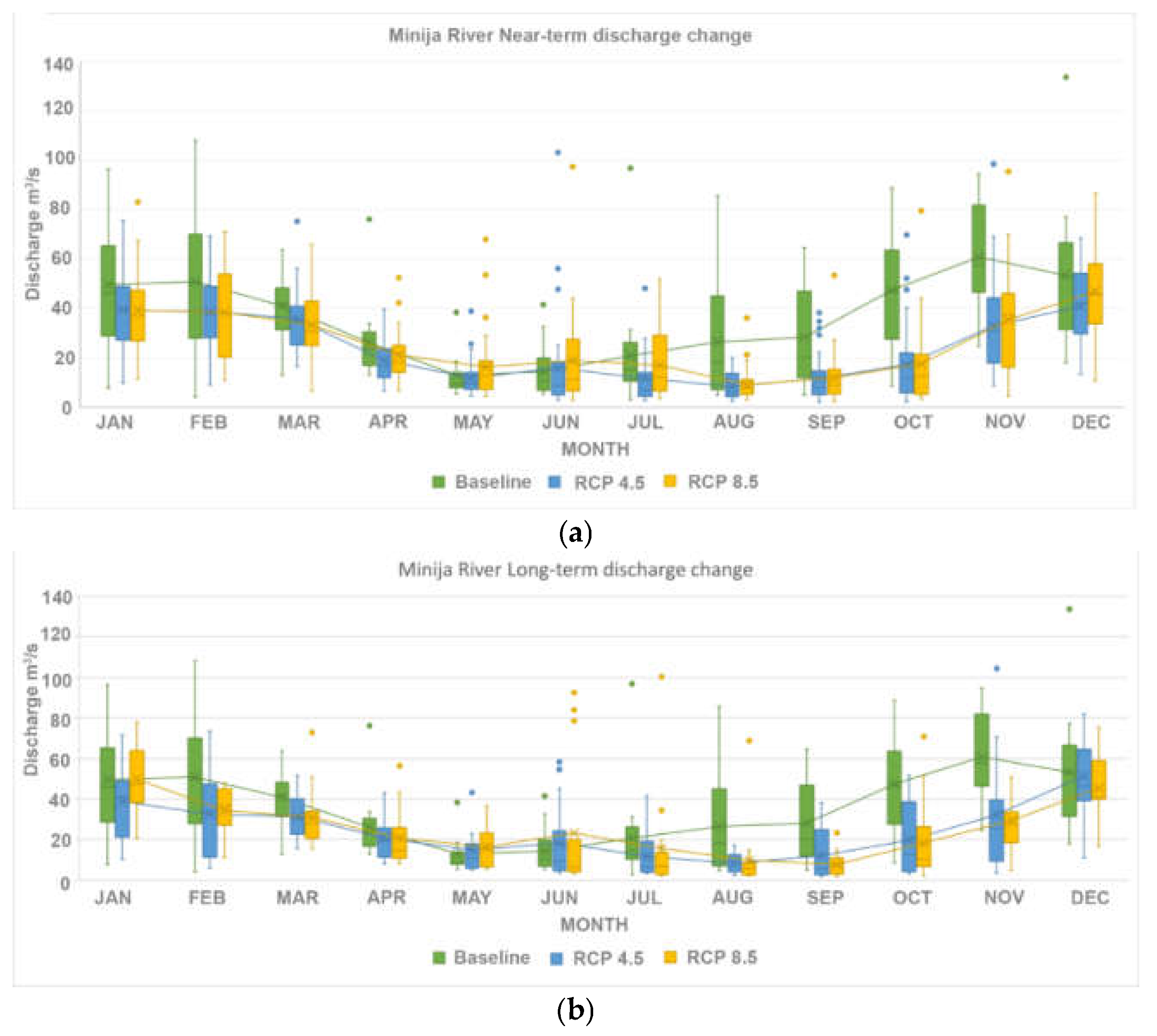
3.3. Predicted Changes in the Hydrological Regime

3.3.1. Minija River Near-Term Flow Changes

Apart from the projected annual and decadal changes in the watershed, we analysed the inter-seasonal changes in the flow regime of the river for both near- and long-term periods. Following the projected changes in precipitation, it is apparent that for most months the flow will decrease. This can be clearly seen in the period from August to November (Figure 8), while differences among other months are not substantial, i.e., May.
The minimum monthly flow rates are projected to experience a change mostly during October–November months, whereas the maximal monthly flow will change substantially in the period from July–November.
Apart from maximum, minimum, average, and median flow changes, there is a substantial amount of outliers present in the simulations of both RCPs, although their number differs from month to month. The outliers a present only for high flows, resulting from storm (or severe precipitation) events, which are considered to increase in frequency and in intensity in the future climate predictions [62].
The most notable difference between the two scenarios can be observed in May, when in RCP 4.5 a decrease in the mean flow is projected, where under the RCP 8.5 an increase is modelled, although the statistics might be biased due to outliers modelled for this month under RCP 8.5. A substantial difference in the mean discharge and flow distribution is also projected in June and July, with some outliers present as well.

3.3.2. Minija River Long-Term Flow Changes

In January, RCP 8.5 simulates streamflow conditions close to those of the baseline, where RCP 4.5 indicates a significant decrease in the streamflow. February, March, and April will experience a decrease in streamflow as well, although May and June indicate a possibly slight increase in average flow, and an increase in the number of outliers. The agreement between streamflow outputs under both RCPs from July to December is high, indicating similar model responses to climate change forcing. A decrease in flow, compared to the baseline, is projected under each scenario, with a more significant decrease from September to December under RCP 8.5. The outliers occur, but not as frequent as in the near-term period.

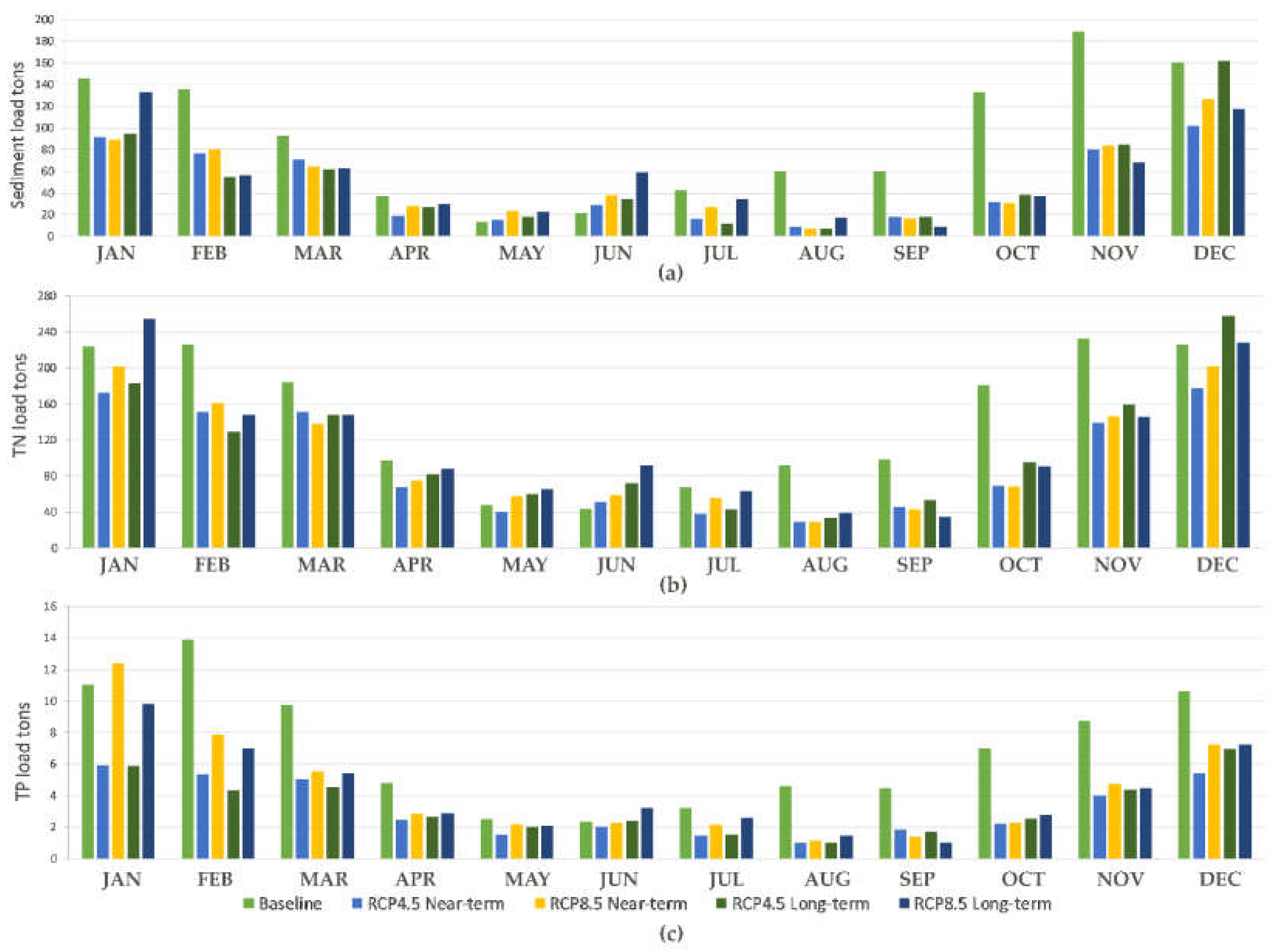
3.4. Predicted Average Monthly Sediment and Nutrient Loads

3.4.1. Minija River Near-Term Sediment and Nutrient Loads

The total average sediment loads decrease through the near-term period by 48.8% in RCP 4.5 and by 43.6% in RCP 8.5. May and June are the only months which are projected to yield more sediment loadings in the near future for both RCPs, with a more prominent change in the RCP 8.5 (Figure 9a). Other months experience a significant reduction of sediment loading. This is mirrored in the projected hydrological changes (Figure 8a), where the average runoff during these particular months increase compared to the baseline.
As already mentioned, the decrease in nutrient loads is a consequence of both, the total water yield and composition of streamflow. For nitrogen, being a highly mobile element, the total discharge will have the most influence on the loads, whereas the sources of phosphorus load to the streamflow is the main governing process in the TP load.
The projected changes in the average loads of nitrogen display a similar trend under the conditions of PRC 4.5 and 8.5 (see Figure 9b), where a general decrease for each month (except variations in May and June) is modelled. The most significant decrease is expected from August to November, the same period as the most changes in flow rates. The period from April to July will experience less change, with an insignificant increase modelled in RCP 8.5, compared to RCP 4.5.
The changes in phosphorus loads followed the same tendency of decrease, although with some variations from month to month (see Figure 9c). A significant change is found in the projected TP load, where a significant reduction is modelled under the conditions of RCP 4.5; but an increase in TP load is expected under RCP 8.5. On average, the projected decrease in TP load is more significant in RCP 4.5, compared to RCP 8.5.

3.4.2. Minija River Long-Term Nutrient and Sediment Loads

The long-term period indicates similar changes, as in the near-term, meaning that there are no significant changes in the system during the second half of the century, although some differences can be found. A yearly net decrease is projected for sediment loads: by 43.9% in RCP 4.5 and by 40.9% in RCP 8.5. As in the near-term, the long-term changes for May and June indicate an increase in sediment loading (Figure 9a), with a very prominent increase in June in RCP 8.5 (by 180% compared to the baseline). The sediment loadings for January and December mirror the differences in the projected hydrological changes for the long-term situation between the two RCPs (see Figure 8b) in these particular months. In January, the average flow is projected to be more in RCP 8.5, and in December, RCP 4.5 conditions yield more streamflow. This results in the same patterns of projected sediment loads for the long-term period.
One noticeable change is in the total N load under RCP 8.5: it is projected to increase in January, May and June (Figure 9b). The projected changes in N loads in winter might be explained by the reduced snow cover in the region by the end of the century (See Table 5). As the Minija river basin is situated in a cold-climate region, where the vegetation during winter goes dormant, the nutrient wash-off will evidently increase. This hypothesis is also supported by the model results in the decrease of temperature stressed days summarized in Table 5. As for May and June—the streamflow projection for the RCP 8.5 indicates a slight increase during these months (Figure 8b). According to model results, the net amount of nutrients that are brought downstream from the basin are expected to change similarly to the streamflow. This might be a concern for the possible blooms in the Curonian lagoon, although currently the Minija River is a small contributor, compared to the Nemunas River, which brings the majority of nutrients to the lagoon.
The TN increase is also projected in December, May, and June under RCP 4.5. We suggest that the explanation for this is the same, as in the case of RCP 8.5: the projected streamflow increase will result in a net increase of nutrient load.
The TP load is projected to increase only in June under RCP 8.5 (Figure 9c), while a decrease in total load is projected in the rest of the months for both RCPs in the long-term period. This could potentially be a problem for the Curonian lagoon, as phosphorus becomes a limiting nutrient during warm periods [63].

4. Discussion

4.1. Possible Changes Related to Hydrologic Regime Change

This study of the Minija River basin is a contribution to the fine-grid large-scale model development, where the ultimate goal is to assess the entire Nemunas River watershed in terms of hydrology, nutrient, and sediment loads under a changing climate.
We determined that there are significant differences within the Nemunas watershed in the response to various forcing factors. Where the hydrological response from Vilija River basin (the east-most sub-basin of the Nemunas River watershed; see Figure 1) under the conditions of RCP 4.5 and RCP 8.5 showed an increase in flow for all months, the projected changes in the Minija River basin (west-most sub-basin on the Nemunas River watershed) are quite the opposite (Figure 8) [14]. Basing our assumptions on the differences between these areas, we expect to see different responses of various sub-basins of the Nemunas watershed to projected climate change, when the final modelling framework will be completed.
Based on the average annual output of the model (Table 5), both under RCP 4.5 and RCP 8.5 near-term and long-term, it is probable that the coastal area of Lithuania will receive less precipitation (on average 14% less) of which snow fall will decrease substantially (by 60%), but will experience drier and warmer days, increasing the vegetation period in the area. As a result, this will have a significant impact on the average yearly Minija River discharge and the streamflow composition. A significant number of outliers in the warmer months (April to July) in both RCPs for long and short-term periods indicate the possible contribution of storm events, which are projected to be more frequent in the future [62]. The warmer climate also points to the more frequent occurrence of droughts, which can cause significant economic damage. As an interesting finding, we can conclude that a yearly net effect on the watershed is more significant in RCP 4.5, rather than in the conditions of RCP 8.5 which is usually associated with a more prominent change in the global weather patterns.

4.2. Possible Changes Related to Nutrient Loads

The changes in the nutrient loads follow a similar trend of decrease in a similar manner as the total discharge of the river, although the relationship is not linear. The changes in TN load is mainly attributed to the change in flow rates, as the concentration of N will not be affected significantly by changes in climate. While performing the scenario simulations for both RCPs, we assumed that the land cover, land management and the point source contributions would not change for the entire period (long and short-term). Of course, we recognize that these changes will occur in the watershed, alongside some socio-economic and political changes, but at this point, our intention was to explore the influence of only the climate forcing. We can conclude that with no change in the land management, the land-based nitrogen load will not decrease; only the transported amount (the net mass) will change.
The results in the projected TP load change display a different pattern, although they still show a decreasing trend for both short-term and long-term periods in both RCPs. It seems that the TP change is highly influenced by the groundwater contribution to the streamflow. Since the streamflow composition of the Minija River will change, so will the amount of phosphorus transported with the stream. Although studies suggest that the influence of anthropogenic factors on phosphorus loads, such as point source loads from sewage treatment plants, are the major ones [64], we found that the groundwater constituent and the phosphorus concentration in it are equally important in the Minija River basin and will remain as such in the future, if no significant changes in the anthropogenic activities will occur.
One alarming outcome is the increase in phosphorus and sediment loads in the months of May and June. In the warmer season, the hypereutrophic Curonian Lagoon experiences algal blooms, especially in the southern part. Phosphorus load increase in this season might enhance the frequency and intensity of the blooms. However, the inputs of nutrients to the lagoon from the Minija River are not large compared to the Nemunas River, thus, these changes might by negligible for a large system. A more detailed study is needed to quantify the effect of each contributor of nutrients to the lagoon and assess the possibilities and threats associated with the future changes of the loads. If the rest of the Nemunas River watershed will follow a similar trend, then we can assume a net reduction of nutrient and sediment loads to the Curonian Lagoon and hence, to the Baltic Sea, will occur in the future, as projected by the RCP 4.5 and RCP 8.5 scenarios. We are currently working on the rest of the modelling framework for the remaining parts of the Nemunas River watershed and we intend to test this hypothesis.
Since there are dissimilarities in the hydrological and nutrient load response throughout the Nemunas River watershed to climate forcing, we suggest that a unified strategy for adaptation to climate change, planning and implementation of measures to reduce nutrient inputs in the Baltic Sea region might not be the optimal solution. The nutrient load assessments for determining the Maximum Allowable Levels could incorporate a similar strategy as in this study, where a large area (i.e., country) is divided into sub-regions and assessed separately within a net effect of the area, thus creating a more targeted (hot-spot) analysis of major polluters. Furthermore, this study indicates that the nutrient load from coastal areas of the East Baltic might reduce under the conditions of climate change, although anthropogenic activity might reverse this effect.

4.3. Future Work

Our future work includes the combination of all the modelled areas of the Nemunas River watershed (see Figure 1) to produce a modelling framework that could assess the influence of climate change, to analyse the scenarios for future programmes of measures for improving the water quality (including best management practices using built-in modelling options in SWAT) in the entire watershed and in different sub-basins. The framework must be sufficiently detailed, as we plan to assess possible nutrient retention measures and their effectiveness on the entire region. For this, we will have to evaluate our proposed simplification procedure (see Supplementary Material B) on the model run time, accuracy and test it on multiple case studies, with guidelines on the effectiveness of such simplifications and tradeoffs to follow.
The model of the Minija River watershed will be used further in the context of the EcoServe project to conduct an ecosystem services assessment in the region, as well as a tool to guide the local policymakers on regional development strategy planning. We intend to run multiple land use and socio-economic change scenarios, which will enable us to detect the changes in the related ecosystem services in the region as well as identify possible emerging ecosystem services. Furthermore, the watershed model will be coupled with the Curonian Lagoon hydrodynamic model (SHYFEM) [65,66] to assess the ecosystem services related to water availability and water quality of the coastal areas of Lithuania.
Our findings indicate that there is a gap in the knowledge of the streamflow composition of the rivers in the Nemunas watershed. A study that analyses the current and past streamflow composition would be a good contribution to understanding the consequences and the changes in the nutrient loads to the Curonian Lagoon. Along with other studies, this is something that we plan to investigate in the future.

Supplementary Materials

The following are available online at https://www.mdpi.com/2073-4441/11/4/676/s1, Supplementary Material A: Soil and Water Assessment Tool (SWAT) model description, Supplementary Material B: Methodology for Hillslope delineation and data simplification, Supplementary Material C: CN values for different landuses.

Author Contributions

Conceptualization: N.Č., A.E., and G.U.; methodology: N.Č. and A.E.; software: N.Č. and A.E.; validation: N.Č.; formal analysis: N.Č.; investigation: N.Č and A.E.; data curation: N.Č.; writing—original draft preparation: N.Č.; writing—review and editing: N.Č., A.E., and G.U.; visualization: N.Č.; supervision: G.U.; funding acquisition: G.U.

Funding

This research is funded by the European Social Fund according to the activity ‘Improvement of researchers’ qualification by implementing world-class R and D projects’ of Measure No. 09.3.3-LMT-K-712.

Acknowledgments

The carried-out modelling study is a part of the EcoServe project “The future ecosystem services of the Lithuanian coastal zone: the global change perspective”. We would like to thank EcoServe project team members Petras Zemlys and Jovita Mėžinė for their input.

Conflicts of Interest

The authors declare no conflict of interest.

References

  1. HELCOM. Thematic Assessment of Eutrophication 2011–2016; HELCOM: Helsinki, Finland, 2018; Available online: http://www.helcom.fi/baltic-sea-trends/holistic-assessments/state-of-the-baltic-sea-2018/reports-and-materials (accessed on 7 January 2019).
  2. HELCOM Ministerial Meeting. In HELCOM Baltic Sea Action Plan; HELCOM: Krakow, Finland, 2007.
  3. Svendsen, L.M.; Larsen, S.E.; Gustafsson, B.; Sonesten, L.; Frank-Kamenetsky, D. Progress Towards National Targets for Input of Nutrients; HELCOM: Helsinki, Finland, 2018. [Google Scholar]
  4. Čerkasova, N.; Ertürk, A.; Zemlys, P.; Denisov, V.; Umgiesser, G. Curonian Lagoon drainage basin modelling and assessment of climate change impact. Oceanologia 2016, 58, 90–102. [Google Scholar] [CrossRef]
  5. Graham, L.P. Climate Change Effects on River Flow to the Baltic Sea. AMBIO J. Hum. Environ. 2004, 33, 235–241. [Google Scholar] [CrossRef]
  6. Donnelly, C.; Yang, W.; Dahné, J. River discharge to the Baltic Sea in a future climate. Clim. Chang. 2014, 122, 157–170. [Google Scholar] [CrossRef]
  7. c/o International Baltic Earth Secretariat. Second Assessment of Climate Change for the Baltic Sea Basin; Bolle, H.-J., Menenti, M., Rasool, S.I., Eds.; Springer International Publishing AG Switzerland: Cham, Switzerland, 2015; ISBN 978-3-319-16005-4. [Google Scholar] [CrossRef]
  8. Rimkus, E.; Kažys, J.; Bukantis, A.; Krotovas, A. Temporal variation of extreme precipitation events in Lithuania. Oceanologia 2011, 53, 259–277. [Google Scholar] [CrossRef]
  9. Stonevičius, E.; Rimkus, E.; Štaras, A.; Kažys, J.; Valiuškevičius, G. Climate change impact on the nemunas river basin hydrology in the 21st century. Boreal Environ. Res. 2017, 22, 49–65. [Google Scholar]
  10. Cousino, L.K.; Becker, R.H.; Zmijewski, K.A. Modeling the effects of climate change on water, sediment, and nutrient yields from the Maumee River watershed. J. Hydrol. Reg. Stud. 2015, 4, 762–775. [Google Scholar] [CrossRef]
  11. HELCOM. BASE project 2012–2014. In Assessment and Quantification of Nutrient Loads to the Baltic Sea from Kaliningrad Oblast and Transboundary Rivers, and the Evaluation of their Sources; Baltic Marine Environment Protection Commission HELCOM: Helsinki, Finland, 2014; Available online: http://www.helcom.fi/Lists/Publications/Nutrient%20monitoring%20in%20Kaliningrad_BASE%20Project%20Final%20Report.pdf (accessed on 5 December 2018).
  12. Povilaitis, A.; Widén-Nilsson, E.; Šarauskienė, D.; Kriaučiūnienė, J.; Jakimavičius, D.; Bukantis, A.; Kažys, J.; Ložys, L.; Kesminas, V.; Virbickas, T.; et al. Potential impact of climate change on nutrient loads in lithuanian rivers. Environ. Eng. Manag. J. (EEMJ) 2018, 17, 2229–2240. [Google Scholar] [CrossRef]
  13. Meier, H.E.M.; Hordoir, R.; Andersson, H.C.; Dieterich, C.; Eilola, K.; Gustafsson, B.G.; Höglund, A.; Schimanke, S. Modeling the combined impact of changing climate and changing nutrient loads on the Baltic Sea environment in an ensemble of transient simulations for 1961–2099. Clim. Dyn. 2012, 39, 2421–2441. [Google Scholar] [CrossRef]
  14. Čerkasova, N.; Umgiesser, G.; Ertürk, A. Development of a hydrology and water quality model for a large transboundary river watershed to investigate the impacts of climate change—A SWAT application. Ecol. Eng. 2018, 124, 99–115. [Google Scholar] [CrossRef]
  15. Martin, G.M.; Bellouin, N.; Collins, W.J.; Culverwell, I.D.; Halloran, P.R.; Hardiman, S.C.; Hinton, T.J.; Jones, C.D.; McDonald, R.E.; McLaren, A.J.; et al. The HadGEM2 family of Met Office Unified Model climate configurations. Geosci. Model Dev. 2011, 4, 723–757. [Google Scholar] [CrossRef]
  16. SWAT Literature Database for Peer-Reviewed Journal Articles. Available online: https://www.card.iastate.edu/swat_articles/ (accessed on 18 June 2018).
  17. Arnold, J.G.; Kiniry, J.R.; Srinivasan, R.; Williams, J.R.; Haney, E.B.; Neitsch, S.L. Soil and Water Assessment Tool “SWAT” Input/Output Documentation; SWAT: Houston, TX, USA, 2012. [Google Scholar]
  18. Lietuvos Statistikos Departamentas/Statistics Lithuania. Lietuvos Statistikos Metraštis/Statistical Yearbook of Lithuania; The Lithuanian Department of Statistics: Vilnius, Lithuania, 2017.
  19. Umgiesser, G.; Čerkasova, N.; Erturk, A.; Mėžinė, J.; Kataržytė, M. New beach in a shallow estuarine lagoon: A model-based E. coli pollution risk assessment. J. Coast. Conserv. 2018, 22, 573–586. [Google Scholar] [CrossRef]
  20. Volungevičius, J.; Kavaliauskas, P. Lietuvos Dirvožemiai; Aleksandras Stulginskis University: Kaunas, Lithuania, 2012. [Google Scholar]
  21. Belda, M.; Holtanová, E.; Halenka, T.; Kalvová, J. Climate classification revisited: From Köppen to Trewartha. Clim. Res. 2014, 59, 1–13. [Google Scholar] [CrossRef]
  22. Arnold, J.G.; Allen, P.M.; Volk, M.; Williams, J.R.; Bosch, D.D. Assessment of Different Representations of Spatial Variability on SWAT Model Performance. Trans. ASABE 2010, 53, 1433–1443. [Google Scholar] [CrossRef]
  23. Hesse, C.; Krysanova, V.; Päzolt, J.; Hattermann, F.F. Eco-hydrological modelling in a highly regulated lowland catchment to find measures for improving water quality. Ecol. Model. 2008, 218, 135–148. [Google Scholar] [CrossRef]
  24. Kim, N.W.; Shin, A.H.; Lee, J. Effects of Streamflow Routing Schemes on Water Quality with SWAT. Trans. ASABE 2010, 53, 1457–1468. [Google Scholar] [CrossRef]
  25. Jencso, K.G.; McGlynn, B.L.; Gooseff, M.N.; Bencala, K.E.; Wondzell, M.S. Hillslope hydrologic connectivity controls riparian groundwater turnover: Implications of catchment structure for riparian buffering and stream water sources. Water Resour. Res. 2010, 46, 1–18. [Google Scholar] [CrossRef]
  26. Kraft, P.; Haas, E.; Klatt, S.; Kiese, R.; Butterbach-Bahl, K.; Frede, H.-G.; Breuer, L. Modelling nitrogen transport and turnover at the hillslope scale—A process oriented approach. In Proceedings of the 6th International Congress on Environmental Modelling and Software: Managing Resources of a Limited Planet, Leipzig, Germany, 1–5 July 2012. [Google Scholar]
  27. Vigiak, O.; Malagó, A.; Bouraoui, F.; Vanmaercke, M.; Poesen, J. Adapting SWAT hillslope erosion model to predict sediment concentrations and yields in large Basins. Sci. Total Environ. 2015, 538, 855–875. [Google Scholar] [CrossRef]
  28. Zhao, Y.; Beighley, E. Upscaling Surface Runoff Routing Processes in Large-Scale Hydrologic Models: Application to the Ohio River Basin. J. Hydrol. Eng. 2016, 22, 04016068. [Google Scholar] [CrossRef]
  29. Hoang, L.; Schneiderman, E.M.; Moore, K.E.B.; Mukundan, R.; Owens, E.M.; Steenhuis, T.S. Predicting saturation-excess runoff distribution with a lumped hillslope model: SWAT-HS. Hydrol. Process. 2017, 31, 2226–2243. [Google Scholar] [CrossRef]
  30. Vigiak, O.; Malagó, A.; Bouraoui, F.; Vanmaercke, M.; Obreja, F.; Poesen, J.; Habersack, H.; Fehér, J.; Grošelj, S. Modelling sediment fluxes in the Danube River Basin with SWAT. Sci. Total Environ. 2017, 599–600, 992–1012. [Google Scholar] [CrossRef]
  31. Gorgan, D.; Bacu, V.; Mihon, D.; Rodila, D.; Abbaspour, K.; Rouholahnejad, E. Grid based calibration of SWAT hydrological models. Nat. Hazards Earth Syst. Sci. 2012, 12, 2411–2423. [Google Scholar] [CrossRef]
  32. Pignotti, G.; Rathjens, H.; Cibin, R.; Chaubey, I.; Crawford, M. Comparative analysis of HRU and grid-based SWAT models. Water 2017, 9, 272. [Google Scholar] [CrossRef]
  33. Scanlon, B.R.; Keese, K.E.; Flint, A.L.; Flint, L.E.; Gaye, C.B.; Edmunds, W.M.; Simmers, I. Global synthesis of groundwater recharge in semiarid andaridregions Bridget. Hydrol. Process. 2006, 20, 3335–3370. [Google Scholar] [CrossRef]
  34. Qin, C.-Z.; Liu, J.-Z.; Zhu, A.-X.; Zhu, L.-J.; Gao, H.-R.; Wu, H. Spatial optimization of watershed best management practices based on slope position units. J. Soil Water Conserv. 2018, 73, 504–517. [Google Scholar] [CrossRef]
  35. Zhu, L.J.; Qin, C.Z.; Zhu, A.X.; Liu, J.; Wu, H. Effects of different spatial configuration units for the spatial optimization of watershed best management practice scenarios. Water 2019, 11, 262. [Google Scholar] [CrossRef]
  36. Bieger, K.; Arnold, J.G.; Rathjens, H.; White, M.J.; Bosch, D.D.; Allen, P.M.; Volk, M.; Srinivasan, R. Introduction to SWAT+, A Completely Restructured Version of the Soil and Water Assessment Tool. J. Am. Water Resour. Assoc. 2017, 53. [Google Scholar] [CrossRef]
  37. Linker, L.C.; Shenk, G.W.; Wang, P.; Hopkins, K.J.; Pokharel, S. A Short History of Chesapeake Bay Modeling and the Next Generation of Watershed and Estuarine Models. Proc. Water Environ. Fed. 2012, 2002, 569–582. [Google Scholar] [CrossRef]
  38. Shenk, G.W.; Wu, J.; Linker, L.C. Enhanced HSPF Model Structure for Chesapeake Bay Watershed Simulation. J. Environ. Eng. 2012, 138, 949–957. [Google Scholar] [CrossRef]
  39. Chesapeake Bay Program Chesapeake Assessment and Scenario Tool (CAST) Version 2017d. Available online: https://cast.chesapeakebay.net/Documentation/ModelDocumentation (accessed on 10 December 2018).
  40. European Parliament. Directive of the European Parliament and of the Council 2000/60/EC. Establishing a Framework for Community Action in the Field of Water Policy; Official Journal of the European Communities: Brussels, Belgium, 2000; Volume L327. [Google Scholar]
  41. Tan, M.L.; Ficklin, D.L.; Dixon, B.; Ibrahim, A.L.; Yusop, Z.; Chaplot, V. Impacts of DEM resolution, source, and resampling technique on SWAT-simulated streamflow. Appl. Geogr. 2015, 63, 357–368. [Google Scholar] [CrossRef]
  42. Zhang, P.; Liu, R.; Bao, Y.; Wang, J.; Yu, W.; Shen, Z. Uncertainty of SWAT model at different DEM resolutions in a large mountainous watershed. Water Res. 2014, 53, 132–144. [Google Scholar] [CrossRef]
  43. Chaplot, V. Impact of spatial input data resolution on hydrological and erosion modeling: Recommendations from a global assessment. Phys. Chem. Earth 2014, 67–69, 23–35. [Google Scholar] [CrossRef]
  44. National Land Service under the Ministry of Agriculture. Dirv_DR10LT—Spatial Data Set of Soil of the Territory of the Republic of Lithuania at Scale 1:10 000. Available online: http://www.geoportal.lt/metadata-catalog/catalog/search/resource/details.page?uuid=%7B449450A9-AD8C-6E9E-6FCB-06A0584BF88C%7D (accessed on 12 May 2018).
  45. National Land Service under the Ministry of Agriculture. SEŽP_0,5LT—Digital Spatial Laser Scanning Points Data of Land Surface of the Republic of Lithuania. Available online: https://www.geoportal.lt/metadata-catalog/catalog/search/resource/details.page?uuid=%7B3AC99DBC-4C8A-F5B5-C859-38EFF4E2DE60%7D (accessed on 12 May 2018).
  46. Ghaffari, G. The Impact of DEM Resolution on Runoff and Sediment Modelling Results. Res. J. Environ. Sci. 2011, 5, 691–702. [Google Scholar] [CrossRef]
  47. Goulden, T.; Hopkinson, C.; Jamieson, R. Sensitivity of topographic slope and modelled watershed soil loss to DEM resolution. IAHS-AISH Publ. 2012, 352, 345–349. [Google Scholar]
  48. Cotter, A.S.; Chaubey, I.; Costello, T.A.; Soerens, T.S.; Nelson, M.A. Water quality model output uncertainty as affected by spatial resolution of input data. J. Am. Water Resour. Assoc. 2003, 39, 977–986. [Google Scholar] [CrossRef]
  49. Chaubey, I.; Cotter, A.S.; Costello, T.A.; Soerens, T.S. Effect of DEM data resolution on SWAT output uncertainty. Hydrol. Process. 2005, 19, 621–628. [Google Scholar] [CrossRef]
  50. Chang, C.L.; Chao, Y.C. Effects of spatial data resolution on runoff predictions by the BASINS model. Int. J. Environ. Sci. Technol. 2014, 11, 1563–1570. [Google Scholar] [CrossRef]
  51. State Forest Survey Service under the Ministry of Environment WMS. Boundaries of State Forest Areas. Available online: https://www.geoportal.lt/metadata-catalog/catalog/search/resource/details.page?uuid=%7BBB076254-3F65-C1B0-6C75-3875C9D7F3E5%7D (accessed on 18 May 2018).
  52. The Ministry of Agriculture of the Republic of Lithuania. GRPK—Spatial Data Set of (GEO) Reference Base Cadastre. Available online: https://www.geoportal.lt/metadata-catalog/catalog/search/resource/details.page?uuid=%7B9F44EFEC-709F-1696-7D93-B0EA850A2D0E%7D (accessed on 3 September 2017).
  53. Ashraf Vaghefi, S.; Abbaspour, N.; Kamali, B.; Abbaspour, K.C. A toolkit for climate change analysis and pattern recognition for extreme weather conditions—Case study: California-Baja California Peninsula. Environ. Model. Softw. 2017, 96, 181–198. [Google Scholar] [CrossRef]
  54. Neitsch, S.L.; Arnold, J.G.; Kiniry, J.R.; Williams, J.R. Soil & Water Assessment Tool Theoretical Documentation Version 2009; Texas Water Resources Institute: College Station, TX, USA, 2011; pp. 1–647. [Google Scholar]
  55. The Guardian Crop Failure and Bankruptcy Threaten Farmers as Drought Grips Europe. Available online: https://www.theguardian.com/environment/2018/jul/20/crop-failure-and-bankruptcy-threaten-farmers-as-drought-grips-europe (accessed on 10 November 2018).
  56. Feyereisen, G.W.; Strickland, T.C.; Bosch, D.D.; Sullivan, D.G. Evaluation of SWAT manual calibration and input parameter sensitivity in the Little River watershed. Am. Soc. Agric. Biol. Eng. 2007, 50, 843–856. [Google Scholar] [CrossRef]
  57. Dakhlalla, A.O.; Parajuli, P.B. Evaluation of the Best Management Practices at the Watershed Scale to Attenuate Peak Streamflow under Climate Change Scenarios. Water Resour. Manag. 2016, 30, 963–982. [Google Scholar] [CrossRef]
  58. Spellman, P.; Webster, V.; Watkins, D. Bias correcting instantaneous peak flows generated using a continuous, semi-distributed hydrologic model. J. Flood Risk Manag. 2018, 11, e12342. [Google Scholar] [CrossRef]
  59. Du, X.; Shrestha, N.K.; Wang, J. Integrating organic chemical simulation module into SWAT model with application for PAHs simulation in Athabasca oil sands region, Western Canada. Environ. Model. Softw. 2019, 111, 432–443. [Google Scholar] [CrossRef]
  60. Moriasi, D. Hydrologic and Water Quality Models: Performance Measures and Evaluation Criteria. Trans. ASABE 2015, 58, 1763–1785. [Google Scholar] [CrossRef]
  61. Environmental Protection Agency of Lithuania. Požeminio Vandens Būklė ir jo Sąveika su Paviršinio Vandens Telkiniais; Environmental Protection Agency of Lithuania: Vilnius, Lithuania, 2010.
  62. Kirtman, B.; Adedoyin, A.; Bindoff, N. Chapter 11—Near-term Climate Change: Projections and Predictability. In Climate Change 2013: The Physical Science Basis. IPCC Working Group I Contribution to AR5; IPCC, Ed.; Cambridge University Press: Cambridge, UK; New York, NY, USA, 2012; pp. 953–1028. [Google Scholar]
  63. Ertürk, A. Biogeninių Medžiagų Apkrovos Modeliavimas Estuarinėse Lagūnose; Klaipeda University: Klaipeda, Lithuania, 2008. [Google Scholar]
  64. Vybernaite-Lubiene, I.; Zilius, M.; Saltyte-Vaisiauske, L.; Bartoli, M. Recent Trends (2012–2016) of N, Si, and P Export from the Nemunas River Watershed: Loads, Unbalanced Stoichiometry, and Threats for Downstream Aquatic Ecosystems. Water 2018, 10, 1178. [Google Scholar] [CrossRef]
  65. Zemlys, P.; Ferrarin, C.; Umgiesser, G.; Gulbinskas, S.; Bellafiore, D. Investigation of saline water intrusions into the Curonian Lagoon (Lithuania) and two-layer flow in the Klaipeda Strait using finite element hydrodynamic model. Ocean Sci. 2013, 9, 573–584. [Google Scholar] [CrossRef]
  66. Ferrarin, C.; Razinkovas, A.; Gulbinskas, S.; Umgiesser, G.; Bliudžiute, L. Hydraulic regime-based zonation scheme of the Curonian Lagoon. Hydrobiologia 2008, 611, 133–146. [Google Scholar] [CrossRef]
Figure 1. Minija River basin area (outlined in red) in the Nemunas River watershed modelling framework.
Water 11 00676 g001
Figure 2. Minija river watershed characteristics: (a) DEM; (b) slope; (c) land use; and (d) soil types.
Water 11 00676 g002
Figure 3. Mean measured monthly precipitation over the Minija River basin, estimated evapotranspiration (ET) and measured discharge in the period from 2000–2010.
Water 11 00676 g003
Figure 4. Monitoring network of Minija basin used for model calibration and validation: gauging or debit stations (used for measuring only flowrates) and water quality stations (used for measuring N, P, and other constituents).
Water 11 00676 g004
Figure 5. Hydrograph example of the Minija River at the Minija-Lankupiai station for the calibration and validation period: (a)—monthly and (b)—daily flows.
Water 11 00676 g005
Figure 6. Measured and simulated suspended solids concentration (a), sediment load (b), total nitrogen load (c), and total phosphorus load (d) at the Minija—below Gargždai station for the calibration and validation periods.
Water 11 00676 g006
Figure 7. Predicted changes in average total seasonal precipitation and evapotranspiration for each decade of the scenarios.
Water 11 00676 g007
Figure 8. Change in the hydrological regime for Minija River (in the mouth) for each month under RCP 4.5 and RCP 8.5, compared to the baseline period: (a) near-term projection; and (b) long-term projection.
Water 11 00676 g008
Figure 9. Predicted (a) sediment; (b) total phosphorus; (c) total nitrogen load for every month under RCP 4.5 and RCP 8.5 of the Minija River watershed for near-term and long-term periods, compared with the baseline.
Water 11 00676 g009
Table 1. Scenarios for the Minija River model.
No.NameDescriptionPeriodAnalysed Period
1BaselineBaseline scenario of the present situation with measured climate forcing for the observed period1995–20141995–2014
2aRCP 4.5 Near-termClimate change scenario, based on projection of the RCP 4.5 from the HadGEM2-ES, downscaled [15];2020–20502040–2050
2bRCP 4.5 Long-term2051–20992090–2099
3aRCP 8.5 Near-termClimate change scenario, based on projection of the RCP 8.5 from the HadGEM2-ES, downscaled [15];2020–20502040–2050
3bRCP 8.5 Long-term2051–20992090–2099
Table 2. Average seasonal changes in mean temperature and precipitation in the territory of Minija River basin for the climate change scenarios.
ScenarioTemperature (°C change)Precipitation (% change)
WinterSpringSummerFallWinterSpringSummerFall
2a2.94.55.04.0−10.623.7−25.5−20.5
2b3.55.36.25.2−17.248.9−21.5−36.5
3a2.94.45.94.3−16.522.2−35.5−19.5
3b6.97.69.37.7−4.752.4−35.2−35.3
Table 3. Calibration of sensitive parameters and fitted values for the Minija River basin.
No.ParameterAssociated Process and DescriptionAssigned Value
1ALPHA_BFBaseflow alpha factor—baseflow recession constant, a direct index of groundwater flow response to changes in recharge (1/days)0.1
2GW_DELAYGroundwater delay time—the lag between the time that water exits the soil profile and enters the shallow aquifer (days)7
3ESCOSoil evaporation compensation factor—the depth distribution used to meet the soil evaporative demand to account for the effect of capillary action, crusting and cracks0.75
4CN *Initial SCS runoff curve number—function of the soil’s permeability, land use and antecedent soil water conditions35.8–61.6
5SOL_KSaturated hydraulic conductivity—is a measure of ease of water movement through the soil (mm/h)84.52–1200
6SOL_AWCAvailable water capacity of the soil (mm H2O/mm soil)0.02–0.06
7ADJ_PKRPeak rate adjustment for sediment routing in the sub-basin tributary channels—factor which impacts the amount of erosion generated in the HRUs0.5
8PRFPeak rate adjustment for sediment routing in the main channel—impacts channel degradation1.25
9RSDCOResidue decomposition coefficient—the fraction of residue which will decompose in a day assuming optimal conditions0.05
10SDNCODenitrification threshold water content—fraction of field capacity water content above which denitrification takes place1.0
11GWSOLPConcentration of soluble phosphorus in groundwater contribution to streamflow from sub-basin (mg P/L or ppm)0.03
* For a full list of calibrated values see Supplementary Material C.
Table 4. Monthly model performance statistics for every station.
Station NameTime Period: Calibration ValidationPerformance (Calibration/Validation)
FlowTNTPSS
R2NSPBIASR2NSPBIASR2NSPBIASR2NSPBIAS
Minija—Lankupiai2000–20050.75 0.67d0.72 0.65d9.8 14.5dN/AN/AN/A
2006–20100.70 0.62d0.68 0.60d7.1 −3.3dN/AN/AN/A
Minija—Kartena1995–20020.84 0.70d0.73 0.68d10.2 11.3dN/AN/AN/A
2003–20100.77 0.66d0.70 0.63d9.1 −2.9dN/AN/AN/A
Minija—near Suvernai2006–20080.550.528.60.850.80−11.00.450.40−11.2N/A
2008–20100.520.499.80.630.62−9.30.360.351.3N/A
Minija—below Priekulė(Flow: 1995–2001) 1998–20010.700.6910.20.450.40−25.90.450.39−11.8N/A
2002–20040.690.6512.10.420.39−14.50.430.37−12.6N/A
Minija—below Gargždai2000–20020.940.923.50.500.50−11.40.680.6413.30.600.5414.6
2003–20040.920.925.70.520.512.40.700.6220.60.560.53−11.6
Minija—above Plungė1996–20000.520.5012.30.500.4718.7N/AN/A
2001–20040.520.4714.50.430.4020.8N/AN/A
Minija—below Plungė1996–20000.560.55−10.50.520.520.1N/AN/A
2001–20040.450.47−8.30.480.4415.6N/AN/A
N/A: No available data for the station; d: Daily calibration/validation results.
Table 5. Average parameter changes for the entire simulation period.
ParameterBaseline [1994–2014]RCP 4.5 [2020–2099]RCP 8.5 [2020–2099]
Precipitation776.6 mm−15%−14%
Snow fall91.50 mm−60%−60%
Temperature stress duration159 days−34%−31%
Water stress duration19 days+55%+68%
Total Water yield470.40 mm−30%−26%
Total N loading143 tonnes−34%−28%
Total P loading6.9 tonnes−30%−11%
Average flow38 m3/s−35%−30%

