Mathematical Model of Ammonium Nitrogen Transport to Runoff with Different Slope Gradients under Simulated Rainfall

Abstract

The removal of nutrients by overland flow remains a major source of non-point pollution in agricultural land. In this study, a mathematical model of ammonium nitrogen transport from soil solution to overland flow was established. The model treated the mass transfer coefficient (k_m) as a time-dependent parameter, which was not a constant value as in previous studies, and it was evaluated with a four-slope gradient and three rainfall intensities. The kinematic-wave equation for overland flow was solved by an approximately semi-analytical solution based on Philip’s infiltration model, while the diffusion-based mass conversation equation for overland nutrient transport was solved numerically. The results showed that the simulated runoff processes and ammonium nitrogen concentration transport to the overland flow agreed well with the experimental data. Further correlation analyses were made to determine the relationships between the slope gradient, rainfall intensity and the hydraulic and nutrient transport parameters. It turned out that these parameters could be described as a product of exponential functions of slope gradient and rainfall intensity. Finally, a diffusion-based model with a time-dependent mass transfer coefficient was established to predict the ammonium nitrogen transport processes at the experimental site under different slope gradients and rainfall intensities.

1. Introduction

Nitrogen losses induced by rainfall and soil erosion continue to be an environmental issue worldwide [1,2]. Nutrient losses of topsoil not only cause land degradation but also bring about water body pollution and eutrophication [3,4,5]. Thus, a better understanding of nutrient loss processes will contribute to the foundation of scientific environmental policy for agricultural nutrient use [6].

Soil nutrient transport from the soil surface to runoff is recognized as a complex process that is affected by many factors such as rainfall characteristics, soil physical characteristics, chemical properties, slope gradient, slope length and surface coverage [7,8,9,10,11]. The nutrient loss processes through overland flow have usually been described by solute transport models. In the past few years, numerous studies have been carried out to describe this process of solute transport by physical or mathematical models [12].

The mixing-layer concept has been widely accepted to describe chemical transport from soil to runoff due to the fact that the model has a simple formulation with relatively few parameters [13,14,15,16,17,18]. Ahuja, Sharpley, Yamamoto and Menzel [13] used ³²P as a tracer to determine the degree of rainfall–soil interaction, and the results showed that the degree reached the maximum value at the soil surface and decreased very fast with soil depth. Thus, they assumed that the rainwater and soil water were mixed instantaneously and completely in the effective depth of interaction. However, the model did not perform well enough to simulate the solute transfer processes under high infiltration capacity conditions. Then, Ahuja and Lehman [15] proposed the incomplete mixing model, which meant that the runoff water does not mix completely with the soil water. Different from the mixing-layer model, the diffusion models have more clearly physical meanings which assume that the solute transfer between the underlying soil and the mixing layer is driven by the concentration gradient [19]. Then, the kinematic wave theory has been integrated into the solute mass balance equations in an attempt to figure out the mechanism of the solute exchange of the soil solution and exchange layer [16,20]. Gao, et al. [21] developed a physically based model that coupled the conventional convective–dispersion equation based on the mixing-layer theory and the Rose soil erosion model [22]. The model assumed that there existed an exchange layer which was equal to the shield layer of the Rose erosion model, and solute transport from the soil surface to overland flow was driven by raindrop dispersion. The model, for which all parameters could be measured or obtained from previous papers, fitted with the measured data very well [23,24]. Li, et al. [25] solved the model numerically under two rainfall intensities with field experiments. The raindrop dispersion-driven nutrient transport model fitted well with the experimental data.

For all the diffusion or raindrop dispersion-driven models mentioned above, the mass transfer coefficient (k_m) is a very important parameter to determine the peak values of nutrient concentration. For simplicity, the mass transfer coefficient is always treated as a constant during the whole rainfall experiment. However, the mass transfer coefficient will certainly be influenced by the increasing overland velocity and water height on the slope land. Based on the film theory, Wallach, et al. [26] put forward a method to calculate the mass transfer coefficient taking only diffusion into consideration. The equation indicates that the mass transfer coefficient is correlated with the water height of the overland flow. Therefore, this study aimed to establish a model based on Wallach’s assumption. The experimental study included (1) investigating the effects of different rainfall intensities and slopes on nutrient transport processes and (2) comparing the measured data with predicted data through an inverse estimate of model parameters to test the accuracy of the model.

2. Materials and Methods

2.1. Soil and Slope Preparation

The field experiments were conducted at HeLinGe’Er, Hohhot, Inner Mongolia, China (40°12′ N, 111°41′ E). The local climate is semi-arid. The annual precipitation is 417.5 mm, with most of the precipitation concentrating between June and September. The maximum 24-h precipitation is 99 mm, with a return period of 29.4 years. The bare slopes are 5 m wide and 10 m long with different slope gradients of 5°, 10°, 15°and 20°, with no crops growing on them during the experiments. To determine the soil’s physical and chemical properties, 5 soil samples were collected randomly in an “S” shape from each slope. The soil particle-size distribution was determined by using the pipette method. The soil bulk density and saturated water content were determined by the cutting ring method. The soil is classified as Kastanozem with a sandy texture (

Table 1. Soil physical and chemical properties of soil samples collected from the study area (mean ± deviation standard).

Soil Type	Soil Texture (%)			Soil Bulk Density (g/cm3)	pH	Organic Matter (g kg−1)	Initial Soil Water Content (cm3/cm3)	Saturated Soil Water Content (cm3/cm3)	Initial Ammonium Nitrogen Concentration of Soil Solution (mg NH4+-N/L)
	Sand/% (2.0–0.02 mm)	Silt/% (0.02–0.002 mm)	Clay/% (<0.002mm)
Sandy	89.55 ± 0.39	5.43 ± 0.43	5.02 ± 0.27	1.45 ± 0.09	8.40 ± 0.16	2.81 ± 0.07	0.207 ± 0.03	0.50 ± 0.07	45.6 ± 2.25

). The soil pH was determined using a pH probe in a 1:2.5 soil:water suspension. Soil organic matter (OM) was determined by K₂Cr₂O₇ oxidation at 180 °C.

2.2. Rainfall Simulation

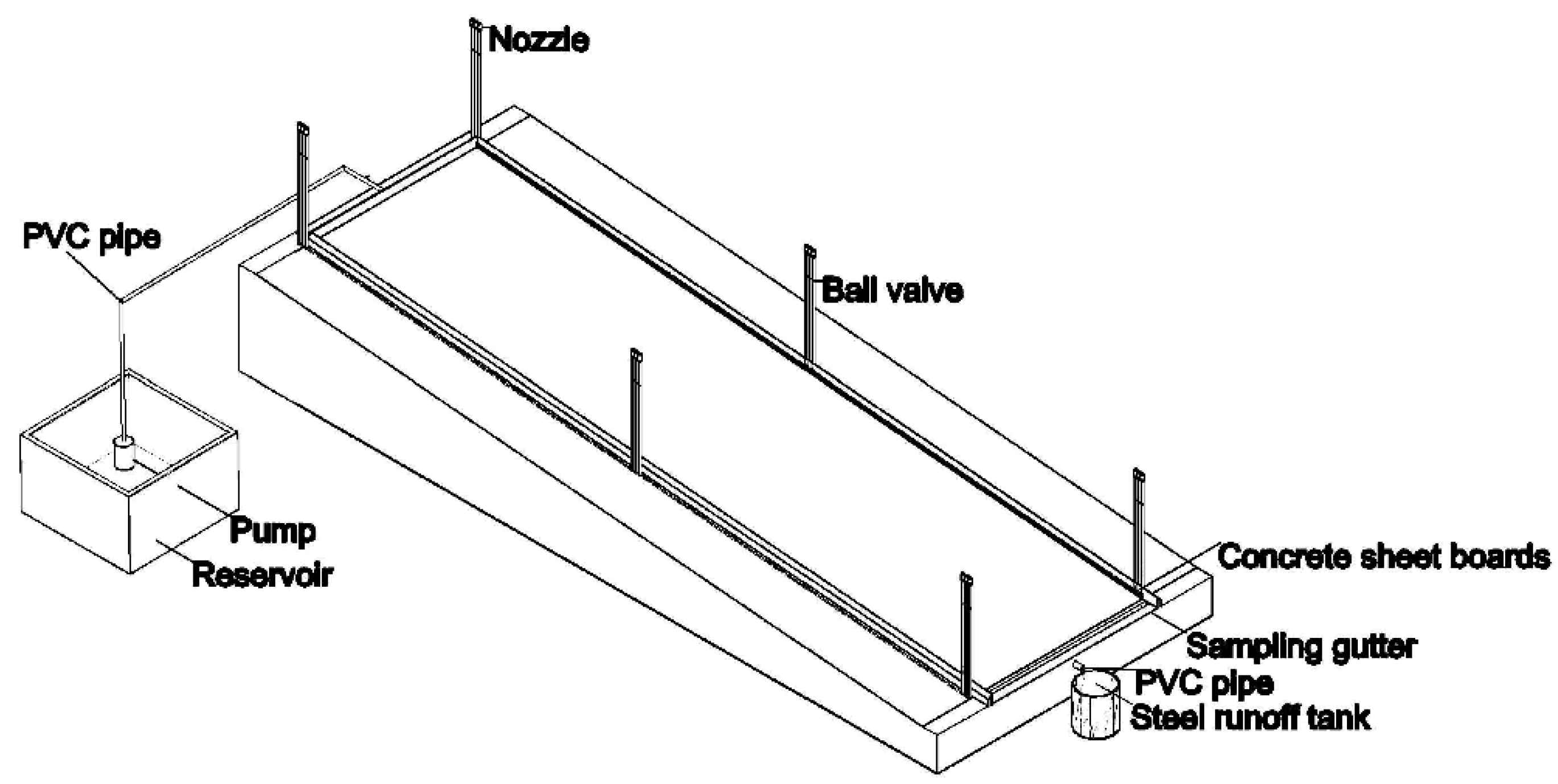
The rainfall simulation device was designed and manufactured by the college of water resources and civil engineering, China Agricultural University. Side-sprinkle simulators, which included 3 nozzles at every 5 m for each side, were used in the experiment. The simulator nozzles were 3.2 m above the soil surface with 180 degrees in the middle and 90 degrees at the four corners of the runoff plots. The effective rainfall area was 10.0 m × 5.0 m. The rainfall intensities and uniformity were measured by placing rainfall gauges on the slope prior to the experiments. The rainfall intensities were controlled by changing the number of nozzles and the nozzle aperture. A sketch of the slope and simulated rainfall system is shown in Figure 1. The error of the rainfall intensities should be under 5% of the designed rainfall intensities. The rainfall intensity ranged from 20 to 120 mm/h, and the uniformity was above 85%. The measured median raindrop diameter was 1.4 mm, and the calculated kinetic energy of rainfall was 13.52 J/(mm m). The local groundwater was employed as simulated rainfall water.

2.3. Experimental Procedure

Experimental treatments in the study included four slope gradients (5, 10, 15, and 20°) and three rainfall intensities (25, 50 and 75 mm/h). The tested slope was leveled with a spade and then left undisturbed for approximately two weeks. The application rate of the urea-N was 300 kg/ha according to the local fertilization application amount on the maize land. Before the experiment, 3.26 kg of the urea was dissolved by 50 L water. The urea solution was sprayed on the soil surface uniformly with a sprayer. After the completion of experiments at 75 mm/h, 30 cm of the surface soil was removed from the slope, and then the soil in the local site was backfilled under the soil bulk density of 1.45 g/cm³ to ensure the consistency of the physical and chemical soil properties. Then, the tested slope was levelled and left undisturbed until the beginning of the experiment at 50 mm/h. Before the start of the experiment at 25 mm/h, the above procedures were repeated. The experiments were carried out around 6 AM to eliminate the influences of wind. In order to ensure that the initial moisture content of each treatment was consistent, the slope was wetted with pre-wet treatment, which meant a constant rainfall intensity of 20 mm/h was applied on the experimental plot until the generation of runoff 12 h before the experiments. The soil moisture content of the surface soil (0–10 cm) was measured by the oven-dried method and the ammonium concentration of the surface soil was measured by indophenol-blue colorimetric methods using a spectrophotometer prior to the start of the experiment (Table 1).

The time to runoff was recorded for each rainfall event, and each rainfall simulation experiment lasted for 50 min. Runoff samples were collected at the outlet of the flume in a plastic bucket. After the initial time to runoff, the outflow samples were collected every 5 min and lasted for 1 min. The water heights of the runoff samples were measured to calculate the volume. Then, a 300 mL subsample was collected from the bucket until the completion of the precipitation and then transferred into a plastic bottle. The plastic bottles were stored at 4 °C in a refrigerator for chemical analysis. In the laboratory, the ammonium nitrogen concentrations were measured by standard colorimetric method.

2.4. Theoretical Analysis

2.4.1. Governing Equation

The kinematic wave equation has been widely used to describe water flow over a slope during rainfall. The mass conservation equation can be expressed as

$$\frac{\partial \mathrm{q}}{\partial \mathrm{x}}+\frac{\partial \mathrm{h}}{\partial \mathrm{t}}=\mathrm{r}-\mathrm{i}$$

(1)

where q(x, t) is unit discharge (cm²/min), h(x, t) is runoff depth (cm), x is the distance (cm) along the overland flow plane, t is time (min), i is infiltration rate (cm/min), and r is the rainfall intensity (cm/min).

The unit discharge of runoff is a function of overland flow depth:

$$\mathrm{q}=\frac{1}{\mathrm{n}}{\mathrm{J}}^{0.5}{\mathrm{h}(\mathrm{x},\mathrm{t})}^{5/3}$$

(2)

where $\mathrm{n}$ is the Manning’s coefficient (s/m^1/3), and $\mathrm{J}$ is the hydraulic gradient.

By assuming that overland-flow depth change is proportional to the rainfall excess, an approximate analytical solution for the kinematic wave equation can be expressed as [27]:

$$\frac{\partial \mathrm{h}}{\partial \mathrm{t}}=\mathrm{c}(\mathrm{r}-\mathrm{i})$$

(3)

where c is a coefficient. Then, the unit discharge q(x,t) can be described by

$$\mathrm{q}(\mathrm{x},\mathrm{t})=(1-\mathrm{c})(\mathrm{r}-\mathrm{i})\mathrm{x}$$

(4)

The boundary conditions of Equation (3) are

$$\mathrm{q}(\mathrm{x},0)=\mathrm{q}(0,\mathrm{t})=0$$

(5)

Based on the conception of diffusion, the solute mass conservation can be expressed as

$$\mathrm{h}\frac{\partial {\mathrm{C}}_{\mathrm{r}}}{\partial \mathrm{t}}+\mathrm{q}\frac{\partial {\mathrm{C}}_{\mathrm{r}}}{\partial \mathrm{x}}{=\mathrm{k}}_{\mathrm{m}}\left({\mathrm{C}}_{\mathrm{s}}{-\mathrm{C}}_{\mathrm{r}}\right){-\mathrm{rC}}_{\mathrm{r}}$$

(6)

$$\frac{\partial {\mathrm{h}}_{\mathrm{m}}{\mathrm{C}}_{\mathrm{s}}{(\mathsf{\theta }}_{\mathrm{s}}{+\mathsf{\rho }}_{\mathrm{s}}{\mathrm{k}}_{\mathrm{s}})}{\partial \mathrm{t}}{=\mathrm{k}}_{\mathrm{m}}\left({\mathrm{C}}_{\mathrm{r}}{-\mathrm{C}}_{\mathrm{s}}\right){+\mathrm{i}(\mathrm{C}}_{\mathrm{r}}{-\mathrm{C}}_{\mathrm{s}})$$

(7)

where ${\mathrm{h}}_{\mathrm{m}}$ is depth of the mixing layer (cm), ${\mathrm{C}}_{\mathrm{r}}$ is solute concentration in the runoff (mg/L), ${\mathrm{C}}_{\mathrm{s}}$ is solute concentration in the mixing layer (mg/L), ${\mathsf{\theta }}_{\mathrm{s}}$ is the saturated soil volumetric moisture content (cm³/cm³), ${\mathsf{\rho }}_{\mathrm{s}}$ is the soil bulk density (g/cm³), ${\mathrm{k}}_{\mathrm{s}}$ is solute adsorption coefficient (cm³/g), and ${\mathrm{k}}_{\mathrm{m}}$ is the mass transfer coefficient (cm/min).

2.4.2. Solution of the Surface Runoff Equation

The Philip’s formula [28] can be used to simulate the infiltration process of a soil surface under rainfall. Before the generation of runoff, the infiltration capacity is higher than the rainfall intensity and the infiltration rate is equal to the rainfall intensity. As time progresses, the infiltration rate gradually decreases and becomes less than rainfall intensity and the surface runoff is formed at the ponding time. The infiltration equation can be expressed as

$$\{\begin{array}{cc}\mathrm{i}=\mathrm{r}\hfill & \mathrm{t}\le {\mathrm{t}}_{\mathrm{p}}\hfill \\ \mathrm{i}=0.5\mathrm{S}{(\mathrm{t}-\Delta \mathrm{t})}^{-0.5}\hfill & {\mathrm{t}>\mathrm{t}}_{\mathrm{p}}\hfill \end{array}$$

(8)

where t_p is the time of ponding (min), S is the sorptivity (cm min^−1/2).t_p and $\Delta \mathrm{t}$ can be solved by the modified Philip equation, ${\mathrm{t}}_{\mathrm{p}}=\frac{{\mathrm{S}}^2}{{2\mathrm{r}}^2}$ and $\Delta \mathrm{t}=\frac{{\mathrm{S}}^2}{{4\mathrm{r}}^2}$.

By combining Equations (4) and (8), the unit discharge of runoff can be expressed as

$$\{\begin{array}{c}\mathrm{q}(\mathrm{x},\mathrm{t})=0\mathrm{t}\le {\mathrm{t}}_{\mathrm{p}}\\ \mathrm{q}(\mathrm{x},\mathrm{t})=(1-\mathrm{c})(\mathrm{r}-0.5\mathrm{S}{(\mathrm{t}-\Delta \mathrm{t})}^{-0.5})\mathrm{x}{\mathrm{t}>\mathrm{t}}_{\mathrm{p}}\end{array}$$

(9)

By combining Equations (2) and (9), the runoff depth can be expressed as

$$\mathrm{h}(\mathrm{x},\mathrm{t})=(\frac{1}{\mathrm{n}}{\mathrm{J}}^{0.5}{)}^{-0.6}{\left(\right(1-\mathrm{c}\left)\right(\mathrm{r}-0.5\mathrm{S}{(\mathrm{t}-\Delta \mathrm{t})}^{-0.5}\left)\mathrm{x}\right)}^{0.6}$$

(10)

2.4.3. Solution of the Solute Transport Equation

For turbulent flow, the mass transfer coefficient k_m can be determined by the film theory. It is assumed that the overland flow can be divided into two regions: a near-surface laminar layer and a turbulent, completely mixed layer. The mass transfer is supposed to driven by molecular diffusion. Then, the mass transfer coefficient k_m can be deduced by the hydraulic mechanics of the overland flow [26]. The mass transfer coefficient can be calculated by

$${\mathrm{k}}_{\mathrm{m}}=\frac{{\mathsf{\rho }\mathrm{gD}}_{\mathrm{w}}}{\mathsf{\mu }}{\mathrm{nR}}^{1/3}{\mathrm{J}}^{1/2}$$

(11)

where g is the acceleration of gravity (m²/s), ρ is the density of water (kg/m³), R is the hydraulic radius (cm), approximately equal to the runoff height, μ is the water viscosity (kg/m), and D_w is the solute diffusivity in water (cm²/h). Equation (11) indicates that the mass transfer coefficient k_m is proportional to the h^1/3. For simplicity, the solute concentration along the slope is assumed to be uniform. By substituting Equation (11) into Equations (6) and (7), we obtain the following:

$$\mathrm{h}\frac{{\mathrm{dC}}_{\mathrm{r}}}{\mathrm{dt}}=\frac{{\mathsf{\rho }\mathrm{gD}}_{\mathrm{w}}}{\mathsf{\mu }}{\mathrm{nh}}^{1/3}{\mathrm{J}}^{1/2}\left({\mathrm{C}}_{\mathrm{s}}{-\mathrm{C}}_{\mathrm{r}}\right){-\mathrm{rC}}_{\mathrm{r}}$$

(12)

$$\frac{{\mathrm{dh}}_{\mathrm{m}}{\mathrm{C}}_{\mathrm{s}}{(\mathsf{\theta }}_{\mathrm{s}}{+\mathsf{\rho }\mathrm{k}}_{\mathrm{s}})}{\partial \mathrm{t}}=\frac{{\mathsf{\rho }\mathrm{gD}}_{\mathrm{w}}}{\mathsf{\mu }}{\mathrm{nh}}^{1/3}{\mathrm{J}}^{1/2}\left({\mathrm{C}}_{\mathrm{r}}{-\mathrm{C}}_{\mathrm{s}}\right){+\mathrm{i}(\mathrm{C}}_{\mathrm{r}}{-\mathrm{C}}_{\mathrm{s}})$$

(13)

The solute concentration in the mixing layer before runoff can be calculated by [11]

$${\mathrm{C}(\mathrm{x},\mathrm{t}}_{\mathrm{p}})=\frac{{(\mathsf{\theta }}_{\mathrm{i}}{+\mathsf{\rho }}_{\mathrm{s}}{\mathrm{k}}_{\mathrm{s}}{)\mathrm{C}}_0}{{\mathsf{\theta }}_{\mathrm{s}}{+\mathsf{\rho }}_{\mathrm{s}}{\mathrm{k}}_{\mathrm{s}}}$$

(14)

where ${\mathsf{\theta }}_{\mathrm{i}}$ is the initial soil water content, and ${\mathrm{C}}_0$ is the initial solute concentration of the soil solution.

It is difficult to obtain the analytical solution of the ordinary differential equations. Thus, Equation (12) and Equation (13) are solved numerically using the Runge–Kutta–Fehlberg method by Matlab 12.0.

2.5. Data Analysis

Multivariate nonlinear regressions were made to determine parameters of the runoff model and the nutrient transport mode for each simulated rainfall event with the Matlab 2012 for Windows package. The coefficient of determination (R²) and root mean square error (RMSE) were applied to evaluate the agreement between the simulated results and experimental data in runoff and the nutrient transport process. R² and RMSE can be expressed as

$${\mathrm{R}}^2=1-\frac{{{\displaystyle \sum }}_{\mathrm{i}=1}^{\mathrm{n}}{{(\mathrm{o}}_{\mathrm{i}}{-\mathrm{p}}_{\mathrm{i}})}^2}{{{\displaystyle \sum }}_{\mathrm{i}=1}^{\mathrm{n}}{{(\mathrm{o}}_{\mathrm{i}}-\overline{{\mathrm{o}}_{\mathrm{i}}})}^2}$$

(15)

$$\mathrm{RMSE}=\sqrt{\frac{{{\displaystyle \sum }}_{\mathrm{i}=1}^{\mathrm{n}}{{(\mathrm{o}}_{\mathrm{i}}{-\mathrm{p}}_{\mathrm{i}})}^2}{\mathrm{n}}}$$

(16)

where $\mathrm{n}$ is the total number of the data, ${\mathrm{o}}_{\mathrm{i}}$ is the observed value at time $\mathrm{i}$, $\overline{{\mathrm{o}}_{\mathrm{i}}}$ is the average observed value, ${\mathrm{p}}_{\mathrm{i}}$ is the predicted value at time $\mathrm{i}$, and $\overline{{\mathrm{p}}_{\mathrm{i}}}$ is the average predicted value.

3. Results and Discussions

3.1. Effects of Slope Gradient and Rainfall Intensity on Runoff Process

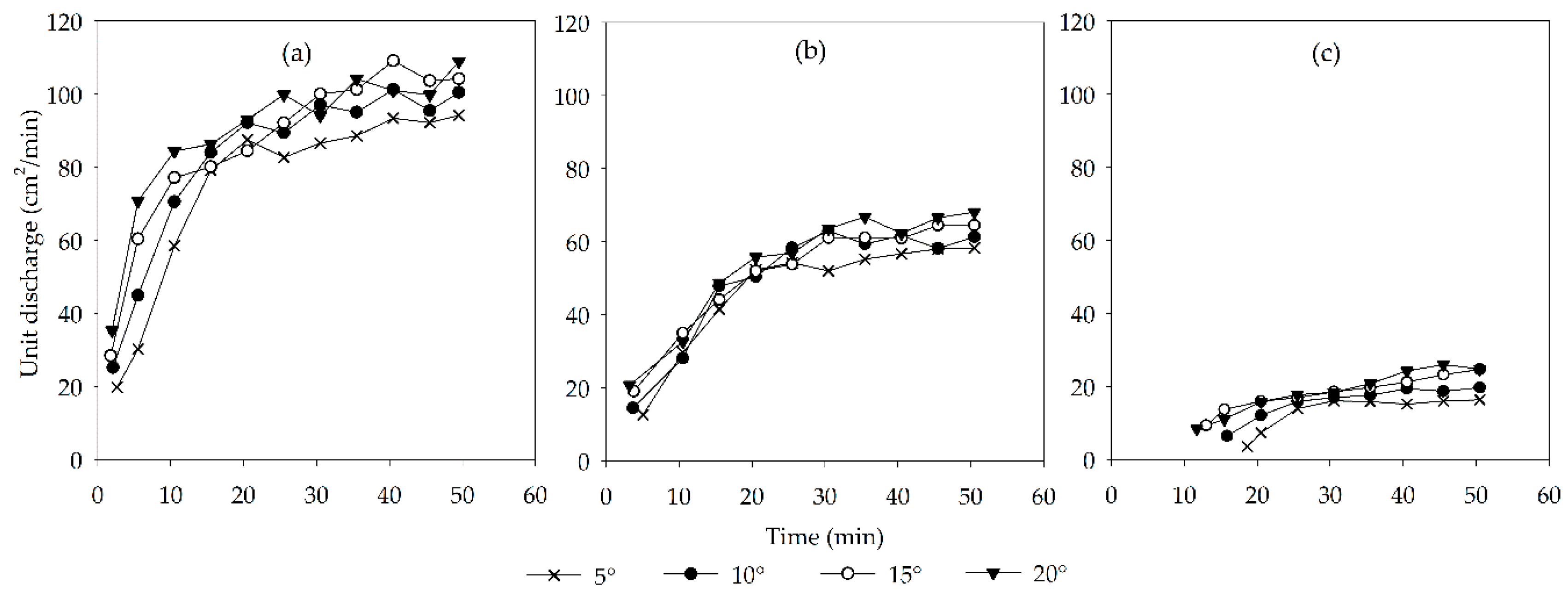
The runoff generation processes for different slopes under three rainfall intensities are shown in Figure 2. The unit discharge of runoff increased sharply after the generation of runoff and then tended to stabilize gradually over time. This was mainly due to the rapid decrease of the infiltration capacity of soil at the beginning of rainfall. As time progressed, the infiltration rate tended to be stable. The runoff processes were influenced by the rainfall intensity and slope gradient. From

Table 2. The variation of total runoff and ammonium nitrogen losses under different rain intensities and slope gradients.

Rainfall Intensity (mm/h)	Slope Gradient	Total Runoff (m3)	Total Ammonium Nitrogen Losses (mg NH4+-N)
75	5	1.82	2768
	10	2.01	5563
	15	2.11	7485
	20	2.18	9356
50	5	1.09	1468
	10	1.18	2252
	15	1.21	3341
	20	1.28	4141
25	5	0.23	457
	10	0.28	868
	15	0.35	1162
	20	0.37	1584

, it could be shown that the total runoff for slope gradients of 5°, 10°, 15° and 20° were 1.82, 2.01, 2.11 and 2.18 m³ under a rainfall intensity of 75 mm/h, respectively, indicating a higher runoff rate on a slope with a larger slope gradient. This phenomenon could also be observed under rainfall intensities of 50 mm/h and 25 mm/h. The results were in agreement with former research [29,30,31]. A possible explanation could be that as the slope steepens, more fine particles will be transported by overland flow, which may clog pores below the soil surface, thus reducing the infiltration capacity of steeper slopes [32]. The total runoff also increased with increasing rainfall intensities (Table 2), and runoff with larger rainfall intensities increased more quickly than for smaller rainfall intensities (Figure 2). From Table 2, it can be seen that the total runoff at a rainfall intensity of 75 mm/h was 6.9 times larger than that of 25 mm/h on a 5° slope, which was consistent with the results of Wei, et al. [33]. Generally, as rainfall intensity increased, the time to runoff was shorter. The infiltration rate more easily reached a stable state.

3.2. Effects of Slope Gradient and Rainfall Intensity on the Transport of Ammonium Nitrogen

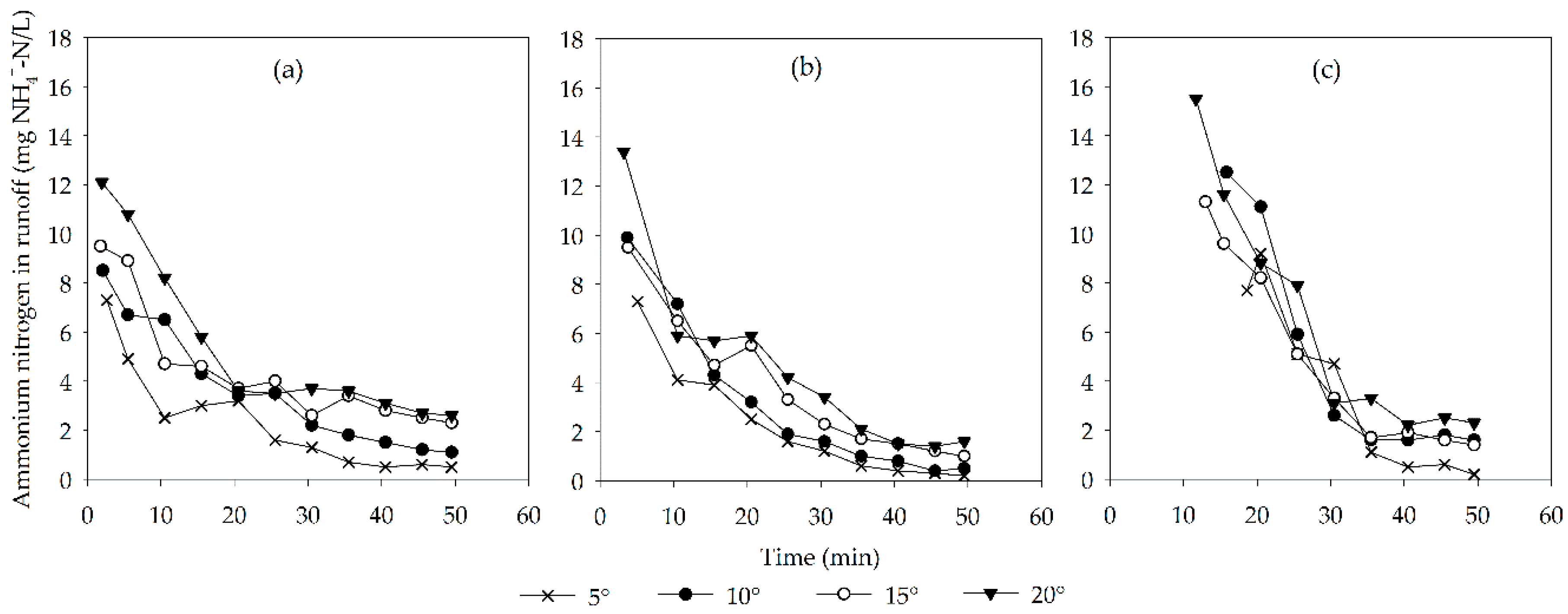
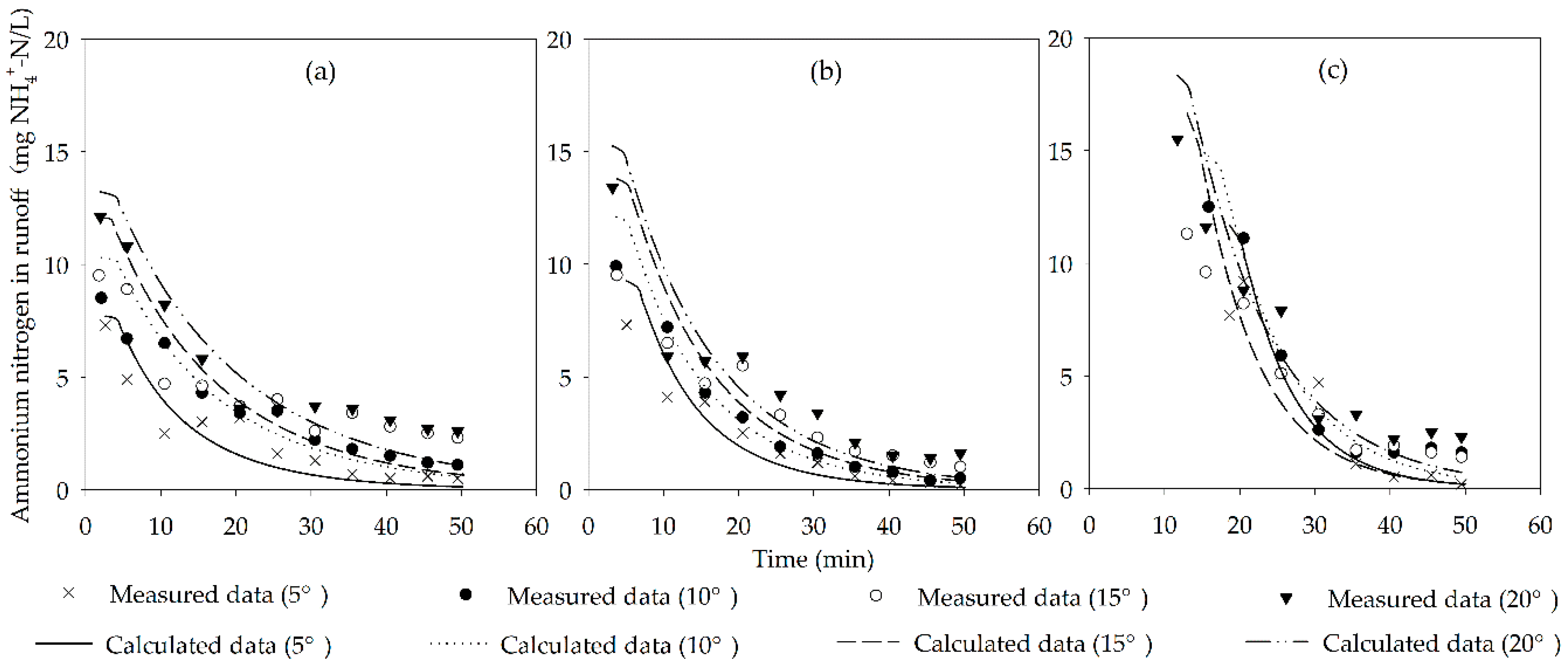
The effects of slope gradient and rainfall intensity on ammonium nitrogen concentration in the runoff are shown in Figure 3. The changing trends in ammonium nitrogen transport to runoff had a very similar pattern. The ammonium nitrogen concentration tended to reach the maximum value after a short period of the initial time to runoff, then it tended to decrease with time, and finally it became relatively stable. The reason for the results might be that during the initial stage of rainfall, the infiltration capacity was larger than the rainfall intensity, so the nutrient in the mixing layer was carried down to the deeper soil layer by the rain water, which resulted in a continuous decrease of the nutrient concentration in the mixing layer. As time progressed, the nutrient in the mixing layer began to transport to the runoff through the effects of diffusion at the moment that the ponded water occurred. After a very short time, the nutrient concentration would reach the maximum value [34,35]. Then, the difference of the concentration between the mixing layer and runoff decreased with time, which indicated the decreasing trend of the nutrient concentration in the runoff.

The slope gradient had effects on the processes of ammonium nitrogen transport to runoff. Larger ammonium nitrogen concentration could be observed in the larger slope gradient. The initial ammonium nitrogen concentrations were 7.3, 8.5, 9.5 and 12.1 mg/L for slope gradients of 5, 10, 15 and 20° under a rainfall intensity of 75 mm/h, respectively. The total ammonium nitrogen losses for slope gradients of 5, 10, 15 and 20° were 2768, 5563, 7485, 9356 mg for 75 mm/h, respectively (Table 2). The results might be due to the fact that the infiltration capacity of the greater slope gradient plot is smaller than that of the smaller gradient plot, which leads to a shorter time to form runoff. It has been reported that the time to runoff significantly affects the solute transport processes [17]. Because of the shorter time to runoff, the amount of nutrient leaching was smaller for the greater slope gradient plot, indicating a higher initial nutrient concentration. Moreover, the overland flow velocity of the larger slope gradient was generally greater than that of the smaller gradient, which would result in more turbulent flow [27,36]. The turbulent flow would increase the possibility for the nutrient transport into the runoff, which could possibly explain the higher ammonium nitrogen for larger slope gradients during the decreasing and stable stages of ammonium nitrogen loss processes.

The processes of ammonium nitrogen transport to runoff would also be affected by the rainfall intensities. The initial ammonium nitrogen concentrations at 20° were 12.1 mg/L, 13.4 mg/L and 15.5 mg/L for 75, 50 and 25 mm/h, respectively, indicating a decreasing trend with an increase of rainfall intensity. However, the total amount of ammonium nitrogen losses increased with an increase of rainfall intensity (Table 2). The nutrient transport to runoff is mainly determined by the nutrient concentration of the soil surface and the diffusion effects between the soil surface and runoff. Higher rainfall intensities will dilute the nutrient in the mixing layer more quickly than lower rainfall intensities, which will reach a balance between the mixing layer and runoff faster, resulting in a more rapid time to reach a steady state in nutrient concentration. The decreasing trend of initial nutrient concentration with increasing rainfall intensities was in agreement with the results of Xiao, et al. [37]. This might be caused by the fact that although higher rainfall intensity would certainly increase the possibility for nutrient transport to runoff, the dilution effects of runoff to nutrients would be another dominant factor during nutrient loss processes under a relatively small soil solution situation.

3.3. Parameter Estimation

The parameters used in this model include the soil properties parameters, hydraulic parameters and nutrient transport parameters. Some of these parameters could be measured directly. For example, the soil bulk density (ρ_s), the initial water content (θ_i) and the saturated soil water content (θ_s) are all listed in Table 1. The adsorption isotherm of ammonium nitrogen for the experimental soil was obtained based on the isothermal linear adsorption method [37], namely 1.74 cm³/g. The molecular diffusion coefficient in free water (D_w) for ammonium nitrogen is assigned to be 0.063 cm²/h [38]. The Manning coefficient (n) is assigned to be 0.017 s/m^1/3 for the slope tested in this experiment. The water viscosity μ is 1.05 × 10⁻³ kg/(m s) at 20 °C. The initial ammonium nitrogen concentrations of soil solution were measured directly and are shown in Table 1. The time to runoff, t_p, was measured directly during the simulated rainfall (

Table 3. The initial time to runoff (t_p), adsorptivity (S), R² and RMSE obtained by curve-fitting the results of the runoff model under different rainfall intensities and slope gradients.

Designed Rainfall Intensities	Slope Gradient	tp (min)	S (cm/min1/2)	c	R2	RMSE (cm2/min)
75	5	2.15	0.26	0.15	0.94	8.12
	10	1.60	0.22	0.12	0.96	6.89
	15	1.28	0.20	0.10	0.96	6.52
	20	1.45	0.21	0.06	0.99	3.93
50	5	4.57	0.25	0.10	0.98	2.95
	10	3.17	0.21	0.11	0.93	5.32
	15	3.28	0.21	0.05	0.95	4.58
	20	2.70	0.19	0.08	0.92	5.99
25	5	18.15	0.25	0.13	0.87	2.75
	10	15.35	0.23	0.10	0.92	2.55
	15	12.50	0.21	0.05	0.89	3.44
	20	11.20	0.20	0.06	0.94	2.40

).

However, there are some parameters that could not be measured directly, such as the soil hydraulic parameters, S and c, and the depth of the mixing layer, h_m. The hydraulic parameters, S and c, could be estimated by the curve-fitting of the established runoff model (Equation (9)). The depth of the mixing layer under different rainfall intensities and slope gradient, h_m, was determined by the curve-fitting method of the solute mass conversation model (Equations (12) and (13)). Parameters deduced by the curve-fitting method could be regarded as the best match between measured data and experimental data. However, these parameters could be influenced by many factors. For this experiment, rainfall intensity and slope gradient are the two dominant factors. In order to establish an ammonium nitrogen transportation model which can be applied to the experimental site, the effects of rainfall intensity and slope gradient on these parameters (t_p, S, c, h_m) were analyzed.

3.4. Modeling Runoff Processes and Ammonium Nitrogen Concentration in Overland Flow

3.4.1. Modeling Runoff Processes

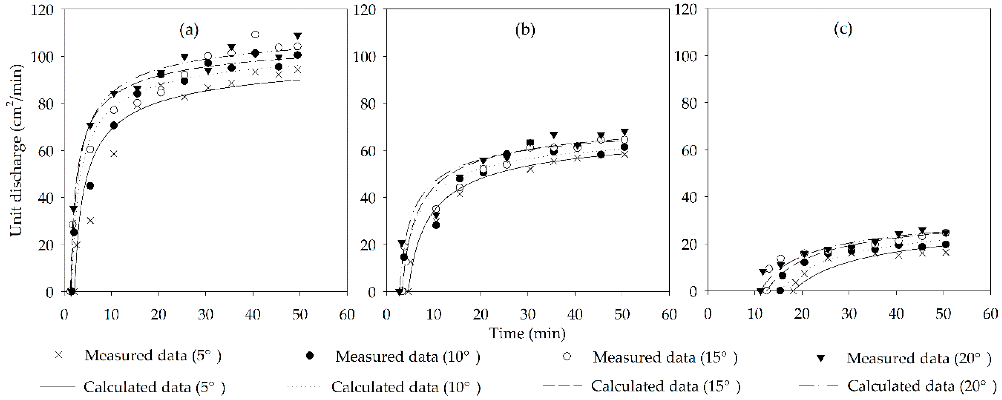
The runoff processes were simulated by Equation (9). The curve-fitting results of the runoff model are shown in Table 3 and Figure 4. The R² and RMSE ranged from 0.87 to 0.99 and 2.40 to 8.12 cm²/min, respectively. It could be concluded that the established runoff model based on Philip’s infiltration equation could accurately describe the runoff processes. In this runoff model, the time to runoff (t_p), adsorptivity (S) and coefficient (c) are the three parameters which can determine the runoff processes with a given rainfall intensity and slope gradient. It could be shown that time to runoff (t_p) decreased with an increase of rainfall intensity and slope gradient despite the fact that the t_p at 20° was larger than that at 15° under a rainfall intensity of 75 mm/h. The results were mainly due to the smaller infiltration capacity of the larger gradient. A larger rainfall intensity would surely accelerate the saturation processes of the slope soil. The t_p was then fitted with the exponential function. The R² was 0.997, indicating the relationship among t_p and slope gradient, and the rainfall intensity could be described by the exponential function. The relationships could be expressed as

$${\mathrm{t}}_{\mathrm{p}}=4.65{\times 10}^{-4}{\mathrm{r}}^{-2.03}{\mathrm{G}}^{-0.34}{\mathrm{R}}^2=0.997\mathrm{n}=12$$

(17)

where G is the slope gradient.

The combination of S and c were important factors that determined the shape of the runoff processes. As can be seen in

Table 4. The mixing depth (h_m), R² and RMSE obtained by curve-fitting the results of the solute transport model under different rainfall intensities and slope gradients.

Designed Rainfall Intensity (mm/h)	Slope Gradient	hm (cm)	R2	RMSE (mg/L)
75	5	0.20	0.89	0.92
	10	0.30	0.96	1.04
	15	0.31	0.92	1.63
	20	0.38	0.96	1.14
50	5	0.14	0.95	0.89
	10	0.18	0.99	0.73
	15	0.20	0.92	1.73
	20	0.22	0.92	1.56
25	5	0.07	0.90	1.67
	10	0.10	0.96	1.07
	15	0.08	0.94	2.45
	20	0.12	0.96	1.78

, the S decreased with an increase of slope gradient, while there was little difference under different rainfall intensities. The c decreased with an increase of slope gradient and rainfall intensity. The results were similar to the results of Yang et al. [11]. The results indicated that the increasing speed of the runoff under higher rainfall intensities and slope gradients was larger than that of lower rainfall intensities and slope gradients, which was discussed in Section 3.1. Then, the exponential function was applied to fit the results. The R² values were 0.895 and 0.678, respectively. The relationships could be expressed as

$$\mathrm{S}=0.33{\mathrm{r}}^{-0.0044}{\mathrm{G}}^{-0.18}{\mathrm{R}}^2=0.895\mathrm{n}=12$$

(18)

$$\mathrm{c}=0.71{\mathrm{r}}^{0.19}{\mathrm{G}}^{-0.47}{\mathrm{R}}^2=0.678\mathrm{n}=12$$

(19)

3.4.2. Modelling Ammonium Nitrogen Concentrations in Runoff.

From Figure 5, it can be seen that the proposed model overestimated the nutrient concentration in the early runoff time but underestimated the nutrient concentration in the later nutrient transport stage. As described in Section 3.2, after the start of simulated rainfall, the nutrient in the surface profile began to be carried down into the deep soil layer. When ponded water occurred, the nutrient began to transport into the runoff through diffusion effects. Because the nutrient concentration at the moment ponded water formed was very difficult to measure directly, the initial soil solution concentration was calculated by Equation (14). Without considering the leaching processes of the nutrient, the assigned initial soil solution concentration might be larger than the exact concentration, which might cause the overprediction of the initial concentration. Moreover, the proposed model only considered the diffusion processes without considering the raindrop dispersion effects before the generation of runoff. It has been reported that the raindrop effects remain constant until some critical flow depth, and then decrease with flow depth as a power function [39,40]. This meant that the proposed model might underestimate the mass transfer coefficient, which resulted in an underestimation of the nutrient concentration during the later steady stage.

From Table 4, it can be seen that the R² and RMSE ranged from 0.87 to 0.99 and 2.40 to 8.12 mg/L, respectively, indicating that the nutrient transport into the runoff could be simulated by the proposed model. The depth of the exchange layer (h_m) and mass transfer coefficient were two important parameters to determine the accuracy of this model. It has been reported that the depth of the exchange layer ranged between 2 mm and 3 mm [13,41]. Li et al. [25] conducted a field experiment to simulate the ammonium nitrogen and nitrate nitrogen transport processes. The results showed that the depth of the exchange layer, which was influenced by the rainfall intensity and slope gradient, was between 0.4 cm and 0.6 cm. The results of Yang, et al. [42] indicated that the depth of the interaction zone increased with an increase of rainfall intensity and slope gradient, which was similar to our results. The mixing depth ranged from 0.08–0.38 cm, which increased with increasing slope gradients and rainfall intensities despite the fact that the mixing depth of 15° was smaller than that of 10° under a rainfall intensity of 25 mm/h. Then, the exponential function was applied to fit the results. The R² was 0.981. The relationships could be expressed as

$${\mathrm{h}}_{\mathrm{m}}=14.82{\mathrm{r}}^{1.11}{\mathrm{G}}^{0.39}{\mathrm{R}}^2=0.981\mathrm{n}=12$$

(20)

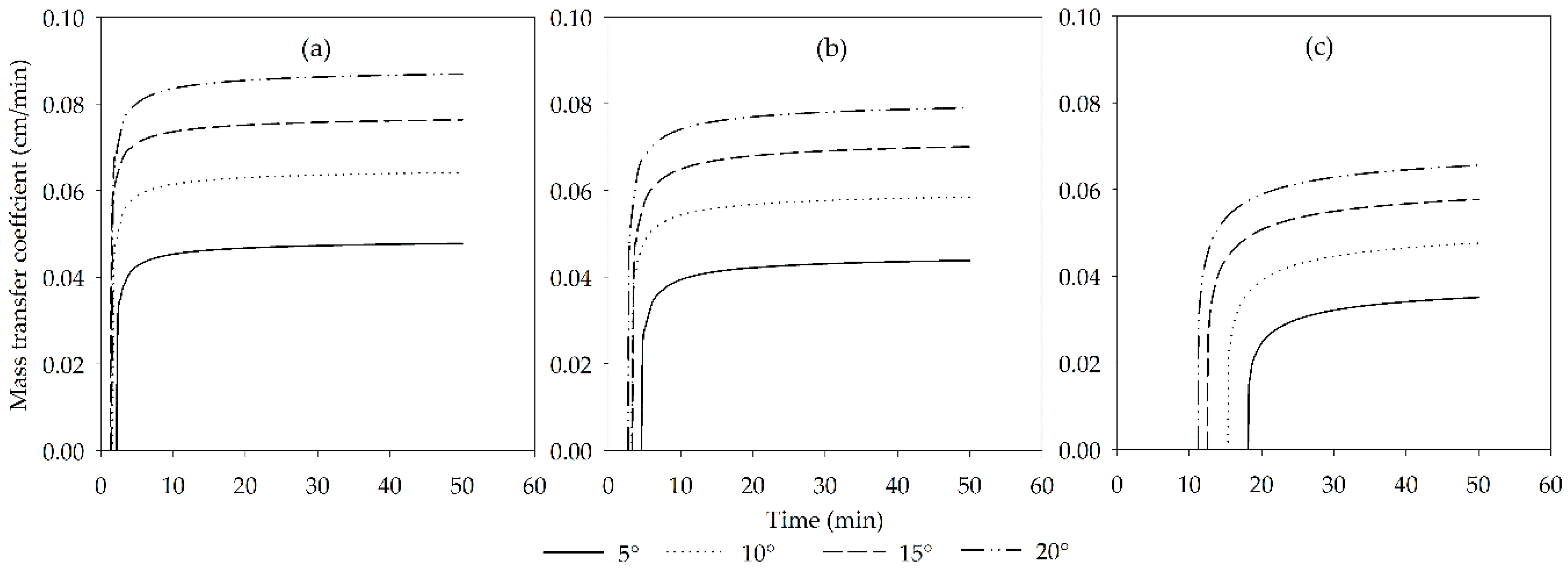
The mass transfer coefficient changes over time are shown in Figure 6. The mass transfer coefficient increased sharply after the generation of runoff and then tended to be stable. The results indicated that without considering the effects of raindrop dispersion, there was no nutrient transport into the surface runoff, which meant that the nutrient transport into the surface runoff occurred with the disturbance of overland flow. The mass transfer coefficient increased with slope gradients and rainfall intensities, ranging from 0 to 0.087 cm/min. The mass transfer coefficient could be affected by many factors, such as rainfall intensity, soil type and soil surface cover. A laboratory experiment has been conducted to study the rainfall-induced chemical transport from soil to runoff [21]. The results showed that the mass transfer coefficient increased with an increase of rainfall intensity, namely 0.76, 0.54 and 0.32 cm/h under rainfall intensities of 75.6, 50.4 and 28.8 mm/h, respectively. Tao, Wu and Wang [35] reported that the mass transfer coefficient ranged from 0.04 to 0.12 cm/min under different rainfall patterns. The mass transfer coefficient of larger rainfall intensities also had a relatively large value compared with the smaller rainfall intensities, while for different soil types, the mass transfer coefficient of the clay texture was largest when compared with that of loam and fine sandy loam. This was similar to the results of Dong and Wang [43]. Dong, et al. [44] conducted an experiment on a loessial slope with three levels of stone covers. It turned out that the mass transfer coefficient decreased with an increase of the area of stone cover. With all of these factors taken into consideration, it has been concluded that a mass transfer coefficient ranging from 0.9 cm/h to 6.8 cm/h was appropriate [45].

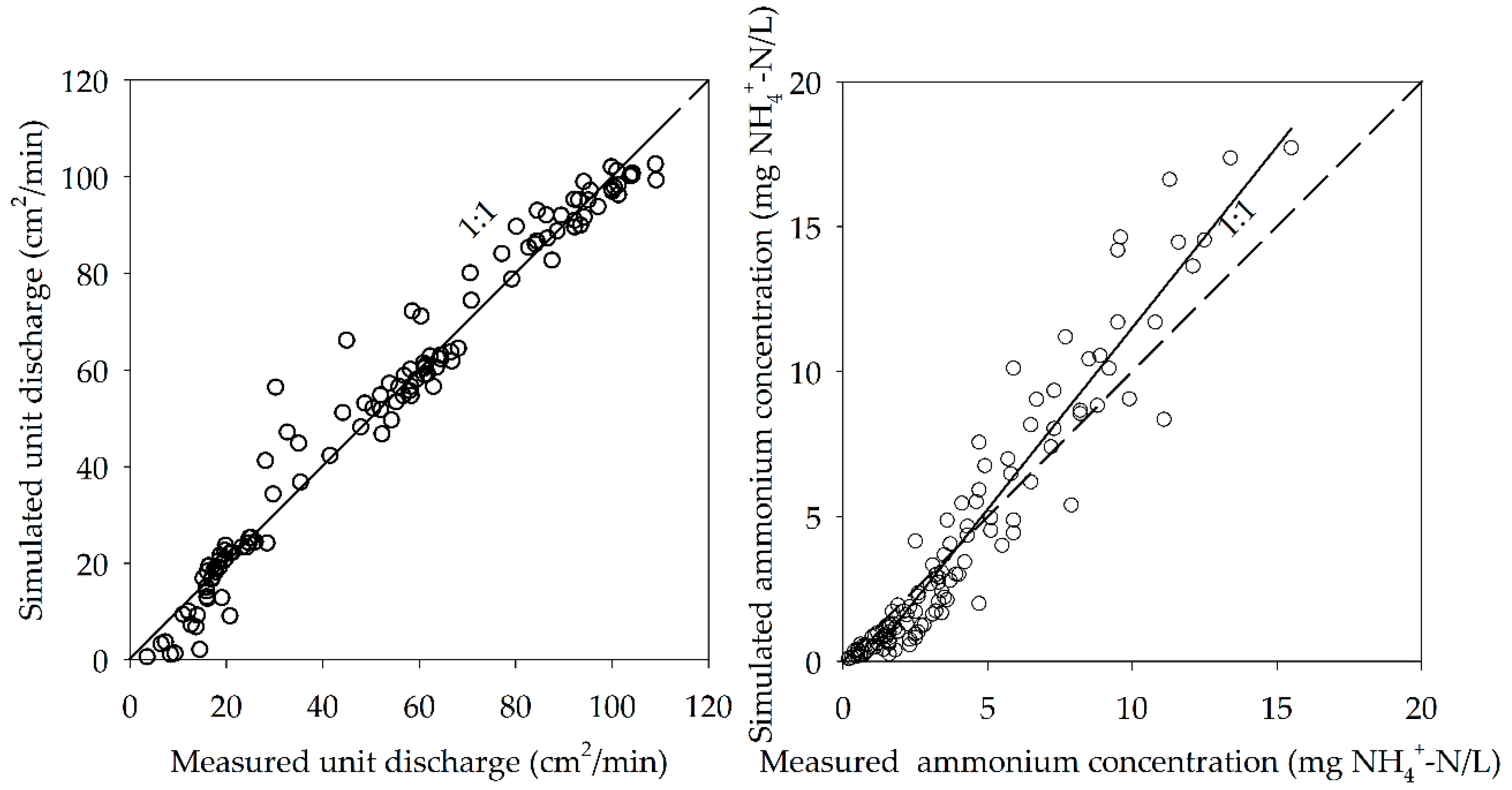
Overall, with the combination of Equations (9,10,12–14,17–20), a diffusion-based model with a time-dependent mass transfer coefficient has been established to predict the ammonium nitrogen transport processes at the experimental site under different slope gradients and rainfall intensities. As shown in Figure 7, the model could fit the experimental data well, indicating that the proposed model could be used to predict the nutrient transport to runoff processes in the experimental site.

4. Conclusions

On the basis of Wallach’s theory [26], a mathematical model of solute transport from soil solution to overland flow with a time-dependent mass transfer coefficient was established. This was examined with four slope gradients (5°, 10°, 15° and 20°) and three rainfall intensities (75, 50 and 25 mm/h). The results showed that the unit discharge of runoff first increased sharply with time and then tended to be stable, while the ammonium nitrogen in runoff first decreased rapidly and then tended to reach a stable state. The unit discharge of runoff increased with an increase of slope gradient and rainfall intensity, and the ammonium nitrogen increased with an increase of slope gradient. The runoff processes and ammonium nitrogen in runoff could be well described by the proposed model. Furthermore, the relationships among parameters obtained by curve-fitting the results of slope gradient and rainfall intensity were analyzed, which was able to provide a method to predict the runoff processes and nutrient loss in runoff at the experimental site under different slope gradients and rainfall intensities. The applicability of the model for different locations needs to be further evaluated. The proposed model does not take the leaching process and raindrop dispersion effects into consideration. Our further research may focus on adding these two processes into the model.

References

- Vadas, P.A.; Powell, J.M. Monitoring nutrient loss in runoff from dairy cattle lots. Agric. Ecosyst. Environ. 2013, 181, 127–133. [Google Scholar] [CrossRef]
- Ramos, M.; Benito, C.; Martínez-Casasnovas, J. Simulating soil conservation measures to control soil and nutrient losses in a small, vineyard dominated, basin. Agric. Ecosyst. Environ. 2015, 213, 194–208. [Google Scholar] [CrossRef]
- Parris, K. Impact of agriculture on water pollution in OECD countries: Recent trends and future prospects. Int. J. Water Resour. Dev. 2011, 27, 33–52. [Google Scholar] [CrossRef]
- Sharpley, A.; Moyer, B. Phosphorus forms in manure and compost and their release during simulated rainfall. J. Environ. Qual. 2000, 29, 1462–1469. [Google Scholar] [CrossRef]
- Wilson, G.; McGregor, K.; Boykin, D. Residue impacts on runoff and soil erosion for different corn plant populations. Soil Tillage Res. 2008, 99, 300–307. [Google Scholar] [CrossRef]
- Howarth, R.W.; Sharpley, A.; Walker, D. Sources of nutrient pollution to coastal waters in the United States: Implications for achieving coastal water quality goals. Estuaries 2002, 25, 656–676. [Google Scholar] [CrossRef]
- Kleinman, P.J.; Srinivasan, M.; Dell, C.J.; Schmidt, J.P. Role of rainfall intensity and hydrology in nutrient transport via surface runoff. J. Environ. Qual. 2006, 35, 1248. [Google Scholar] [CrossRef]
- Snyder, J.K.; Woolhiser, D.A. Effects of infiltration on chemical transport into overland flow. Trans. ASAE 1985, 28, 1450–1457. [Google Scholar] [CrossRef]
- Wallach, R.; Shabtai, R. Surface runoff contamination by chemicals initially incorporated below the soil surface. Water Resour. Res. 1993, 29, 697–704. [Google Scholar] [CrossRef]
- Srinivasan, M.; Kleinman, P.; Sharpley, A.; Buob, T.; Gburek, W. Hydrology of small field plots used to study phosphorus runoff under simulated rainfall. J. Environ. Qual. 2007, 36, 1833. [Google Scholar] [CrossRef] [PubMed]
- Yang, T.; Wang, Q.; Wu, L.; Zhao, G.; Liu, Y.; Zhang, P. A mathematical model for soil solute transfer into surface runoff as influenced by rainfall detachment. Sci. Total Environ. 2016, 557, 590–600. [Google Scholar] [CrossRef] [PubMed]
- Shi, X.; Wu, L.; Chenc, W.; Wang, Q. Solute Transfer from the Soil Surface to Overland Flow: A Review. Soil Sci. Soc. Am. J. 2011, 75, 1214. [Google Scholar] [CrossRef]
- Ahuja, L.; Sharpley, A.; Yamamoto, M.; Menzel, R. The depth of rainfall-runoff-soil interaction as determined by 32P. Water Resour. Res. 1981, 17, 969–974. [Google Scholar] [CrossRef]
- Steenhuis, T.; Walter, M. Closed form solution for pesticide loss in runoff water. Trans. ASAE 1980, 23, 0615–0620. [Google Scholar] [CrossRef]
- Ahuja, L.; Lehman, O. The extent and nature of rainfall-soil interaction in the release of soluble chemicals to runoff. J. Environ. Qual. 1983, 12, 34–40. [Google Scholar] [CrossRef]
- Havis, R.; Smith, R.; Adrian, D. Partitioning solute transport between infiltration and overland flow under rainfall. Water Resour. Res. 1992, 28, 2569–2580. [Google Scholar] [CrossRef]
- Walton, R.; Volker, R.; Bristow, K.L.; Smettem, K. Solute transport by surface runoff from low-angle slopes: Theory and application. Hydrol. Process. 2000, 14, 1139–1158. [Google Scholar] [CrossRef]
- Yang, T.; Wang, Q.J.; Liu, Y.L.; Zhang, P.Y.; Wu, L.S. A comparison of mathematical models for chemical transfer from soil to surface runoff with the impact of rain. Catena 2016, 137, 191–202. [Google Scholar] [CrossRef]
- Wallach, R.; Jury, W.A.; Spencer, W.F. Transfer of chemicals from soil solution to surface runoff: A diffusion-based soil model. Soil Sci. Soc. Am. J. 1988, 52, 612–618. [Google Scholar] [CrossRef]
- Chen, X.R.; Jia, J.D.; Gao, W.L.; Ren, Y.Z.; Tao, S. Selection of an index system for evaluating the application level of agricultural engineering technology. Pattern Recogn. Lett. 2018, 109, 12–17. [Google Scholar] [CrossRef]
- Gao, B.; Walter, M.T.; Steenhuis, T.S.; Hogarth, W.L.; Parlange, J.-Y. Rainfall induced chemical transport from soil to runoff: Theory and experiments. J. Hydrol. 2004, 295, 291–304. [Google Scholar] [CrossRef]
- Hairsine, P.; Rose, C. Rainfall detachment and deposition: Sediment transport in the absence of flow-driven processes. Soil Sci. Soc. Am. J. 1991, 55, 320–324. [Google Scholar] [CrossRef]
- Walker, J.D.; Walter, M.T.; Parlange, J.-Y.; Rose, C.W.; Tromp-van Meerveld, H.; Gao, B.; Cohen, A.M. Reduced raindrop-impact driven soil erosion by infiltration. J. Hydrol. 2007, 342, 331–335. [Google Scholar] [CrossRef]
- Walter, M.T.; Gao, B.; Parlange, J.-Y. Modeling soil solute release into runoff with infiltration. J. Hydrol. 2007, 347, 430–437. [Google Scholar] [CrossRef]
- Li, J.; Tong, J.; Xia, C.; Hu, B.X.; Zhu, H.; Yang, R.; Wei, W. Numerical simulation and experimental study on farmland nitrogen loss to surface runoff in a raindrop driven process. J. Hydrol. 2017, 549, 754–768. [Google Scholar] [CrossRef]
- Wallach, R.; Jury, W.A.; Spencer, W.F. The concept of convective mass transfer for prediction of surface-runoff pollution by soil surface applied chemicals. Trans. ASAE 1989, 32, 0906–0912. [Google Scholar] [CrossRef]
- Yang, T.; Wang, Q.J.; Su, L.J.; Wu, L.S.; Zhao, G.X.; Liu, Y.L.; Zhang, P.Y. An Approximately Semi-Analytical Model for Describing Surface Runoff of Rainwater Over Sloped Land. Water Resour. Manag. 2016, 30, 3935–3948. [Google Scholar] [CrossRef]
- Philip, J. The theory of infiltration: 1. The infiltration equation and its solution. Soil Sci. 1957, 83, 345–358. [Google Scholar] [CrossRef]
- Jiang, F.S.; Huang, Y.H.; Wang, M.K.; Lin, J.S.; Gan, Z.; Ge, H.L. Effects of Rainfall Intensity and Slope Gradient on Steep Colluvial Deposit Erosion in Southeast China. Soil Sci. Soc. Am. J. 2014, 78, 1741. [Google Scholar] [CrossRef]
- Poesen, J. The Role of Slope Angle in Surface Seal Formation. In International Geomorphology 1986, Part II; Wiley: Hoboken, NJ, USA, 1987; pp. 437–448. [Google Scholar]
- Ribolzi, O.; Patin, J.; Bresson, L.M.; Latsachack, K.O.; Valentin, C. Impact of slope gradient on soil surface features and infiltration on steep slopes in northern Laos. Geomorphology 2014, 127, 53–63. [Google Scholar] [CrossRef]
- Assouline, S.; Ben-Hur, M. Effects of rainfall intensity and slope gradient on the dynamics of interrill erosion during soil surface sealing. Catena 2006, 66, 211–220. [Google Scholar] [CrossRef]
- Wei, W.; Jia, F.; Lei, Y.; Chen, L.; Zhang, H.; Yang, Y. Effects of surficial condition and rainfall intensity on runoff in a loess hilly area, China. J. Hydrol. 2014, 513, 115–126. [Google Scholar] [CrossRef] [Green Version]
- Walton, R.; Volker, R.; Bristow, K.L.; Smettem, K. Experimental examination of solute transport by surface runoff from low-angle slopes. J. Hydrol. 2000, 233, 19–36. [Google Scholar] [CrossRef]
- Tao, W.; Wu, J.; Wang, Q. Mathematical model of sediment and solute transport along slope land in different rainfall pattern conditions. Sci. Rep. 2017, 7, 44082. [Google Scholar] [CrossRef] [Green Version]
- Peng, W.; Zhang, Z.; Zhang, K. Hydrodynamic characteristics of rill flow on steep slopes. Hydrol. Process. 2015, 29, 3677–3686. [Google Scholar] [CrossRef]
- Xiao, S.Q.; Yao, M.W.; Gao, W.B.; Su, Z.; Yao, X. Significantly enhanced dielectric constant and breakdown strength in crystalline@amorphous core-shell structured SrTiO3 nanocomposite thick films. J. Alloy Compd. 2018, 762, 370–377. [Google Scholar] [CrossRef]
- Weast, R.C. CRC Handbook of Chemistry and Physics, 55th Ed. (1974–1975) ed; CRC Press: Cleveland, OH, USA, 1974. [Google Scholar]
- Gao, B.; Walter, M.T.; Steenhuis, T.S.; Parlange, J.Y.; Nakano, K.; Rose, C.W.; Hogarth, W.L. Investigating ponding depth and soil detachability for a mechanistic erosion model using a simple experiment. J. Hydrol. 2003, 277, 116–124. [Google Scholar] [CrossRef]
- Proffitt, A.P.B.; Rose, C.W.; Hairsine, P.B. Rainfall Detachment and Deposition: Experiments with Low Slopes and Significant Water Depths. Soil Sci. Soc. Am. J. 1991, 55, 325–332. [Google Scholar] [CrossRef]
- Zhang, X.C.; Norton, L.D. Coupling mixing zone concept with convection-diffusion equation to predict chemical transfer to surface runoff. Trans. ASAE 1999, 42, 987–994. [Google Scholar] [CrossRef]
- Yang, T.; Wang, Q.; Xu, D.; Lv, J. A method for estimating the interaction depth of surface soil with simulated rain. Catena 2015, 124, 109–118. [Google Scholar] [CrossRef]
- Dong, W.; Wang, Q. Modeling Soil Solute Release into Runoff and Transport with Runoff on a Loess Slope. J. Hydrol. Eng. 2013, 18, 527–535. [Google Scholar] [CrossRef]
- Dong, W.; Song, C.; Qiang, F.; Wang, Q.; Cao, C. Modeling soil solute release and transport in runoff on a loessial slope with and without surface stones. Hydrol. Process. 2018, 32, 1391–1400. [Google Scholar] [CrossRef]
- Rumynin, V.G. Overland Flow Dynamics and Solute Transport; Springer Nature Switzerland AG: Basel, Switzerland, 2015; Volume 26. [Google Scholar] [CrossRef]
Figure 1.
Sketch of the slope and simulated rainfall system.
Figure 2.
Unit discharge of runoff over rainfall time under different slope gradients and different rainfall intensities: (a) 75 mm/h, (b) 50 mm/h, (c) 25 mm/h.
Figure 3.
The ammonium nitrogen (NH4+-N) concentration in runoff over rainfall time under different slope gradients and different rainfall intensities: (a) 75 mm/h, (b) 50 mm/h (c) 25 mm/h.
Figure 4.
Comparison of the calculated and measured unit discharge of runoff under different slope gradients and different rainfall intensities: (a) 75 mm/h, (b) 50 mm/h, (c) 25 mm/h.
Figure 5.
Comparison of the calculated and experimental ammonium nitrogen (NH4+-N) concentration in the runoff under different slope gradients and different rainfall intensities: (a) 75 mm/h, (b) 50 mm/h, (c) 25 mm/h.