Impacts of Introducing Remote Sensing Soil Moisture in Calibrating a Distributed Hydrological Model for Streamflow Simulation

Abstract

With the increased availability of remote sensing products, more hydrological variables (e.g., soil moisture and evapotranspiration) other than streamflow data are introduced into the calibration procedure of a hydrological model. However, how the incorporation of these hydrological variables influences the calibration results remains unclear. This study aims to analyze the impact of remote sensing soil moisture data in the joint calibration of a distributed hydrological model. The investigation was carried out in Qujiang and Ganjiang catchments in southern China, where the Dem-based Distributed Rainfall-runoff Model (DDRM) was calibrated under different calibration schemes where the streamflow data and the remote sensing soil moisture are assigned to different weights in the objective function. The remote sensing soil moisture data are from the SMAP L3 soil moisture product. The results show that different weights of soil moisture in the objective function can lead to very slight differences in simulation performance of soil moisture and streamflow. Besides, the joint calibration shows no apparent advantages in terms of streamflow simulation over the traditional calibration using streamflow data only. More studies including various remote sensing soil moisture products are necessary to access their effect on the joint calibration.

1. Introduction

In past decades, numerous hydrological models have been developed and implemented in the field of flood forecasting and water resources management. Hydrological models can help understand the past and current state of water resources in the catchment and provide a way to explore the implications of management decisions and imposed changes (such as climate change and anthropogenic change) [1,2]. For most conceptual hydrological models, one or more of their parameters are designed to represent mechanisms that are either poorly understood or too computationally expensive to resolve [3]. These model parameters are generally unmeasurable from catchment conditions and usually obtained from calibration procedures. The essence of the traditional calibration method is to tune model parameters till the simulated hydrograph best fits the observed hydrograph. As the observed outlet hydrograph is the result of interactions of numerous complex hydrological processes within a catchment, several parameter combinations that produce similarly reasonable simulation results are possible during calibration (i.e., equifinality [4]). Besides, other hydrologic variables (e.g., surface flow and soil moisture) may be inaccurately reproduced with model parameters calibrated against only the observed streamflow hydrograph.

Several recent researches have turned to soil moisture, evapotranspiration and other hydrological variables as a complement for parameter calibration [5,6,7,8,9,10,11,12,13,14]. Among different surface/subsurface components, soil moisture plays a significant role in the energy and water balance of the hydrologic cycle [15,16,17,18]. Especially in a heavy rainfall event where the amount of precipitation is close to the storage capacity of the unsaturated zone, current soil moisture content has a tremendous influence on whether surface flow would occur [19]. Therefore, ensuring accurate soil moisture accounting in a hydrologic model can lead to a better simulation performance of hydrologic processes including surface and subsurface flow.

Modern soil moisture monitoring technologies include in-situ measuring techniques and remote sensing techniques [20,21,22,23,24]. The in-situ observations can provide continuous and accurate soil moisture measurements but lack representativeness of regional soil moisture conditions. Remote sensing (optical, thermal infrared and microwave) techniques can provide the spatial information on surface soil moisture, compensating for the shortage of in-situ measuring techniques. Recent years have witnessed the rapid development of remote sensing soil moisture products [25,26,27,28,29,30]. The European Space Agency’s Soil Moisture Ocean Salinity (SMOS) satellite mission was launched in 2009 with the purpose of measuring sea surface salinity over the world’s oceans and surface soil moisture over land [26,27]. The Soil Moisture Active Passive (SMAP) mission from the National Aeronautics and Space Administration (NASA) [28,29] launched in 2015, aimed to retrieve soil moisture information from both active and passive microwave sensors. Currently, there are numerous remote sensing soil moisture products available worldwide, which enables the wild application of soil moisture in the fields of hydrological model (e.g., data assimilation) [31,32,33,34,35,36,37,38].

The potential of remote sensing soil moisture data as a tool for calibrating hydrological models has been explored in recent studies [39,40,41,42,43,44,45]. Sutanudjaja et al. [39] applied ERS-SCAT (European Remote Sensing Scatterometers)-derived soil moisture data for a coupled groundwater-land surface model and found that the joint calibration using streamflow and remote sensing soil moisture data can achieve a good simulation performance of soil moisture and streamflow, as well as ground water head predictions. Rajid et al. [40] incorporated the AMSR-E (Advanced Microwave Scanning Radiometer-Earth) soil moisture product into the calibration procedure of the SWAT (Soil and Water Assessment Tool) model and their results showed that the application of remote sensing soil moisture data in calibration improves surface soil moisture simulation, but other hydrologic components such as streamflow, evapotranspiration and deeper layer moisture content in SWAT are less affected. These studies demonstrated that parameter calibration using soil moisture can result in a better match between observed and model-simulated soil moisture [41,42,43,44,45]. However, these studies focused on improved surface or root-zone soil moisture simulation through either conceptual or physically-based hydrological models. From the flood forecasting perspective, there are several important questions: (1) how the joint calibration using remote sensing soil moisture and in-situ streamflow data affects the streamflow simulation/forecasting; (2) how to leverage these observed variables (streamflow and remote sensing soil moisture) for a better calibration; (3) what’s the advantage of the joint calibration over the traditional calibration method using in-situ streamflow only.

To access the impact of incorporating remote sensing soil moisture data into the calibration procedure, in this paper, the authors calibrated a distributed hydrological model under different calibration schemes where the streamflow and remote sensing soil moisture data are resigned to different weights in the objective function. The investigation was carried out for two humid catchments, Qujiang (QJ) and Ganjiang (GJ) in southern China. The hydrological model used in this study is the DEM-based distributed rainfall-runoff model (DDRM) proposed by Xiong et al. [46,47,48,49]. The remote sensing soil moisture data used here is from the SMAP L3 soil moisture product [50].

2. Study Area and Data

2.1. Study Area

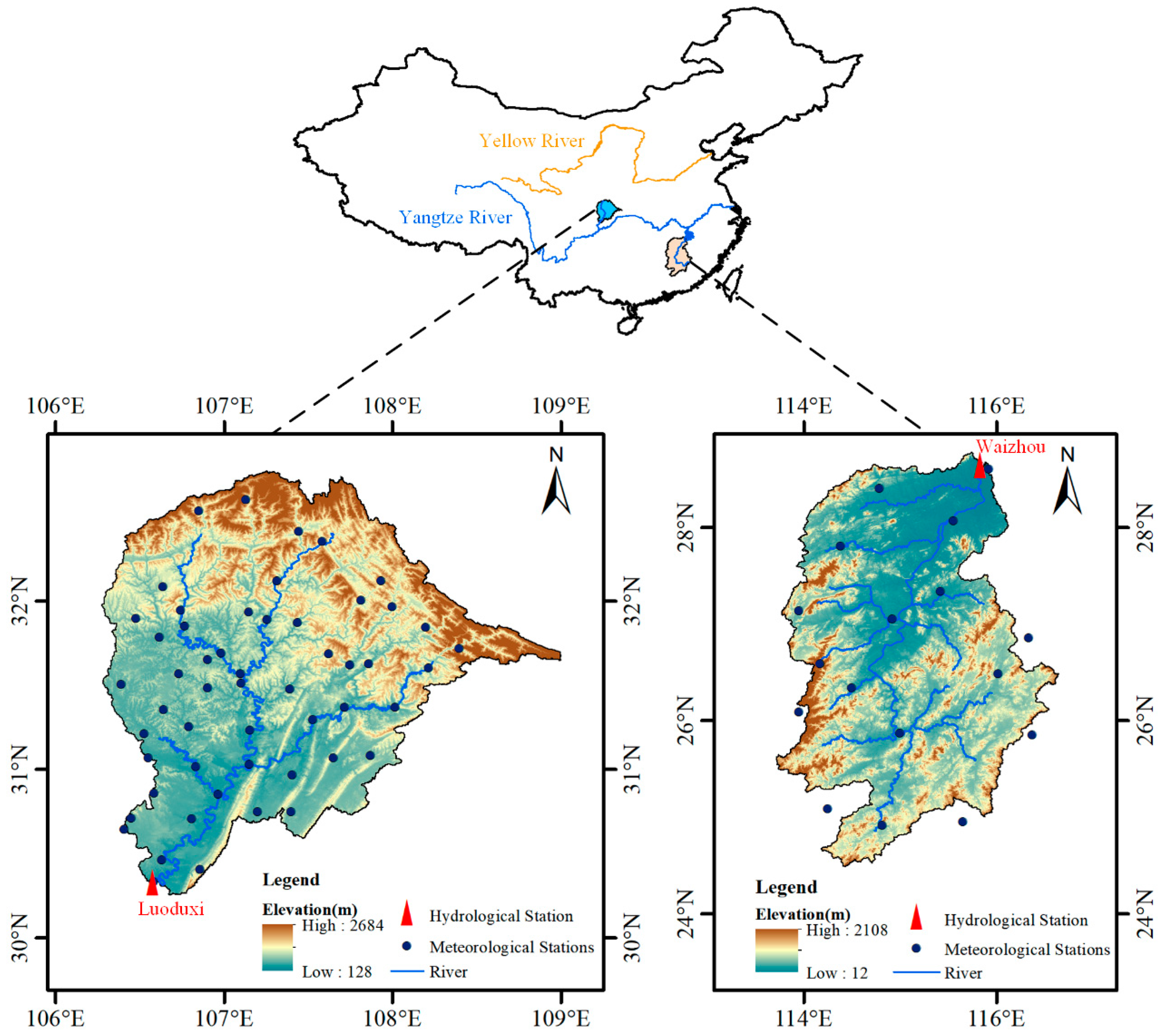
The Qujiang catchment (QJ) and the Ganjiang catchment (GJ) in southern China were chosen as the study area in this study. The location of both QJ and GJ as well as the stations with hydro-meteorological measurements are shown in Figure 1. QJ covers 38,064 km² with Luoduxi station as the catchment outlet and lies between the coordinates 116°10′–119°00′ E and 30°10′–33°00′ N. The elevation within QJ ranges from 128 to 2684 m and decreases from northeast to southwest. GJ is the seventh largest branch of the Yangtze River, located between 113°30′–116°40′ E and 24°29′–29°21′ N, with a drainage area of 81,158 km² above the Waizhou hydrological station. The elevation of GJ ranges from 12 to 2108 m. Both catchments are dominated by a subtropical monsoon climate, with most precipitation and flood events occurring in summer and early autumn. Based on the Digital Elevation Model (DEM) data with a resolution of 1 km, the river channel and watershed boundary for both catchments were delineated using the ArcGIS software (as shown in Figure 1).

2.2. Meteorological Data

The meteorological data required to force DDRM are precipitation P and potential evapotranspiration PET. In this study, daily precipitation and temperature measurements from the period from 1 January 2010 to 31 December 2017 were obtained from 70 (53 for QJ and 17 for GJ) meteorological stations of National Meteorological Information Center of China (http://data.cma.cn/). The daily potential evapotranspiration was calculated using the Blaney-Criddle method [51] from the daily average temperature and the daily sunshine duration. In addition, the daily streamflow data of Luoduxi and Waizhou hydrological station are obtained for the same period as the meteorological data. Daily meteorological data including P and PET of both catchments were then interpolated into the discretized cells (1 km × 1 km) as model inputs using the IDW (Inverse Distance Weighting) method [52].

2.3. SMAP Soil Moisture Product

The SMAP satellite mission is the latest L-band satellite, which aims to retrieve global soil moisture information by measuring brightness temperature through geophysical inversion. The SMAP satellite was launched by NASA on 31 January 2015 and started to provide routine data since 31 March 2015 [28,29,50]. The SMAP mission provides soil moisture products at four different levels, as Level 1 for raw instrument measurements, Level 2 for half orbits based, Level 3 for daily composite, and Level 4 for model assimilation [28]. There currently exists three products of SMAP Level 3 (L3) soil moisture that can be downloaded from National Snow and Ice Data Center (NSIDC, https://nsidc.org/data/smap), including: (1) passive soil moisture product derived from the radiometer signature; (2) active soil moisture product derived from the radar signature; (3) the combined active-passive soil moisture product. The SMAP L3 product is an estimate of surface soil moisture for the top 5 cm of the soil column [25] and covers the period after April 2015. Given the failure of SMAP’s active L-band radar after 2 months in orbit, the passive L-band L3 soil moisture product with a resolution of 9 km (SMAP Enhanced L3 Radiometer Global Daily 9 km EASE-Grid Soil Moisture, Version 2) was chosen for this study.

3. Methodology

3.1. The DEM-Based Distributed Rainfall-Runoff Model (DDRM)

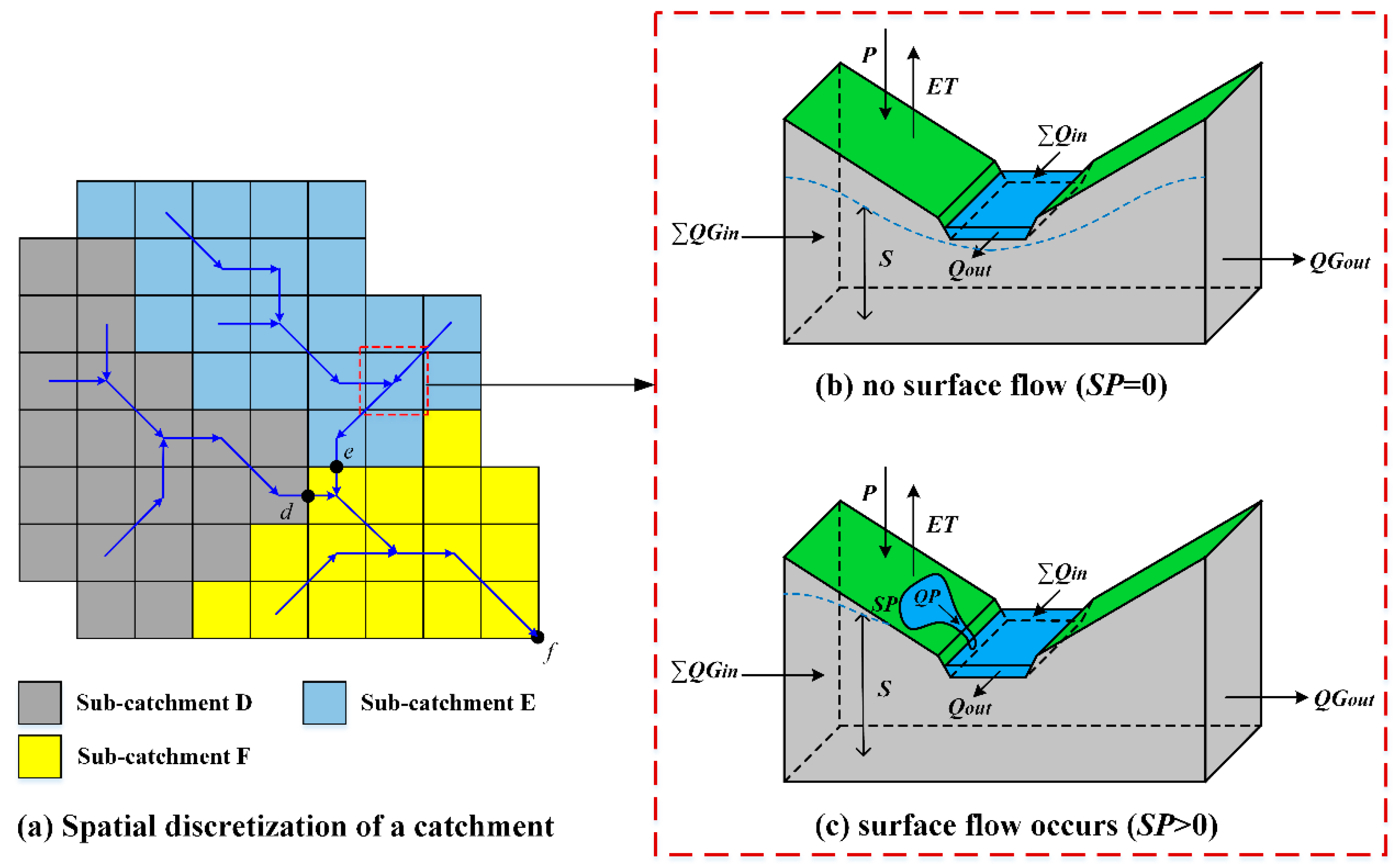
The DEM-based distributed rainfall-runoff model (DDRM) was developed by Xiong et al. [46] and has been tested in several humid and semi-humid catchments of southern China [47,48,49]. To set up DDRM, the study area (catchment) is divided into several sub-catchments which are relatively homogeneous in terms of hydrologic responses; then each sub-catchment is further divided into an array of individual cells, which are treated as the basic hydrologic response units, as demonstrated in Figure 2a. For each cell, three layers are defined to describe the hydrological processes from precipitation to runoff generation and runoff routing, including the river channel layer (blue part in Figure 2b,c), surface layer (green part) and soil layer (grey part).

To account for the spatial heterogeneity of topography and its impact on hydrological process, DDRM assumes that the soil moisture capacity (SMC) of each cell is related to the corresponding topographic index, TI_i. More details about the topographic index can refer to the work of Beven et al. [53]. For cell i, the soil moisture capacity SMC_i is calculated as follows:

$$SM{C}_i=S0+SM·{\left[\frac{T{I}_i-T{I}_{\min }}{T{I}_{\max }-T{I}_{\min }}\right]}^n$$

(1)

where S0 is the minimum water storage capacity and SM stands for the variation range of the water storage capacity across the catchment; n is an empirical constant that reflects the degree of heterogeneity of SMC_i and can take a value between 0 and 1. TI_min and TI_max are the minimum and maximum value of cell-based topographic indexes across the whole catchment, respectively; S0, SM and n are model parameters that require to be calibrated.

DDRM consists of three calculation components: runoff generation at cell scale, sub-catchment outlet streamflow calculation and runoff routing through the river network.

3.1.1. Runoff Generation at Cell Scale

For cell i, the rainfall input for the soil layer at time t is P_i,t. The actual evapotranspiration, ET_i,t, is determined by both potential evapotranspiration PET_i,t and the current water content of the soil layer S_i,t, which is calculated as follows:

$$E{T}_{i,t}=\frac{S_{i,t}}{SM{C}_i}PE{T}_{i,t}$$

(2)

DDRM incorporates the saturation excess runoff mechanism for runoff generation of each cell. Before the soil layer becomes saturated, as shown in Figure 2b, there is no water exchange that occurs between the soil layer and surface layer. When the water content in the soil layer S_i,t exceeds the maximum capacity SMC_i of the cell, as shown in Figure 2c, the excess part S_i,t–SMC_i reaches the surface layer and replenishes the surface ponding water storage SP_i,t, as follows:

$$S{P}_{i,t}=S{P}_{i,t-\Delta t}+S_{i,t}-SM{C}_i$$

(3)

The water content stored in the surface layer turns into surface flow under the force of gravity, and subsequently flows into the river channel layer. The surface flow is calculated under the linear reservoir assumption as:

$$Q{P}_{i,t}=\frac{S{P}_{i,t}}{TP}$$

(4)

where TP is a model parameter that determines the velocity of the surface flow.

For the soil layer, when the water content S_i,t falls below a specific threshold ST_i, the outflow of groundwater is zero. When S_i,t exceeds the threshold ST_i, the groundwater outflow (QSout) is calculated as follows:

$$QSou{t}_{i,t}=\{\begin{array}{ll}\frac{S_{i,t}-S{T}_i}{TS}{(\tan \overline{{\beta }_i})}^b& S_i>S{T}_i\\ 0& S_i<S{T}_i\end{array}$$

(5)

where TS is a model parameter that determines the velocity of the groundwater flow. $\overline{{\beta }_i}$ is the average downward slope across the catchment and b is an empirical constant between 0 and 1. The value of threshold ST_i is smaller than SMC_i and can be calculated by ST_i = α·SMC_i. Here, α is treated as a calibration parameter with a value between 0 and 1.

At time t, the groundwater inflow for cell i can be obtained by:

$$QSi{n}_{i,t}={\displaystyle \sum _{j}QSou{t}_{j,t}}$$

(6)

where QSout_j,t with 0 < j < 8, are the groundwater outflows from the upstream cells of cell i.

At the end of the runoff generation procedure, the water content for the soil layer is updated as below:

$$S_{i,t+\Delta t}=S_{i,t}+\left[P_{i,t}-E{T}_{i,t}\right]·\Delta A·\Delta t+\left[QSi{n}_{i,t}-QSou{t}_{i,t}\right]·\Delta t$$

(7)

where ∆A, ∆t represent the area of each cell and the calculation time step of the model, respectively.

3.1.2. Sub-Catchment Outlet Streamflow Calculation

After the runoff generation calculation for each cell of a certain sub-catchment is completed, the surface flow is routed from upstream cells to downstream cells successively using the Muskingum routing method. The runoff routing procedure begins at the cells that are located at the sub-catchment boundary, then its downstream cells, and ends at the cell with the lowest elevation, i.e., the sub-catchment outlet.

For cell i, the surface inflow for the river channel layer can be obtained by,

$$Qi{n}_{i,t}={\displaystyle \sum _{j}Qou{t}_{j,t}}$$

(8)

where Qout_j,t with 0 < j < 8, are the surface outflows from upstream cells.

The routed surface outflow Qout_i,t is calculated as follows:

$$Qou{t}_{i,t}=c_0\left[Qi{n}_{i,t}+Q{P}_{i,t}\right]+c_1\left[Qi{n}_{i,t-\Delta t}+Q{P}_{i,t-\Delta t}\right]+(1-c_0-c_1)Qou{t}_{i,t-\Delta t}$$

(9)

where c₀ and c₁ are parameters related to the Muskingum routing method at cell scale and take a value between 0 and 1.

3.1.3. Runoff Routing through River Networks

When streamflow simulation for each sub-catchment is completed, the streamflow at the outlet of each sub-catchment (node) is subsequently routed through river networks to downstream nodes. This is also done by applying the Muskingum routing method for each node. As shown in Figure 2a, nodes d and e are the outlets of sub-catchment D and E, respectively. Node f is not only the outlet of sub-catchment F, but also the outlet of the whole catchment. The streamflow at node f (i.e., O_f) consists of three parts: (1) streamflow routed from node d, O_df; (2) streamflow routed from node e, O_ef and (3) local outflow of sub-catchment F, Qout_f, which are calculated as follows:

$$O_{df,t}=h{c}_{0}Qou{t}_{d,t}+h{c}_{1}Qou{t}_{d,t-\Delta t}+(1-h{c}_0-h{c}_1)O_{df,t-\Delta t}$$

(10)

$$O_{ef,t}=h{c}_{0}Qou{t}_{e,t}+h{c}_{1}Qou{t}_{e,t-\Delta t}+(1-h{c}_0-h{c}_1)O_{ef,t-\Delta t}$$

(11)

$$O_{f,t}=O_{df,t}+O_{ef,t}+Qou{t}_{f,t}$$

(12)

where Qout_d and Qout_e represent the runoff of node d and e, respectively; hc₀ and hc₁ are parameters related to the Muskingum routing method at node scale and take a value between 0 and 1.

3.1.4. Model Parameters

As described above, DDRM has 11 parameters, including runoff generation parameters (S0, SM, TS, TP, n, α and b), cell channel routing parameters (c₀ and c₁), and the river networks routing parameters (hc₀ and hc₁). A detailed description of the DDRM parameters are presented in

Table 1. Descriptions of the DEM-based distributed rainfall-runoff mode (DDRM) parameters.

Parameter	Description	Unit	Prior Range
S0	Minimum water storage capacity	mm	1–200
SM	Variation range of water storage capacity across the catchment	mm	1–600
TS	Time constant that determines the velocity of groundwater flow	h	1–300
TP	Time constant that determines the velocity of surface flow	h	1–300
α	Empirical constant describing the characteristic of groundwater flow	-	0–1
b	Empirical constant describing the impact of cell slope on the celerity of groundwater flow	-	0–1
n	Empirical constant describing the relationship between SMC and the corresponding topographic index	-	0–1
c0	Muskingum parameter for runoff routing within a sub-catchment	-	0–1
c1	Muskingum parameter for runoff routing within a sub-catchment	-	0–1
hc0	Muskingum parameter in association with river channel routing	-	0–1
hc1	Muskingum parameter in association with river channel routing	-	0–1

.

3.2. Pre-Processing SMAP Soil Moisture Product

To remove the systematic differences or bias between the raw SMAP soil moisture product and the soil moisture simulated by DDRM, a rescaling procedure is needed. There are several rescaling approaches for this end, including linear rescaling, mean-std rescaling, min-max matching and cumulative distribution function (CDF) matching [15]. Here, the CDF matching method was implemented to rescale the SMAP soil moisture against the DDRM simulated soil moisture (${\theta }^{DDRM}$). This procedure was repeated for each cell within the catchment. As a reference of the CDF matching method, ${\theta }^{DDRM}$ was obtained from the DDRM simulation after a small number of trial parameter calibrations were conducted. Note that the spatial resolution of SMAP L3 soil moisture (9 km) is different from the cell size of DDRM (1 km) in this study. Thus, before the CDF matching procedure, the DDRM simulated soil moisture was resampled into the same spatial resolution with the SMAP data through the nearest resampling technique via ArcGIS platform. Here, the resampled DDRM simulated soil moisture for cell i at time t (i.e., ${\theta }_{i,t}^{DDRM}$) is calculated by:

$${\theta }_{i,t}^{DDRM}=\frac{S_{i,t}·\Delta A}{SM{C}_i·\Delta A}=\frac{S_{i,t}}{SM{C}_i}$$

(13)

Although the CDF matching procedure changes the absolute values of the SMAP soil moisture data, the relative dynamics of the original SMAP is preserved. The rescaled SMAP soil moisture data is denoted by ${\theta }^{CDFM}$ hereafter.

Given that the SMAP soil moisture data only focuses on the top 5 cm of the soil profile, it remains unfeasible to directly compare the rescaled SMAP soil moisture data (i.e., ${\theta }^{CDFM}$) to the DDRM simulated soil moisture (${\theta }^{DDRM}$). This is because the DDRM simulates the dynamic of water content of the whole root-zone. A common solution to this issue is to utilize the exponential filtering technique proposed by Wagner et al. [54] to convert the remote sensing soil moisture data to soil wetness index (SWI) of the root zone. To derive the SWI time series for each cell, the following exponential filter is applied to the ${\theta }^{CDFM}$ series:

$${\theta }_{i,t_n}^{SWI}={\theta }_{i,t_{n-1}}^{SWI}+K_n\left({\theta }_{i,t_n}^{CDMF}-{\theta }_{i,t_{n-1}}^{SWI}\right)$$

(14)

where ${\theta }_{i,t_n}^{SWI}$ is the soil wetness index (SWI) at time t_n for cell i. The gain K at time t_n can be written in recursive form as follows:

$$K_n=\frac{K_{n-1}}{K_{n-1}+e^{-\frac{t_n-t_{n-1}}{T}}}$$

(15)

where the parameter T is a characteristic time length that controls the smoothing degree of the ${\theta }_{i,t_n}^{CDFM}$ series and the response time to the changes in the surface wetness conditions. In this study, T takes the value of 5 days as it provides the best correlation between ${\theta }^{SWI}$ and ${\theta }^{DDRM}$ for both QJ and GJ in a series of trial tests. For the initialization of this filter, K₁ and ${\theta }_{i,t_1}^{SWI}$ were set to 1 and ${\theta }_{i,t_1}^{CDFM}$, respectively.

3.3. Parameter Calibration Schemes

The Kling-Gupta Efficiency (KGE) [55] is used as criteria to access the agreement between the simulated and observed variables, including streamflow and soil moisture series. KGE is calculated as follows:

$$KGE=1-\sqrt{{(r-1)}^2+{({\mu }_s/{\mu }_o-1)}^2+{({\sigma }_s/{\sigma }_o-1)}^2}$$

(16)

where r is the correlation between the simulated and observed variables; μ and σ are the mean and standard deviation of the variables; the subscript s and o represent the simulation and observation data, respectively. KGE value ranges from −∞ to 1, with a value closer to 1 indicating a better simulation performance. To avoid possible ambiguity, KGE_Q is defined to represent the KGE statistic of the simulated streamflow of the watershed outlet, while $KG{E}_{S{M}_i}$ indicates the KGE statistic of the DDRM-simulated soil moisture for cell i,

$$KG{E}_{S{M}_i}=1-\sqrt{{\left(r_{\theta }-1\right)}^2+{\left({\mu }_{{\theta }_i^{DDRM}}/{\mu }_{{\theta }_i^{SWI}}-1\right)}^2+{\left({\sigma }_{{\theta }_i^{DDRM}}/{\sigma }_{{\theta }_i^{SWI}}-1\right)}^2}$$

(17)

where r_θ represents the correlation between ${\theta }_i^{DDRM}$ and ${\theta }_i^{SWI}$; ${\mu }_{{\theta }_i^{DDRW}}$ and ${\mu }_{{\theta }_i^{SWI}}$ are the mean of ${\theta }_i^{DDRM}$ and ${\theta }_i^{SWI}$; ${\sigma }_{{\theta }_i^{DDRM}}$ and ${\sigma }_{{\theta }_i^{SWI}}$ are the standard deviation of ${\theta }_i^{DDRM}$ and ${\theta }_i^{SWI}$, respectively.

In addition, KGE_SM is defined to access the overall simulation performance of soil moisture, as follows:

$$KG{E}_{SM}=\frac{{\displaystyle \sum _{i=1}^{N}KG{E}_{S{M}_i}}}{N}$$

(18)

where N is the number of cells within the whole catchment.

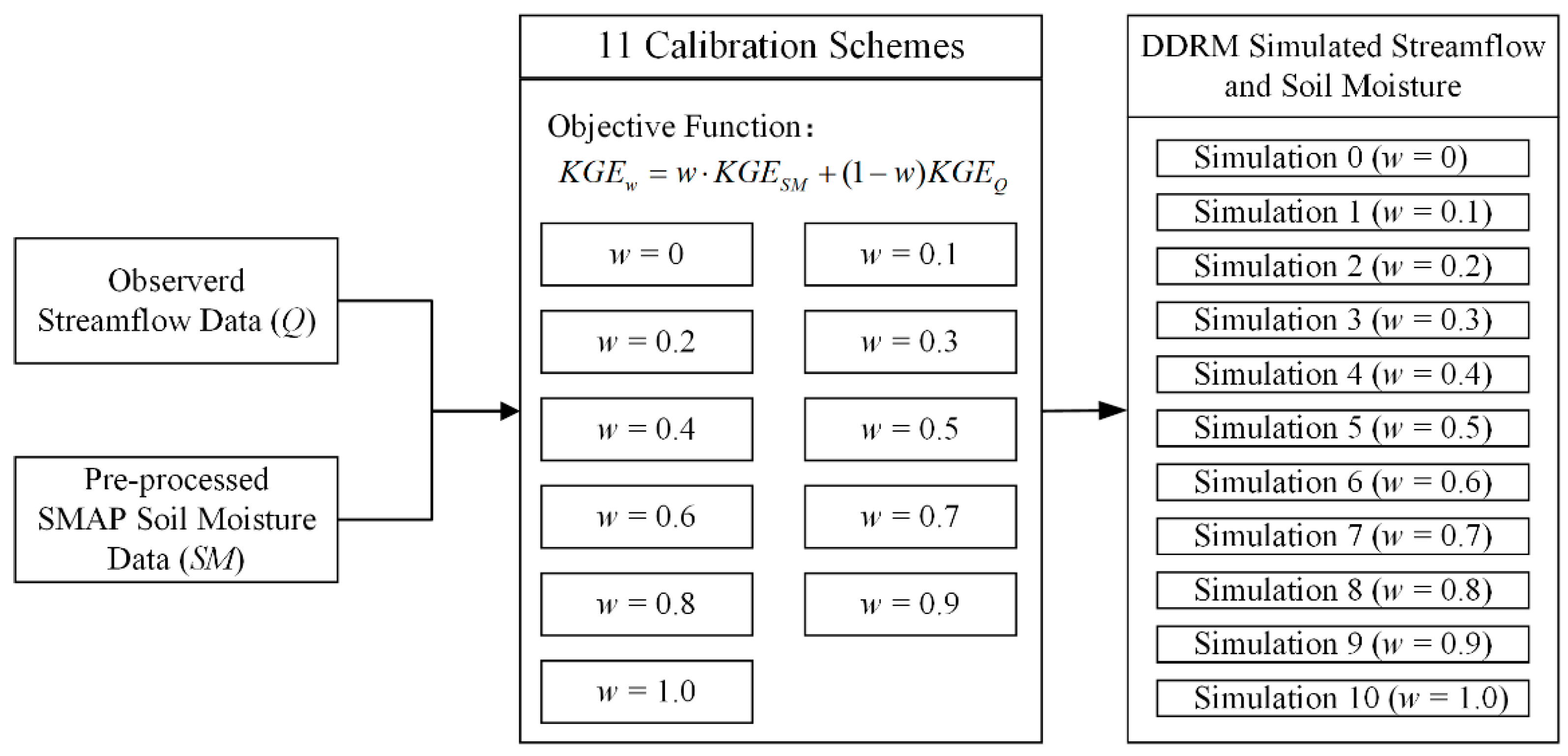
For the parameter calibration purpose, a weighted objective function KGE_w is defined to access the simulation performance in terms of the streamflow of the catchment outlet and the soil moisture, as follows:

$$KG{E}_w=w·KG{E}_{SM}+(1-w)KG{E}_Q$$

(19)

where w is the weight assigned to soil moisture and varies between 0 and 1.

To evaluate the relative effect of remote sensing soil moisture estimates in model calibration, DDRM was calibrated under 11 different schemes for both study catchments. Under the 11 calibration schemes, the w value in the objective function KGE_w was set to 0, 0.1, 0.2, 0.3, 0.4, 0.5, 0.6, 0.7, 0.8, 0.9 and 1.0, respectively (as shown in Figure 3). Note that when w is set to 0, the model is calibrated against only the streamflow data, with KGE_w equal to KGE_Q.

Considering that the SMAP L3 soil moisture data is available since the year of 2015, the calibration period for both QJ and GJ is defined as the period 2014–2017, using the year 2014 as the warm-up period. After the parameter calibration procedure, the model is validated during the period 2010–2013. In this study, parameter calibration for DDRM was performed using the shuffled complex evolution method (SCE-UA) [56].

4. Results and Discussion

4.1. Simulation Performance of Streamflow and Soil Moisture

Table 2. Simulation performance of streamflow and soil moisture under 11 calibration schemes for QJ and GJ.

Catchment	w	Calibration Period			Validation Period
		KGEQ	KGESM	KGEw	KGEQ
QJ	0	0.885	0.483	0.885	0.796
	0.1	0.884	0.497	0.845	0.802
	0.2	0.883	0.504	0.807	0.806
	0.3	0.881	0.511	0.771	0.810
	0.4	0.878	0.516	0.733	0.813
	0.5	0.876	0.518	0.697	0.816
	0.6	0.871	0.522	0.661	0.819
	0.7	0.866	0.524	0.627	0.821
	0.8	0.864	0.524	0.592	0.821
	0.9	0.853	0.528	0.561	0.822
	1.0	-	0.529	-	-
GJ	0	0.905	0.772	0.905	0.826
	0.1	0.901	0.784	0.889	0.824
	0.2	0.899	0.788	0.877	0.822
	0.3	0.904	0.788	0.869	0.817
	0.4	0.913	0.788	0.863	0.815
	0.5	0.901	0.789	0.845	0.812
	0.6	0.895	0.789	0.831	0.809
	0.7	0.901	0.790	0.823	0.798
	0.8	0.898	0.791	0.812	0.794
	0.9	0.893	0.792	0.802	0.779
	1.0	-	0.792	-	-

Note: the symbol “-” indicates that the calculation of KGE value is not applicable.

presents the simulation performance of streamflow and soil moisture under 11 different calibration schemes. It is evident that the highest KGE value for streamflow (i.e., KGE_Q) could be achieved when the weight w was set to 0, without using remote sensing soil moisture data for parameter calibration in the cases of both catchments. Meanwhile, an acceptable simulation of soil moisture was also achieved, where KGE_SM for QJ and GJ are 0.483 and 0.772, respectively. This is in line with the work of Xiong et al. [23]. With w increasing from 0 to 1.0, DDRM shows a better performance for soil moisture simulation, with a slightly decreased ability in terms of streamflow simulation. For QJ, KGE_Q was 0.885 when the model was calibrated against the observed streamflow only, and slightly decreased to 0.876 under the calibration scheme where w was set to 0.5. The lowest KGE_Q value (0.853) was achieved when w was set to 0.9. In the case of GJ, different calibration schemes led to similar streamflow simulation performance in terms of KGE_Q values, with KGE_Q = 0.905 when w was 0 and KGE_Q = 0.893 when w was set to 0.9. This is in line with the work of Li et al. [7] and Sutanudjaja et al. [39], where they found that the joint calibration using both in-situ streamflow and remote sensing soil moisture slightly degrades the streamflow simulation during the calibration period compared with calibration using streamflow only. This may be partially attributed to the inadequacy of the model structure, as the soil layer within DDRM serves as a conceptual module and may fail to accurately represent the soil profile of the real world. Besides, the uncertainty of model inputs (precipitation and potential evapotranspiration) and the pre-processed SWI series may also contribute to the degradation in streamflow simulation during the calibration period in the case of joint calibration [7,11,39].

In the case where w = 1, DDRM presents the best soil moisture simulation for both QJ and GJ. However, the simulated streamflow is quite unreasonable, and it is hard to access the simulation performance of streamflow. As an intermediate variable of hydrological models, soil moisture is affected by parameters that are related to runoff generation only ($S0$, $SM$, $TS$, $TP$, $\alpha$, $b$, $n$ for DDRM). When calibrated using the remote sensing soil data only, these parameters can be ascertained while the parameters that related to runoff routing ($c_0$, $c_1$, $h{c}_0$, $h{c}_1$ for DDRM) become unregulated [5]. In such a case, KGE_Q may take an unpredictable value, and mostly a negative value, which indicates a poor streamflow simulation.

However, the streamflow simulation performance during the validation period shows a distinct trend with the value of w for QJ, where the KGE_Q value during the validation period increases as the weight w increases from 0 to 0.9, with the highest KGE_Q value achieved when w equals to 0.9. This is in line with the findings of Li et al. [7]. This may indicate that calibration using soil moisture can improve the transferability of DDRM across different periods for QJ. The case for GJ is completely different from QJ. Considering that only 10 parameter sets for each catchment were tested here, a more comprehensive analysis with more parameter sets is required to address this issue. This is not the focus of this study but remains an interesting topic that deserves further research.

Table 3. Optimal parameter values under 11 calibration schemes for QJ and GJ.

Catchment	w	Optimal Parameter Value
		S0	SM	TS	TP	α	b	n	c0	c1	hc0	hc1
QJ	0	144.3	491.7	252.7	28.6	0.66	0.001	0.989	0.993	0.003	0.828	0.091
	0.1	138.8	481.2	254.5	28.4	0.65	0.001	0.977	0.993	0.004	0.804	0.102
	0.2	131.4	482.9	254.1	28.4	0.64	0.001	0.965	0.994	0.003	0.788	0.103
	0.3	120.9	491.4	247.4	28.5	0.63	0.001	0.956	0.993	0.003	0.789	0.102
	0.4	112.3	465.9	246.6	28.4	0.62	0.001	0.899	0.992	0.003	0.830	0.105
	0.5	116.6	472.6	243.8	18.5	0.61	0.001	0.971	0.991	0.004	0.783	0.108
	0.6	107.9	439.1	222.4	19.1	0.61	0.001	0.909	0.989	0.005	0.829	0.105
	0.7	101.0	456.9	206.0	19.8	0.61	0.001	0.913	0.992	0.004	0.759	0.112
	0.8	101.1	497.5	213.7	25.1	0.59	0.001	0.961	0.993	0.003	0.739	0.135
	0.9	89.1	393.4	175.8	23.8	0.61	0.001	0.813	0.987	0.005	0.754	0.142
	1.0	95.7	395.4	172.2	24.3	0.61	0.001	0.842	-	-	-	-
GJ	0	198.8	473.0	231.3	176.5	0.33	0.366	0.838	0.998	0.001	0.970	0.025
	0.1	196.3	499.1	299.3	177.1	0.19	0.286	0.903	0.998	0.001	0.949	0.034
	0.2	199.8	488.5	189.0	183.7	0.22	0.427	0.860	0.998	0.001	0.925	0.031
	0.3	195.7	488.9	293.7	160.2	0.15	0.307	0.840	0.997	0.001	0.949	0.027
	0.4	199.1	497.1	298.6	154.1	0.16	0.323	0.732	0.998	0.001	0.959	0.021
	0.5	198.4	499.5	191.3	186.9	0.39	0.429	0.850	0.998	0.001	0.924	0.041
	0.6	199.5	492.8	177.2	181.3	0.38	0.456	0.890	0.998	0.001	0.930	0.061
	0.7	199.2	485.5	196.3	185.4	0.36	0.425	0.842	0.998	0.001	0.899	0.081
	0.8	199.1	482.4	187.1	191.8	0.21	0.467	0.789	0.998	0.001	0.916	0.027
	0.9	199.8	480.4	185.8	194.3	0.12	0.452	0.857	0.997	0.001	0.931	0.034
	1.0	199.9	478.5	192.7	192.2	0.08	0.437	0.832	-	-	-	-

Note: the symbol “-” indicates that the parameter value is not available.

presents the optimal parameter value under 11 calibration schemes for both QJ and GJ. It should be noted that the parameters related to runoff routing are not available under the calibration scheme $w=1$, as explained above. For QJ, the values of the parameter $\alpha$, $b$, $c_0$ and $c_1$ are quite similar under different calibration schemes, while other parameters vary greatly. While in the case of GJ, the values of parameter $S0$, $SM$, $c_0$ and $c_1$ are consistent among different calibration schemes. For example, the optimal values of parameter $S0$ range from 195.7 to 199.9, which is quite narrow when compared to its priori range (1–200).

4.2. Streamflow Simulation under Different Calibration Schemes

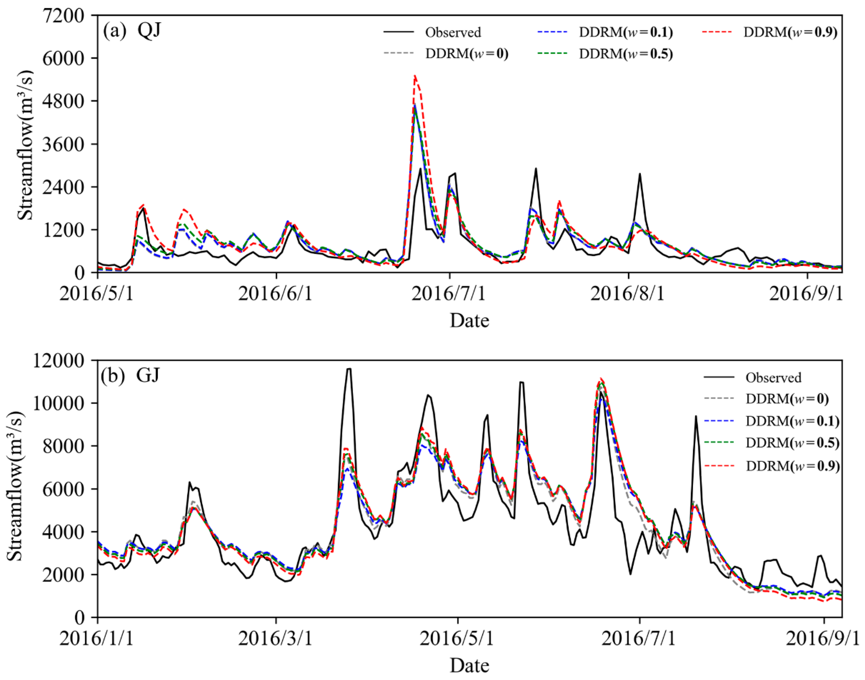
Figure 4 compares the observed streamflow and DDRM simulated streamflow (under four calibration schemes where w = 0, 0.1, 0.5 and 0.9, respectively) for QJ and GJ during part of the calibration period. For the sake of brevity, Figure 4 only covers part of the year 2016. The reason why only the results of the four calibration schemes are presented here is that adjacent values of w lead to pretty similar streamflow simulation performance and may overlap each other. As mentioned in Section 4.1, a lower value of w means a better streamflow simulation performance during the calibration period. In the cases of both QJ and GJ, the DDRM simulated streamflow represented by the red dash line (w = 0.9) tends to overestimate the high flows and underestimate the low flows (exceedance probability 0–10%: high flow; 10–60%, medium flow; 60–100%, low flow), when compared to the blue and green dash line (w = 0.1, 0.5, respectively).

Figure 5 presents the observed flow-duration curve and DDRM simulated flow-duration curves (under 4 calibration schemes where w = 0, 0.1, 0.5 and 0.9, respectively) for QJ and GJ. It can be found that under the calibration scheme where w was set to 0.9, the simulation performance of the high flows and low flows were poor. In contrast, DDRM calibrated using streamflow only (w = 0) shows the best goodness of fit for all flow regimes (low, median and high flows), slightly outperforming those calibrated under other schemes.

Moreover, Figure 6 shows the relative error (RE) between observed and simulated streamflow during the calibration period (2015–2017) under 10 calibration schemes. In the case of QJ, with w increasing from 0 to 0.9, RE for high flow and low flow shows an uptrend while RE for median flow is on a downtrend. The case of GJ is slightly different, where RE for three flow regimes shows no apparent trend as w varies from 0 to 0.9. This is because the streamflow simulation performance under the 10 calibration schemes are very similar, as presented in Table 2.

It can be concluded that incorporating the SMAP soil moisture product into the calibration procedure does not improve the streamflow simulation performance. Furthermore, a greater emphasis on soil moisture (i.e., a larger value of w) during the calibration procedure leads to a slightly worse ability for DDRM to accurately simulate streamflow during the calibration period.

4.3. Soil Moisture Simulation under Different Calibration Schemes

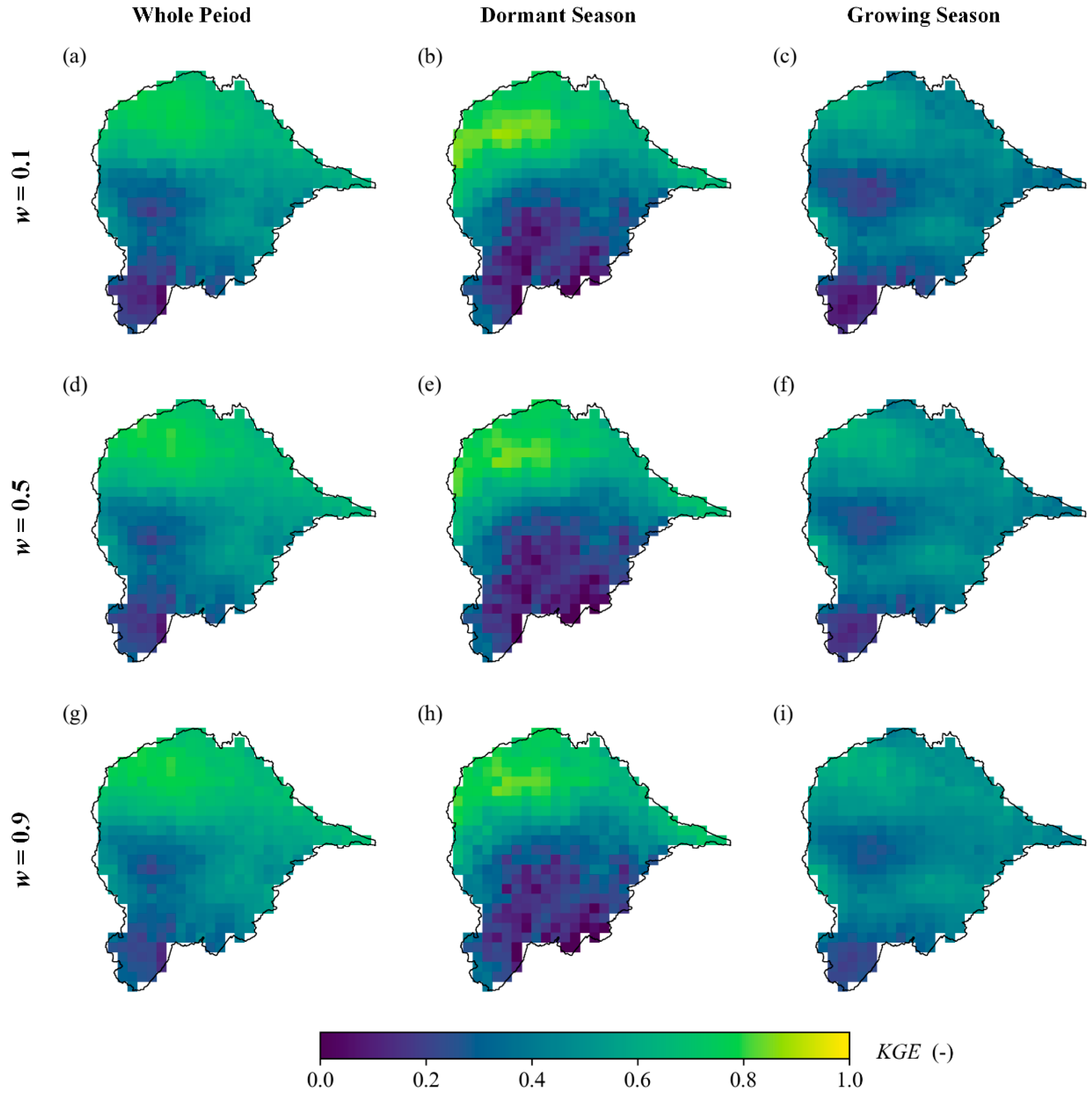
Under 11 calibration schemes, the highest value of KGE_SM was achieved when the weight w was set to 1.0 for both QJ and GJ. Figure 7 and Figure 8 show the spatial distribution of $KG{E}_{S{M}_i}$ values for the whole calibration period, the dormant season (from November to April) and the growing season (from May to October), respectively. For the sake of brevity, only the cases of w = 0.1, 0.5, 0.9 are presented here. It should be noted that very slight difference between the three cases can be detected. This is not unexcepted since the term KGE_SM in the objective function is the average of $KG{E}_{S{M}_i}$ values of all cells within the catchments. For QJ, the spatial distributions of $KG{E}_{S{M}_i}$ values vary between the dormant season and the growing season. During the dormant season, the $KG{E}_{S{M}_i}$ values of northern QJ are much higher than those of southern QJ. In contrast, the spatial distribution of the $KG{E}_{S{M}_i}$ values is quite homogeneous for the growing season. In the case of GJ, the $KG{E}_{S{M}_i}$ values during the growing season are higher than those of the dormant season for most cells within the catchment.

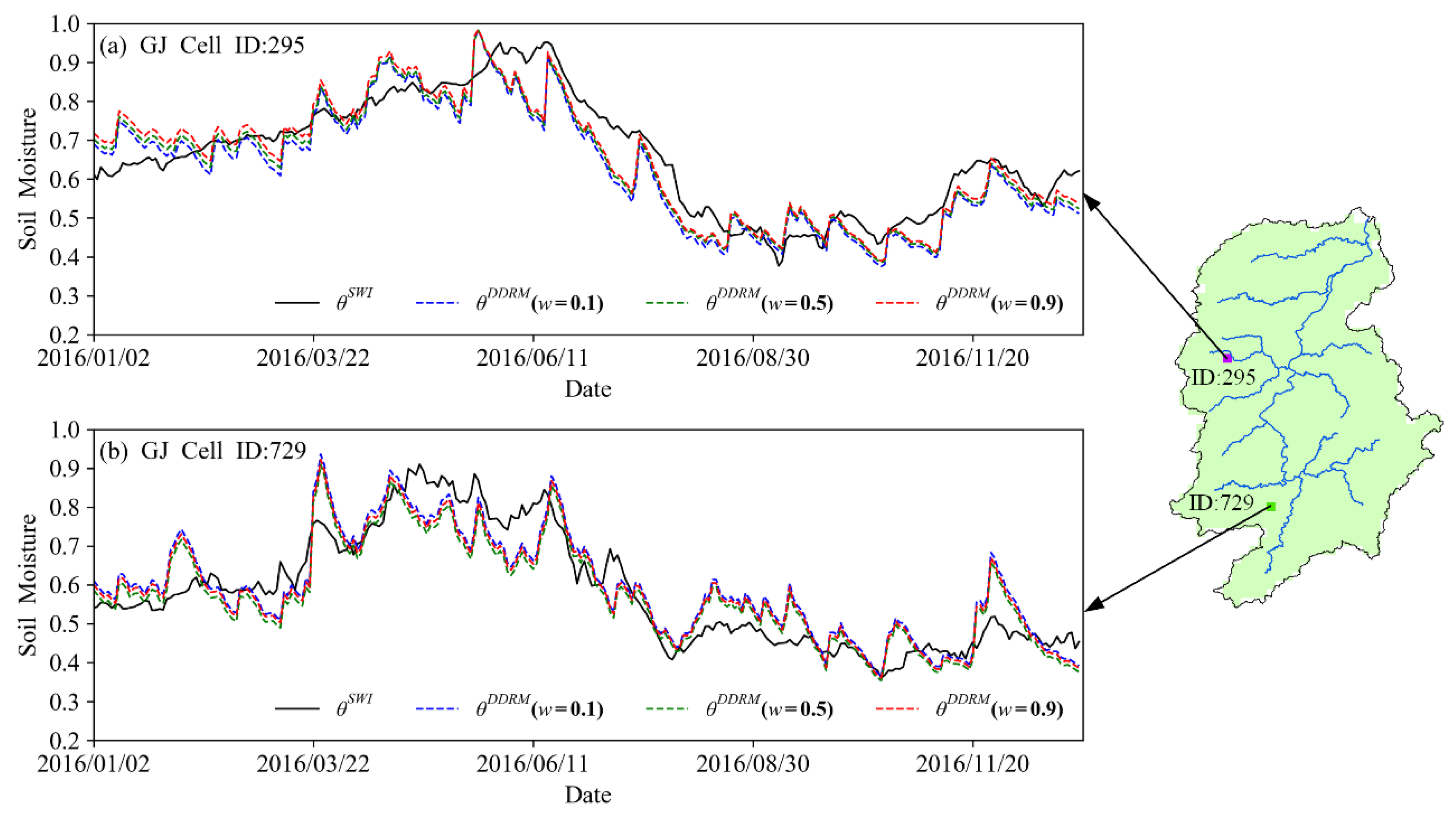
Figure 9 and Figure 10 show the temporal comparison of SWI series ${\theta }_i^{SWI}$ and DDRM simulated soil moisture series ${\theta }_i^{DDRM}$ of two cells for QJ and GJ, respectively. Though the choice of the cells is quite subjective, the cells presented here are representative among all cells within the catchment. Under three calibration schemes (w = 0.1, 0.5, 0.9), the DDRM simulated soil moisture series shows very similar temporal variations. As w increases from 0.1 to 0.9, the DDRM simulated soil moisture series shows a better agreement with the SWI series for these cells.

Though the incorporation of the remote sensing soil moisture data into the calibration procedure fails to achieve a better streamflow simulation, it is an interesting finding that even under the calibration scheme where the weight w was set to 0.1, the DDRM could reproduce an acceptable simulation of the soil moisture series. This indicates that a good simulation of soil moisture does not necessarily collide with a good simulation of streamflow. As a key variable in hydrological models, soil moisture plays a significant role in water content allocation and runoff generation procedures. An accurate simulation of the soil moisture is a prerequisite for reliable streamflow simulating and forecasting.

5. Conclusions

This study incorporated the SMAP soil moisture and streamflow data into the joint calibration of the DEM-based distributed rainfall-runoff model (DDRM) and analyzed the simulation performance of soil moisture and streamflow under 10 different calibration schemes, where the SMAP soil moisture data are assigned to different weights in the objective function. The investigation was carried out for the Qujiang and Ganjiang catchment in southern China. The main findings are as follows:

(1) DDRM can reproduce an acceptable soil moisture simulation when calibrated using the streamflow data only. With a greater emphasis on soil moisture in the joint calibration procedure, the simulation performance of streamflow slightly decreases while a better soil moisture simulation is achieved. However, the difference in simulation performance of these two variables under different calibration schemes is very slight.

(2) From the perspective of flood forecasting, the joint calibration using remote sensing soil moisture and streamflow data shows no apparent advantages in terms of streamflow simulation over the traditional calibration schemes where only streamflow data are used.

It is excepted that a better soil moisture simulation should lead to a better streamflow simulation. However, this is not the case in this study due to the inadequacy of the DDRM model structure and the uncertainty from model inputs (precipitation and potential evapotranspiration) and the remote sensing soil moisture. For the purpose of fully exploring the skill of streamflow prediction, a hydrological model should be calibrated against the historical streamflow data only. For a more realistic representation of the hydrological processes, the joint calibration using both soil moisture and streamflow data can serve as a promising alternative of the traditional calibration approach. Though the compromise between good simulation of soil moisture or streamflow is inevitable for DDRM, this study proves that cost is acceptable as different weights of soil moisture in the objective function cause slight differences in the simulation performance of both soil moisture and streamflow.

Considering the availability of the SMAP soil moisture product, the calibration period (2014–2017) for DDRM was quite short, which prevented a further investigation of the proposed calibration schemes under different climate conditions (e.g., dry period and wet period). Due to the lack of in-situ soil moisture observation, the DDRM simulated soil moisture was used as reference to rescale the SMAP soil moisture. Further studies could focus on how to rescale the remote sensing soil moisture data where reliable in-situ soil moisture data are unavailable. In addition, a more remote sensing soil moisture product (e.g., AMSR-E and SMOS) can be considered in further studies.

References

- Johnston, R.; Smakhtin, V. Hydrological Modeling of Large river Basins: How Much is Enough? Water Resour. Manag. 2014, 28, 2695–2730. [Google Scholar] [CrossRef] [Green Version]
- Keesstra, S.D.; Temme, A.; Schoorl, J.M.; Visser, S.M. Evaluating the hydrological component of the new catchment-scale sediment delivery model LAPSUS-D. Geomorphology 2014, 212, 97–107. [Google Scholar] [CrossRef]
- Thorstensen, A.; Nguyen, P.; Hsu, K.; Sorooshian, S. Using Densely Distributed Soil Moisture Observations for Calibration of a Hydrologic Model. J. Hydrometeorol. 2016, 17, 571–590. [Google Scholar] [CrossRef]
- Beven, K. Prophecy, reality and uncertainty in distributed hydrological modelling. Adv. Water Resour. 1993, 16, 41–51. [Google Scholar] [CrossRef]
- Kundu, D.; Vervoort, R.W.; van Ogtrop, F.F. The value of remotely sensed surface soil moisture for model calibration using SWAT. Hydrol. Process. 2017, 31, 2764–2780. [Google Scholar] [CrossRef]
- Kunnath-Poovakka, A.; Ryu, D.; Renzullo, L.J.; George, B. The efficacy of calibrating hydrologic model using remotely sensed evapotranspiration and soil moisture for streamflow prediction. J. Hydrol. 2016, 535, 509–524. [Google Scholar] [CrossRef]
- Li, Y.; Grimaldi, S.; Pauwels, V.R.N.; Walker, J.P. Hydrologic model calibration using remotely sensed soil moisture and discharge measurements: The impact on predictions at gauged and ungauged locations. J. Hydrol. 2018, 557, 897–909. [Google Scholar] [CrossRef]
- Li, Y.; Grimaldi, S.; Walker, J.; Pauwels, V. Application of Remote Sensing Data to Constrain Operational Rainfall-Driven Flood Forecasting: A Review. Remote Sens. 2016, 8, 456. [Google Scholar] [CrossRef]
- Fenicia, F.; Savenije, H.H.G.; Matgen, P.; Pfister, L. A comparison of alternative multiobjective calibration strategies for hydrological modeling. Water Resour. Res. 2007, 43. [Google Scholar] [CrossRef] [Green Version]
- Revilla-Romero, B.; Beck, H.E.; Burek, P.; Salamon, P.; de Roo, A.; Thielen, J. Filling the gaps: Calibrating a rainfall-runoff model using satellite-derived surface water extent. Remote Sens. Environ. 2015, 171, 118–131. [Google Scholar] [CrossRef] [Green Version]
- Lopez Lopez, P.; Sutanudjaja, E.; Schellekens, J.; Sterk, G.; Bierkens, M. Calibration of a large-scale hydrological model using satellite-based soil moisture and evapotranspiration products. Hydrol. Earth Syst. Sci. Discuss. 2017, 21, 3125–3144. [Google Scholar] [CrossRef] [Green Version]
- Laiolo, P.; Gabellani, S.; Campo, L.; Silvestro, F.; Delogu, F.; Rudari, R.; Pulvirenti, L.; Boni, G.; Fascetti, F.; Pierdicca, N.; et al. Impact of different satellite soil moisture products on the predictions of a continuous distributed hydrological model. Int. J. Appl. Earth Obs. Geoinf. 2016, 48, 131–145. [Google Scholar] [CrossRef]
- Lian, J.; Li, D.; Huang, M.; Chen, H. Evaluation of remote sensing-based evapotranspiration estimates using a water transfer numerical simulation under different vegetation conditions in an arid area. Hydrol. Process. 2018, 32, 1801–1813. [Google Scholar] [CrossRef]
- Zink, M.; Mai, J.; Cuntz, M.; Samaniego, L. Conditioning a Hydrologic Model Using Patterns of Remotely Sensed Land Surface Temperature. Water Resour. Res. 2018, 54, 2976–2998. [Google Scholar] [CrossRef]
- Brocca, L.; Hasenauer, S.; Lacava, T.; Melone, F.; Moramarco, T.; Wagner, W.; Dorigo, W.; Matgen, P.; Martínez-Fernández, J.; Llorens, P.; et al. Soil moisture estimation through ASCAT and AMSR-E sensors: An intercomparison and validation study across Europe. Remote Sens. Environ. 2011, 115, 3390–3408. [Google Scholar] [CrossRef]
- Keesstra, S.; Nunes, J.P.; Saco, P.; Parsons, T.; Poeppl, R.; Masselink, R.; Cerdà, A. The way forward: Can connectivity be useful to design better measuring and modelling schemes for water and sediment dynamics? Sci. Total Environ. 2018, 644, 1557–1572. [Google Scholar] [CrossRef] [PubMed]
- Tianjiao, F.; Wei, W.; Liding, C.; Keesstra, S.D.; Yang, Y. Effects of land preparation and plantings of vegetation on soil moisture in a hilly loess catchment in China. Land Degrad. Dev. 2018, 29, 1427–1441. [Google Scholar] [CrossRef]
- Keesstra, S.D.; Davis, J.; Masselink, R.H.; Casalí, J.; Peeters, E.T.; Dijksma, R. Coupling hysteresis analysis with sediment and hydrological connectivity in three agricultural catchments in Navarre, Spain. J. Soils Sediments 2019, 19, 1598–1612. [Google Scholar] [CrossRef]
- Merz, B.; Plate, E.J. An analysis of the effects of spatial variability of soil and soil moisture on runoff. Water Resour. Res. 1997, 33, 2909–2922. [Google Scholar] [CrossRef] [Green Version]
- Chen, Y.; Yang, K.; Qin, J.; Cui, Q.; Lu, H.; La, Z.; Han, M.; Tang, W. Evaluation of SMAP, SMOS, and AMSR2 soil moisture retrievals against observations from two networks on the Tibetan Plateau. J. Geophys. Res. Atmos 2017, 122, 5780–5792. [Google Scholar] [CrossRef]
- Gebler, S.; Hendricks Franssen, H.J.; Kollet, S.J.; Qu, W.; Vereecken, H. High resolution modelling of soil moisture patterns with TerrSysMP: A comparison with sensor network data. J. Hydrol. 2017, 547, 309–331. [Google Scholar] [CrossRef]
- Gumuzzio, A.; Brocca, L.; Sánchez, N.; González-Zamora, A.; Martínez-Fernández, J. Comparison of SMOS, modelled and in situ long-term soil moisture series in the northwest of Spain. Hydrol. Sci. J. 2016, 61, 2610–2625. [Google Scholar] [CrossRef]
- Xiong, L.; Yang, H.; Zeng, L.; Xu, C. Evaluating Consistency between the Remotely Sensed Soil Moisture and the Hydrological Model-Simulated Soil Moisture in the Qujiang Catchment of China. Water 2018, 10, 291. [Google Scholar] [CrossRef]
- Rötzer, K.; Montzka, C.; Bogena, H.; Wagner, W.; Kerr, Y.H.; Kidd, R.; Vereecken, H. Catchment scale validation of SMOS and ASCAT soil moisture products using hydrological modeling and temporal stability analysis. J. Hydrol. 2014, 519, 934–946. [Google Scholar] [CrossRef]
- O’Neill, P.; Chan, S.; Colliander, A.; Dunbar, S.; Njoku, E.; Bindlish, R.; Chen, F.; Jackson, T.; Burgin, M.; Piepmeier, J.; et al. Evaluation of The Validated Soil Moisture Product from The Smap Radiometerieee. In Proceedings of the 2016 International Symposium on Geoscience and Remote Sensing IGARSS, Beijing, China, 10–15 July 2016; pp. 125–128. [Google Scholar]
- Kerr, Y.H.; Waldteufel, P.; Wigneron, J.; Delwart, S.; Cabot, F.; Boutin, J.; Escorihuela, M.; Font, J.; Reul, N.; Gruhier, C. The SMOS mission: New tool for monitoring key elements ofthe global water cycle. Proc. IEEE 2010, 98, 666–687. [Google Scholar] [CrossRef]
- Lievens, H.; Tomer, S.K.; Al Bitar, A.; De Lannoy, G.J.M.; Drusch, M.; Dumedah, G.; Hendricks Franssen, H.J.; Kerr, Y.H.; Martens, B.; Pan, M.; et al. SMOS soil moisture assimilation for improved hydrologic simulation in the Murray Darling Basin, Australia. Remote Sens. Environ. 2015, 168, 146–162. [Google Scholar] [CrossRef] [Green Version]
- Brown, M.E.; Escobar, V.; Moran, S.; Entekhabi, D.; O’Neill, P.E.; Njoku, E.G.; Doorn, B.; Entin, J.K. NASA’s soil moisture active passive (SMAP) mission and opportunities for applications users. Bull. Am. Meteorol. Soc. 2013, 94, 1125–1128. [Google Scholar] [CrossRef]
- Entekhabi, D.; Njoku, E.G.; O’Neill, P.E.; Kellogg, K.H.; Crow, W.T.; Edelstein, W.N.; Entin, J.K.; Goodman, S.D.; Jackson, T.J.; Johnson, J. The soil moisture active passive (SMAP) mission. Proc. IEEE 2010, 98, 704–716. [Google Scholar] [CrossRef]
- Koster, R.D.; Crow, W.T.; Reichle, R.H.; Mahanama, S.P. Estimating Basin-Scale Water Budgets with SMAP Soil Moisture Data. Water Resour. Res. 2018, 54, 4228–4244. [Google Scholar] [CrossRef]
- Alvarez-Garreton, C.; Ryu, D.; Western, A.W.; Crow, W.T.; Robertson, D.E. The impacts of assimilating satellite soil moisture into a rainfall–runoff model in a semi-arid catchment. J. Hydrol. 2014, 519, 2763–2774. [Google Scholar] [CrossRef]
- Meng, S.; Xie, X.; Liang, S. Assimilation of soil moisture and streamflow observations to improve flood forecasting with considering runoff routing lags. J. Hydrol. 2017, 550, 568–579. [Google Scholar] [CrossRef]
- Sun, L.; Seidou, O.; Nistor, I.; Goïta, K.; Magagi, R. Simultaneous assimilation of in situ soil moisture and streamflow in the SWAT model using the Extended Kalman Filter. J. Hydrol. 2016, 543, 671–685. [Google Scholar] [CrossRef]
- Yan, H.; Moradkhani, H. Combined assimilation of streamflow and satellite soil moisture with the particle filter and geostatistical modeling. Adv. Water Resour. 2016, 94, 364–378. [Google Scholar] [CrossRef]
- Alvarez-Garreton, C.; Ryu, D.; Western, A.W.; Su, C.H.; Crow, W.T.; Robertson, D.E.; Leahy, C. Improving operational flood ensemble prediction by the assimilation of satellite soil moisture: Comparison between lumped and semi-distributed schemes. Hydrol. Earth Syst. Sci. 2015, 19, 1659–1676. [Google Scholar] [CrossRef]
- Leroux, D.J.; Pellarin, T.; Vischel, T.; Cohard, J.; Gascon, T.; Gibon, F.; Mialon, A.; Galle, S.; Peugeot, C.; Seguis, L. Assimilation of SMOS soil moisture into a distributed hydrological model and impacts on the water cycle variables over the Ouémé catchment in Benin. Hydrol. Earth Syst. Sci. 2016, 20, 2827–2840. [Google Scholar] [CrossRef] [Green Version]
- Liu, D.; Mishra, A.K. Performance of AMSR_E soil moisture data assimilation in CLM4.5 model for monitoring hydrologic fluxes at global scale. J. Hydrol. 2017, 547, 67–79. [Google Scholar] [CrossRef]
- Sun, L.; Seidou, O.; Nistor, I.; Liu, K. Review of the Kalman-type hydrological data assimilation. Hydrol. Sci. J. 2016, 61, 2348–2366. [Google Scholar] [CrossRef]
- Sutanudjaja, E.H.; van Beek, L.P.H.; de Jong, S.M.; van Geer, F.C.; Bierkens, M.F.P. Calibrating a large-extent high-resolution coupled groundwater-land surface model using soil moisture and discharge data. Water Resour. Res. 2014, 50, 687–705. [Google Scholar] [CrossRef] [Green Version]
- Rajib, M.A.; Merwade, V.; Yu, Z. Multi-objective calibration of a hydrologic model using spatially distributed remotely sensed/in-situ soil moisture. J. Hydrol. 2016, 536, 192–207. [Google Scholar] [CrossRef] [Green Version]
- Silvestro, F.; Gabellani, S.; Rudari, R.; Delogu, F.; Laiolo, P.; Boni, G. Uncertainty reduction and parameter estimation of a distributed hydrological model with ground and remote-sensing data. Hydrol. Earth Syst. Sci. 2015, 19, 1727–1751. [Google Scholar] [CrossRef] [Green Version]
- Wanders, N.; Bierkens, M.F.P.; de Jong, S.M.; de Roo, A.; Karssenberg, D. The benefits of using remotely sensed soil moisture in parameter identification of large-scale hydrological models. Water Resour. Res. 2014, 50, 6874–6891. [Google Scholar] [CrossRef] [Green Version]
- Wanders, N.; Karssenberg, D.; de Roo, A.; de Jong, S.M.; Bierkens, M.F.P. The suitability of remotely sensed soil moisture for improving operational flood forecasting. Hydrol. Earth Syst. Sci. 2014, 18, 2343–2357. [Google Scholar] [CrossRef] [Green Version]
- Stisen, S.; Koch, J.; Sonnenborg, T.O.; Refsgaard, J.C.; Bircher, S.; Ringgaard, R.; Jensen, K.H. Moving beyond run-off calibration-Multivariable optimization of a surface-subsurface-atmosphere model. Hydrol. Process. 2018, 32, 2654–2668. [Google Scholar] [CrossRef]
- Yassin, F.; Razavi, S.; Wheater, H.; Sapriza-Azuri, G.; Davison, B.; Pietroniro, A. Enhanced identification of a hydrologic model using streamflow and satellite water storage data: A multicriteria sensitivity analysis and optimization approach. Hydrol. Process. 2017, 31, 3320–3333. [Google Scholar] [CrossRef]
- Xiong, L.; Guo, S.; Tian, X. DEM-based distributed hydrological model and its application. Adv. Water Sci. 2004, 15, 517–520. (In Chinese) [Google Scholar]
- Xiong, L.; Guo, S. Distributed Watershed Hydrological Model; China Water Power Press: Beijing, China, 2004. (In Chinese) [Google Scholar]
- Long, H.; Xiong, L.; Wan, M. Application of DEM-based distributed hydrological model in Qingjiang river basin. Resour. Environ. Yangtze Basin 2012, 21, 71–78. (In Chinese) [Google Scholar]
- Zeng, L.; Xiong, L.; Yang, H. Comparison of Soil Moisture Sensed Remotely and Simulated by Hydrological Model in the Xijiang Basin. J. Water Resour. Res. 2018, 7, 339–350. (In Chinese) [Google Scholar]
- Entekhabi, D.; Das, N.; Njoku, E.G.; Jackson, T.J.; Shi, J.C. SMAP L3 Radar/Radiometer Global Daily 9 km EASE-Grid Soil Moisture; National Snow and Ice Data Center: Boulder, CO, USA, 2015. [Google Scholar]
- Blaney, H.F.; Criddle, W.D. Determining Consumptive Use and Irrigation Water Requirements; US Department of Agriculture: Washington, DC, USA, 1962.
- Bartier, P.M.; Keller, C.P. Multivariate interpolation to incorporate thematic surface data using inverse distance weighting (IDW). Comput. Geosci. 1996, 22, 795–799. [Google Scholar] [CrossRef]
- Beven, K.J.; Kirkby, M.J. A physically based, variable contributing area model of basin hydrology. Hydrol. Sci. J. 1979, 24, 43–69. [Google Scholar] [CrossRef]
- Wagner, W.; Lemoine, G.; Rott, H. A Method for Estimating Soil Moisture from ERS Scatterometer and Soil Data. Remote Sens. Environ. 1999, 70, 191–207. [Google Scholar] [CrossRef]
- Gupta, H.V.; Kling, H.; Yilmaz, K.K.; Martinez, G.F. Decomposition of the mean squared error and NSE performance criteria: Implications for improving hydrological modelling. J. Hydrol. 2009, 377, 80–91. [Google Scholar] [CrossRef] [Green Version]
- Duan, Q.; Sorooshian, S.; Gupta, V. Effective and efficient global optimization for conceptual rainfall-runoff models. Water Resour. Res. 1992, 28, 1015–1031. [Google Scholar] [CrossRef]
Figure 1.
Location of the Qujiang basin (QJ) and the Ganjiang basin (GJ) and their corresponding meteorological stations (blue dots) and hydrological station (red triangle).
Figure 2.
The spatial discretization strategy and water balance components for a basic hydrological response unit (cell) within DEM-based distributed rainfall-runoff model (DDRM): (a) discretization of a catchment into sub-catchments and cells; (b) situation where the cell is not saturated, and no surface flow occurs; (c) situation where the cell is saturated and surface flow occurs.
Figure 3.
Eleven calibration schemes for DDRM using both streamflow and the SMAP soil moisture data.
Figure 4.
Comparison of observed streamflow and DDRM-simulated streamflow under four calibration schemes (w = 0, w = 0.1, w = 0.5, w = 0.9) for (a) QJ and (b) GJ.
Figure 5.
Comparison of the observed and DDRM-simulated flow-duration curve during the calibration period (2015–2017) for (a) QJ and (b) GJ.
Figure 6.
Relative Error (RE) in simulated streamflow for (a) QJ and (b) GJ during the calibration period (2015–2017) for three different flow regimes: (Exceedance probability 0–10%: high flow; 10–60%, medium flow; 60–100%, low flow). RE = Abs (Simulated-Observed)/Observed × 100%.
Figure 7.
KGE value between cell-based SWI series () and DDRM-simulated soil moisture series () during the whole period (the left column), the dormant seasons (the middle column) and the growing seasons (the right column) under three calibration schemes (w = 0.1, w = 0.5, w = 0.9, respectively).
Figure 8.
Figure 9.
Temporal comparison of cell-based SWI series () and DDRM-simulated soil moisture series () for QJ. Two cells (a) cell ID 43 and (b) cell ID 280 are shown here for illustration purposes.
Figure 10.
Temporal comparison of cell-based SWI series () and DDRM-simulated soil moisture series () for GJ. Two cells (a) cell ID 295 and (b) cell ID 729 are shown here for illustration purposes.