Laboratory Study of Secondary Flow in an Open Channel Bend by Using PIV


1
State Key Laboratory of Hydroscience and Engineering, Tsinghua University, Beijing 100084, China
2
State Key Laboratory of Hydrology, Water Resources and Hydraulic Engineering, Nanjing Hydraulic Research Institute, Nanjing 210029, China
*
Author to whom correspondence should be addressed.
Water 2019, 11(4), 659; https://doi.org/10.3390/w11040659
Submission received: 7 March 2019
/
Revised: 27 March 2019
/
Accepted: 28 March 2019
/
Published: 30 March 2019
(This article belongs to the Special Issue Advances in Hydraulics and Hydroinformatics)
Abstract
:The present paper aims to gain deeper insight into the evolution of secondary flows in open channel bend. A U-shaped open channel with long straight inflow/outflow reaches was used for experiments. Efforts were made to precisely specify flow conditions and to achieve high precision measurement of quasi-three-dimensional velocities with a multi-pass, two-dimensional PIV (Particle Image Velocimetry) method. The experimental results show that the flow begins to redistribute before entering the bend and it takes a long distance to re-establish to uniform conditions after exiting the bend. Complex secondary flow patterns were found to be present in the bend, as well as in the straight inflow and outflow reaches. A “self-breaking” (process was identified, which correlates stream-wise velocity with the intensity of flow circulation.
1. Introduction
Complex flow patterns exist in open channel bends and they play important roles in alluvial and ecological processes. Curvature-induced secondary flows, for instance, occur as an intrinsic balance between the centrifugal force and the pressure gradient due to water surface tilting. These secondary flows act to redistribute bulk velocity, alter sediment transport, shape bar-pool topography, enhance mass mixing, increase energy loss, and reduce conveyance capacity of the channel [1,2,3,4,5,6,7,8,9,10].
There have been abundant experimental studies on secondary flow in open channel bends. In particular, two important issues were repeatedly addressed: the strength of the secondary flow [11,12,13,14,15] and the interaction between the secondary flow pattern and the main flow [11,16,17,18,19].
Miao et al. [12] reported that, depending on the bend curvature, the normalized magnitude of the secondary flow grows linearly or un-linearly with the ratio of flow depth over bend radius. The Reynolds number was found to play an important role in shaping the secondary flow [11], and the maximum secondary flow strength occurred at the second half of the bend [13]. Roca et al. [14] observed that the maximum vorticity increases along a curved channel from the bend entry until the cross-sections from 40° to 60°. Ramamurthy et al. [15] found that bends with vanes exhibit a lower intensity of secondary flow.
Experiments on the interaction between main flow and secondary flow show that the transverse transport of main flow momentum by the secondary circulation is the principal cause of velocity redistribution, and the deflection of the maximum velocity toward the outer wall of the channel occurs at the cross-section where the secondary flow reaches its maximum strength [11,16,17,18,20]. Particularly, two parameters for the total additional secondary flow term have been defined and examined for their impact on velocity distributions [17].
An extensive literature review also reveals the lack of a reliable quantitative description of the secondary flow along the entire channel. The insufficiency of previous experimental studies can be attributed to three aspects.
Firstly, the limitation in instrumentation hinders precise measurement in some important flow areas. For instance, experiments with ADV/ADVP (Acoustic Doppler Velocity/Acoustic Doppler Velocity Profiler) fail to sample the near-surface and near-bed flow regions [6,13], making it difficult, if not impossible, to explore the number and position of secondary flow cells at each cross-section [17,21]. Other instruments, e.g., velocity meter PROPLER [20] and P-EMS velocimeter [18], are unable to provide three components of a velocity vector. The popularization of PIV (Particle Image Velocimetry) in fluid mechanics shows promise as being a better instrumentation for measurement of curved flows [22,23,24,25,26]. In particular, some novel multi-pass window deformation approaches have been used to improve the performance of PIV in measurement of various flows [27,28,29].
Secondly, the experimental design in most curved flow studies is insufficient for a closer observation of the evolution of the flow along the entire channel, including the bend and the straight inflow/outflow reaches. Some experiments either examined merely one cross-section [4,17,30] or used too long a distance between cross-sections to track the evolution of secondary patterns [11]. In the studies by Blanckaert [31], Vaghefi et al. [13], Abhari et al. [18], Bai et al. [11], Zeng et al. [32], and Booij [30], velocity measurements did not cover the straight inflow or outflow reaches at all.
Thirdly, the influence of the straight inflow/outflow reaches on the secondary flow receives little attention. The inflow/outflow reaches are often short, e.g., only 2 m long compared with a 3.77 m bend in the study by Bai et al. [11]. The curved flume used by Blanckaert [33] has no straight outflow reach at all. The influence of the inflow/outflow reaches still remains unclear, and as a result, the evolution of secondary flow in the bend involves much ambiguity. Some quantitative guidelines obtained by previous studies introduced too many assumptions [12].
To further investigate the evolution of secondary flow in open channel bend, a U-shaped bend with long straight inflow/outflow reaches has been designed and experiments have been conducted. In particular, the paper aims to illustrate the characteristics of the secondary flow at simple but precisely specified conditions to avoid possible ambiguity.
The paper has the following objectives:
- (1)
- To set up a well-designed experimental system that facilitates accurate specification of flow conditions and detailed observation of the three components of flow velocity in a U-shaped open channel flume with long straight inflow/outflow reaches. The experimental design effectively eliminates ambiguity in both the inflow and the outflow reaches and enhances measurement reliability.
- (2)
- To report and interpret detailed and high-quality data on the secondary flow, with focus on the distribution of the main flow, the topography of water surface, and the evolution of the circulation cells.
- (3)
- To present high-quality data on the secondary flows that may be used for validation and calibration of numerical schemes.
2. Experimental Set-Up and Methods
2.1. U-Shaped Flume
Experiments were conducted to investigate flow properties in a U-shaped flume with a 180° bend. Focus was given to the evolution of secondary flows along the entire channel.
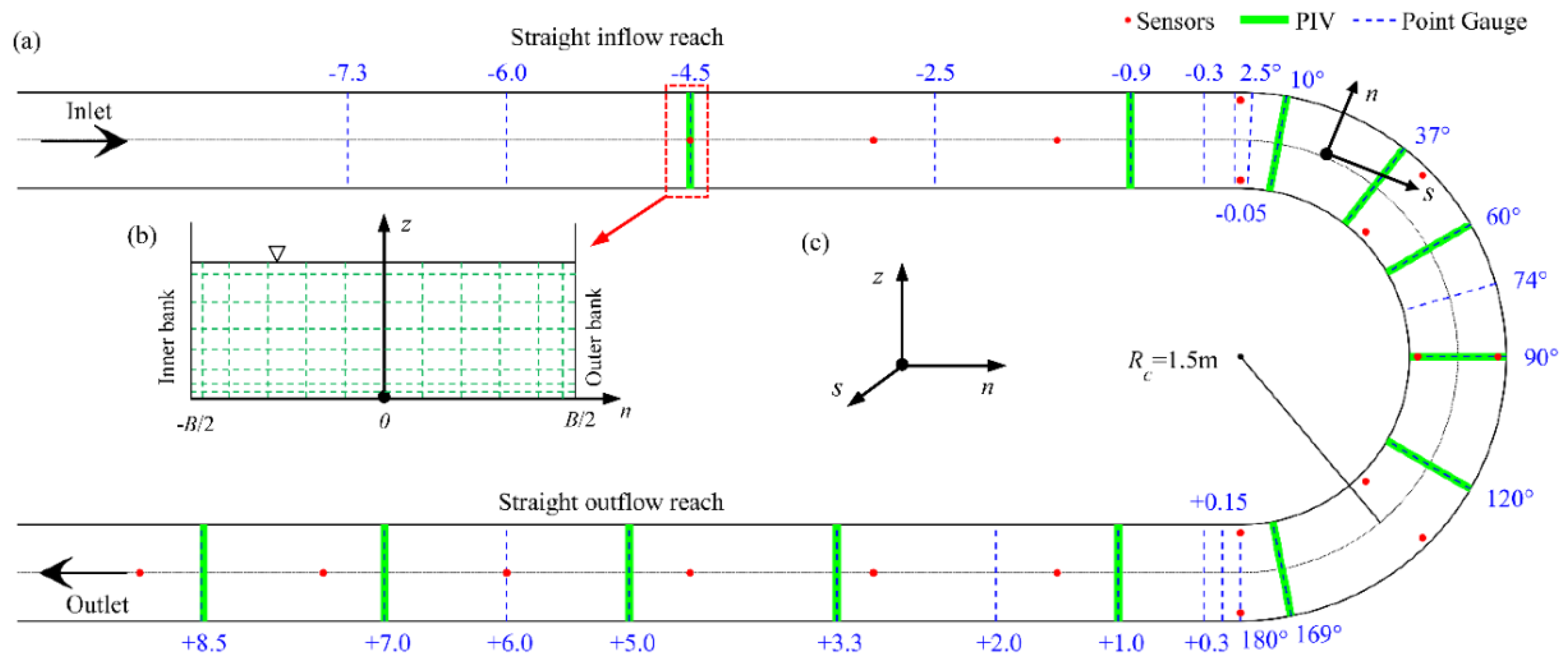
The flume, sketched in Figure 1a, was built with a glass bed and glass side walls. It had a width (B) of 0.3 m, a length along the centerline of approximately 26 m, and a centerline curvature radius (Rc) of 1.5 m. The bend, with a ratio of Rc/B = 5, falls into the category of medium bend [8]. The straight inflow and outflow reaches are both 10 m long, more than twice the length of the bend (center line 4.7 m). A honeycomb was placed at the flume entry to stabilize the flow and attenuate initial large-scale flow structures. A rolling shutter as a tail gate helps to control the water level. The overall stream-wise channel slope is adjustable, but it was fixed at S = 0.001 in the present study.
Figure 1b shows the grids for PIV measurements. Details of the PIV technique will be given later in Figure 2.
The stream-wise, span-wise, and vertical directions are denoted by s, n, and z, respectively (Figure 1c); three components of the time-averaged velocity are U, V, and W.
Flow discharge was measured and controlled by an electromagnetic flow meter. Water surface elevations along the flume were automatically recorded with 20 ultrasonic sensors (red dots in Figure 1a) placed at 15 cross-sections. At each cross-section in the bend (0°, 45°, 90°, 135°, 180°), two sensors were used to monitor the difference in the water level along the span-wise direction. The ultrasonic sensors have a measuring range of 20–200 mm and a measuring error of ±0.2 mm. Real-time monitoring of discharge and water depth facilitates quick stabilization of the flow to steady and uniform conditions. Note that these ultrasonic sensors were used only to monitor the flow rather than to record the water level for further analysis. More precise measurements of water level were achieved with manual point gauge.
2.2. Flow
The flow in the straight inflow/outflow reaches was kept steady and uniform during the experiment. Table 1 shows the hydraulic parameters based on measurements at the cross-section −4.5, 4.5 m upstream of the bend entry. The Reynolds number and Froude number in the straight reaches were 14,917 and 0.557, respectively.
The flow in the experiment is sub-critical, thus the bend plays an important role on the secondary circulation and exerts influence on the inflow by upstream propagation. For sub-critical flows, such influence will diminish.
A water depth of H = 6 cm was used in the experiment, and the corresponding hydraulic radius was R = 4.29 cm. The straight reach of the flume is about 233 R, sufficiently long for the flow to fully develop compared with previous studies by Odgarrd and Bergs [34] and Yen [35], which recommended a straight length of 52 R and 100 R, respectively.
2.3. Measurements
Measurements of water levels and velocity distribution were conducted by means of point gauge and PIV, respectively.
Water surface was measured by manual point gauge with an accuracy of ±0.02 mm at 25 cross-sections (denoted by blue dot lines in Figure 1a) within the entire flume. Information on these 25 cross-sections is given in Table 2. The cross-sections in the straight reaches are denoted by their distance from bend entry (inflow, with minus sign) or from bend exit (outflow, with plus sign), and sections within the bends are denoted by their central angles in degree. For each cross-section, thirteen water depths in the span-wise direction were obtained, and their locations are n = 0, ±3, ±6, ±9, ±12, ±13, and ±14 cm, respectively. Note that the coordinate origin was set at the bottom of the mid-span plane of the channel (see Figure 1a) at each cross section.
A PIV system was employed to measure velocity distributions at 13 cross-sections (green lines in Figure 1a), which are located at the straight inflow reach (−4.5 m and −0.9 m), the bend (10°, 37°, 60°, 90°, 120°, and 169°), and the straight outflow reach (+1.0 m, +3.3 m, +5.0 m, +7.0 m, and +8.5 m).
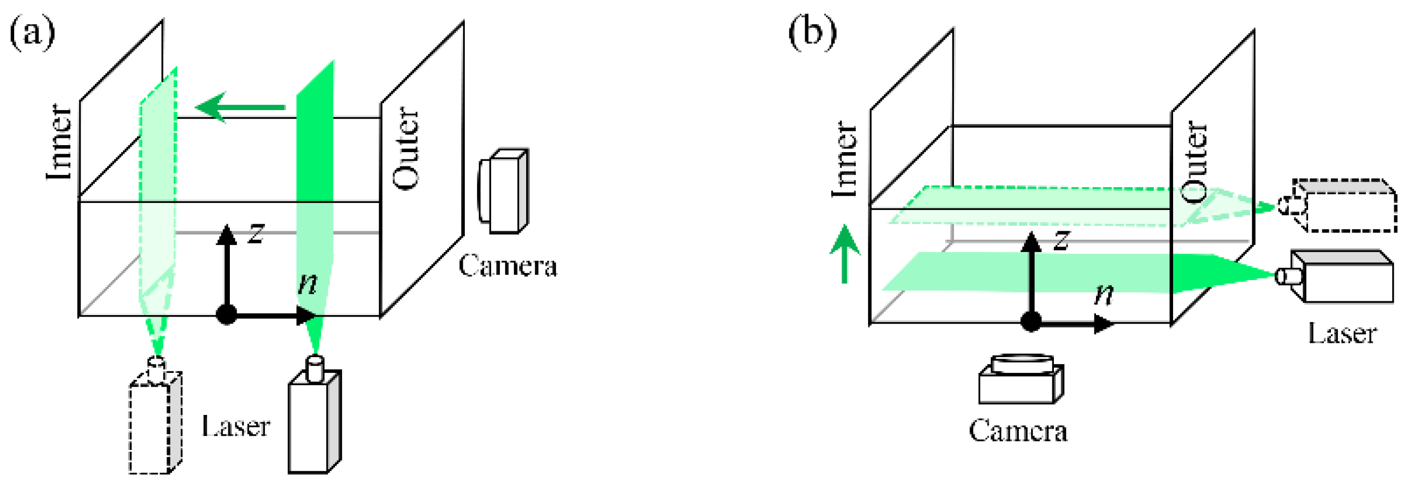
At each cross-section, images in the s-z plane were recorded at eleven span-wise locations, i.e., n = 0, ±3, ±6, ±9, ±12, and ±14 (Figure 1b), to investigate velocity distributions of the stream-wise and vertical components. The image plane, which is normal to the channel bed and parallel to flume wall, is about 8 mm in the stream-wise direction and 6 cm in the vertical direction.
The laser and camera were placed vertically and horizontally, respectively, as shown in Figure 2a. To facilitate operation, a frame was designed with a gear system through which both the laser and the camera can be flexibly adjusted and precisely positioned.
Measurements at the s-n plane were achieved by exchanging the positions of the laser and the camera, as shown in Figure 2b. Images at seven layers were recorded, i.e., z/H = 0.05, 0.1, 0.2, 0.35, 0.5, 0.7, and 0.9, respectively (see Figure 1b). Thus, the stream-wise and span-wise velocity distributions at seven different vertical locations were obtained. A combination of measurements at both s-z and s-n planes provides three-component velocity data in a 11 × 7 grid.
The PIV system uses a continuous wave laser (8 W) at 532 nm for illumination (laser sheet 1 mm thick). The flow was seeded manually with spherical polyamide particles with a density of 1.03 × 10³ kg/m3 and a mean diameter of 5 µm. Particle images were recorded at a frame rate of 500 Hz by an 8-bit 2560 × 1920 pixel high-speed CMOS camera with a Canon EF 50 mm f/1.2 USM lens. Each measurement yields a sample of 15,000 images for analysis, corresponding to a sampling interval of 30 s. The image sizes are 96 pixels × 1120 pixels in Figure 2a, and 2192 pixel × 88 pixel in Figure 2b. Particle images were analyzed using a multi-pass, iterative multi-grid window deformation method. For grid refinement, the following sequence of the interrogation window size in terms of pixel was used: 64 × 64, 32 × 32, and 16 × 16. There is an overlap of 50% in the horizontal direction of the window. Details of the PIV algorithms can be found in Chen et al. [36] and Zhong et al. [37].
As the measurements were conducted in repeated experiments, the repeatability is essential for the validity of the measurements. This was ensured by using a sufficiently large water reservoir to minimize discharge fluctuation, carefully positioning the laser device and camera, and precisely establishing the flow with fixed depth and energy gradient. Comparison of water depth, energy slope, and velocity distribution in the vertical has indicated that the influence of environment change on measurement repeatability was negligible.
2.4. Methods for Data Analysis
2.4.1. Ensemble Average
It is worth noting that the current PIV measurements cannot be used to reconstruct the instantaneous three-dimensional velocity field (or the instantaneous vorticity field) because they refer to different instants. The quasi-3D information of the velocity field is achieved through ensemble average.
For each case, a total number of 15,000 consecutive images were captured at a frame rate of 500 Hz. Previous experience has indicated that such a sample size/interval is sufficient for statistical analysis of mean velocity [36,37]. Based on these instantaneous velocity (u, v, w) samples, the mean velocities (U, V, W) and fluctuating velocity components (u’, v’, w’) were calculated through ensemble average. Examination of the results against the log-law velocity profile and the linear Reynolds stress profile has shown that the data are adequate to evaluate overall properties of the flow.
2.4.2. Data Interpolation
Based on water level measurements at 25 cross-sections, a linear interpolation function has been applied within the bend at an interval of 4.5°.
At each PIV measurement cross-section, based on the three-dimensional velocities at a 7 × 11 grid obtained by matching the s-z plane velocity and s-n plane velocity, an interpolation for the mean velocity has been made to get a final velocity field at a 27 × 57 grid for further analysis.
2.4.3. Calculation of Secondary Flow Strength
Secondary flows at channel bends can be conveniently visualized with velocity vectors and streamlines [13,18,26,38,39]. A more detailed description, however, necessitates the introduction of a quantitative parameter, such as vorticity [4,8,10,13,21,40,41].
The stream-wise component of the instantaneous vorticity vector can be calculated as follows:
where v and w represent instantaneous span-wise and vertical velocity respectively, as defined in Figure 1. Obviously, v = V + v’, where V represents averaged span-wise velocity and v’ represents fluctuating velocity. However, v can be decomposed into a translator part, vn, called instantaneous depth-averaged span-wise velocity, and a circulatory part v*, called the span-wise component of the secondary flow as well as v = vn + v*.
The vorticity provides a good basis for the analysis of transverse circulation.
3. Bulk Flow Distribution
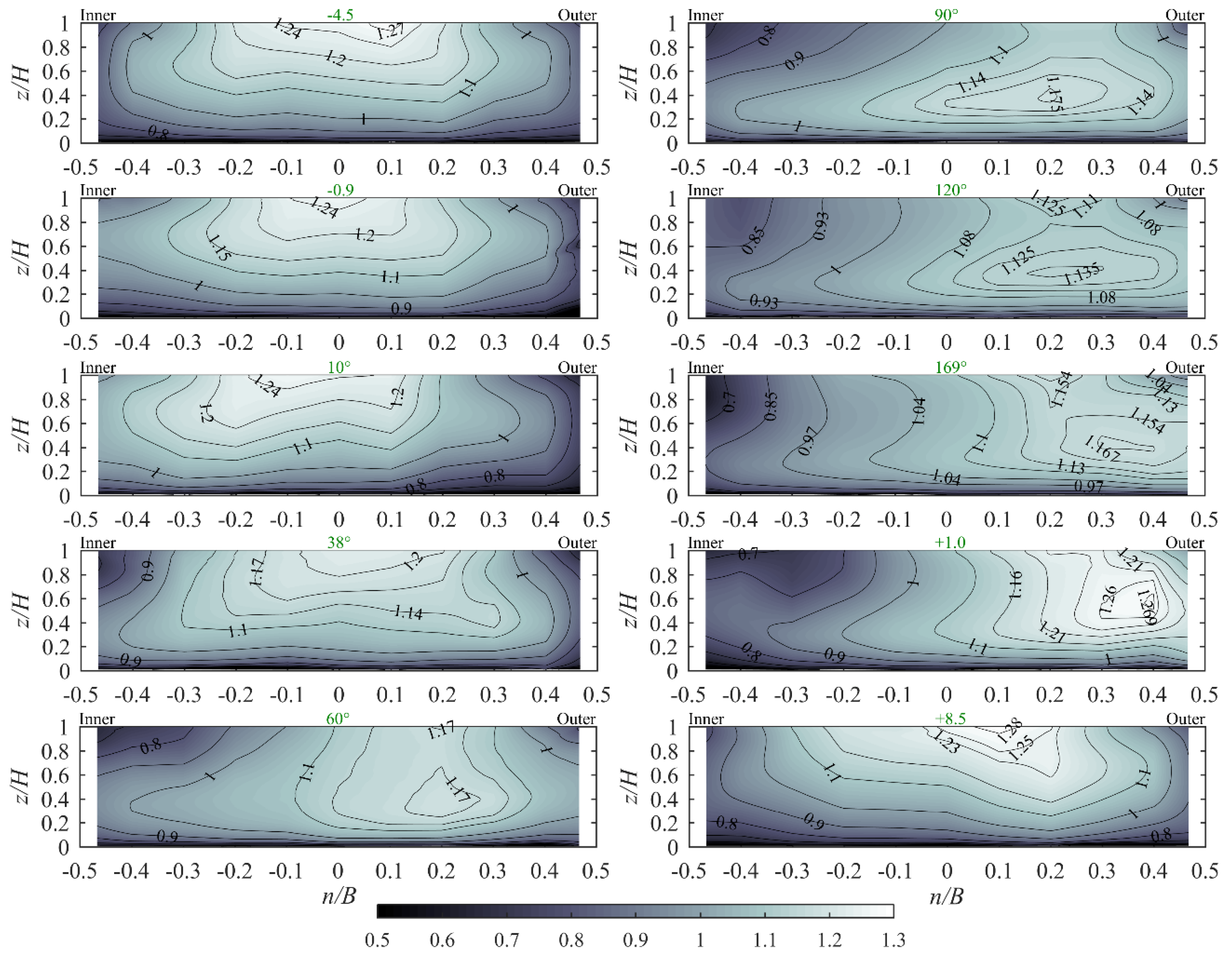
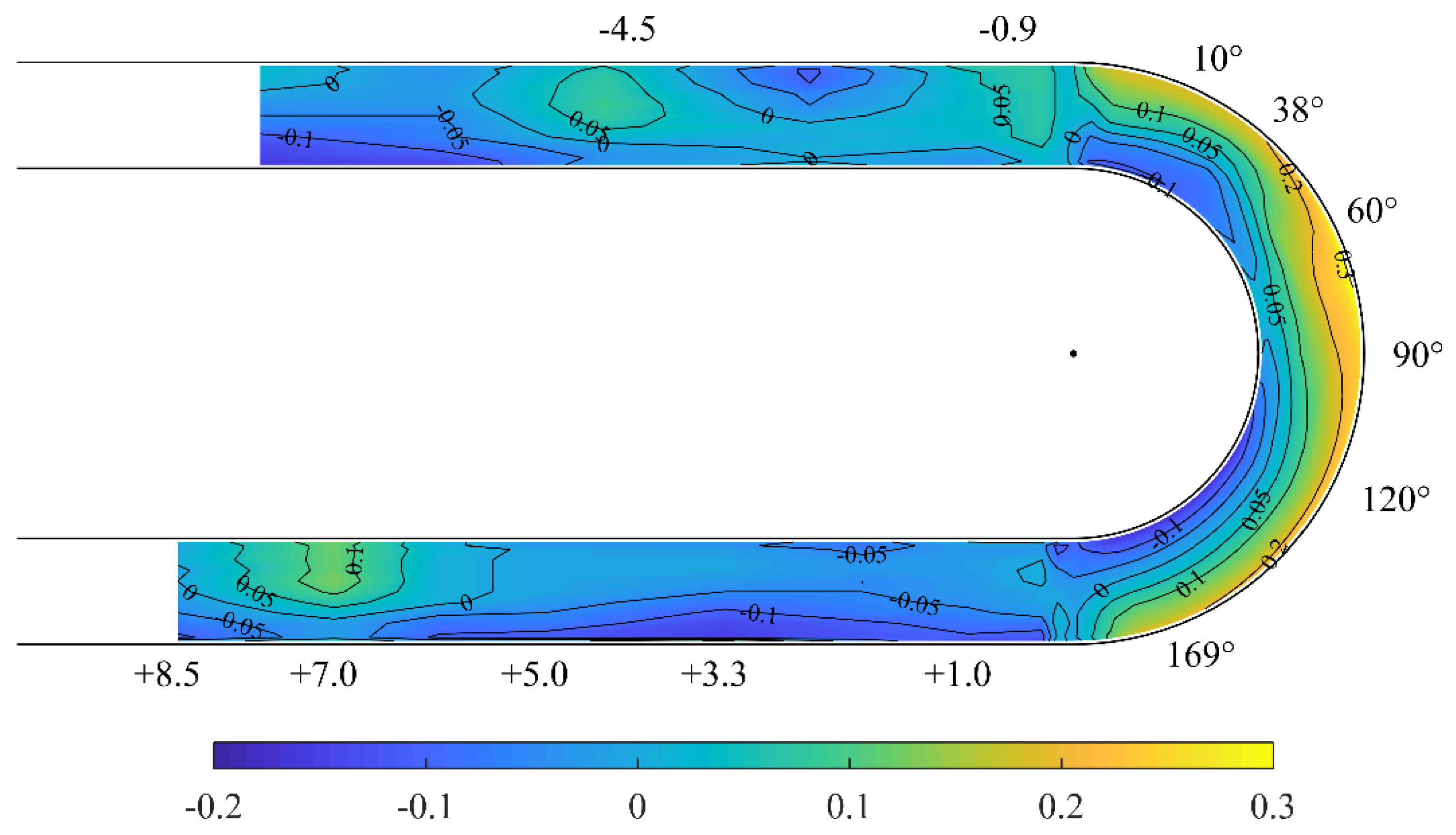
Figure 3 shows contour maps of the vector representations of averaged stream-wise velocity, U, at ten cross-sections. It is obvious that the flow is symmetrical in the straight inflow reach (cross-sections −4.5 and −0.9), deflects to the inner bank in the bend (cross-section 10°) before transferring to the outer bank (cross-sections 60°, 90°, 120°, and 169°), and tends to reconstruct symmetry after exiting the bend in the outflow reach. Note that the flow resumes symmetry at cross-section 38°, a transition cross-section where the main flow achieves balance between the inner and outer banks.
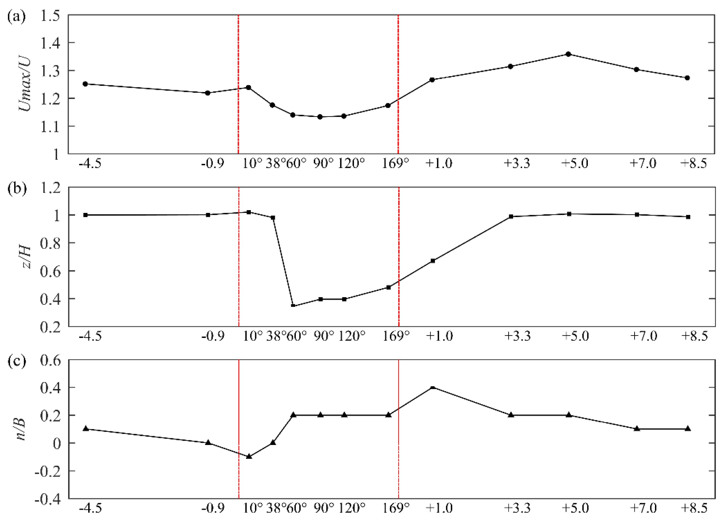
A detailed and quantitative description of the maximum stream-wise velocity, Umax, is given in Figure 4, in terms of both magnitude and position.
The magnitude of Umax, as can be seen in Figure 4a, shows a general decreasing trend when the flow enters the bend, reaches its minimum at cross-section 90°, and then turns to increase in the cross-sections well after the bend. At cross-section +1.0, however, Umax exhibits an unexpected rise over that in the straight inflow reach. This phenomenon may be due to the sudden change of the water level, which creates a positive stream-wise gradient near the outer bank and a negative one near the inner bank.
From the vertical position of Umax in Figure 4b, one can see that the maximum velocity occurs at the water surface in both the straight inflow and outflow reaches. In the channel bend, however, the flow sinks, resulting in a submersion of the maximum velocity well below the water surface. This is particularly noticeable in the central reach of the bend (60°–169°). After the bend, cross-section +1.0 witnesses a rise of water surface followed by a gradual decrease.
The change in the span-wise position of Umax, in Figure 4c, is consistent with established knowledge of curved flows. The flow starts to go toward the inner bank at cross-sections −0.9 and 10°, turns to the outer bank in the rest of the bend, and keeps left-deviated even in the straight outflow reach. It is interesting that the maximum deviation occurs at cross-section +1.0, i.e., 1.0 m away from the bend exit. This indicates that the flow needs a sufficiently long way to re-establish itself to uniform conditions.
To further illustrate the asymmetry of the flow, we introduced another parameter, m, as the horizontal position where the flow discharge is split fifty−fifty. The result is shown in Figure 5. A comparison of Figure 4c and Figure 5 indicates that the change of m in the stream-wise direction is similar to that of n/B, except in the reach from cross-section +3.3 to cross-section +5.0, where the increase of magnitude (Figure 4a) plays a more important role rather than the deflection of position (Figure 5).
Both Figure 4 and Figure 5 reveal that the flow needs a long distance after exiting the bend to re-establish itself, and the curvature has a significant influence not only on the deflection, but also on the magnitude of Umax. For field engineering and numerical simulation of curved flows, such complexity needs in-depth consideration.
4. Secondary Flow Characteristics
4.1. Surface Topography
Based on the measured water depth data from 25 cross-sections, the topography of the water surface in the entire channel was obtained, as shown in Figure 6. Note that the contour represents a subtraction of 6 cm from actual measurement data.
The presence of tilting water surface is a typical feature at channel bends. As expected, a transverse slope was found in the curved flow, i.e., it maintains a negligibly small presence in the straight inflow reach, becomes evident when the flow enters the bend, and reduces to nearly zero immediately after the bend. Within the bend, the outer banks witness a higher transverse slope than the inner bank. The difference in magnitude of transverse slope between the outer and inner banks diminishes in the last third of the bend as the water surface turns to be linear.
The transverse slope depends on a combination of factors, e.g., the incoming flow, the geometry of the bend, and the tail gate. When these factors vary, the transverse slope may display seemingly inconsistent characteristics. For instance, in their experimental and numerical study of a 90° bend with a short exit, Gholami et al. [21] reported a higher degree of surface tilting closer to the inner bank rather than the outer bank, a finding that is contradictory to the present result. In the straight reach of the curved open channel, Blanckaert [7] revealed a significantly larger transverse slope than the present study. Such differences indicate the dependence of flow characteristics on the bend geometry as well as the length of inflow/outflow reaches. If the inflow/outflow characteristics cannot be exactly specified, flow in the bend may exhibit significant variations which hinder verification and calibration of numerical schemes.
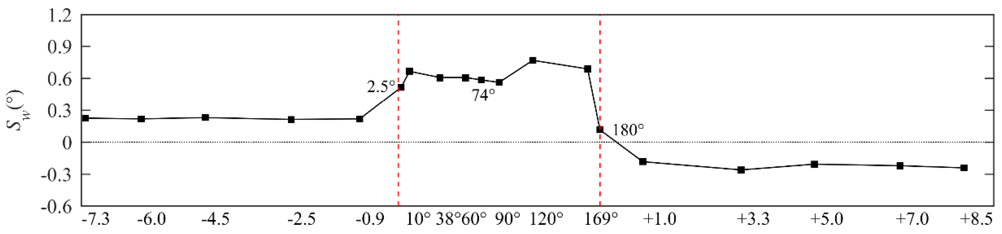
Figure 7 shows the change of the transverse slope along the channel. Note that for each cross-section the transverse slope (in degree) was calculated based on the water depth difference between the outer and inner banks.
In the bend, as we can see, the transverse slope increases quickly and remains at about 0.6 degrees until the end of the bend. At cross-section 120°, the transverse slope reaches its maximum, about 0.8 degrees.
In the straight reaches of the channel, as has been generally acknowledged, the transverse slopes are distinctly smaller. Interestingly, Sw remains positive in the inflow reach and becomes negative in the outflow reach. A positive Sw in the inflow reach is inconsistent with the water tilting in the bend. A negative Sw in the outflow reach is possibly due to the redistribution of flux and transfer of momentum.
4.2. Secondary Flow and Vice Cells
Vice cells of secondary circulation are visible in the experiments. This is critical in the investigation of the number and position of secondary flow.
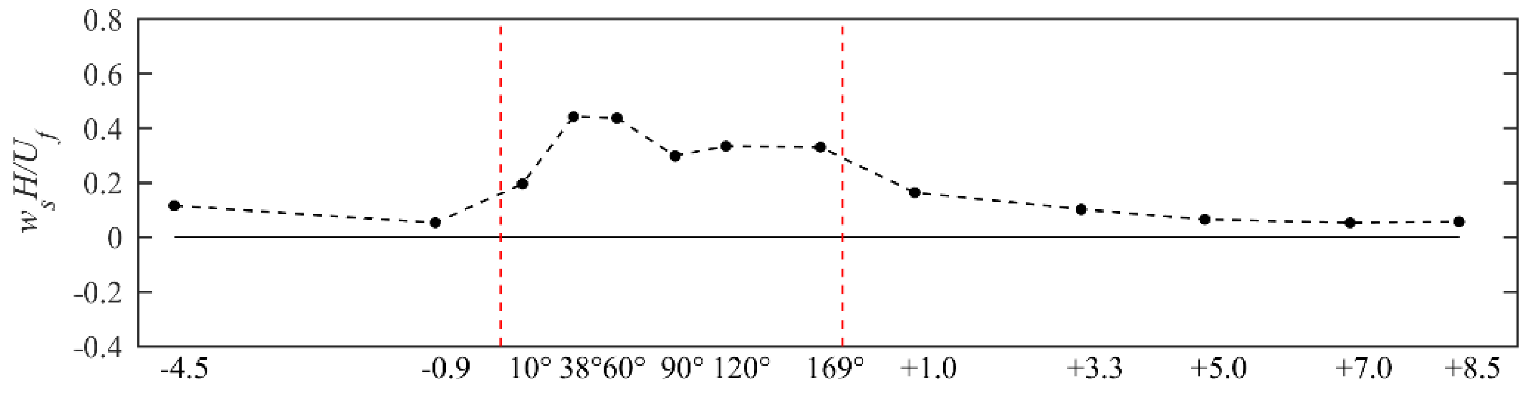
The cross-section-averaged magnitude of vorticity along the flow is shown in Figure 8. Note that the vorticity is normalized by water depth H and cross-section-averaged stream-wise velocity Uf.
In the bend, a gradual increase of transverse circulation is recognized, followed by a decrease. The maximum value occurs at cross-section 60°. The decrease is not distinct after cross-section +3.3. Similar findings have been reported by Rovovikii [42], Blanckaert [31], and Roca et al. [14].
It is interesting that the vorticity reaches its peak at cross-section 60° rather than at 90°, and it keeps roughly constant until 169°. Force analysis below helps to explain this phenomenon.
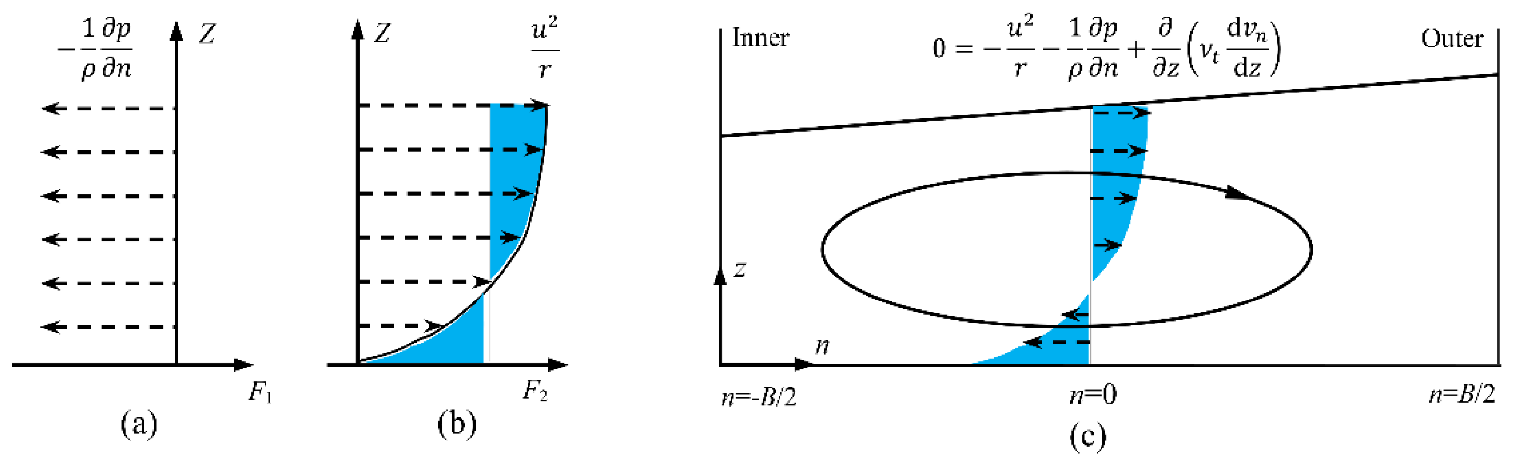
Within a curved channel, secondary circulation occurs as a result of local imbalance between the inward-directed pressure gradient force, −1⁄(ρ∙∂p/∂n), and the outward-directed centrifugal force, u2/r, as shown in Figure 9. The blue areas in Figure 9 represent the local force imbalance which corresponds to the last term in the simplified transverse momentum equation [12].
Obviously, the secondary flow is basically proportional to the local imbalance, which depends on the profile of the stream-wise velocity distribution along the vertical direction and the transverse pressure gradient [4]. The advective momentum transport by the cross-circulation cell brings down the stream-wise velocities in the upper part of the water column and enhances them in the lower part [4,16]. When the stream-wise velocity becomes more evenly distributed along the vertical, the outward centrifugal force will decrease in the upper part and increase in the lower side, as can be seen in Figure 9b. As a result, the intensity of circulation is reduced. There occurs, as it was, a “self-breaking” of circulation.
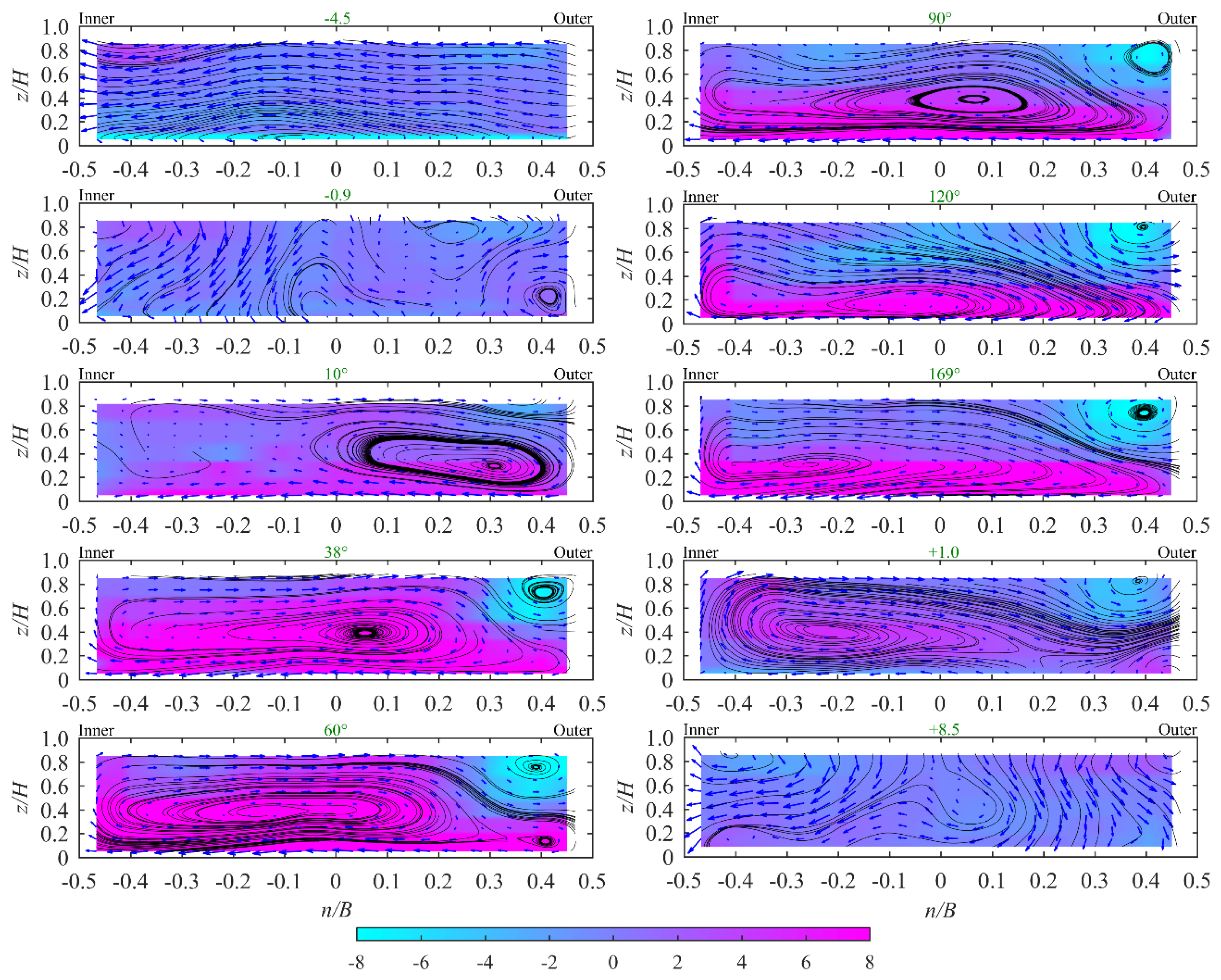
Figure 10 shows the pattern of the stream-wise vorticity and the cross-stream motions in ten cross-sections. The color map represents the vorticity in two senses of rotation, i.e., positive for anticlockwise and negative for clockwise. It is worth noting that the flow takes a relatively long distance for the circulation to decay after exiting the bend.
In cross-section −4.5, one can see that the radial velocity components of the transverse circulation are all oriented to the inner bank. Similar results were also obtained by Gholami et al. [20] and Rozovskii [42]. This one-way radial flow leads to asymmetric velocity distributions, which are consistent with the inner-bank deflection of the stream-wise velocity (Figure 4). Accordingly, the high-velocity zone deviates toward the inner bank at the beginning of the bend.
The changing patterns of the secondary flow are illustrated by the streamlines in Figure 10. As can be seen, circulation appears before the flow enters the bend. The commencement of circulation can be recognized at cross-section −0.9 where the velocity vectors are generally oriented to the inner bank, but a visible circulation cell occurs in the outer-bank region near the bed. This finding is contradictory to the conclusion made by Gholami et al. [20], that no secondary flow exists at the entry of channel bends.
At cross-sections 38°, 60°, 90°, 120°, 169°, and +1.0, a large secondary cell presents across each cross-section and a counter-rotating weaker cell is also identified. These results are consistent with previous findings in both laboratory and field experiments, e.g., Einstein and Harder [43], Rozovskii [42], de Vriend [16], Bridge [44], and Blanckaert et al. [45]. When it rotates, the large secondary cell will transport sediment from the outer bank (where erosion occurs) to the inner bank (where deposition develops) of the bend. The presence of the small counter-rotating cell, in contrast, will attenuate such transportation process and help to protect the bank.
A comparison of cross-sections 10° and 38° reveals a dramatic change in the pattern of the rotating cell. This indicates a fast development of secondary flow in the entry of the bend due to the centrifugal acceleration. At cross-section 10°, the circulation is unique, with a large outer bank cell in the middle of the water depth. This is closely related to the fact that cross-section 10° is the only cross-section whose Umax is close to the inner bank and the core area of the contour (U) deflects to the inner bank (see Figure 3).
A closer look at cross-section 60° shows that near the outer bank, two small circulations occur with different rotation senses, one below the water surface (denoted the third cell) and the other close to the channel bed. This is probably due to the strong dip and deflection of the core of stream-wise velocity (Figure 3 and Figure 4). The mechanism underlying the circulation is complicated by the effect of turbulence anisotropy near the outer bank. Actually, the Umax at cross-section 60° is located near the bed at n/B = 0.3 and z/H = 0.4 (Figure 3), where the big central region separates from the two small outer bank circulation cells.
The third cell occurring at cross-section 60° seems to decay in the following cross-sections and totally disappears at about 90°. This anisotropy generates a stream-wise vorticity of the additional secondary circulation moment, and thus enhances the tendency of the secondary circulation to split up and recur at cross-section +1.0. As the identification of such a small cell requires measurement with high spatial resolution, few previous studies have succeeded in providing detailed information.
The presence of an additional small cell at cross-sections 60° and +1.0 is closely related to the role of the kinetic energy fluxes from turbulence to the mean flow on the generation of the outer bank cell. The results in this paper may help to gain more insight into the kinetic energy transportation.
The outer-bank cell provides a buffer layer that protects the outer bank from any influence of the center-region cell and keeps the core of Umax a certain distance from the bank (Figure 3). At cross-section +1.0, the outer bank cell is very weak, failing to provide a good protection. This phenomenon agrees well with the stream-wise velocity distribution, in that the bulk flow deflects to the outer bank significantly (Figure 4c).
As general knowledge, the outer bank of a bend is more susceptible to erosion. However, the present results, consistent with those of Rovovikii [42], indicate that the most erosion-prone area is the concave bank near the exit from the bend at cross-section +1.0, where a sudden increase in Umax and an attenuation of the counter-rotating cell significantly enhances the erosional force of the flow.
It is surprising that at cross-section +8.5, some weak circulations still exist. This, again, indicates the importance of the length of the straight outflow reach for the flow to re-establish itself.
5. Conclusions
The study reported velocity measurements for the experiments at 25 cross-sections in a U-shaped open channel, based on PIV technique. The PIV system was designed as one which is able to obtain quasi-three-dimensional velocities. The observations focused not only on the bend, but also on the straight inflow/outflow reaches which were designed to be sufficiently long. The velocity distribution, the maximum velocity path, the flow surface topography, and the secondary flow have been evaluated and analyzed. The following conclusions may be drawn:
- (1)
- Streamlines in cross-sections show secondary flows of different patterns along the entire channel. Both the curvature-induced secondary flow and weaker secondary flows, including vice cells, were recognized in the straight inflow/outflow reaches.
- (2)
- The maximum secondary flow occurs at the first half of the bend (cross-section 60°), and a “self-breaking” process was observed, which is consistent with previous studies.
- (3)
- The flow near the entry and exit of the bend is complex due to the sudden change of water surface. Flow redistribution also occurs in the straight inflow and outflow reaches, except the channel bend, indicating that the interaction between the main flow and secondary flow exists along the entire channel. If the inflow/outflow cannot be exactly specified, the flow in the bend may exhibit significant variations.
Author Contributions
R.B. and D.L. conceived and designed the experiments; R.B. collected the data; R.B. and H.C. designed the framework and analyzed the data of this study; D.L. and D.Z provided significant suggestions on the methodology and structure of the manuscript; R.B wrote the paper with the contribution of all co-authors.
Funding
The research was funded by National Key R&D Program of China (2016YFC0402308) and the National Natural Science Foundation of China (Grant no.91647107).
Acknowledgments
The authors are grateful to Wang Xingkui for his help in design of the curved channel.
Conflicts of Interest
The authors declare no conflict of interest.
Abbreviations
| ADV | Acoustic Doppler Velocity |
| ADVP | Acoustic Doppler Velocity Profiler |
| B | channel width (cm) |
| R | hydraulic radius (m) |
| Rc | radius of curvature of channel centerline (m) |
| S | stream-wise channel slope (−) |
| Q | water discharge (m3/s) |
| H | averaged water flow depth along the flume (cm) |
| Uf | cross-averaged stream-wise velocity in the flume (m/s) |
| u* | shear velocity (cm/s) |
| Re | UR/ν is the Reynolds number |
| Re* | u*R/ν is the shear Reynolds number |
| Fr | the Froude number |
| g | gravitational acceleration (ms−2) |
| s | stream-wise reference coordinate (−) |
| n | span-wise reference coordinate; −15 cm represents the inner bank and 15 cm represents the outer one (−) |
| N | sample size (−) |
| z | vertical reference coordinate (−) |
| u | instantaneous stream-wise velocity (m/s) |
| v | instantaneous span-wise velocity (m/s) |
| w | instantaneous vertical velocity (m/s) |
| u’ | instantaneous fluctuating stream-wise velocity (m/s) |
| v’ | instantaneous fluctuating span-wise velocity (m/s) |
| w’ | instantaneous fluctuating vertical velocity (m/s) |
| U | averaged stream-wise velocity (m/s) |
| V | averaged span-wise velocity (m/s) |
| W | averaged vertical velocity (m/s) |
| vn | instantaneous depth-averaged span-wise velocity (m/s) |
| Vn | time-averaged value of vn (m/s) |
| v* | span-wise component of the secondary circulation, v* = v − V (m/s) |
| V* | time averaged value of v* (m/s) |
| Inner | Inner bank (−) |
| Outer | Outer bank (−) |
| θ | cross-section angle (°) |
| ws | stream-wise vorticity, ws = ∂w/∂n − ∂v/∂z (s−1) |
| ρ | density of water (kg/m3) |
| h | local water flow depth (cm) |
| Umax | the highest value of U in a cross-section (m/s) |
| m | the deviation of equipartition position (m) |
| N | sample size (−) |
| P | pressure (Pa) |
| Sw | transverse water surface slope (°) |
References
- Shiono, K.; Muto, Y.; Knight, D.W.; Hyde, A.F.L. Energy losses due to secondary flow and turbulence in meandering channels with overbank flows. J. Hydraul. Res. 1999, 37, 641–664. [Google Scholar] [CrossRef]
- Edwards, B.F.; Smith, D.H. Critical wavelength for river meandering. Phys. Rev. E 2001, 63, 45304. [Google Scholar] [CrossRef] [PubMed]
- Lancaster, S.T.; Bras, R.L. A simple model of river meandering and its comparison to natural channels. Hydrol. Process. 2002, 16, 1–26. [Google Scholar] [CrossRef]
- Blanckaert, K.; Graf, W.H. Momentum Transport in Sharp Open-Channel Bends. J. Hydraul. Eng. 2004, 130, 186–198. [Google Scholar] [CrossRef]
- Sin, K. Methodology for Calculating Shear Stress in a Meandering Channel; Colorado State University: Fort Collins, CO, USA, 2010. [Google Scholar]
- Roca, M.; Martín-Vide, J.P.; Blanckaert, K. Reduction of Bend Scour by an Outer Bank Footing: Footing Design and Bed Topography. J. Hydraul. Eng. 2007, 133, 139–147. [Google Scholar] [CrossRef]
- Blanckaert, K. Flow separation at convex banks in open channels. J. Fluid Mech. 2015, 779, 432–467. [Google Scholar] [CrossRef]
- Kashyap, S.; Constantinescu, G.; Rennie, C.D.; Post, G.; Townsend, R. Influence of Channel Aspect Ratio and Curvature on Flow, Secondary Circulation, and Bed Shear Stress in a Rectangular Channel Bend. J. Hydraul. Eng. 2012, 138, 1045–1059. [Google Scholar] [CrossRef]
- Silva, A.M.F.D.; Yalin, M.S. Fluvial Processes, 2nd ed.; CRC Press/Balkema: London, UK, 2001. [Google Scholar]
- Roca, M.; Martín-Vide, J.P.; Blanckaert, K. Bend scour reduction and flow pattern modification by an outer bank footing. In Proceedings of the International Conference on Fluvial Hydraulic, Lisbon, Portugal, 6–8 September 2012; pp. 1793–1799. [Google Scholar]
- Bai, Y.; Song, X.; Gao, S. Efficient investigation on fully developed flow in a mildly curved 180° open-channel. J. Hydroinform. 2014, 16, 1250–1264. [Google Scholar] [CrossRef]
- Wei, M.; Blanckaert, K.; Heyman, J.; Li, D.; Schleiss, A.J. A parametrical study on secondary flow in sharp open-channel bends: Experiments and theoretical modelling. J. Hydro-Environ. Res. 2016, 13, 1–13. [Google Scholar] [CrossRef]
- Vaghefi, M.; Akbari, M.; Fiouz, A.R. An experimental study of mean and turbulent flow in a 180 degree sharp open channel bend: Secondary flow and bed shear stress. KSCE J. Civ. Eng. 2015, 20, 1582–1593. [Google Scholar] [CrossRef]
- Roca, M.; Blanckaert, K.; Martín-Vide, J.P. Reduction of Bend Scour by an Outer Bank Footing: Flow Field and Turbulence. J. Hydraul. Eng. 2009, 135, 361–368. [Google Scholar] [CrossRef]
- Ramamurthy, A.S.; Han, S.S.; Biron, P.M. Characteristics of Flow around Open Channel 90° Bends with Vanes. J. Irrig. Drain. Eng. 2011, 137, 668–676. [Google Scholar] [Green Version]
- De Vriend, H.J. Velocity redistribution in curved rectangular channels. J. Fluid Mech. 1981, 107, 423. [Google Scholar] [CrossRef]
- Tang, X.; Knight, D.W. The lateral distribution of depth-averaged velocity in a channel flow bend. J. Hydro-Environ. Res. 2015, 9, 532–541. [Google Scholar] [CrossRef]
- Abhari, M.N.; Ghodsian, M.; Vaghefi, M.; Panahpur, N. Experimental and numerical simulation of flow in a 90° bend. Flow Meas. Instrum. 2010, 21, 292–298. [Google Scholar] [CrossRef]
- Termini, D.; Piraino, M. Experimental analysis of cross-sectional flow motion in a large amplitude meandering bend. Earth Surf. Process. Landf. 2011, 36, 244–256. [Google Scholar] [CrossRef]
- Gholami, A.; Akhtari, A.A.; Minatour, Y.; Bonakdari, H.; Javadi, A.A. Experimental and numerical study on velocity fields and water surface profile in a strongly-curved 90° open channel bend. Eng. Appl. Comput. Fluid Mech. 2014, 8, 447–461. [Google Scholar] [CrossRef]
- Farhadi, A.; Sindelar, C.; Tritthart, M.; Glas, M.; Blanckaert, K.; Habersack, H. An investigation on the outer bank cell of secondary flow in channel bends. J. Hydro-Environ. Res. 2018, 18, 1–11. [Google Scholar] [CrossRef]
- Van der Kindere, J.W.; Laskari, A.; Ganapathisubramani, B.; de Kat, R. Pressure from 2D snapshot PIV. Exp. Fluids 2019, 60, 32. [Google Scholar] [CrossRef]
- Scharnowski, S.; Bross, M.; Kähler, C.J. Accurate turbulence level estimations using PIV/PTV. Exp. Fluids 2019, 60, 1. [Google Scholar] [CrossRef]
- Kalpakli Vester, A.; Sattarzadeh, S.S.; Örlü, R. Combined hot-wire and PIV measurements of a swirling turbulent flow at the exit of a 90° pipe bend. J. Vis. 2016, 19, 261–273. [Google Scholar] [CrossRef]
- Nishi, Y.; Sato, G.; Shiohara, D.; Inagaki, T.; Kikuchi, N. A study of the flow field of an axial flow hydraulic turbine with a collection device in an open channel. Renew. Energy 2019, 130, 1036–1048. [Google Scholar] [CrossRef]
- Lindken, R.; Merzkirch, W. A novel PIV technique for measurements in multiphase flows and its application to two-phase bubbly flows. Exp. Fluids 2002, 33, 814–825. [Google Scholar] [CrossRef]
- Termini, D.; Di Leonardo, A. Efficiency of a Digital Particle Image Velocity (DPIV) Method for Monitoring the Surface Velocity of Hyper-Concentrated Flows. Geosciences 2018, 8, 383. [Google Scholar] [CrossRef]
- Sarno, L.; Carleo, L.; Papa, M.N.; Villani, P. Experimental Investigation on the Effects of the Fixed Boundaries in Channelized Dry Granular Flows. Rock Mech. Rock Eng. 2018, 51, 203–225. [Google Scholar] [CrossRef]
- Sarno, L.; Carravetta, A.; Tai, Y.C.; Martino, R.; Papa, M.N.; Kuo, C.Y. Measuring the velocity fields of granular flows—Employment of a multi-pass two-dimensional partical image velocimetry (2D-PIV) approach. Adv. Power Technol. 2018, 29, 3107–3123. [Google Scholar] [CrossRef]
- Booij, R. Measurements and large eddy simulations of the flows in some curved flumes. J. Turbul. 2003, 4, 1–17. [Google Scholar] [CrossRef]
- Blanckaert, K. Flow and Turbulence in Sharp Open-Channel Bends; EPFL: Lausanne, Switzerland, 2002. [Google Scholar]
- Zeng, J.; Constantinescu, G.; Blanckaert, K.; Weber, L. Flow and bathymetry in sharp open-channel bends: Experiments and predictions. Water Resour. Res. 2008, 44. [Google Scholar] [CrossRef] [Green Version]
- Blanckaert, K.; Graf, W.H. Mean flow and turbulence in open-channel bend. J. Hydraul. Eng. 2001, 127, 835–847. [Google Scholar] [CrossRef]
- Odgaard, A.J.; Bergs, M.A. Flow processes in a curved alluvial channel. Water Resour. Res. 1988, 24, 45–56. [Google Scholar] [CrossRef]
- Yen, B.C. On establishing uniform channel flow with tail gate. Proc. Inst. Civ. Eng.-Water Marit. Eng. 2003, 156, 281–283. [Google Scholar] [CrossRef]
- Chen, H.; Zhong, Q.; Wang, X.; Li, D. Reynolds number dependence of flow past a shallow open cavity. Sci. China Technol. Sci. 2014, 57, 2161–2171. [Google Scholar] [CrossRef]
- Zhong, Q.; Li, D.; Chen, Q.; Wang, X. Coherent structures and their interactions in smooth open channel flows. Environ. Fluid Mech. 2015, 15, 653–672. [Google Scholar] [CrossRef]
- Moser, R.D.A.P. Direct Numerical Simulation of Curved Turbulent Channel Flow; National Aeronautics and Space Administration: Moffett Field, CA, USA, 1984. [Google Scholar]
- Nezu, I.; Onitsuka, K. Turbulent structures in partly vegetated open-channel flows with LDA and PI V measurements. J. Hydraul. Res. 2001, 39, 629–642. [Google Scholar] [CrossRef]
- Bradshaw, P. Turbulence secondary flows. Fluid Mech. 1987, 19, 53–74. [Google Scholar] [CrossRef]
- Blanckaert, K.; De Vriend, H.J. Secondary flow in sharp open-channel bends. J. Fluid Mech. 1999, 498, 353–380. [Google Scholar] [CrossRef]
- Rozovskii, I.L. Flow of Water in Bends of Open Channels, 2nd ed.; Academy of Sciences of the Ukrainian SSR: Jerusalem, Israel, 1957. [Google Scholar]
- Einstein, H.A.; Harder, J.A. Velocity distribution and the boundary layer at channel bends. Eos Trans. Am. Geophys. Union 1954, 35, 114–120. [Google Scholar] [CrossRef]
- Bridge, J.S. Rivers and Floodplains; Blackwell Publishing: Hoboken, NJ, USA, 2009. [Google Scholar]
- Blanckaert, K.; Duarte, A.; Chen, Q.; Schleiss, A.J. Flow processes near smooth and rough (concave) outer banks in curved open channels. J. Geophys. Res. Earth Surf. 2012, 117. [Google Scholar] [CrossRef] [Green Version]
Figure 1.
(a) Plan of the U-shaped flume with indication of positions of measurements; (b) Measuring grids of PIV (Particle Image Velocimetry) system (11 vertical lines and 7 horizontal lines); (c) the definition of the coordinate system: stream-wise (s), span-wise (n), and vertical (z).
Figure 1.
(a) Plan of the U-shaped flume with indication of positions of measurements; (b) Measuring grids of PIV (Particle Image Velocimetry) system (11 vertical lines and 7 horizontal lines); (c) the definition of the coordinate system: stream-wise (s), span-wise (n), and vertical (z).

Figure 2.
PIV setup with a laser and a camera: (a) s-z plane; (b) s-n plane.

Figure 3.
Stream-wise velocity distribution at ten cross-sections (−4.5, −0.9, 10°, 38°, 60°, 90°, 120°, 169°, +1.0, +8.5).
Figure 3.
Stream-wise velocity distribution at ten cross-sections (−4.5, −0.9, 10°, 38°, 60°, 90°, 120°, 169°, +1.0, +8.5).

Figure 4.
(a) Stream-wise evolution (Umax/U) of the magnitude of the stream-wise velocity; (b) Evolution of the vertical location of Umax(z/H); (c) Evolution of the span-wise location (n/B) of Umax.
Figure 4.
(a) Stream-wise evolution (Umax/U) of the magnitude of the stream-wise velocity; (b) Evolution of the vertical location of Umax(z/H); (c) Evolution of the span-wise location (n/B) of Umax.

Figure 5.
Stream-wise evolution of m along the flume (at 13 cross-sections).

Figure 6.
Topography of water surface in the channel derived from point gauge measurement (values are in centimeters and 6 cm defines ‘0′ reference).
Figure 6.
Topography of water surface in the channel derived from point gauge measurement (values are in centimeters and 6 cm defines ‘0′ reference).

Figure 7.
Evolution of the transverse slope along the flume.

Figure 8.
Evolution of dimensionless secondary flow strength.

Figure 9.
Schematic representation of curvature-induced secondary flow in a cross-section of a curved river reach; F1 represents the inward pressure difference; F2 represents the outward centrifugal force.
Figure 9.
Schematic representation of curvature-induced secondary flow in a cross-section of a curved river reach; F1 represents the inward pressure difference; F2 represents the outward centrifugal force.

Figure 10.
Secondary flow phenomena: velocity projection in the cross-sections (blue vectors); the 2D streamline patterns of the cross-flow (the black line); the dimensionless values of the vorticity (color).
Figure 10.
Secondary flow phenomena: velocity projection in the cross-sections (blue vectors); the 2D streamline patterns of the cross-flow (the black line); the dimensionless values of the vorticity (color).


Table 1.
Hydraulic and geometric conditions.
| B (cm) | Q (L/s) | S | H (cm) | R (cm) | g (ms−2) | Uf (cm/s) | Re | Fr | u* (cm/s) | Re* |
|---|---|---|---|---|---|---|---|---|---|---|
| 30 | 7.15 | 0.001 | 6 | 4.29 | 9.8 | 39.7 | 14817 | 0.557 | 2.05 | 764.4297 |
B is flume width, Q is flow discharge, S is bed slope, H is flow depth, R = BH/(B + 2H) is hydraulic radius, g is gravitational acceleration, Uf = Q/(BH) is cross-averaged stream-wise velocity, Re = UR/ν is Reynolds number, Fr = U/(gH)(1/2) is Froude number, Re* = u*R/ν is shear Reynolds number, u* = is shear velocity, J is hydraulic slope.
Table 2.
Cross-sections of water surface measurements.
| Inflow | Bend | Outflow | |||
|---|---|---|---|---|---|
| −7.3 | −0.3 | 2.5° | 90° | +0.15 | +5.0 |
| −6.0 | −0.05 | 10° | 120° | +0.3 | +6.0 |
| −4.5 | 37° | 169° | +1.0 | +7.0 | |
| −2.5 | 60° | 180° | +2.0 | +8.5 | |
| −0.9 | 74° | +3.3 | |||
Thirteen locations within the width (B = 30 cm) of the channel have been measured for each cross-section (shown in Figure 1b).
© 2019 by the authors. Licensee MDPI, Basel, Switzerland. This article is an open access article distributed under the terms and conditions of the Creative Commons Attribution (CC BY) license (http://creativecommons.org/licenses/by/4.0/).
Share and Cite
MDPI and ACS Style
Bai, R.; Zhu, D.; Chen, H.; Li, D. Laboratory Study of Secondary Flow in an Open Channel Bend by Using PIV. Water 2019, 11, 659. https://doi.org/10.3390/w11040659
AMA Style
Bai R, Zhu D, Chen H, Li D. Laboratory Study of Secondary Flow in an Open Channel Bend by Using PIV. Water. 2019; 11(4):659. https://doi.org/10.3390/w11040659
Chicago/Turabian StyleBai, Ruonan, Dejun Zhu, Huai Chen, and Danxun Li. 2019. "Laboratory Study of Secondary Flow in an Open Channel Bend by Using PIV" Water 11, no. 4: 659. https://doi.org/10.3390/w11040659
Note that from the first issue of 2016, this journal uses article numbers instead of page numbers. See further details here.