Wall Shear Stress Measurement on Curve Objects with PIV in Connection to Benthic Fauna in Regulated Rivers

Abstract

The flow characteristics in the vicinity of a set of half-cylinders of different sizes simulating benthic objects were studied experimentally using particle image velocimetry (PIV). The cylinders were mounted on the bottom of an open channel, and the influence of the flow speed on the distribution of the shear stress along the bottom geometry was investigated. Of special interest was how the shear stress changes close to the wall as a function of the flow speed and cylinder arrangement. It was found that the shear stress varies significantly as a function of position. This implies habitat heterogeneity allowing benthic invertebrates with different shear stress tolerance exists when the bottom consists of differently sized stones. It was also shown that direct measurements of near wall velocity gradients are necessary to accurately calculate the wall shear stress for more complex geometries.

1. Introduction

The interaction between flowing water in rivers and the riverbed environment and ecology has been studied actively for a long time. Hynes (1972) [1] made a comprehensive review of the published material up to the actual year, showing the importance of an understanding of the near-bed flow dynamics. Since then, a number of studies have been presented, some with focus on the correlation between the distribution of macroinvertebrates and the local flow properties in terms of velocity, shear stress τ, and turbulence. A majority of these studies consider the dependence of τ on the benthic fauna and the flow dynamics in general connected to riverbed objects.

Hydro power plants have direct implications on the river systems upon which hydropower plants are built. As hydropower electricity generators are started, varied in their power output or stopped, the river flow is disturbed, and the flow and, thus, the velocity and/or the water level change accordingly. Poff and Zimmerman (2009) [2] published a review covering the past forty years of relevant research supporting the notion that flow variations can lead to ecological changes, possibly in proportion to the degree of change. Changes in water levels may, for instance, imply stranding of species, including fish [3]. Further, flow pattern variations can cause large disturbances. Macro-invertebrates, for example, are especially susceptible to flow velocity fluctuations. The energy for invertebrates or fauna required to maintain a position within the turbulent bottom flow must be satisfied by adequate nutrition and oxygen that the fluctuating conditions bring [4] (M’erigoux and Dol´edec, 2004). The macro-invertebrates play a fundamental role in the food-chain by filtering and cleaning decaying matter in the river, and they also constitute food-stock for larger animals, such as birds and fish. The overall vitality of macro-invertebrates depends on the magnitude and type of flow alteration. Hence, hydraulic conditions can have a profound effect on lotic species living in the vicinity of the bottom of the river, and it is therefore of large interest to understand how the flow changes close to river beds as the overall flow rate within a river change.

It must be noted that not all flow changes are necessarily detrimental to the ecosystem. Lotic species often adapt to prevailing flow conditions; and as a crude example, two species of caddis larvae: Hydropsyche instabilis and Plectrocnemia conspersa are found to thrive, respectively, on fast and slow-moving waters [5] (Allen, 2007). In some instances, changes in river velocity may lead to the relocation of one species but the flourishing of another.

Dol´edec et al. (2007) [6] investigated the preferences of benthic macroinvertebrates [7] in relation to τ using FliesswasserStammTisch hemispheres, which is a field measuring technique to measure τ along river beds [8]. If flow disruptions are unavoidable, artificial structures such as current deflectors and overhanging shelves can be constructed to mitigate the effects that hydropower regulation has upon the flow characteristics. These features can serve as effective habitat protectors [9] (Jeffries and Mills, 1990). Both flow disturbance avoidance and mitigation initiatives require the knowledge of how the flow is disrupted by the changes.

In this experimental study, the objective related to the varying flow rates in regulated rivers by analysis of how the distribution of τ along model benthic objects depends on the flow rate. Of main interest is how a large proportion of the model benthic objects comprise a livable environment based on a value of τ being below a critical value, τ_c. It is also of interest to compare alterations in averaged τ when changing the flow rate to temporal variations in τ due to fluctuations at a constant flow rate.

For the model experiments, an open water channel was used with acrylic half-cylinders placed on the channel bottom mimicking benthic objects (stones) and particle image velocimetry (PIV) was used to explore the flow. PIV is a non-intrusive technique providing whole-field measurements of the flow [10,11]. One advantage with the technique as compared to measurements limited to small control volumes like laser doppler velocimetry (LDV) [12] is that full picture snap-shots of the flow behavior are obtained in each measurement. The reason to do model experiments in a laboratory as in References [11,13] rather than in situ measurements is the, in general, complex PIV experimental set-ups in terms of seeding possibilities, camera, cumbersome and sensitive laser, and evaluation hardware. Hence, it is difficult to perform in situ PIV experiments with quality and trust. Still, it can be mentioned that a portable PIV system exists [14] (Tritico et al., 2007) and is a highly interesting method for future studies in field. Bouckaert and Davis (1998) [15] used an acoustic doppler velocimeter (ADV) [16] to perform in situ measurements and collect 3D data of velocities, τ, and turbulence, while Gibbins et al. (2010, 2007) [17,18] used a portable flume for field measurements allowing manipulation of the water surface level and flow velocity for the investigation of how these variables change τ at the riverbed. In Reference [17], they showed that when τ is over 0.9 Pa (=9 dynes cm⁻²), the rate of loss of animals increases considerably.

Measurement of τ at or near a wall can be very tricky [19] dependent on the flow conditions, but for certain cases, rather simple relationships exist. To exemplify, for developed flow in channels and pipes, τ = f(y) is simply given by a linear relationship for both laminar and turbulent flow according to:

τ = Cy

(1)

where C is a constant and y the coordinate perpendicular to the wall and starting in the middle of the channel or the pipe [20] (Pope, Chapter 7). For non-developed flows, the shear stress is no longer constant as, for instance, shown for boundary layer flows in Reference [20] (Pope, Chapter 7). For such cases, measurements have been performed with different methods often with a focus on the wall shear stress [21,22,23] but also considering τ within the fluid [24,25]. Considering all these available works, the aim of this work is to reveal the flow conditions around the simplified arrangement of stones in order to identify livable areas for benthic fauna by measuring the wall shear stress. This investigation is thus a complement to studies done in field with benthic fauna.

2. Experimental Setup

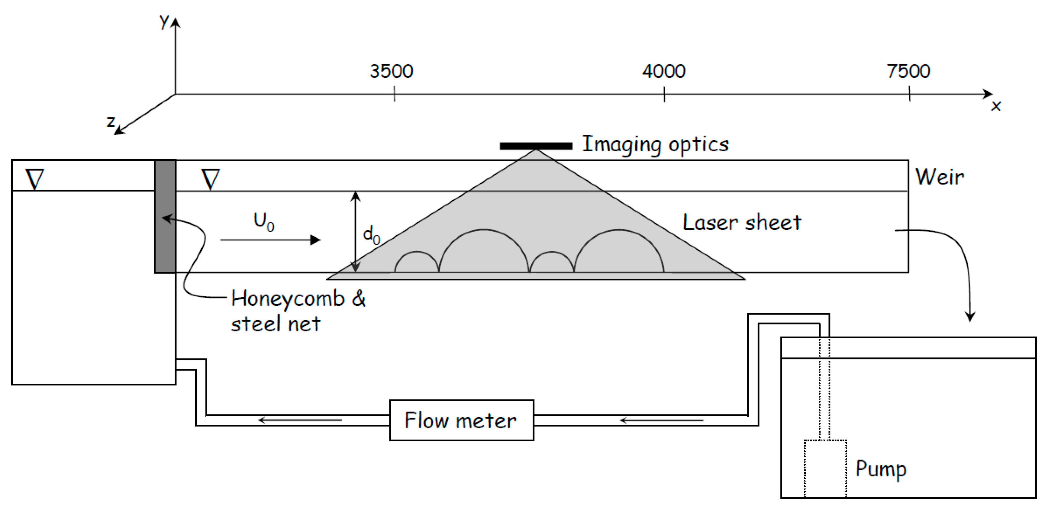
2.1. Water Flume

The experiments were conducted in a water flume with a smooth bottom and a length of 7.5 m and a cross-section of 0.295 m × 0.310 m. The steel base of the flume is flanked by two sets of glass planes. A honeycomb and a steel net were placed at the inlet of the water channel to obtain a uniform velocity distribution through the channel. The thickness of the honeycomb is 75 mm, and the diameter of the holes is 7.6 mm. The steel net used is made of a wire having a thickness of 0.8 mm forming 2.5 mm × 2.5 mm square holes. Water was pumped through the channel from a reservoir tank placed at the outlet that has a water storage capacity of 2 m³, and water is re-circulated back to the reservoir tank from the flume. A submersible pump controlled the flow rate, and the mean velocity in the channel was derived running PIV measurements on a channel without objects for several times as well as measured with a Corriolis flow meter. The temperature of the water was controlled to 20 °C using an automatic cooling arrangement. This is essential since variation in water temperature changes its viscosity and refractive index properties. Changes in water temperature may also lead to a displacement of the laser sheet and the plane of focus of the camera.

The water depth in the channel was maintained at 180 mm ± 1 mm for all measurement carried out. In order to minimize the reflections from the bottom of the water channel, a black-colored 2 mm thick Lexan plate with a width of 295 mm and length of 1500 mm was attached to the bottom. The edge of the plate was put at a distance of 3290 mm from the channel inlet, which is a distance judged sufficient to provide a steadily developed velocity profile in the area of interest. A schematic arrangement of the experimental set-up is presented in Figure 1.

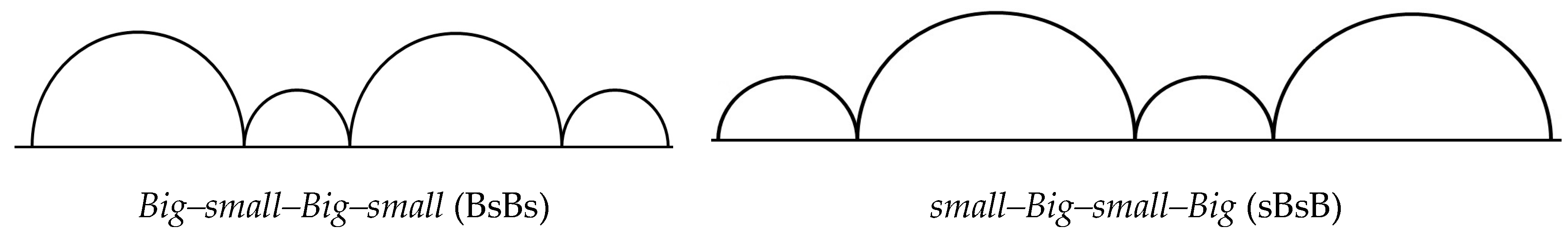
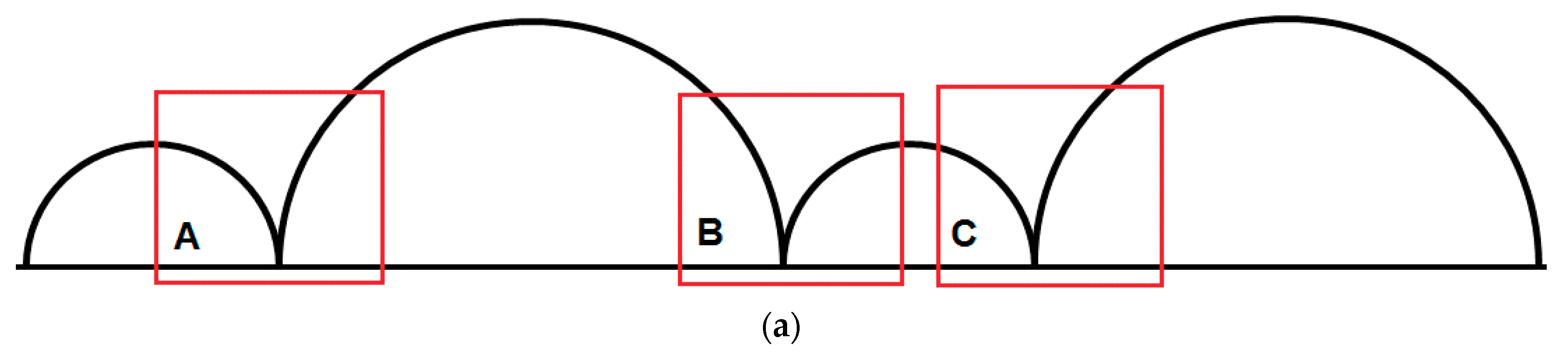
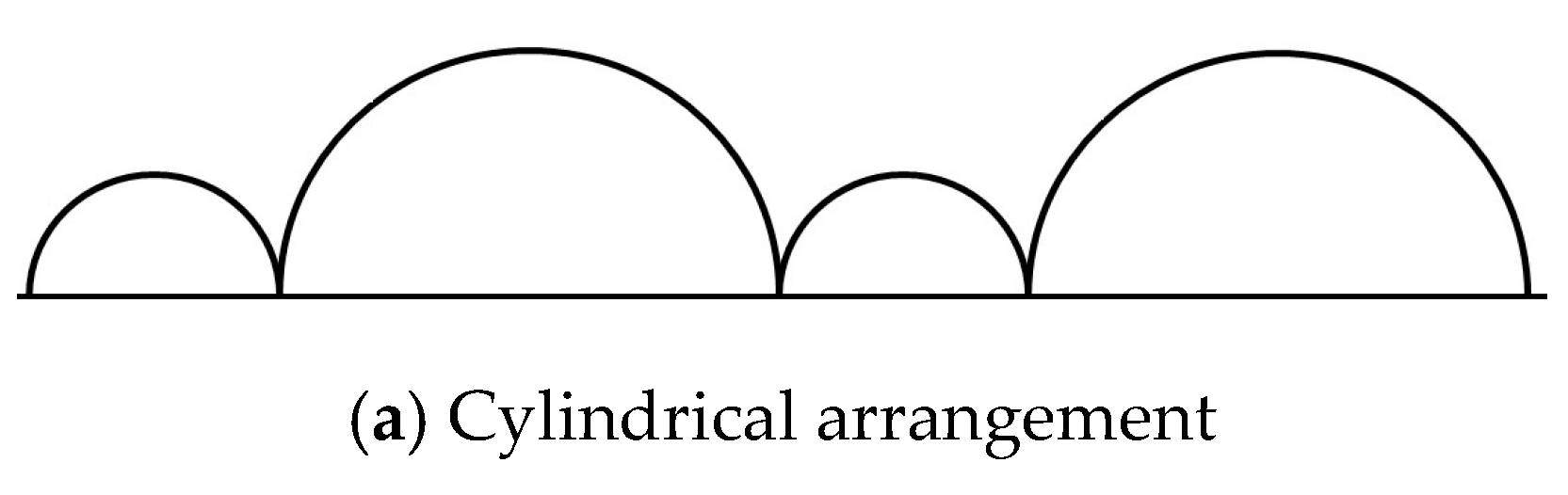
2.2. Arrangement of Half-Cylinders

To model embedded stones in a riverbed, half-cylinders were placed on the bottom of the water flume, as mentioned previously. The half-cylinders with a diameter of 100 mm and 200 mm were hollow polymethyl methacraylate(PMMA) with the same thickness, 3 mm and spanned the full width of the channel in order to reduce 3D effects. The shape of the half-cylinders was maintained by attaching a plate with the same length as the half-cylinder and a width corresponding to the inner diameter. Heavy weights were placed into the hollow regions formed by the half-cylinders in order to inhibit the arrangement from moving. To prevent water from seeping through the contact area between the bottom plate and the half-cylinders, silicon was used to seal the bottom edges of the half-cylinders. Furthermore, in order to avoid reflections from the half-cylinders, their surface was painted black. The half-cylinders were placed in two configurations according to big–small–big–small (BsBs) and small–big–small–big (sBsB), respectively; see Figure 2.

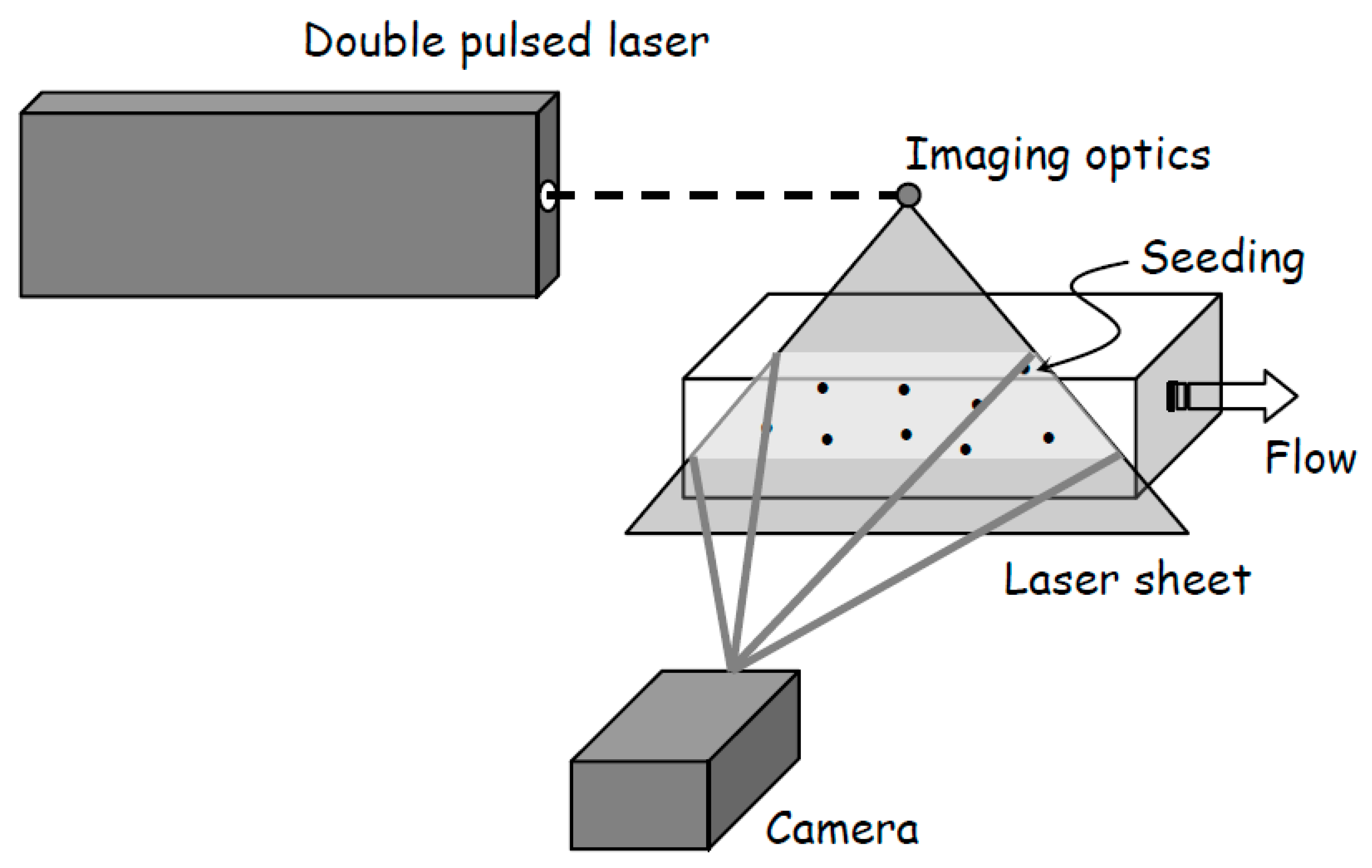
2.3. Experimental Technique (PIV)

PIV is a method to visualize and measure fluid flows in a two-dimensional plane [10,26,27,28]. A typical PIV setup consists of a light source which is usually a laser that illuminates the actual flow region of interest, forming a thin light sheet as shown in Figure 3. By seeding the fluid with small and neutral buoyant particles, the fluid motion can be measured as the particles pass the light sheet, being photographed by a high-speed camera. Each set of recordings consists of a number of double frame images that are divided into small regions called interrogation windows. Here, cross-correlation based on fast Fourier transform (FFT) is performed between the respective interrogation window in each frame resulting in a velocity vector field of the entire measured plane. Each vector represents the statistical mean velocity for the actual interrogation window [29] (Raffel et al., 2007). Generally, the tracer particles should not move more than a quarter of the interrogation window width in order to have an optimum correlation scheme [30] (Keane and Adrian, 1990).

The PIV system used in the present study is a commercially available system from Dantec Dynamics, consisting of a double-pulsed Nd:YAG L PIV laser from Litron having a maximum repetition rate of 100 Hz, and a FlowSense EO Camera with a spatial resolution of 1280 × 1024 pixels per frame. The laser is mounted on a maneuverable traverse, allowing the laser sheet and camera to shift position 600 mm in the x, y, and z-direction, respectively. However, the camera was manually rotated in both directions to obtain the PIV results in the normal direction to the curved surface, which was done using the trial and error method, enabling preview of DynamicStudio data acquisition software [31]. For the evaluation of τ, the field of view (FOV) was set to 16 × 16 mm², being the smallest possible FOV for the experimental setup where a Nikon micro NIKKOR 200 1:4D lens was used. In order to disclose flow features on a larger scale, an additional set of measurements were carried out with a FOV of 120 × 120 mm² now using a Nikon NIKKOR 24 1:2.8D lens. Since pulsed light was applied in all these PIV measurements, the shutter speed of the camera is irrelevant.

The seeding particles used in the present study are non-fluorescent hollow glass spheres from Dantec Dynamics A/S, having a diameter of 6 microns and a density allowing them to follow the motion of the flow [29] (Raffel et al., 2007).

A sample raw PIV image at point 5 of BsBs for U_∞ = 0.035 before the interrogation process (raw PIV image) is shown in Figure 4 along with its interrogation processed vector field where the field of view (FOV) was 16 × 16 mm².

2.4. Experimental Scenarios

The traverse used to maneuver the camera has a total working range of 0.6 m; considering this and the camera field of view, the full working range is ≈0.62 m. Hence, it is possible to do PIV measurements of the full geometry for both configurations.

Two free stream velocities were used for both arrangements, 0.035 m/s and 0.155 m/s; this corresponds to channel Reynolds numbers, Re, 3170 and 14,030, based on the hydraulic diameter of the channel, large cylinder Re 1950, 8650 based on the hydraulic radius of the large cylinder and channel Froude numbers, Fr, 0.026, 0.117, which mean that the flow for both cases is subcritical. The actual water level was kept constant at 0.18 m for all measurements avoiding disturbances, i.e., hydraulic jumps, on the free surface and also with respect to the volume of the tank. The laser sheet is applied from the top of the channel, and any disturbances on the free surface will have a negative effect on the quality of the laser sheet and, hence, the quality of the PIV measurements. This was minimized using a glass sheet over the free surface.

2.5. Error Analysis or Repeatability Test

Errors are mainly connected to the PIV measurements. Since PIV is a statistical method, the results are dependent on the sampling size and, generally, a large number of pictures generate results that are more accurate. For the present measurements, the sampling size was set to 1000 pictures, which is the maximum number for the PIV equipment used, and this sampling time was approximately 100 s. A repeatability test was conducted at four different times to find the differences in results at points where flow conforms with logarithmic velocity profiles. The largest difference (18%) was found close to the wall, and the error rapidly decreased when moving more than 1 mm away from the wall, and the smallest difference (0.9%) was found 5 mm away from the wall. The average difference between these repeated results was approximately 2%. The reason for the largest difference close to the wall may be traced to the uncertainty of the wall position and velocity fluctuations. Other errors, such as those generated by the measurements of flow rate and temperature and computations of averaged velocity, are assumed to be smaller. Further, the relatively low PIV Sampling rate (10 Hz) may introduce some errors, especially for the higher Re. These errors are still judged to be neglectable due to the long sampling time and since the dynamics of the flow is only studied for the lowest Re. It should also be noted that the velocity component in the z-direction is not measured. Neglecting this component, as done in this study, may, for instance, imply that the shear rate is underestimated. Additional errors also appear when the shear rate is derived, see Chapter 3.1.

3. Results and Discussion

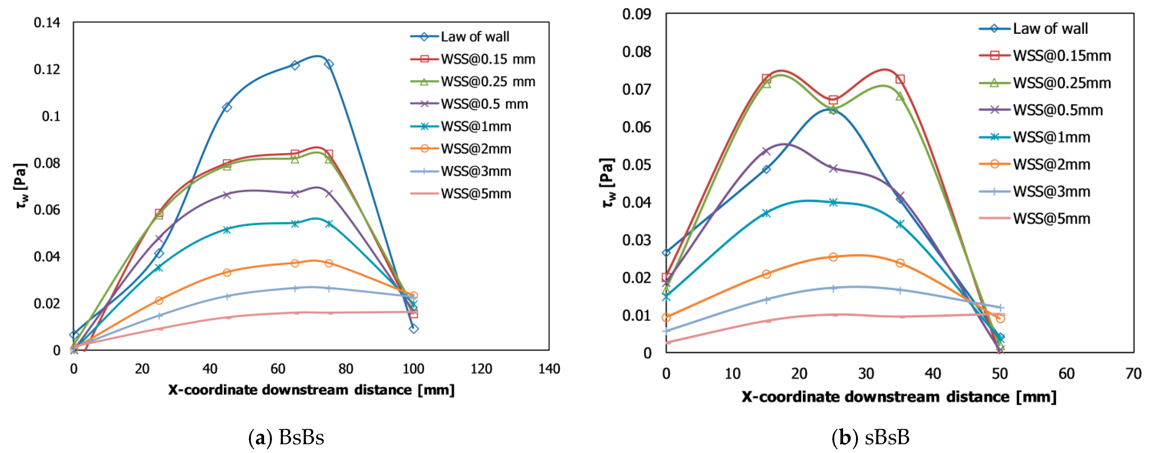
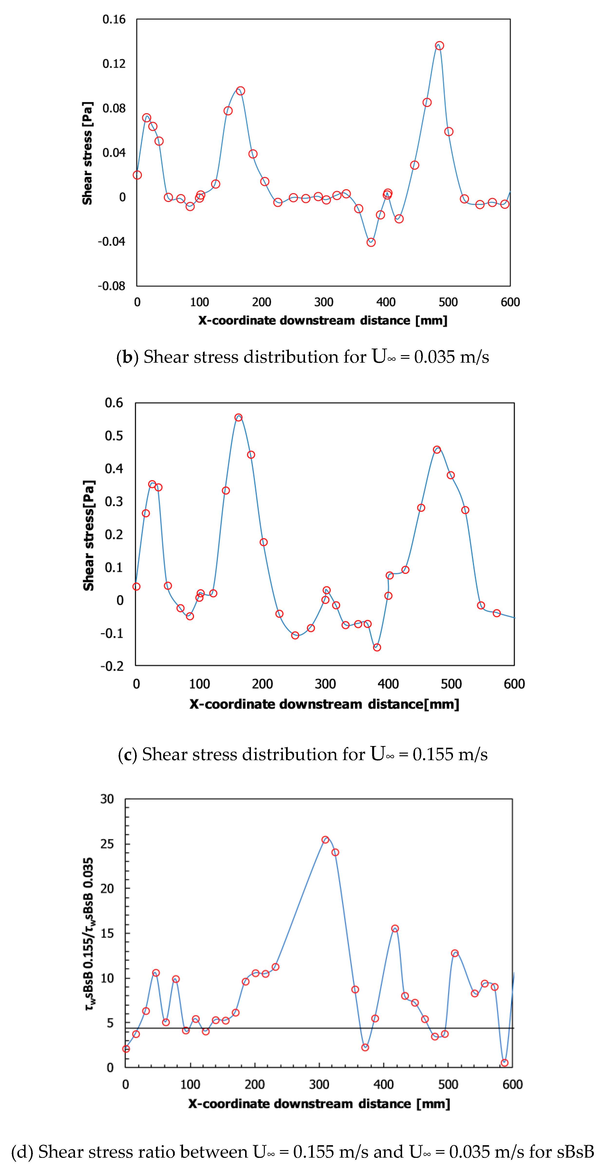
3.1. Shear Stress Analysis

The wall shear stress at the cylinder boundaries, τ_w, is defined as:

$${\tau }_{\mathrm{w}}=\mu {\frac{du}{dy}|}_{y=0}$$

(2)

where μ is the dynamic viscosity of the fluid and du/dy is the velocity gradient at the boundary.

Direct measurements of τ_w require accurate measurements of velocities inside the viscous sublayer, very close to the wall. This is not always possible, and one common technique is instead to determine the shear velocity u*, defined as ${\tau }_w=\rho u^{{*}^2}$, from the velocity profiles outside of the viscous sublayer [32,33,34,35]. For fully developed turbulent flows in pipes and channels, the dimensionless velocity profile can be described with the law of the wall, commonly expressed as:

$$u^{+}=y^{+}\hspace{1em}\mathrm{for} y^{+}<5$$

(3)

$$u^{+}=\frac{1}{\kappa }\ln \left(\frac{y}{y_0}\right)\hspace{1em}\mathrm{for} y^{+}>30$$

(4)

where $u^{+}=u/u^{*}$, y⁺ is the dimensionless distance from the wall defined as $y^{+}=y{u}^{*}/\nu$, κ is von Karman’s constant which is 0.41, and y₀ is the roughness height [36,37], which is set to 0.05 mm [33], which corresponds to the roughness height of plastic material. By assuming that the boundary layer on the first half of the most upstream cylinder has a similar velocity distribution, it is possible to calculate the friction velocity from the measured mean velocity in the logarithmic layer and the logarithms of y and solve for u* [38]. By using this procedure, τ_w on the surfaces of the first half of the first cylinder for both cylindrical arrangements and U_∞ = 0.035 m/s is plotted, see Figure 5 and the curve denoted Law of Wall. KX Whipple [39,40] described the regression process for this method to derive wall shear stress in detail. Since the flow can only be treated as fully developed in the beginning of the arrangements, the wall shear stress from the regression method was only calculated at five (sBsB) and six points (BsBs) on the first half of the first cylinder. The wall shear stress was also derived directly from the velocity gradient at 0.15, 0.25, 0.5, 1, 2, 3, and 5 mm distance from the wall at the same points, assuming a linear relationship according to Equation (2), see Figure 5. The differences in computed wall shear stress at 0.15 mm and 0.25 mm are small, only about 2.1% in average, and hence, the velocity profiles are close to linear up to 0.25 mm, see Figure 6, which shows the velocity profile just before the midpoint of the first big cylinder for the BsBs case with U_∞ = 0.035 m/s. At larger distances, the computed τ_w becomes smaller, since the distance from the wall is in the logarithmic layer and the assumption of a linear profile fails. Therefore, τ_w was derived based on the velocity at a distance of 0.25 mm from the wall assuming a linear velocity profile up to this point. A comparison between this approach and the theoretical curve for a fully developed logarithmic velocity profile shows that the latter frequently used approach (i.e., [30,31,32]) gives a fair approximation, but as shown in Figure 5, there are some differences due to the complex geometry resulting in a non-developed flow. Hence, if possible, the shear stress should be derived from measurements of velocity very close to the bottom assuming a linear relationship up to the point of measurement. In addition, Figure 6 shows the velocity profile close to the wall at point 3 (3rd point in the Figure 5a from 0 x-coordinate downstream distance) for the case of BsBs for U_∞ = 0.035 m/s in scaled units, and it can be seen that the same regions that are typical for a “law of the wall” boundary layer can be identified at this point.

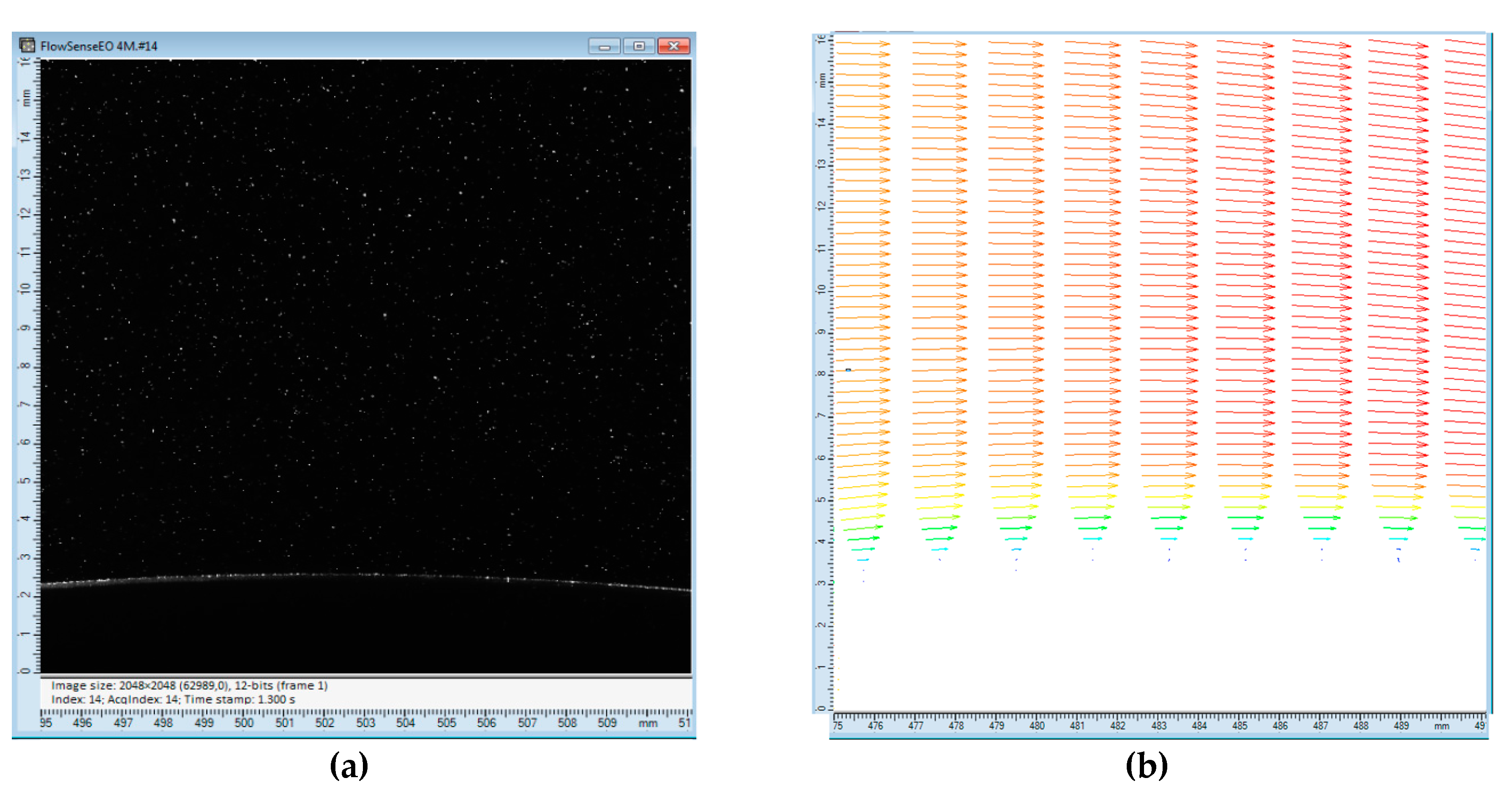
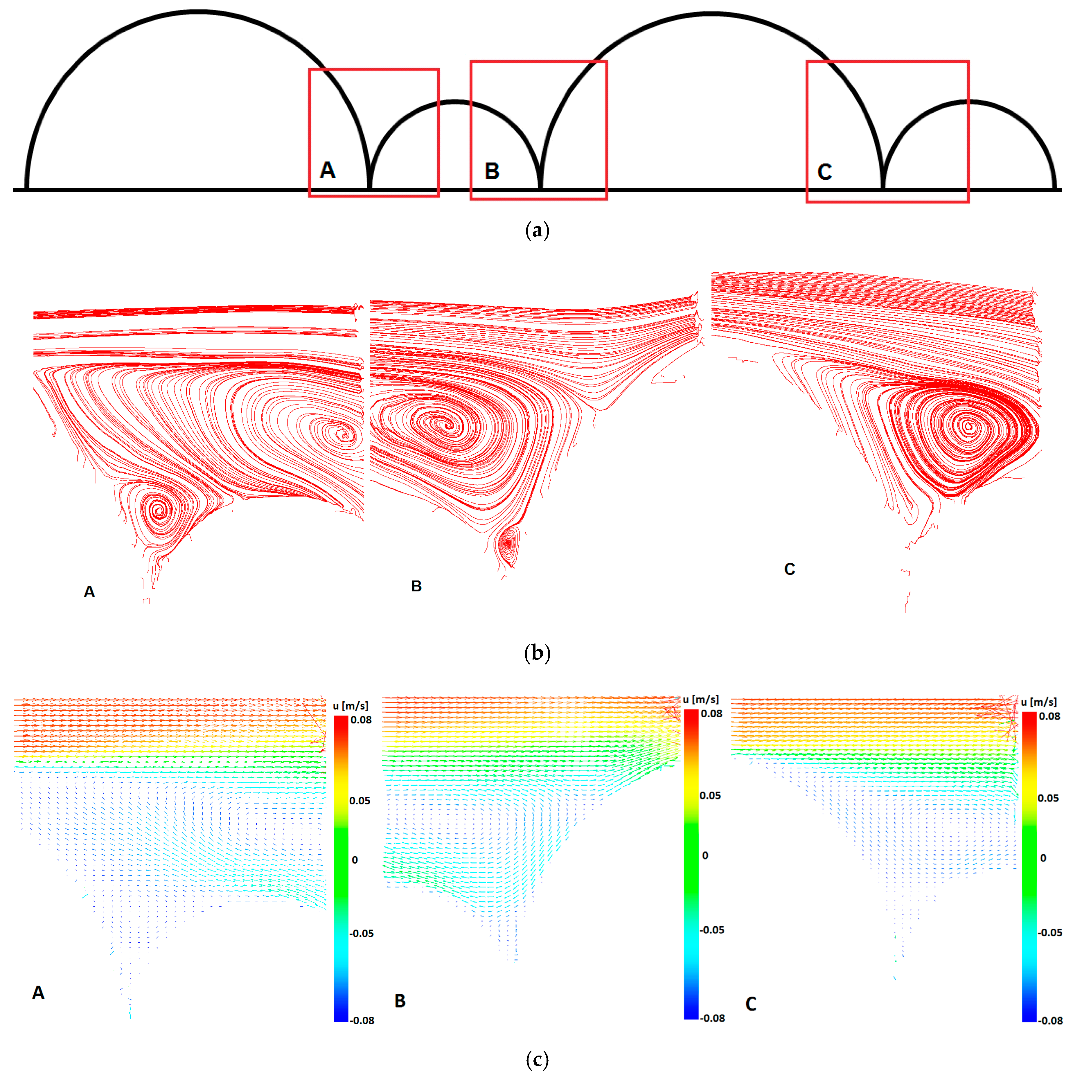
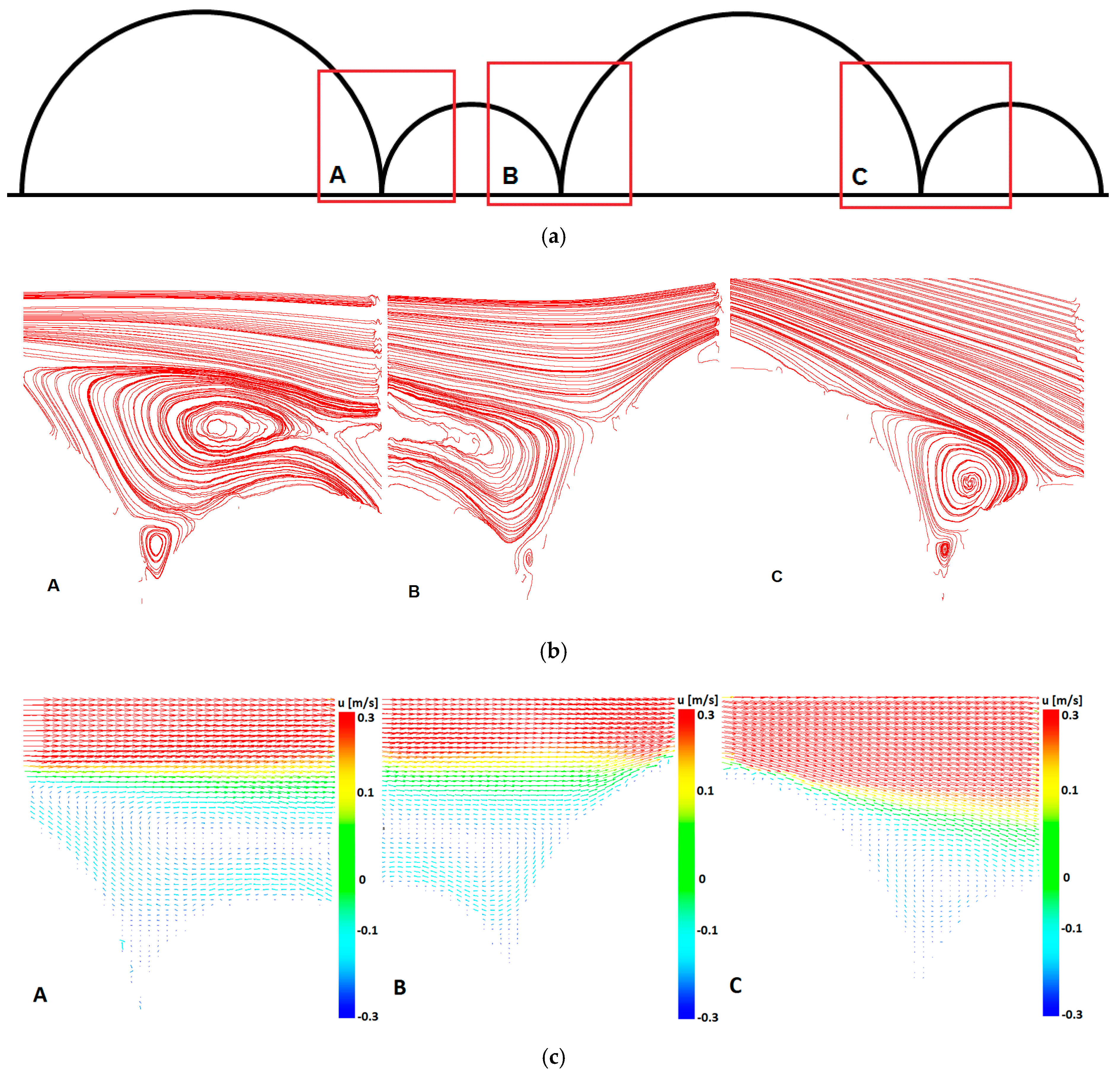
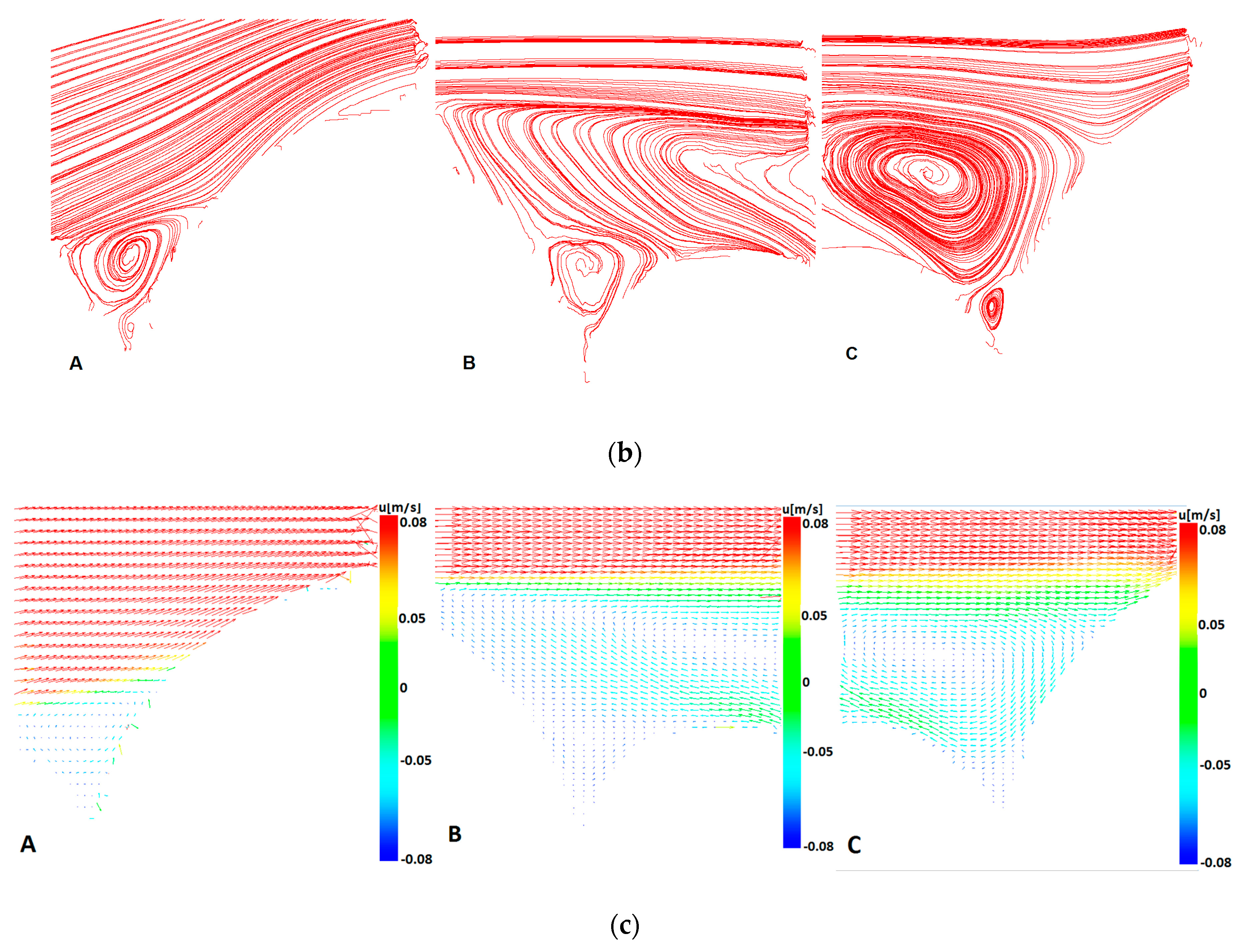
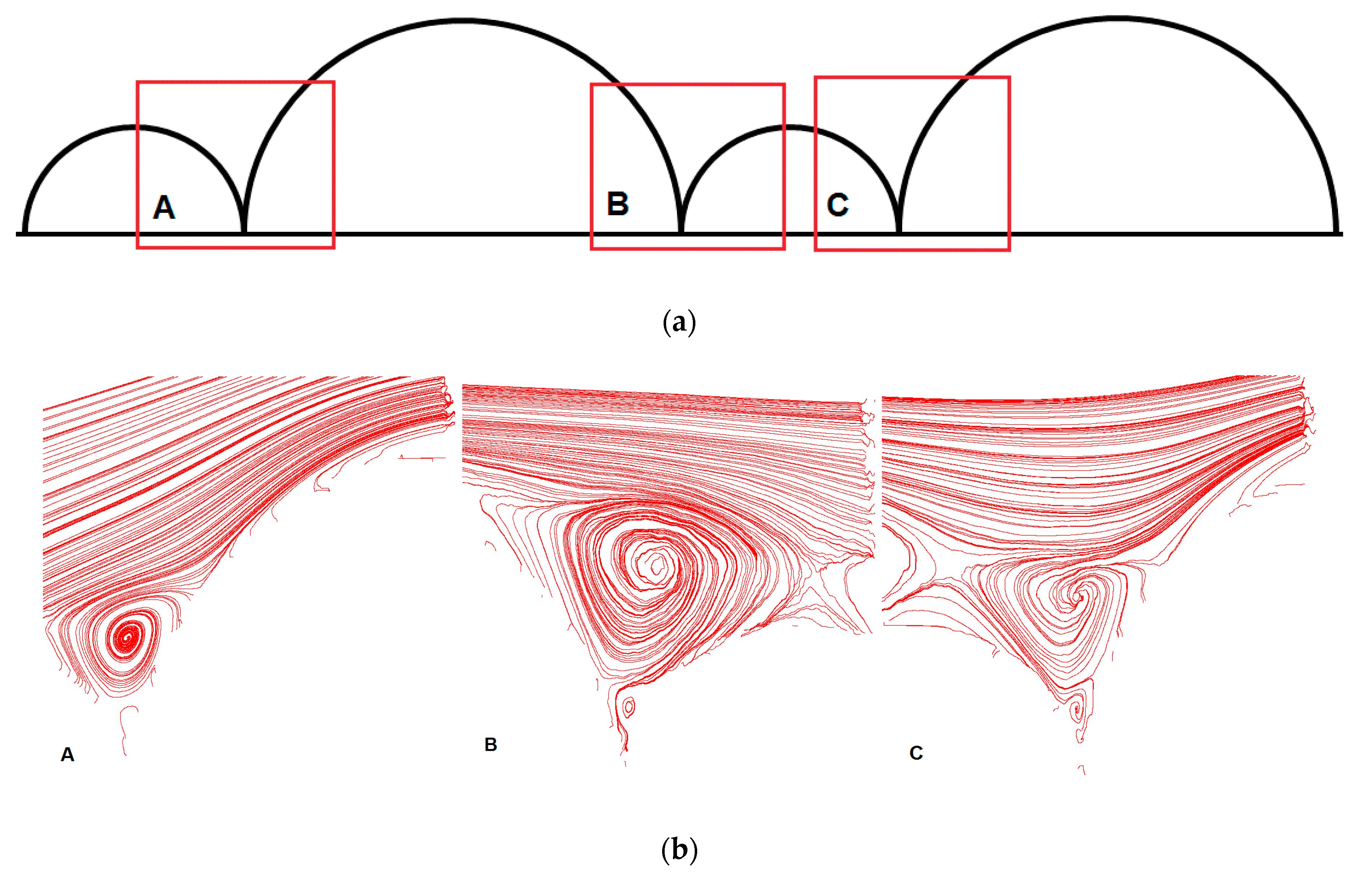
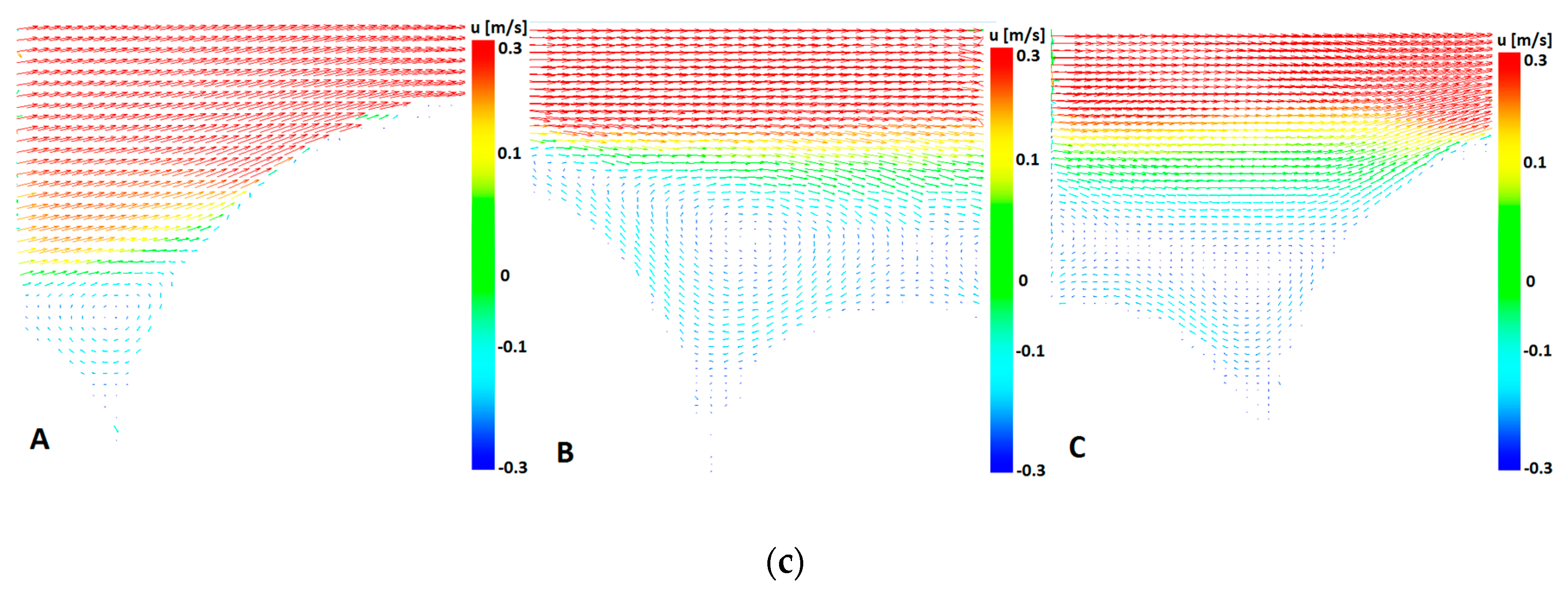
3.2. Time-Averaged Streamlines and Vector Fields

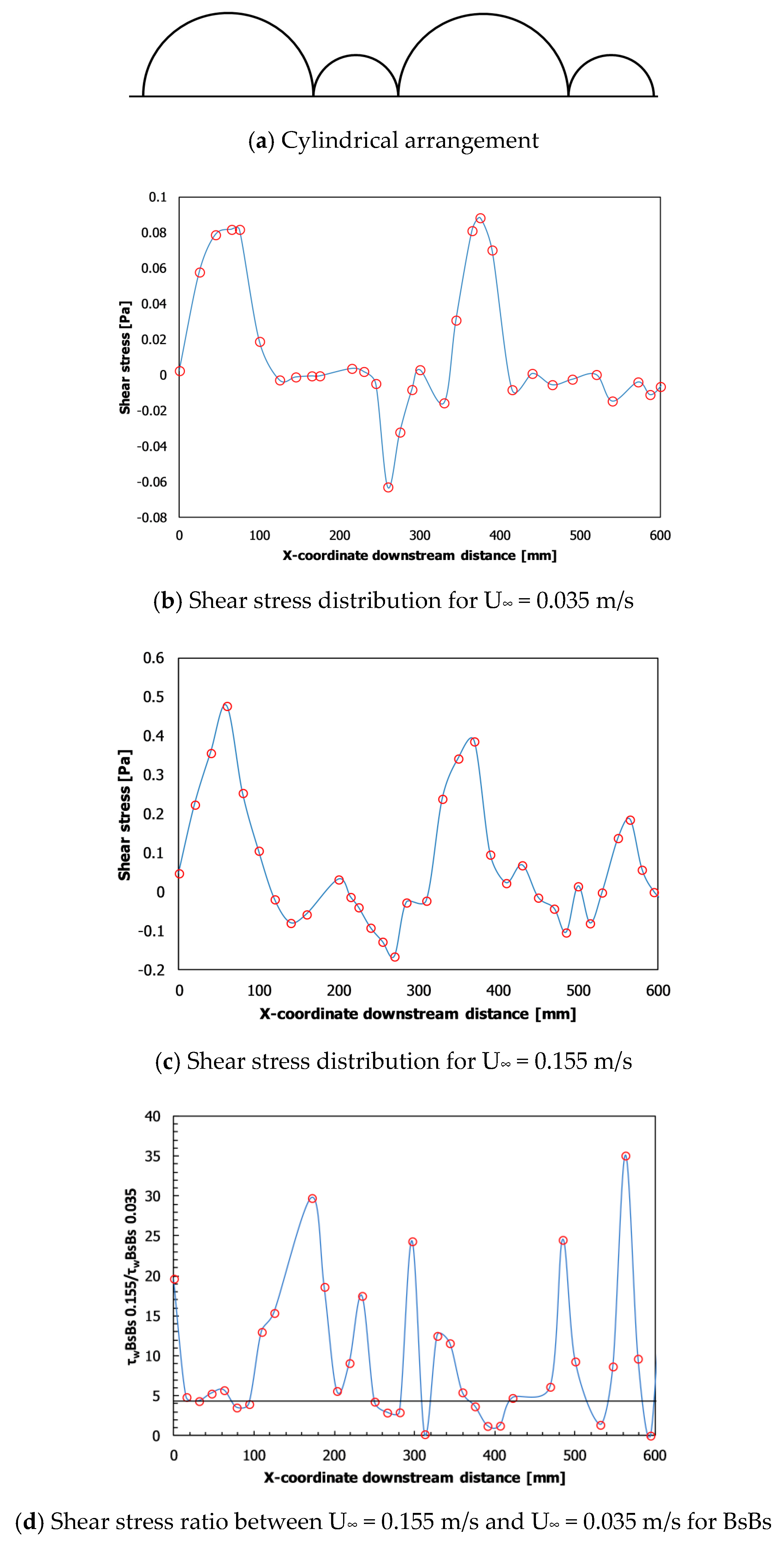
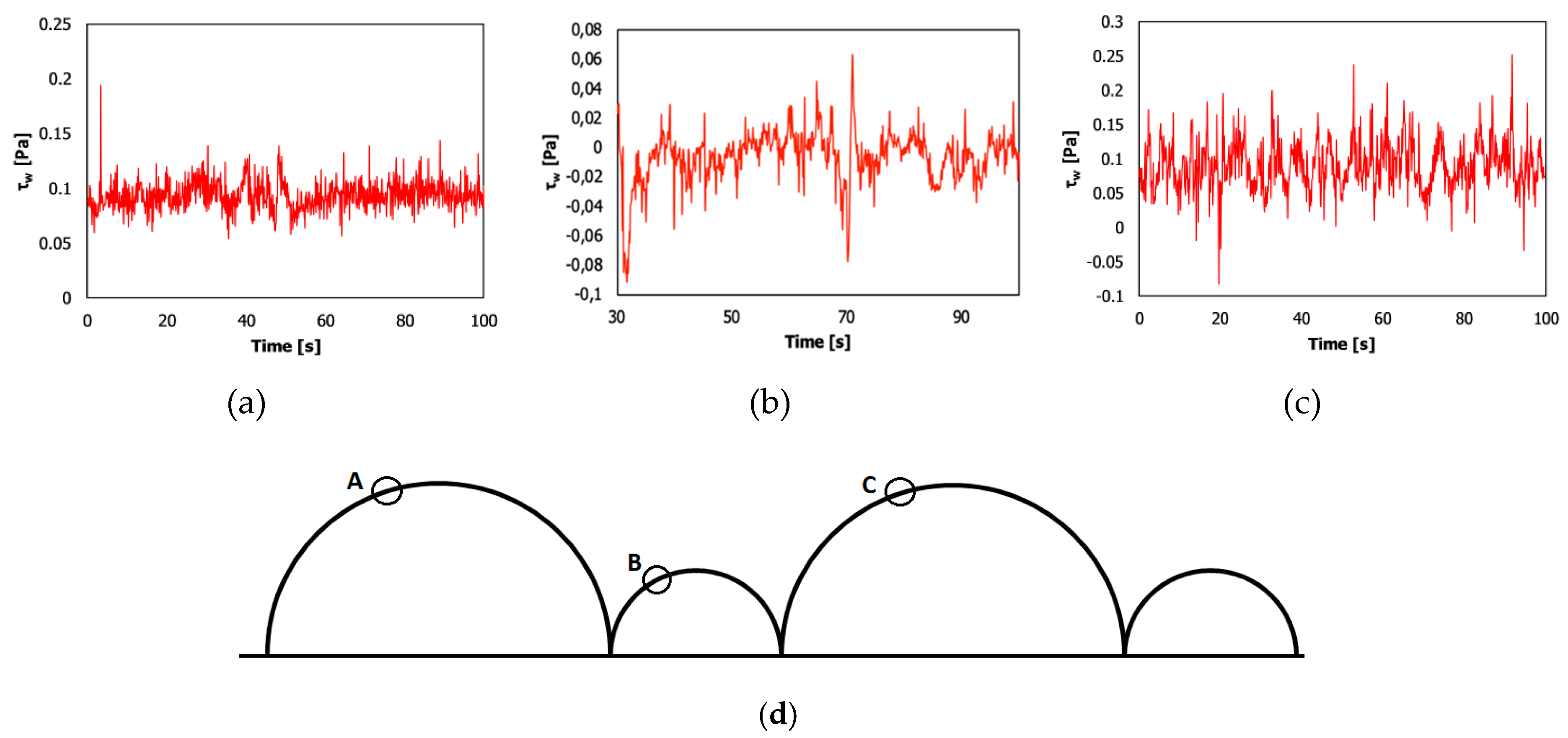
Before presenting the results of the shear stress at the wall, time-averaged velocity fields at certain areas will be presented. Figure 7, Figure 8, Figure 9 and Figure 10 show the streamlines and vector fields for both the BsBs and sBsB cases at different locations along the half-cylinder configuration for the two different mean free stream velocities: U_∞ = 0.035 m/s and U_∞ = 0.155 m/s for each case. Main flow direction is from left to right, and notice that Figure 7a, Figure 8a, Figure 9a, and Figure 10a show the area where streamlines and vector fields were captured with PIV.

A main characteristic for all cases is a high-speed flow field on the top of the cylinders. This is shown by the streamlines as well as the red arrows in the velocity field. For the higher Re, this flow moves a little bit deeper into the spaces between the cylinders. Another main feature is the recirculation zones, vortices, formed between the cylinders. For both cases, these zones change in shape as Re increases. It can also be noted that the velocity of these circulations is relatively low.

3.3. Shear Stress

The distributions of τ_w over the semi-circular cylinders are shown in Figure 11 and Figure 12, where Figure 11a and Figure 12a show how the cylinders are arranged and Figure 11b,c and Figure 12b,c show τ_w as a function of position for the two free stream velocities, respectively.

It is seen from Figure 11b that, for the BsBs case, τ_w gradually increases as the flow is directed upwards at the first cylinder until its mid-point where τ_w is at its maximum. The rapid decrease that follows indicates that the flow detaches from the cylinder, forming a rather large area with a low τ_w being in agreement with Figure 7. The negative extreme value in Figure 11b that follows is a result of the recirculation zone shown in Figure 7. The second positive extreme value is due to the fact that the high-speed flow field attaches to the larger cylinder. This field detaches again and does not reach down to the smaller cylinder that follows and, since the recirculation that forms in the beginning of the last cylinder is not strong, τ_w becomes small. For the higher Re, τ_w increases considerably, see Figure 11c. Otherwise, τ_w behaves in a similar manner except on the final cylinder where there is an additional extreme value probably caused by the high-speed flow field approaching this cylinder, see Figure 8.

For the sBsB cases, τ_w behaves in a similar way. To exemplify, for both arrangements, the maximum of τ_w is at the second big cylinder for the low Re, while it is at the first big cylinder for the high Re, see Figure 11 and Figure 12. This may be an inertia effect, meaning that the flow is to a larger extent deflected away from the arrangement at the higher Re.

In order to quantify the effect of increasing the free stream velocity from U_∞ = 0.035 m/s to U_∞ = 0.155 m/s, the absolute value of ratios when dividing τ_w for the lager velocity with that of the lower is shown in Figure 11d and Figure 12d. The ratio in U_∞ = 4.4 is plotted in the figures for comparison. It is seen that these ratios of τ_w are close to 4.4 until half of the first big cylinder for the BsBs case, Figure 11d. Then it increases in value in the first recirculation zone where the flow speed is low, and it continues to vary in the recirculation zone. The ratios of τ_w become close to 4.4 again around the midpoint of the second large cylinder as the flow starts being regular there, but the τ_w ratio fluctuates again in the next recirculation zone. The largest τ_w ratio is found where flows are low or reverse. The τ_w ratio for sBsB, as shown in Figure 12d, behaves in a similar manner, and it can be concluded that the τ_w ratio between the different flow rates is directly dependent on the free stream velocity ratio when the flow is not detached from the cylinders. However, in the recirculation zones, the τ_w ratio can be influenced to a larger extent. This is nearly always due to the fact that both τ_w are small. There is also a small error introduced in the evaluation. Measuring exactly at few points for two flow cases was very difficult to maintain; there could therefore be small changes in the position of the measuring points contributing to the extreme τ_w ratio in a few points.

Until now, focus has been on mean values of τ_w. Due to phenomena like turbulence and shedding, τ_w will be time-dependent, see Figure 13, being time-resolved τ_w for three points. As seen, the time-dependent appearance of τ_w is different for the three points. Most characteristic are the peaks for point B located in the recirculation zone. Comparing these peaks to those obtained for points A and C reveals that the peaks for point B are based on single values, while those obtained for points A and C are built from several points.

From

Table 1. Extreme values of τ_w and SD at points over BsBs for 0.035 m/s flow case.

Points over BsBs	A	B	C
τwmean (Pa)	0.094	−0.0046	0.090
τwmax (Pa)	0.19	0.062	0.25
τwmax/τwmean	2.1	−13	2.8
τwmin (Pa)	0.055	−0.092	−0.0826
τwmin/τwmean	0.58	20	−0.91
SDτw	0.013	0.017	0.037
SDτw/τwmean	0.14	−3.6	0.41

, it is seen that ratios between τ_wmax and τ_wmean and τ_wmin and τ_wmean are significantly higher for point B compared to other points A and C. This is because this is the recirculation area where flow speed is mostly low, but sudden large fluctuation leads to τ_w becoming high. Thus, even if flow rate is constant, there can be sudden changes in τ_w in the low velocity areas. This is obviously important for the benthic fauna. The standard deviation (SD) of τ_w at point A is significantly low compared to the other two points, and the ratio between SDτ_w and τ_wmean is also smaller than that of the other two points B and C if the values are absolute. As a low standard deviation means that most measured values are very close to the mean, while high standard deviation means that measured values are spread out from mean [41], measured values at point A are very close to mean but measure values at further downward points increase gradually as the flow field is complex where recirculation occurs.

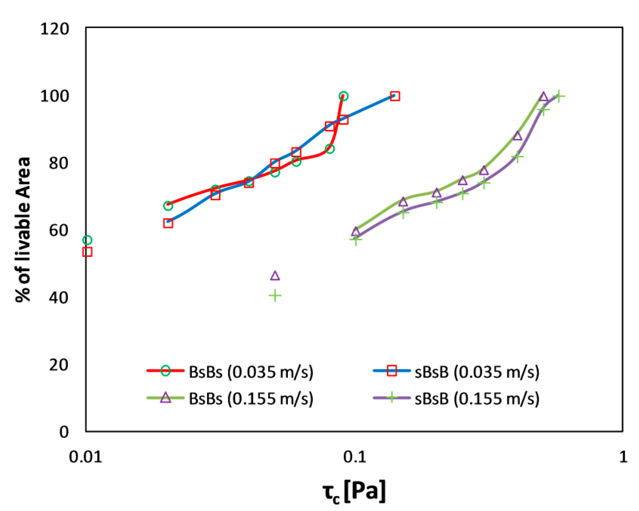
3.4. Critical Shear Stress

Livable areas of species are here defined as the areas in the bottom of the river where a certain species is able to maintain their position in the riverbed at a specific flow rate. By assuming that the wall shear stress is the restricting parameter, the livable area for a species can be calculated as the area where the absolute value of τ_w is below the species critical value τ_c. The ratio of livable area in this experimental set-up for different values of τ_c (which could be related to different species) is plotted in Figure 14 for the two mean free stream velocities. Absolute values of τ_w are used, since the resistance of the species to τ_w is independent on direction. The trend is the same for all experimental scenarios where the percentage of the bottom surface being livable increases fastest with τ_c in the beginning for both mean free stream velocities. An interesting observation is that the influence of arrangement of the half-cylinders (BsBs or sBsB) is small, with a slight trend that the BsBs arrangement creates a larger percentage livable area. It is also obvious that the % livable area is dependent on the free stream velocity. To exemplify, for species with τ_c = 0.1 Pa, the percentage livable area for the BsBs arrangement is 100% and about 60% for U_∞ = 0.035 m/s and U_∞ = 0.155 m/s, respectively.

4. Conclusions

In this paper, the flow around half-cylinders at the bottom of an open channel was measured using particle image velocimetry (PIV). The main objective was in addition to the main flow characteristics near the bottom, to investigate the distribution of shear stress along the bottom objects. The key question addressed was how shear stress changes in the livable area on the half-cylinder configuration. It was shown that the flow pattern is dominated by vortical structures between the half-cylinders and on the leading and trailing sides of the cylinder sets. It was shown that the regression method that calculates wall shear stress from the measured velocities in the logarithmic boundary layer predicts the correct order of magnitude but differs for measurement points along the first cylinder in the investigated simplified stone configuration. This indicates that direct measurements of near wall velocity gradients are necessary to accurately calculate the wall shear stress for more complex geometries. Considering a critical shear stress, it is shown that the trend is close to identical for all experimental scenarios with a percentage of the bottom surface being livable where critical shear stress varies significantly for different mean free stream velocities. The changes in wall shear stress as a function of arrangement, free stream velocity, and time implies habitat heterogeneity, allowing benthic invertebrates with different shear stress tolerance to exist when the bottom consists of differently sized stones [5], which can be an addition to available research work. The variation in time also enables adequate nutrition and oxygen [4].

Future work may consider additional measurements possible with stereoscopic [42] or tomographic PIV [43] in lab to capture 3D effects when, for instance, introducing artificial structures [9] (Jeffries and Mills, 1990) and measurement in field.

References

1. Hynes, H.B.N. The Ecology of Running Waters; Liverpool University Press: Liverpool, UK, 1970; Volume 555. [Google Scholar]
2. Poff, N.L.; Zimmerman, J.K. Ecological responses to altered flow regimes: A literature review to inform the science and management of environmental flows. Freshw. Biol. 2010, 55, 194–205. [Google Scholar] [CrossRef]
3. Alfredsen, K. An Assessment of Ice Effects on Indices for Hydrological Alteration in Flow Regimes. Water 2017, 9, 914. [Google Scholar] [CrossRef]
4. Mérigoux, S.; Dolédec, S. Hydraulic requirements of stream communities: A case study on invertebrates. Freshw. Biol. 2004, 49, 600–613. [Google Scholar] [CrossRef]
5. Allan, J.D.; Castillo, M.M. Stream Ecology: Structure and Function of Running Waters; Springer Science & Business Media: Heidelberg, Germany, 2007. [Google Scholar]
6. Doledec, S.; Lamouroux, N.; Fuchs, U.; Merigoux, S. Modelling the hydraulic preferences of benthic macroinvertebrates in small European streams. Freshw. Biol. 2007, 52, 145–164. [Google Scholar] [CrossRef]
7. Asad, B.; Sayeed, S.M.; Lundström, S.; Andersson, A.; Hellström, G. A Review of Particle Image Velocimetry for Fish Migration. World J. Mech. 2016, 6, 131–149. [Google Scholar] [CrossRef]
8. Bockelmann-Evans, B.N.; Davies, R.; Falconer, R.A. Measuring bed shear stress along vegetated river beds using FST-hemispheres. J. Environ. Manag. 2008, 88, 627–637. [Google Scholar] [CrossRef]
9. Jeffries, M.; Mills, D.M. Freshwater Ecology Principles and Applications; Belhaven Press: London, UK, 1990. [Google Scholar]
10. Green, T. Particle Image Velocimetry in Practice. Ph.D. Thesis, Luleå University of Technology, Luleå, Sweden, September 2009. [Google Scholar]
11. Green, T.M.; Lindmark, E.M.; Lundström, T.S.; Gustavsson, L.H. Flow characterization of an attraction channel as entrance to fishways. River Res. Appl. 2011, 27, 1290–1297. [Google Scholar] [CrossRef]
12. Sayeed-Bin-Asad, S.; Lundström, T.; Andersson, A. Experimental study of the flow past submerged half-cylinders. AIP Conf. Proc. 2017. [Google Scholar] [CrossRef]
13. Wassvik, E. Model test of an efficient fish lock as an entrance to fish ladders at hydropower plants. Master’s Thesis, Luleå University of Technology, Luleå, Sweden, May 2004. [Google Scholar]
14. Tritico, H.; Cotel, A.; Clarke, J. Development, testing and demonstration of a portable submersible miniature particle imaging velocimetry device. Meas. Sci. Tech. 2007, 18, 2555. [Google Scholar] [CrossRef]
15. Bouckaert, F.W. Microflow regimes and the distribution of macroinvertebrates around stream boulders. Freshw. Biol. 1998, 40, 77–86. [Google Scholar] [CrossRef]
16. Lohrmann, A.; Cabrera, R.; Kraus, N.C. Acoustic-Doppler velocimeter (ADV) for laboratory use. In Fundamentals and Advancements in Hydraulic Measurements and Experimentation; ASCE: Buffalo, NY, USA, 1994. [Google Scholar]
17. Gibbins, C.; Vericat, D.; Batalla, R.J. When is Stream Invertebrate Drift Catastrophic? The Role of Hydraulics and Sediment Transport in Initiating Drift during Flood Events. Freshw. Biol. 2007, 52, 2369–2384. [Google Scholar] [CrossRef]
18. Gibbins, C.; Batalla, R.J.; Vericat, D. Invertebrate drift and benthic exhaustion during disturbance: Response of mayflies (Ephemeroptera) to increasing shear stress and river-bed instability. River Res. Appl. 2010, 26, 499–511. [Google Scholar] [CrossRef]
19. Driest, E.V. On turbulent flow near a wall. J. Aeronaut. Sci. 1956, 23, 1007–1011. [Google Scholar] [CrossRef]
20. Pope, S.B. Turbulent flows. Meas. Sci. Tech. 2001, 12. [Google Scholar] [CrossRef]
21. Sundstrom, L.J.; Cervantes, M.J. Characteristics of the wall shear stress in pulsating wall-bounded turbulent flows. Exp. Therm. Fluid Sci. 2018, 96, 257–265. [Google Scholar] [CrossRef]
22. He, S.; Ariyaratne, C.; Vardy, A. Wall shear stress in accelerating turbulent pipe flow. J Fluid Mech. 2011, 685, 440–460. [Google Scholar] [CrossRef]
23. Sundström, J. Studies of Transient and Pulsating flows with application to Hydropower. Ph.D. Thesis, Luleå University of Technology, Luleå, Sweden, April 2018. [Google Scholar]
24. Song, S.; DeGraaff, D.B.; Eaton, J.K. Experimental study of a separating, reattaching, and redeveloping flow over a smoothly contoured ramp. Int. J. Heat Fluid Flow 2000, 21, 512–519. [Google Scholar] [CrossRef]
25. Sundstrom, L.J.; Mulu, B.G.; Cervantes, M.J. Wall friction and velocity measurements in a double-frequency pulsating turbulent flow. J. Fluid Mech. 2016, 788, 521–548. [Google Scholar] [CrossRef]
26. Khayamyan, S.; Lundström, T.S.; Hellström, J.G.I.; Gren, P.; Lycksam, H. Measurements of transitional and turbulent flow in a randomly packed bed of spheres with particle image velocimetry. Transp. Porous Media 2017, 116, 413–431. [Google Scholar]
27. Saber, A.; Lundström, S.; Hellström, G. Influence of Inertial Particles on Turbulence Characteristics in Outer and Near Wall Flow as Revealed with High Resolution Particle Image Velocimetry. J. Fluids Eng. 2016, 138, 091303. [Google Scholar] [CrossRef]
28. Larsson, I.S.; Johansson, S.P.; Lundström, T.S.; Marjavaara, B.D. PIV/PLIF experiments of jet mixing in a model of a rotary kiln. Exp. Fluids 2015, 56, 111. [Google Scholar] [CrossRef]
29. Raffel, M.; Willert, C.E.; Kompenhans, J. Particle Image Velocimetry: A Practical Guide; Springer: Berlin, Germany, 2013. [Google Scholar]
30. Keane, R.D.; Adrian, R.J. Optimization of particle image velocimeters. I. Double pulsed systems. Meas. Sci. Tech. 1990, 1, 1202. [Google Scholar]
31. Asad, B.; Sayeed, S. Laser Based Flow Measurements to Evaluate Hydraulic Conditions for Migrating Fish and Benthic Fauna. Ph.D. Thesis, Luleå University of Technology, Luleå, Sweden, April 2019. [Google Scholar]
32. Wilcock, P.R. Estimating local bed shear stress from velocity observations. Water Resour. Res. 1996, 32, 3361–3366. [Google Scholar] [CrossRef]
33. Smart, G.M. Turbulent velocity profiles and boundary shear in gravel bed rivers. J. Hydraul. Eng. 1999, 125, 106–116. [Google Scholar] [CrossRef]
34. Bagherimiyab, F.; Lemmin, U. Shear velocity estimates in rough-bed open-channel flow. Earth Surf. Process. Landf. 2013, 38, 1714–1724. [Google Scholar] [CrossRef]
35. Hoover, T.M.; Ackerman, J.D. Near-bed hydrodynamic measurements above boulders in shallow torrential streams: Implications for stream biota. J. Environ. Eng. Sci. 2004, 3, 365–378. [Google Scholar] [CrossRef]
36. Nakae, H.; Inui, R.; Hirata, Y.; Saito, H. Effects of surface roughness on wettability. Acta Mater. 1998, 46, 2313–2318. [Google Scholar] [CrossRef]
37. Gadelmawla, E.; Koura, M.M.; Maksoud, T.M.A.; Elewa, I.M.; Soliman, H.H. Roughness parameters. J. Mater. Process. Tech. 2002, 123, 133–145. [Google Scholar] [CrossRef]
38. Bergeron, N.E.; Abrahams, A.D. Estimating shear velocity and roughness length from velocity profiles. Water Resour. Res. 1992, 28, 2155–2158. [Google Scholar] [CrossRef]
39. Whipple, K.X. Bedrock rivers and the geomorphology of active orogens. Annu. Rev. Earth Planet. Sci. 2004, 32, 151–185. [Google Scholar] [CrossRef]
40. Brocklehurst, S.H.; Whipple, K.X. Assessing the relative efficiency of fluvial and glacial erosion through simulation of fluvial landscapes. Geomorphology 2006, 75, 283–299. [Google Scholar] [CrossRef]
41. Altman, D.G.; Bland, J.M. Standard deviations and standard errors. BMJ 2005, 331, 903. [Google Scholar] [CrossRef]
42. Khayamyan, S.; Lundström, T.S.; Gren, P.; Lycksam, H.; Hellström, J.G.I. Transitional and turbulent flow in a bed of spheres as measured with stereoscopic particle image velocimetry. Transp. Porous Media 2017, 117, 45–67. [Google Scholar]
43. Larsson, I.S.; Lundström, T.S.; Lycksam, H. Tomographic PIV of flow through ordered thin porous media. Exp. Fluids 2018, 59, 96. [Google Scholar] [CrossRef]
Figure 1. Schematic arrangement of the experimental set-up.
Water 11 00650 g001
Figure 2. Half-cylinder arrangements.
Water 11 00650 g002
Figure 3. PIV measurement setup consisting of a double-pulsed laser, imaging optics forming the laser sheet, and camera for recording.
Water 11 00650 g003
Figure 4. Particle image velocimetry (PIV) image at point 5 of BsBs for U = 0.035: (a) Raw PIV image, (b) processed vector field.
Water 11 00650 g004
Figure 5. Shear stress distribution over the first half of upstream cylinder.
Water 11 00650 g005
Figure 6. Boundary layer velocity profile at point 3 of the first big cylinder for BsBs and U = 0.035 m/s.
Water 11 00650 g006
Figure 7. Streamline and vector fields for BsBs and U = 0.035 m/s: (a) Area of interest (b) streamlines (c) vector fields.
Water 11 00650 g007
Figure 8. Streamline and vector fields for BsBs and U = 0.155 m/s: (a) Area of interest (b) streamlines (c) vector fields.
Water 11 00650 g008
Figure 9. Streamline and vector fields for sBsB and U = 0.035 m/s: (a) Area of interest (b) streamlines (c) vector fields.
Water 11 00650 g009aWater 11 00650 g009b
Figure 10. Streamline and vector fields for sBsB and U = 0.155 m/s: (a) Area of interest (b) streamlines (c) vector fields.
Water 11 00650 g010aWater 11 00650 g010b
Figure 11. Shear stress distribution for BsBs.
Water 11 00650 g011
Figure 12. Shear stress distribution for sBsB.
Water 11 00650 g012aWater 11 00650 g012b
Figure 13. Fluctuation of shear stress for BsBs with U = 0.035 m/s: (a) τw at A; (b) τw at B; (c) τw at C; (d) measured points.
Water 11 00650 g013
Figure 14. Percentage of the total bottom objects having a shear stress value (τ) lower than a critical value (τc) [being livable (τ < τc)] as a function of the flow velocity and cylinder arrangement. N.B: X-axis is in logarithmic scale.
Water 11 00650 g014