Assessing the Impact of Reservoir Parameters on Runoff in the Yalong River Basin using the SWAT Model

Abstract

The construction and operation of cascade reservoirs has changed the natural hydrological cycle in the Yalong River Basin, and reduced the accuracy of hydrological forecasting. The impact of cascade reservoir operation on the runoff of the Yalong River Basin is assessed, providing a theoretical reference for the construction and joint operation of reservoirs. In this paper, eight scenarios were set up, by changing the reservoir capacity, operating location, and relative location in the case of two reservoirs. The aim of this study is to explore the impact of the capacity and location of a single reservoir on runoff processes, and the effect of the relative location in the case of joint operation of reservoirs. The results show that: (1) the reservoir has a delay and reduction effect on the flood during the flood season, and has a replenishment effect on the runoff during the dry season; (2) the impact of the reservoir on runoff processes and changes in runoff distribution during the year increases with the reservoir capacity; (3) the mitigation of flooding is more obvious at the river basin outlet control station when the reservoir is further downstream; (4) an arrangement with the smaller reservoir located upstream and the larger reservoir located downstream can maximize the benefits of the reservoirs in flood control.

1. Introduction

Climate change and human activities are the two major factors affecting the hydrological cycle in basin [1]. Human activities make hydrological processes more complicated by interfering with the transmission and distribution of runoff, sediments, etc. The influence of human activities on the hydrological characteristics of basins is deepening [2]. Reservoirs were built for multiple purposes, including hydropower generation, flood control, irrigation, water supply, and navigation [3,4]. However, with the increasing number of reservoirs in the basin, the characteristics of the basin have been changed significantly, which affects the runoff generation in basin and leads to many difficulties in research on watershed hydrological forecasting, water resources planning, and hydrological analysis and calculation [5].

The long-term trend of interannual variation in runoff downstream of the reservoir does not appear to be related to long-term climate change, as there was no correlation (or very weak correlation) between the flow downstream of the reservoir and the climate variables (precipitation and temperature) [6]. The results of Vicente-Serrano et al. [7] showed that the gradual increase of reservoir capacity in the basin complicated the non-linear correlation between precipitation and runoff, and that the reservoir could lead to a significant decline in runoff downstream and also to significant changes to the natural river conditions. One of the main hydrological effects of the reservoirs on runoff was a reduction of runoff variation, and uniformity of flow, which was due to the decrease in peak flow and the enhancement of minimum flow [8]. Döll and Aus Der Beek [9,10] pointed out that this change is due to the temporal mismatch between water supply and demand; the reservoir stores water during the rainy season, and supplies irrigated fields and urban areas during the dry season. Research on Caoe River [11] found that the average annual flow after the construction of a reservoir was slightly lower than that before, and that the annual distribution of flow tends to be even. Biemans et al. [12] quantitatively estimated the effects of reservoirs on runoff and irrigation water supply in the 20th century at global, continental, and basin scales. The combined effect of reservoir operation and irrigation reduced the annual average flow into the ocean, compared to natural conditions, and significantly changed the time lag before discharge into the sea.

The occurrence of floods is often affected by human activities, as well as natural factors, such as climate and land cover. As the most important approach for flood control, hydraulic engineering has an increasing impact on floods, and even plays a decisive effect in some cases [13]. Zhang et al. [14] used multiple linear regression, an artificial neural network, and support vector machine to simulate the monthly runoff processes of the basin before the construction of the hydraulic engineering, and selected a neural network model to simulate the monthly runoff process after the reservoirs were built. Comparing the observed and simulated monthly runoff after the reservoirs were built, they analysed the influence of the reservoirs on the monthly runoff. In terms of hydrological analysis and calculation, in order to improve the rationality of reservoir design, Yigzaw et al. [15] studied the impact of reservoir size on the probable maximum rainfall and probable maximum flood in the basin. Chen et al. [16] analyzed the impact of cascade reservoir regulation for flood control on flooding downstream of hydropower stations in different typical years. The operation of two large reservoirs reduces summer runoff by 10% to 50%, and winter runoff by 45% to 85%, in the upstream area of the Yenisei River [17].

Finally, meteorological data is a key factor influencing the accuracy of hydrological models. Usually, data from meteorological stations is scarce and hardly accessible. Reanalysis datasets, such as CMADS (China Meteorological Assimilation Driving Datasets for the SWAT model), are playing an increasingly important role. Liu et al. [18] and Meng et al. [19] applied, respectively, the CMADS in Qinghai-Tibet Plateau and Heihe Basin and achieved better performance than other datasets. Dong et al. [20] indicated that a coupled land surface-hydrological model was driven by the CMADS with good performance. A series of researches showed that the CMADS can provide the necessary meteorological data for hydrological modes’ simulations and support parameter calibration [21,22,23,24]. However, the CMADS has not been applied in the Yalong River Basin, and whether or not it supports research on the impacts of reservoir parameters on runoff remains a question.

The basic purpose of the studies above is to analyse the impact of reservoir operation on runoff. However, there are few studies investigating the impact of the reservoir parameters, including the capacity, location of a single reservoir, and joint operation of multiple reservoirs, on the runoff processes. The objective of this paper is to assess the impact of reservoir parameters on runoff.

If the construction scheme of the cascade reservoir group is reasonably planned, it will be possible to make use of its flood control measures to regulate flooding. It is a common goal to use hydraulic engineering to exert greater flood control, increasing benefits and minimizing losses [25]. However, the natural circulation processes of the basin are interfered with to a certain extent by the construction and operation of the cascade reservoirs, resulting in fragmented flow generation and concentration. Furthermore, the accuracy and effectiveness of hydrological forecasting have been affected greatly. It is therefore essential to carry out research on the impact of the construction and operation of the reservoir group on the runoff processes in the Yalong River Basin.

This paper takes the Yalong River Basin as its study area, where several hydropower stations (Jinping I, Jinping II, Guandi, Lianghekou, Tongzilin, and Ertan) have been constructed [26]. In this paper, eight scenarios are discussed, by changing the capacity, location, and number of reservoirs in the Yalong River Basin, and then analysing the annual maximum peak flow, peak time, and maximum three-day flood volume at the outlet control station, before and after the construction of the reservoirs. At the same time, the variations in the monthly average flow are analysed during the flood season and the non-flood season. Then, the influences of the reservoir parameters on the runoff processes of the river basin are defined. This paper provides a theoretical reference for the joint operation of reservoirs, flood forecasting, and flood control.

2. Study Area

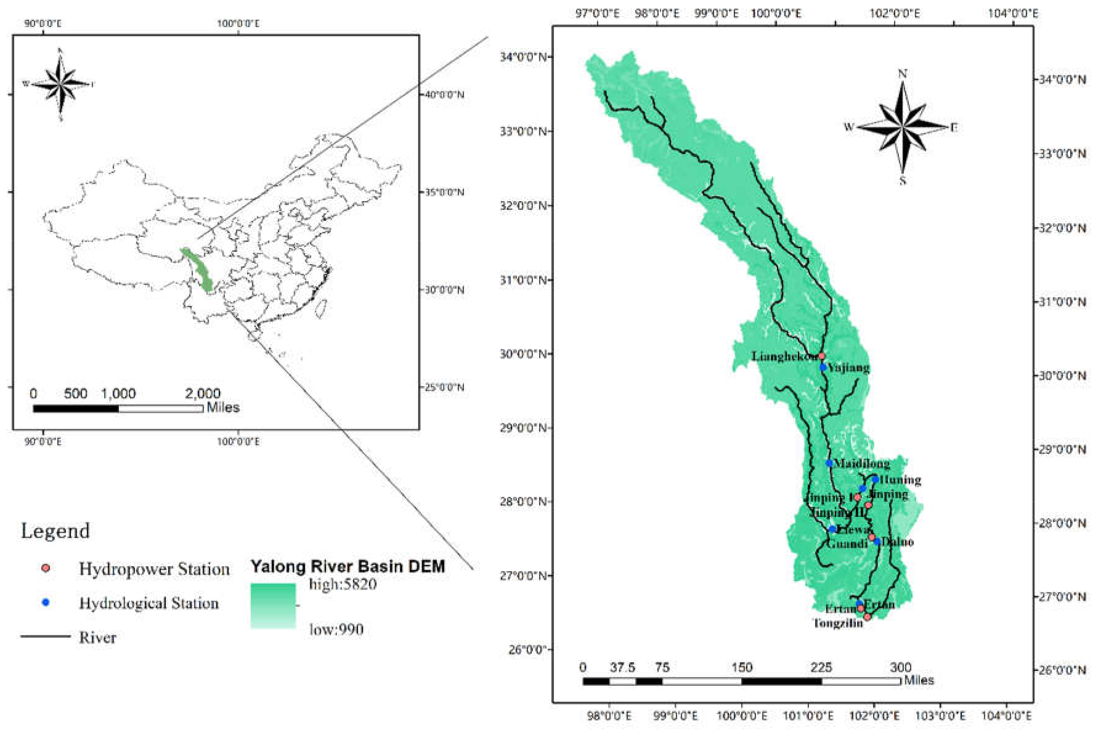
The Yalong River Basin is located in the eastern part of the Qinghai-Tibet Plateau, west of Sichuan Province, between Jinsha River and Dadu River. The geographical location is between 96°52′‒102°48′ E and 26°32′‒33°58′ N. Grassland covers approximately 51% of the catchment, and forest covers approximately 35% [27]. The total length of the main stream, which is the longest tributary of the Yangtze River, is about 1500 km, and the drainage area is about 130,000 km². There are many tributaries of the Yalong River, and the water system is well developed.

The Yalong River Basin belongs to the climatic region of the Western Sichuan Plateau, with a clear wet and dry season. The dry season is from November to April, and the rainy season is from May to October. The precipitation in the rainy season accounts for 90–95% of the annual precipitation, and rainy days account for about 80% of the whole year. The average annual precipitation in the Yalong River Basin is 500–2470 mm, and it has a growth trend from north to south. Watershed runoff is formed by precipitation, groundwater, and snowmelt (ice) water.

Due to the extremely rich water resources, the hydropower capacity in the Yalong River Basin is listed in the top ten in the country. Jinping I Hydropower Station, which started operation in 2013, has an installed capacity of 3600 MW, with an annual electricity production of 17.41 billion KW·h. The Ertan Hydropower Station started operation in 1998, with an installed capacity of 3300 MW and an annual electricity production of 17 billion KW·h. Guandi Hydropower Station started operation in 2012, with an installed capacity of 2400 MW and an average annual power generation of about 11.87 billion KW·h. Observation data for 2008–2011 are available for a total of 7 hydrological stations: Yajiang, Madilong, Liewa, Jinping, Huning, Daluo, and Ertan. The distributions of hydropower stations and hydrological stations are shown in Figure 1.

3. Data and Methods

3.1. Hydrological Model

The distributed watershed hydrological model is an important tool for simulating and analysing watershed hydrological processes. The SWAT (Soil and Water Assessment Tools) model is a typical semi-distributed hydrological model that can take natural factors, such as topography, climate, soil, land use, and land cover, into account, so that it has a strong physical foundation [28]. At present, many scholars have used this model to study the water quality of surface and underground runoff, sediment and nutrient transport, and point source and non-point source pollution [29,30,31]. This study uses the SWAT model at a daily scale to simulate the impact of reservoir operations on floods.

The SWAT model provides three methods to simulate the reservoir outflow [32]: (1) computing the outflow with an average annual release rate for an uncontrolled reservoir; (2) with pre-defined monthly/daily outflow; and (3) simulating the outflow with generalized operation rules based on the target reservoir storage. This study employs the third method, which simplifies the reservoir release process into two types: principal spillway and emergency spillway. Based on the corresponding reservoir storage of the two types of spillways, the target reservoir storage for the flood season and dry season is established. The advantage is that less data is required, and the high flow and low flow can be reasonably reconstructed.

For the target release approach, the principal spillway volume corresponds to the storage with a maximum flood control capacity, while the emergency spillway volume corresponds to the storage with no flood control capacity. In the non-flood season, the target storage is set at the emergency spillway volume. During the flood season, the flood control reservation for wet ground conditions is set at the maximum, and for dry ground conditions, it is set at 50% of the maximum. The target storage is calculated as [33]:

$$V_{t\arg }=V_{em} \mathrm{if} mo{n}_{fld,beg}<mon<mo{n}_{fld,end}$$

(1)

$$\begin{array}{c}{V}_{t\arg }=V_{pr}+\frac{(1-\min \left[\frac{SW}{FC},1\right])}{2}\cdot (V_{em}-V_{pr}) \mathrm{if}\\ mon\le mo{n}_{fld,beg} or mon\ge mo{n}_{fld,end}\end{array}$$

(2)

where $V_{t\arg }$ is the target reservoir storage for a given day (m³), $V_{em}$ is the storage of the reservoir when filled to the emergency spillway (m³), $V_{pr}$ is the storage of the reservoir when filled to the principal spillway (m³), $SW$ is the average soil water content in the sub-basin (m³), $FC$ is the water content of the sub-basin soil at field capacity (m³), $mon$ is the month of the year, $mo{n}_{fld,beg}$ is the first month of the flood season, and $mo{n}_{fld,end}$ is the last month of the flood season.

3.2. Data

The data used as inputs to the SWAT model include meteorology, a digital elevation model (DEM), and soil and land use datasets. Among these, the meteorological data are critical. The CMADS is a public dataset developed by Professor Xianyong Meng from China. The CMADS incorporates the technologies of LAPS (Local Analysis and Prediction System)/STMAS (Space-Time Multiscale Analysis System), and was constructed using multiple technologies and scientific methods, including loop nesting of data, projection of resampling models, and bilinear interpolation [34,35,36]. CMADS V1. 0 (spatial range 0°N to 65°N, 60°E to 160°E; spatial resolution 1/3°; temporal range 2008–2016) spatially divides the whole of East Asia into 300 × 195 grid points, a total of 58,500 sites; each site contains elements for daily average temperature, daily high/low temperature, daily precipitation, daily average solar radiation, daily average air pressure, daily specific humidity, and daily average wind speed [23,37].

Soil properties and land use types determine the runoff generation and confluence characteristics of different hydrological units, and they are also the basis for the definition of hydrological response units (HRU) in the SWAT model. The land use data (GLC2000 Data) is obtained from the Western China Environmental and Ecological Science Data Centre [38]. The soil data selected for this study is the China Soil Dataset, based on the Harmonized World Soil Database (HWSD) [39]. The Digital Elevation Model (DEM) is SRTM (Shuttle Radar Topography Mission) data, with a resolution of 90 m, from the International Scientific & Technical Data Mirror Site, Computer Network Information Centre, Chinese Academy of Sciences. A description of the data is given in

Table 1. A description of the data used for this study.

Dataset	Description of Dataset	Data Source	Time Scale
DEM	Shuttle Radar Topography Mission (SRTM) DEM 90M	http://www.gscloud.cn/	2007
Soil	China Soil Dataset based on the Harmonized World Soil Database (HWSD)	http://westdc.westgis.ac.cn	2009
Land use	European Union Joint Research Centre (JRC) Space Applications Institute (SAI) 2000 Global Land Cover Data Products (GLC2000)	http://westdc.westgis.ac.cn	2000
CMADS V1.0	Assimilation driving datasets applied to better reflect the spatial distribution of precipitation and meteorology	http://www.cmads.org	2008–2016

.

This paper is a study of the impact of reservoirs on runoff processes. Information on the reservoirs used in this study is shown in

Table 2. Information on the reservoirs used for this study.

Name	Start Year	Upper Water Level for Flood Control			Flood Control Level
		Water Level (m)	Volume (104 m3)	Area (ha)	Water Level (m)	Volume (108 m3)	Area (ha)
Guandi	2013	1330	72,920	1469	1328	70,070	1436
Jinping I	2012	1880	776,500	8255	1859.06	616,230	7064.9
Seasonal	2012	1838.09	479,334	6011.7	1827.06	416,038	5456.9

. Guandi is an annual regulation reservoir, with a regulation period of one year; the excess water in the wet season is stored to increase the water supply in the dry season. Jinping is a daily regulation reservoir, with a regulation period of one day; it regulates the water demand that varies within the course of a single day. This study required the establishment of a seasonal regulation reservoir to explore the impact of the storage capacity. The ratio of regulated storage capacity (V) to the annual average runoff (W) is the coefficient of storage (β). β of Jinping is 0.13 and β of Guandi is 0.0027. For a seasonal regulation reservoir, β is between 0.02 and 0.08; for this study, it was β = 0.05. Because we know the annual average runoff and β, we can calculate the regulated storage capacity, and then also calculate other factors. In the chart, we use “Seasonal” to represent a seasonal regulation reservoir created by a coefficient of storage.

3.3. Model Building

Based on watershed delineation, the basin is divided into 34 sub-basins and 694 hydrologic response units. The CMADS, soil, and land use were used as inputs to the model. Details of the input data for the SWAT model are shown in Table 1. The surface runoff is calculated by the SCS runoff curve method; the potential evapotranspiration is calculated by the Penman/Monteith method, and the flow concentration is calculated by the variable storage method.

With the construction and operation of the Ertan Hydropower Station in 1998, the basin above it remained a natural watershed. Therefore, the Ertan Hydropower Station was selected as the basin outlet. In all, seven observation stations were employed separately in the calibration, with one optimal parameter set obtained for each station. The observed flow for 2009–2011 (taking 2009 as a warm-up period) was used for calibration. Firstly, taking the sub-basins above the Yajiang station as a whole region, we used a set of parameters in this region. Adjusting this set of parameters enables the NSE (Nash-Sutcliffe Efficiency) and R² (Coefficient of Determination) to be optimized. Then, the set of optimal parameters was then brought back to the SWAT model. The same method was used to calibrate the next station, Maidilong. The calibration was not finished until the parameters of the outlet control station, Ertan, were determined. Then, the calibration parameters were used for model validation for 2008–2009 (taking 2008 as a warm-up period).

3.4. Sensitivity Analysis and Calibration Methodology

The physics of the SWAT model is controlled by multiple parameters, and each of them can affect the simulation results to some extent. Therefore, it is necessary to perform a parameter sensitivity analysis using the SWAT-CUP (SWAT Calibration and Uncertainty Programs) to improve the calculation efficiency and the accuracy of the simulation results [40].

SWAT-CUP is a computer program for the calibration of SWAT models, which links SUFI2 (Sequential Uncertainty Fitting Version 2), PSO (Particle Swarm Optimization), GLUE (Generalized Likelihood Uncertainty Estimation), ParaSol (Parameter Solution), and MCMC (Markov Chain Monte Carlo) procedures to the SWAT model. It enables sensitivity analysis, calibration, validation, and uncertainty analysis of SWAT models [41]. The SUFI-2 (Sequential Uncertainty Fitting ver. 2) algorithm has been widely used in model calibration and uncertainty analysis in recent years. Dao et al. [42] used four uncertainty algorithms to compare the runoff simulations of a SWAT model in a basin in Vietnam. The results show that SUFI-2 can obtain the best simulation results and uncertainty confidence intervals with the least number of simulations. In SUFI-2, parameter uncertainty accounts for all sources of uncertainties, such as the uncertainties in the driving variables (e.g., rainfall), conceptual model, parameters, and measured data [41]. The uncertainty is quantified by a measure referred to as the p-factor, which is the percentage of measured data bracketed by the 95% prediction uncertainty (95PPU). The 95PPU is calculated at the 2.5% and 97.5% levels of the cumulative distribution of an output variable obtained through Latin hypercube sampling [29].

3.5. Statistical Criteria for Evaluation

Different statistical criteria were used to evaluate the performance of the SWAT model during calibration and validation. According to Zhang et al. [43], the evaluation coefficients for runoff simulation effects include the coefficient of determination (R²) and the Nash-Sutcliffe efficiency (NSE).

R² is calculated as

$$R^2={\left[{\displaystyle \sum _i(Q_{obs}-\overline{Q_{obs}})(Q_{sim}-\overline{Q_{sim}})}\right]}^2{\displaystyle /}\left[{\displaystyle \sum _i{(Q_{obs}-\overline{Q_{obs}})}^2}\right]\left[{\displaystyle \sum _i{(Q_{sim}-\overline{Q_{sim}})}^2}\right]$$

(3)

where $Q_{obs}$ and $Q_{sim}$ represent the observed and simulated flow at Ertan, respectively. $\overline{Q_{obs}}$ is the mean of the observed flow for the entire time period of the evaluation, and $\overline{Q_{sim}}$ is the mean of the simulated flow for the entire time period of the evaluation. R² represents the proportion of the total variance in the observation data that can be explained by the model. R² ranges between 0.0 and 1.0, with higher values indicating a better performance [43].

NSE is calculated as

$$NSE=1.0-{\displaystyle \sum _i{(Q_{obs}-Q_{sim})}^2}/{\displaystyle \sum _i(Q_{obs}-\overline{Q_{obs}}}{)}^2$$

(4)

The meaning of the symbols is the same as above. The NSE indicates how well the observation values fit the simulated values, ranging from –∞ to 1 [44]. When the NSE is closer to 1, the simulation performance is better. A result of 1 means the observation values are completely consistent with the simulated values.

It is generally believed that a result of NSE > 0.5 and R² > 0.6 indicates a satisfactory performance [45]. According to the evaluation criteria of Moriasi [46], the NSE of the model is acceptable between 0.5 and 0.65, good between 0.65 and 0.75, and excellent between 0.75 and 1.0.

3.6. Scenarios

Both the capacity and operating location of the reservoir can have an impact on the downstream hydrological regime. Therefore, the runoff processes were simulated in eight scenarios (

Table 3. The scenarios for this study.

Scenario	Description	Objective	Reservoir capacity	Location
Scenario 1	Natural conditions	For comparison with other scenarios.	\	\
Scenario 2	One annual regulation reservoir	The impact of reservoir capacity on runoff.	Annual regulation reservoir	Sub-basin 19
Scenario 3	One annual regulation reservoir		Seasonal regulation reservoir	Sub-basin 19
Scenario 4	One daily regulation reservoir		Daily regulation reservoir	Sub-basin 19
Scenario 5	One annual regulation reservoir	The impact of reservoir location on runoff.	Annual regulation reservoir	Sub-basin 9
Scenario 6	One annual regulation reservoir		Annual regulation reservoir	Sub-basin 22
Scenario 7	Two reservoirs, with the annual regulation reservoir upstream	The impact of joint operation of reservoirs on runoff.	Annual regulation reservoir & daily regulation reservoir	Sub-basins 19 & 24
Scenario 8	Two reservoirs, with the daily regulation reservoir upstream		Daily regulation reservoir & annual regulation reservoir	Sub-basins 19 & 24

) with the reservoir added to the SWAT model with different capacities, operating locations (of a single reservoir), and relative locations (of two reservoirs). The simulations were then conducted by comparing the natural flow of the Ertan Control Station with the flow under different scenarios.

4. Results and Discussion

4.1. SWAT Calibration and Validation

According to the relevant literature on SWAT calibration and the characteristics of the Yalong River Basin, 17 sensitive parameters were selected for this study (shown in

Table 4. The calibrated parameter values selected for the SWAT model at Ertan station.

Parameter	Description	Type	Best Value	Sensitivity Ranking
CN2	SCS runoff curve number factor	r	0.06	1
ALPHA_BNK	Baseflow alpha factor for bank storage	v	0.84	2
CH_N2	Manning’s “n” value for the main channel	v	0.14	8
CH_K2	Effective hydraulic conductivity in main channel alluvium	v	304.5	12
ALPHA_BF	Baseflow alpha factor (days)	v	0.34	14
GW_DELAY	Groundwater delay (days)	v	270.5	6
GWQMN	Threshold depth of water in the shallow aquifer for "revap" to occur (mm)	v	50.81	7
REVAPMN	Threshold depth of water in the shallow aquifer for "revap" to occur (mm)	v	262.98	5
ESCO	Soil evaporation compensation factor	v	0.94	9
EPCO	Plant uptake compensation factor	v	0.12	3
SLSUBBSN	Average slope length	r	–0.25	4
SOL_AWC(1)	Available water capacity of the soil layer	r	3.23	13
SOL_K(1)	Saturated hydraulic conductivity	r	0.10	15
SOL_BD(1)	Moist bulk density	r	0.21	11
TLAPS	Temperature lapse rate	v	–4.42	10
SFTMP	Snowfall temperature	v	1.734	17
SMFMN	Minimum melt rate for snow during the year	v	10	16

). These 17 parameters were calibrated and validated using observation data from seven stations. The model calibration period was from 2009 to 2011, and 2009 was the model warm-up period. The model validation period was 2008 to 2009, and 2008 was the model warm-up period. Calibration efforts focused on improving the model performance at the main gauging stations. Since the basin upstream of Ertan Station is a natural watershed, Ertan Station is the focus of this study, and is used as an export control station. Table 4 shows the parameter sensitivity ranking and the optimum values of the station.

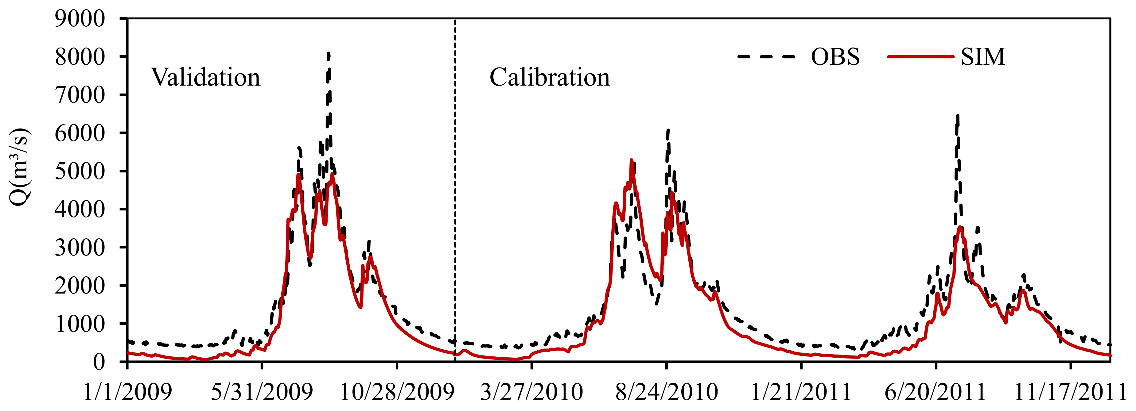
On the daily scale, the SWAT model simulation results achieved satisfactory results in seven control stations in the Yalong River basin (

Table 5. Evaluation indexes for the simulation result at the daily scale in Yalong River Basin.

Forcing Data	Indexes	Stations
		Yajiang	Maidilong	Liewa	Jinping	Huning	Daluo	Ertan
Calibration (2010–2011)	R²	0.84	0.84	0.78	0.85	0.85	0.85	0.87
	NSE	0.73	0.76	0.76	0.75	0.78	0.77	0.80
Validation (2009)	R²	0.85	0.86	0.80	0.90	0.91	0.92	0.93
	NSE	0.77	0.82	0.79	0.86	0.89	0.85	0.89

). For the model calibration period, the R² and NSE values of all stations were greater than 0.78 and 0.73, respectively. We also found that the model performance was better with the station further downstream. These evaluation criteria indicate that the results of the stations in the Yalong River Basin are very good on the daily scale. For the validation period, the R² value of each station in the basin was greater than 0.8, and even reached 0.9 for Jinping, Huning, and Ertan. The NSE of each station was greater than 0.77, which indicates that the runoff simulation results in the Yalong River basin were in good agreement with the daily observation values. To sum up, this model is applicable to the Yalong River basin. The results of the runoff at the Ertan station during the calibration and validation period are shown in Figure 2. It can be seen from the figure that the simulation is generally consistent with the observations, and the performance of the SWAT model is satisfactory.

4.2. The Impact of Reservoir Capacity on Runoff

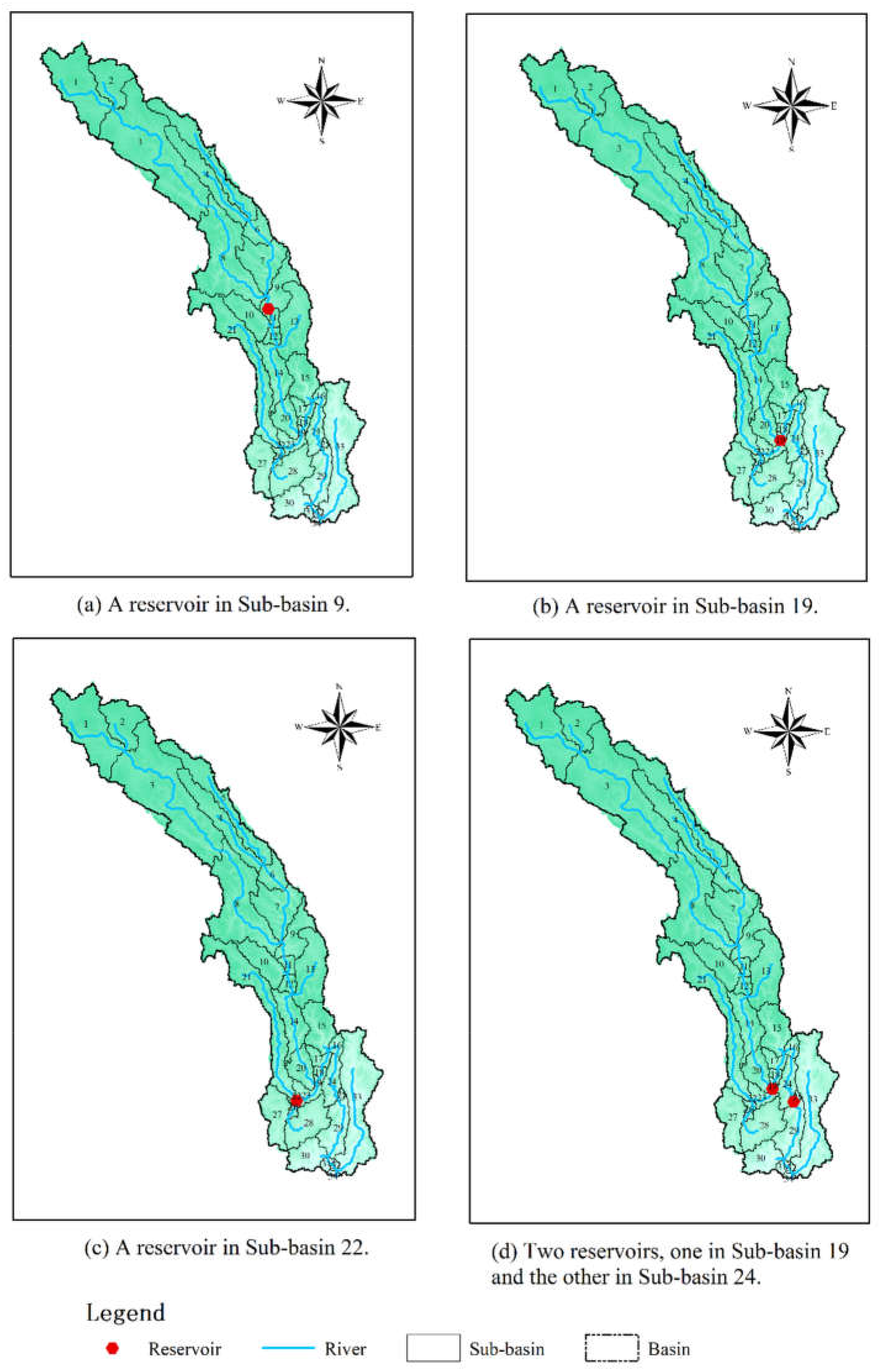
Four scenarios (Scenarios 1, 2, 3, and 4) are considered in this section. The parameters of the reservoirs are shown in Table 2, and the location information is shown in Figure 3(a).

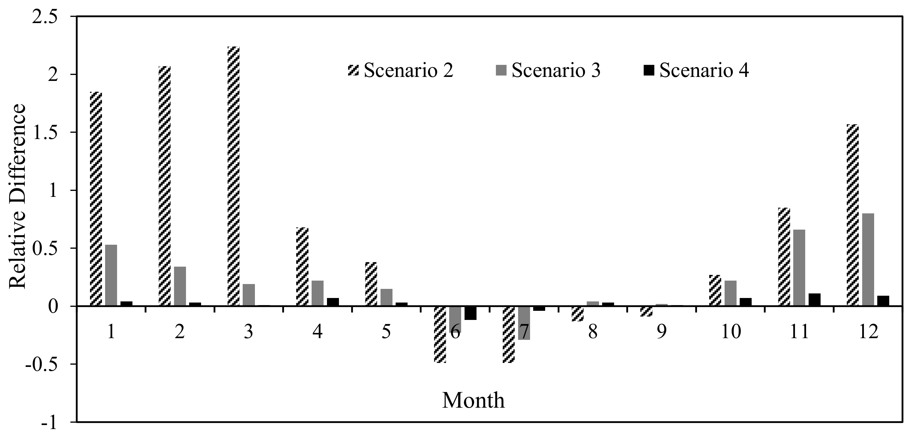
Figure 4 shows the relative difference of the annual, seasonal, and daily regulation reservoir on the monthly average flow (2009–2016) at the Ertan control station. The relative difference is calculated as the ratio of the difference between the average monthly flow with a reservoir and without a reservoir, and the monthly average flow without a reservoir. It can be seen from Figure 4 that the average monthly flow with the reservoir is significantly increased compared to the natural monthly average flow in the dry season from October to May, with the most noticeable increase occurring between January and March. Furthermore, a larger increase in dry season runoff can be observed with increasing capacity. The annual regulation reservoir has the greatest increment in the monthly average flow in the dry season. During the flood season, from June to September, the annual regulation reservoir exhibits a strong ability to mitigate floods, especially in the early flood season. The seasonal regulation reservoir and the daily regulation reservoir result in a decrease in runoff from June to July, and a slight increase from August to September. Due to its limited storage capacity, the small reservoir will increase the release rate to ensure its safety in the case of a major flood.

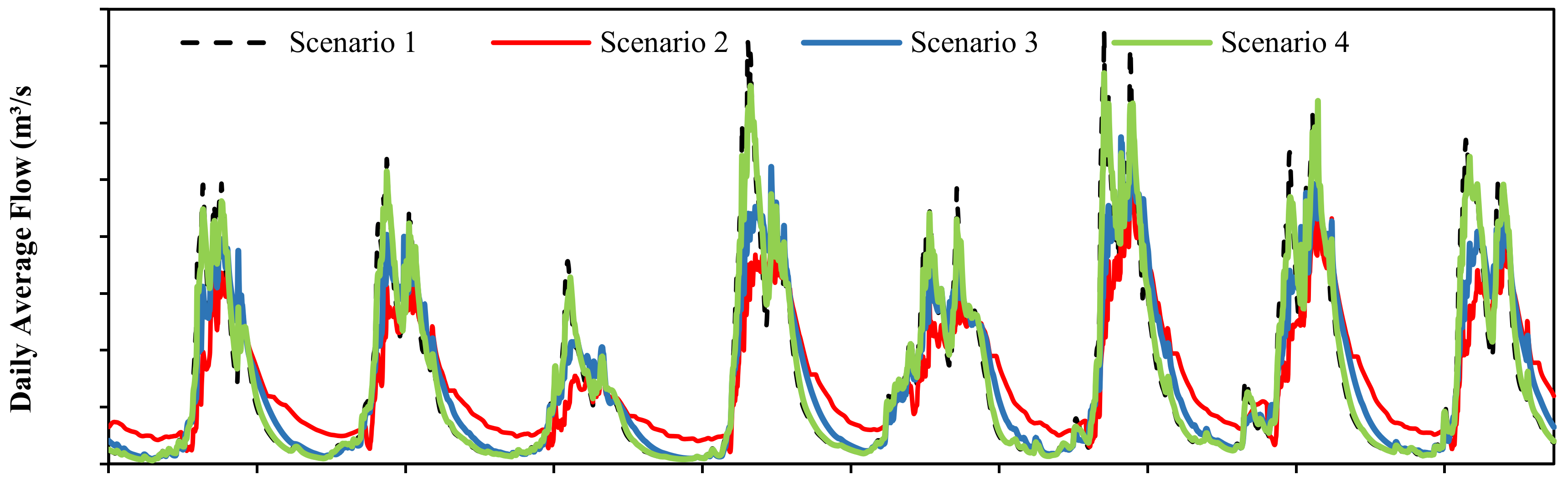
Figure 5 is a simulation result of the daily runoff at Ertan control station under four scenarios. The figure illustrates that the reservoir reduces the flood during the flood season, while it supplies more water during the dry season. The annual regulation reservoir mitigates the flood peak flow the most, and largely weakens the flood peak in the early flood season. Double peak or multi-peak phenomena are most common in the Yalong River Basin. If there is heavy rainfall at the end of the flood season, the reservoir’s mitigation of the flood will be decreased due to it having filled earlier in the flood season. The effect of the seasonal regulation reservoir on the peak flow during the flood season is less than that of the annual regulation reservoir, while the daily regulation reservoir has the least impact on the flood. During the dry season, the annual regulation reservoir has the greatest runoff recharge. The seasonal regulation reservoir is slightly inferior, while the daily regulation reservoir is the worst.

In this study, the annual maximum peak flow, peak time, and maximum three-day flood volume were used to evaluate the impact of the reservoir operation on runoff (details in

Table 6. Flood characteristics analysis at Ertan station (Scenarios 1–4). (Q_max represents annual maximum peak flow, T_Qmax represents peak time, and W_3,day represents maximum three-day flood volume.).

Index	Scenario	Year	2009	2010	2011	2012	2013	2014	2015	2016
Qmax (m3/s)	1	Value	4929	5353	3565	7419	4832	7616	6200	5701
	2	Relative Difference (%)	−28.9	−29.1	−48.9	−33.8	−30.4	−34.3	−16.8	−31.1
	3	Relative Difference (%)	−18.5	−24	−39.1	−30	−21	−25	−6.6	−25
	4	Relative Difference (%)	−6.2	−4	−8.1	−10.3	−8.8	−9.7	3	−5.2
TQmax	1	Value	2009/8/17	2010/7/17	2011/7/18	2012/7/16	2013/9/11	2014/7/6	2015/9/5	2016/7/6
	2	Difference (d)	34	45	70	47	0	34	6	76
	3	Difference (d)	−17	45	18	47	0	34	6	76
	4	Difference (d)	0	0	5	5	−55	0	6	8
W3,day (108m3)	1		17.8	19.1	13	26.8	17.1	26.2	21.8	20.7
	2	Relative Difference (%)	−31.5	−31.9	−49.2	−36.9	−33.3	−31.7	−24.8	−31.4
	3	Relative Difference (%)	−18.5	−25.1	−38.5	−32.5	−23.4	−22.1	−14.7	−25.1
	4	Relative Difference (%)	−5.1	−3.7	−10	−10.1	−10.5	−11.1	−3.7	−6.8

). As shown in Table 6, the annual regulation reservoir reduces the annual maximum peak flow by 28–48.9% (2011). The maximum reduction of peak flow by the seasonal regulation reservoir is 39.8% (2011), but in the remaining years, the reduction is below 30%. The reduction of the peak flow by the daily regulation reservoir is less than 10%. In the natural scenario, without a reservoir, the annual maximum flow is mainly concentrated between July and August. After regulation by the annual regulation reservoir, the annual maximum flow is basically delayed to September, by more than 30 days (except in 2013 and 2015). The seasonal regulation reservoir has a similar effect to the annual regulation reservoir. The daily regulation reservoir delays the peak flow by less than 8 days, except in 2013, in which it is delayed by 55 days. In the scenarios with reservoirs, the annual maximum three-day flood volume is reduced to varying degrees. Compared with the natural situation, the maximum three-day flood volume in Scenario 2 has been reduced by 24.8–49.8%; in Scenario 3, it is reduced by 14.7–38.5%, and in Scenario 4, it is reduced by less than 11.1%.

Table 6 shows that for scenarios with reservoirs, the reduction of the peak flow and the maximum three-day flood volume was greatest during 2012–2014, and smallest in 2015. This indicates that the reservoir has a stronger mitigation effect on larger flood volumes. The smallest reduction in 2015 may be due to a major flood in 2014, which could still impact the following year, resulting in a decreased ability of the reservoirs to control flooding.

4.3. The Impact of Reservoir Location on Runoff

Four scenarios are considered in this section, including Scenarios 1, 2, and 5 (Figure 3b), and Scenario 6 (Figure 3c). The parameters of the reservoirs are shown in Table 2.

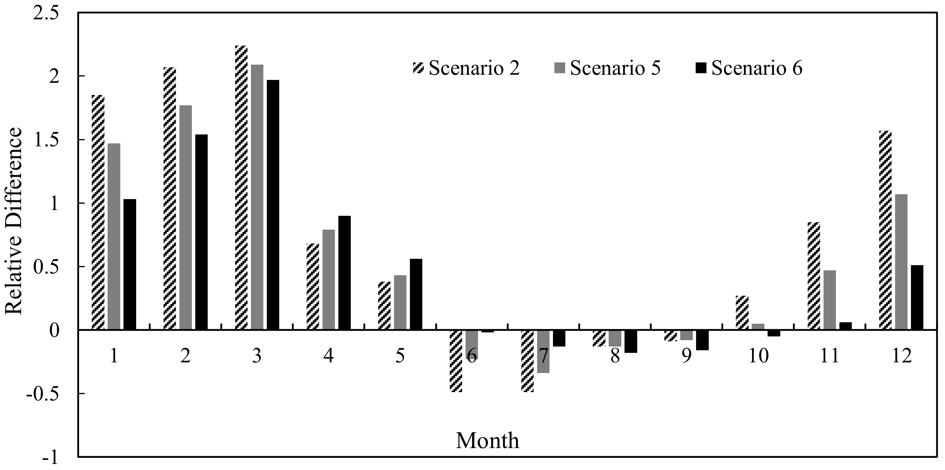
Figure 6 shows the relative difference in the monthly average flow (2009–2016) at the Ertan control station depending on whether the annual regulation reservoir is in Sub-basin 19, 9, or 22, or under natural conditions without a reservoir. The relative difference is calculated as above. It can be concluded from Figure 6 that the hydrograph of Scenario 2 becomes flattened compared with the natural situation, and changes even more. On the other hand, the hydrograph experiences only a minor change under Scenario 6.

The average monthly flow under Scenarios 2, 5, and 6 is increased compared with the natural average monthly flow in the dry season (except for the reservoir located in Sub-basin 22 in October). The monthly average flow from December to March changes more and increases month by month. Furthermore, the replenishment effect on runoff in the dry season is enhanced when the reservoir is downstream of the main stream, and is lowest when the reservoir is located in the tributary (Sub-basin 22). Due to small floods in 2013 and 2015, the average monthly flow was larger than usual from April to May. The reservoir located upstream (Sub-basin 19) and in a tributary (Sub-basin 22) had little regulating effect on the runoff. The monthly average flow from April to May therefore differs as follows: Scenario 6 > Scenario 5 > Scenario 2.

During the flood season, Scenario 2 has a greater capacity to impound floods than Scenarios 5 or 6, indicating that a reservoir located downstream of the main stream is best for mitigating floods. In August–September, Scenario 6 is better than Scenarios 2 or 5 in impounding floods. This may be due to the large amount of water stored in the reservoirs during the first flood in Scenario 2 and Scenario 5. When the second flood occurs in the basin, although its peak flow is lower than the first one, the remaining reservoir capacity is smaller. Therefore, the capacity to impound water is limited, and the reduction of the flood peak flow is weakened.

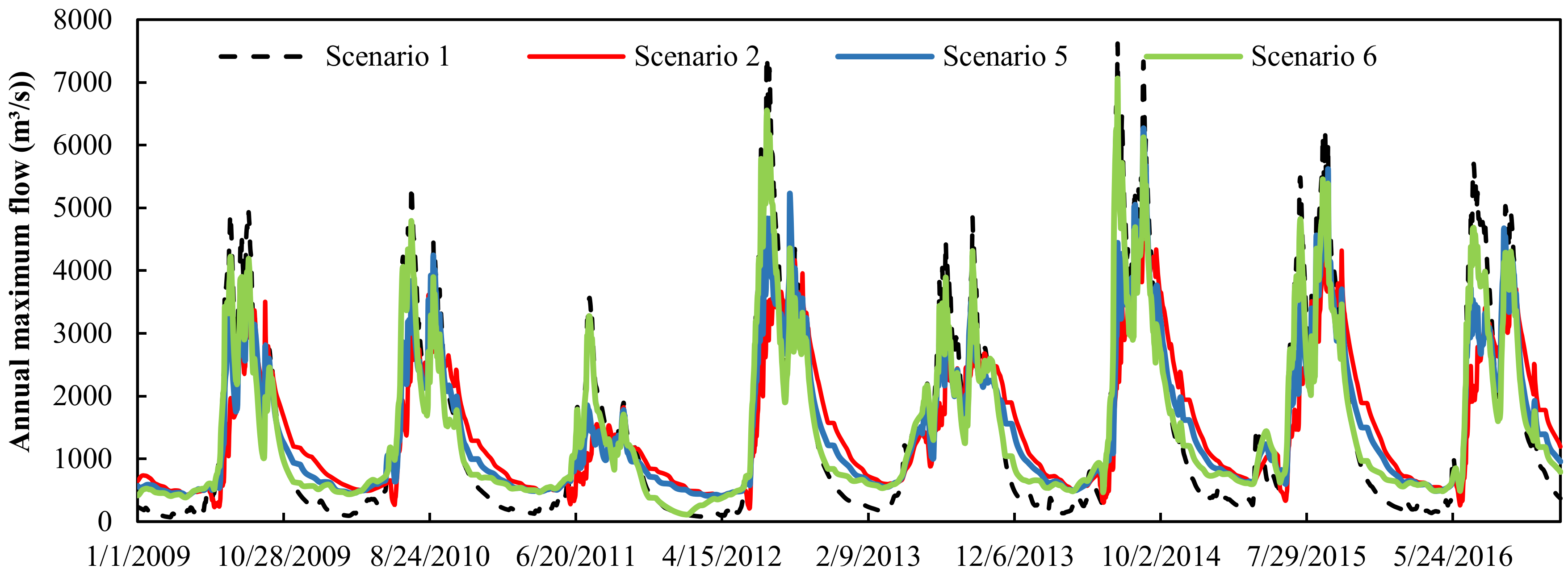
Figure 7 is a simulation result of the daily runoff at Ertan control station under Scenarios 1, 2, 5, and 6. It is most obvious that a reservoir reduces the flood peak flow, and increases runoff in the dry season, in scenario 2. The effect of Scenario 5 is the second greatest, while the effect of Scenario 6 is the smallest. It illustrates that a reservoir located downstream of the main stream has a better regulation effect on the runoff, when the reservoir capacity is the same.

The annual maximum peak flow, peak time, and maximum three-day flood volume under Scenarios 1, 2, 5, and 6 are shown in

Table 7. Flood characteristics analysis at Ertan station (Scenarios 1–2 & 5–6). (Q_max represents annual maximum peak flow, T_Qmax represents peak time, and W_3,day represents maximum three-day flood volume.).

Index	Scenario	Year	2009	2010	2011	2012	2013	2014	2015	2016
Qmax (m3/s)	1	Value	4929	5353	3565	7419	4832	7616	6200	5701
	2	Relative Difference (%)	−28.9	−29.1	−48.9	−33.8	−30.4	−34.3	−16.8	−31.1
	5	Relative Difference (%)	−22.6	−21.1	−48	−29.7	−12.4	−17.8	−9.4	−18.2
	6	Relative Difference (%)	−14.3	−10.8	−8.1	−11.7	−11.1	−7.3	−12.1	−17.9
Time (Qmax)	1	Value	2009/8/17	2010/7/17	2011/7/18	2012/7/16	2013/9/11	2014/7/6	2015/9/5	2016/7/6
	2	Difference (d)	34	45	70	47	0	34	6	76
	5	Difference (d)	−16	45	−5	47	0	53	6	62
	6	Difference (d)	−37	0	−1	0	0	0	−5	0
W3,day (108m3)	1		17.8	19.1	13	26.8	17.1	26.2	21.8	20.7
	2	Relative Difference (%)	−31.5	−31.9	−49.2	−36.9	−33.3	−31.7	−24.8	−31.4
	5	Relative Difference (%)	−23	−22	−48.5	−31	−15.2	−14.1	−12.8	−19.8
	6	Relative Difference (%)	−14	−11.5	−8.5	−11.6	−11.7	−8.8	−12.8	−16.9

; the annual regulation reservoir in sub-basin 19 reduces the annual maximum peak flow from 16.8% to 48.9%. The absolute value of the annual maximum flow change in Scenario 5 (sub-basin 9) is 0.9–18% lower than that in Scenario 2 (sub-basin 19). When the reservoir is located in the tributary (sub-basin 22), the maximum peak flow is reduced by 7.3–17.9% compared with the natural situation. In this scenario, the change in annual maximum flow is the smallest.

In Scenario 5, the annual maximum peak flow in 2009 and 2011 appeared earlier than in the natural situation. In 2014, the peak flow occurred 19 days later than in Scenario 2. In 2010, 2012, and 2013, it was the same as in Scenario 2. In Scenario 6, the annual maximum peak flow in 2009, 2011, and 2015 appeared earlier than in the natural situation, and in the other years, it was the same as the natural situation. In Scenarios 2, 5, and 6, the annual maximum three-day flood volume was reduced to varying degrees. The absolute change in the annual maximum three-day flood volume under Scenario 5 was 0.8–18.1% smaller than under Scenario 2. The annual maximum three-day volume in Scenario 6 was 8.5–16.9% lower than in the natural situation.

Table 7 shows that a reservoir located in the mainstream (Scenarios 2 and 5) has a stronger decreasing effect on a large flood. When the reservoir is on the tributary (Scenario 6), the flood reduction is better for medium floods.

4.4. The Impact of Joint Operation of Dual Reservoirs on Runoff

The four Scenarios considered in this section are Scenarios 1, 2, 7, and 8 (Figure 3d). The parameters of the reservoirs are shown in Table 2.

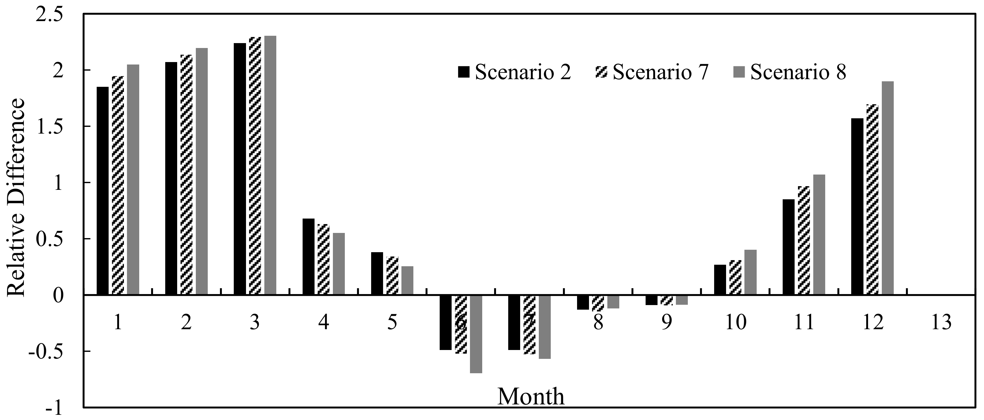
Figure 8 shows the relative differences of monthly average flow (2009–2016) when Scenarios 2, 7, and 8 are compared with the natural conditions. As can be seen from Figures 10 and 11, the flow curves of Scenario 2 and Scenario 7 are very close. Adjusting the relative location of the two reservoirs results in a small change in runoff, and both Scenarios make the monthly average flow curve flatter. Scenario 8 has a greater impact on flood mitigation during the early flood season (June–July), but a lower impact than Scenario 7 later in the flood season.

In general, when the small reservoir is located upstream of the large reservoir, the reduction of the flood is greater in the flood season, and the increase in runoff is greater in the dry season. When the large reservoir is located upstream of the small reservoir, the runoff regulation of the large reservoir will be affected by the downstream small reservoir, which will weaken the overall performance of the joint operation of the reservoirs. Mainly because of the limited capacity of small reservoirs and the poor performance of runoff regulation, the large reservoir should decreased the release in case of a break of the dams.

When the basin contains only an annual regulation reservoir, the runoff regulation is minimal. However, the difference is small under Scenario 2 and 7. This means that there is little advantage in placing the small reservoir downstream of the large reservoir to improve their overall regulation capacity.

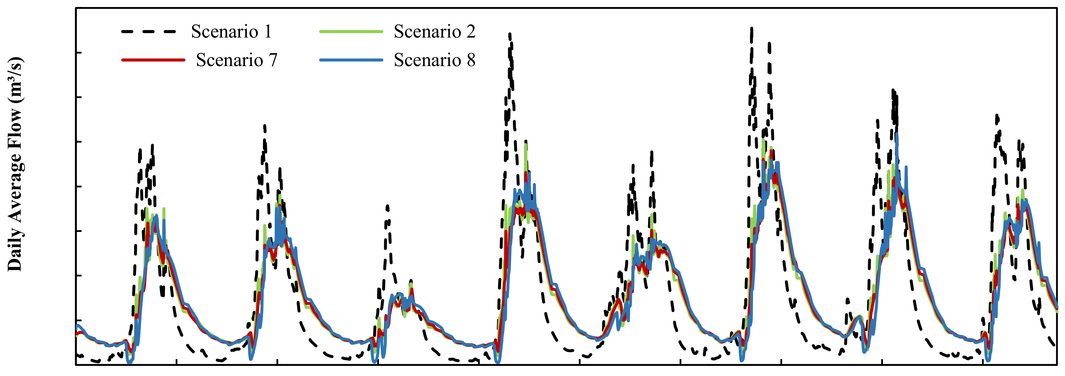
Figure 9 shows the daily runoff simulation at Ertan control station under Scenarios 1, 2, 7 & 8. The three Scenarios with reservoirs are essentially the same. However, the runoff in Scenario 2 fluctuates greatly and the flood peak is higher. The increase in runoff during the water supply period differs as follows: Scenario 8 > Scenario 7 > Scenario 2.

The annual maximum peak flow, peak time, and maximum three-day flood volume under Scenarios 1, 7, and 8 are shown in

Table 8. Flood characteristics analysis at Ertan station (Scenarios 1 & 7–8). (Q_max represents annual maximum peak flow, T_Qmax represents peak time, and W_3,day represents maximum three-day flood volume.).

Index	Scenario	Year	2009	2010	2011	2012	2013	2014	2015	2016
Qmax (m3/s)	1	Value	4929	5353	3565	7419	4832	7616	6200	5701
	7	Relative Difference (%)	−35.2	−33.3	−52.3	−42.1	−37.6	−37	−16.8	−36.5
	8	Relative Difference (%)	−32.1	−34	−55	−42.4	−41.6	−39.7	−16.5	−35.3
Time (Qmax)	1		2009/8/17	2010/7/17	2011/7/18	2012/7/16	2013/9/11	2014/7/6	2015/9/5	2016/7/6
	7	Difference (d)	5	45	72	47	0	58	6	74
	8	Difference (d)	12	45	36	57	0	58	6	87
W3,day (108m3)	1		17.8	19.1	13	26.8	17.1	26.2	21.8	20.7
	7	Relative Difference (%)	−34.8	−36.6	−53.1	−43.3	−39.2	−35.5	−25.2	−36.2
	8	Relative Difference (%)	−31.5	−40.3	−54.6	−44.8	−40.9	−37	−24.3	−35.3

. In 2011, the relative difference of the annual maximum flow in Scenarios 7 and 8 reached the maximums at the same time, with values of 52.3% and 55%, respectively. In 2015, they reached the minimum values, which were 16.8% and 16.5%, respectively. It can be seen that the change of the annual maximum flow is not much different in the two Scenarios. The differences between the absolute values of the maximum three-day flood volume fluctuate within 4% in the two scenarios. In combination with Table 7, the decrease in the annual maximum flow and maximum three-day flood volume in Scenarios 7 and 8 is higher than that in Scenario 2, except in 2015.

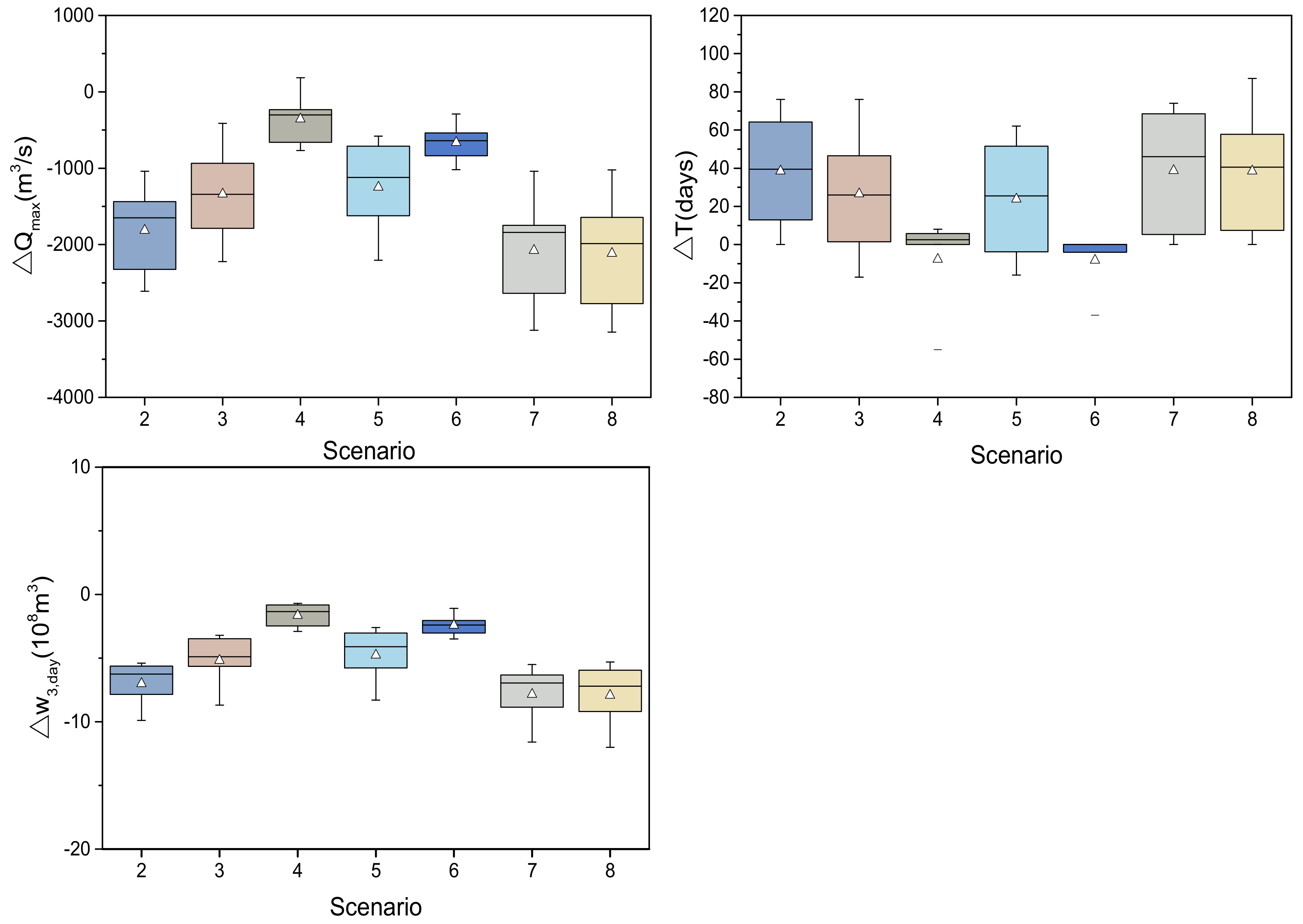
In order to clearly show the difference between the seven scenarios with reservoirs, relative to the natural conditions (i.e., the annual maximum flow, peak time, and maximum three-day flood volume distribution and median), a box-line diagram is used to compare the impacts of the reservoir on the runoff processes in all scenarios (Figure 10). For the change in flood peak flow, the medians of Scenarios 7 and 8 are close, and their absolute values are the largest, while the median absolute value of Scenario 4 is the smallest. This shows that the scenarios with two reservoirs have a greater ability to regulate runoff, and the scenario with a daily regulation reservoir has the least ability to regulate runoff, followed by Scenario 6. This means that when the reservoir is located in the tributary, it will greatly weaken its ability to regulate runoff. The median number of days by which the annual maximum flow is delayed under Scenarios 4 and 6 are close, and the range is narrow and concentrated around 0. Other scenarios make little difference in delaying the annual maximum flow. For the reduction of the maximum three-day flood volume, the absolute value of the median becomes smaller as the reservoir capacity decreases.

It can also be seen from Figure 13 that as the reservoir capacity decreases, the absolute value of the median of all flood characteristic values becomes smaller, and the reservoir regulation capacity becomes lower. The medians and ranges under Scenario 2 and Scenario 5 are relatively close, indicating that the regulation capacity of the seasonal regulation reservoir downstream is similar to that of the annual regulation reservoir upstream in the Yalong River Basin. The medians and ranges under Scenario 4 and Scenario 6 are relatively close, indicating that the regulation capacity of the daily regulation reservoir downstream in the Yalong River Basin is similar to that of the annual regulation reservoir upstream in the tributary. The medians and ranges of Scenario 7 and Scenario 8 are close, which indicates that the relative location of the large reservoir and the small reservoir has little effect on their joint operation, but Scenario 8 is better.

5. Conclusions

Reservoirs are often designed for multiple objectives, such as hydropower generation, flood control, and water supply, and they are operated in such a way that the water can be spatially and temporally redistributed for the benefit of the water users. Obviously, the impact of reservoirs on runoff, especially during floods, is directly correlated to their capacity, location, and joint operation. This study therefore aimes to quantitatively assess the potential impact of different reservoir configurations on the runoff, by changing the capacity and location of a single reservoir, and the relative location of dual reservoirs.

With respect to the influence of the storage capacity on runoff, it was found that the storage capacity is generally in proportion to the effect on runoff regulation, regardless of flood seasons and non-flood seasons. The annual regulation reservoir performs better at reducing the flood peak flow and delaying the flood peak appearance time. Due to a limited storage capacity, the small reservoir may increase its water release in the event of a large flood to ensure dam safety. Therefore, for areas with abundant water resources, like Yalong River Basin, we recommend the construction of large reservoirs if the geographical and economic conditions permit, as this is beneficial to the improvement of flood control in the basin.

As for the influence of the reservoir’s location on runoff, it was found that the reservoir in the main stream shows greater regulation capability than the reservoir in the tributary. The regulation capability increases when the reservoir is further downstream, and decreases when the reservoir is further upstream. Therefore, we recommend constructing the reservoir downstream from the mainstream of Yalong River, so that it can play a more vital role in flood control.

An analysis of the influence on runoff of the relative locations of two reservoirs indicates that locating the daily regulation reservoir upstream of the annual regulation reservoir is beneficial to flood control. However, the relative location of two reservoirs makes little difference to the impact on runoff. Runoff regulation capability is generally greater as the number of reservoirs increases. Therefore, building small reservoirs downstream from large reservoirs in the Yalong River Basin is not recommended, as it is not conducive to flood control.

Overall, reservoir operation can mitigate floods and delay the flood peak appearance time in the flood season, and it can release more water to meet downstream water demands in the dry season. Runoff processes tend to become flattened. Moreover, reservoirs can have a more significant effect on relatively large floods. Therefore, in areas similar to Yalong River Basin, where the annual distribution of runoff is uneven, we recommend building cascade reservoirs to regulate the annual distribution of runoff, and to achieve rational water resources management.

References

- Zhang, R.; Zhang, T.; Pei, W. Flood Analysis of Fengshuba Reservoir Considering the Influence of upstream hydraulic engineering. China R. Water Hydropower 2008, 8, 29–31. [Google Scholar]
- Hu, Q.; Yin, T. Impact assessment of climate change and human activities on annual highest water level of Taihu Lake. Water Sci. Eng. 2009, 2, 1–15. [Google Scholar]
- International Commission of Large Dams (ICOLD). World Register of Dams; Int. Comm. Large Dams: Paris, France, 2007. [Google Scholar]
- World Commission on Dams (WCD). Dams and Development: A New Framework for Decision-Making; World Commission on Dams (WCD): London, UK, 2000. [Google Scholar]
- Wan, X.; Guan, X.; Zhong, P.; Wang, M.; Mei, J. Impact of large-scale multiple reservoir on basin flood hydrograph. Adv. Sci. Technol. Water Resources 2017, 3, 66–71. [Google Scholar]
- Assani, A.A.; Landry, R.; Daigle, J. Alain, Chalifour. Reservoirs Effects on the Interannual Variability of Winter and Spring Streamflow in the St-Maurice River Watershed (Quebec, Canada). Water Resources Manag. 2011, 25, 3661–3675. [Google Scholar] [CrossRef]
- Vicente-Serrano, S.M.; Zabalza-Martínez, J.; Borràs, G.; López-Moreno, J.I.; Pla, E.; Pascual, D.; Savé, R.; Biel, C.; Funes, I.; Martín-Hernández, N.; et al. Effect of reservoirs on streamflow and river regimes in a heavily regulated river basin of Northeast Spain. Catena 2017, 149, 727–741. [Google Scholar] [CrossRef] [Green Version]
- Moyle, P.B.; Mount, J.F. Homogenous rivers, homogenous faunas. Proc. Natl. Acad. Sci. USA 2007, 104, 5711–5712. [Google Scholar] [CrossRef] [Green Version]
- Döll, P.; Fiedler, K.; Zhang, J. Global-scale analysis of river flow alterations due to water withdrawals and reservoirs. Hydrol. Earth Syst. Sci. 2009, 13, 2413–2432. [Google Scholar] [CrossRef] [Green Version]
- Aus der Beek, T.; Flörke, M.; Lapola, D.M.; Schaldach, R.; Voß, F.; Teichert, E. Modelling historical and current irrigation water demand on the continental scale: Europe. Adv. Geosci. 2010, 27, 79–85. [Google Scholar] [CrossRef] [Green Version]
- Dou, Y.; Yang, W. Effect of Water Resource Projects along Caoe River Basin on Ecological Environments. Adv. Water Sci. 1996, 7, 260–267. [Google Scholar]
- Biemans, H.; Haddeland, I.; Kabat, P.; Ludwig, F.; Hutjes, R.W.A.; Heinke, J.; von Bloh, W.; Gerten, D. Impact of reservoirs on river discharge and irrigation water supply during the 20th century. Water Resour. Res. 2011, 47, 77–79. [Google Scholar] [CrossRef]
- Li, C.; Xue, Z.; Peng, Y.; Zhou, H.; Liu, Y. Impacts of Hydraulic Engineering on Flood. South-to-North Water Transfers Water Sci. Technol. 2014, 12, 21–25. [Google Scholar]
- Zhang, Z.; Zhang, Q.; Deng, X.; Liu, J.; Sun, P. Hydrological Effects of Water Reservoirs on Fluvial Hydrological Process for the East River Basin Using Statistical Modeling Technique. J. Nat. Resour. 2015, 30, 684–695. [Google Scholar]
- Yigzaw, W.; Hossain, F.; Kalyanapu, A. Impact of Artificial Reservoir Size and Land Use/Land Cover Patterns on Probable Maximum Precipitation and Flood: Case of Folsom Dam on the American River. J. Hydrol. Eng. 2013, 18, 1180–1190. [Google Scholar] [CrossRef]
- Chen, T.; Dong, Z.; Jia, B.; Huang, X.; Zhong, D. Analysis of design flood of dam site of Xiaonanhai Hydropower Station considering flood control operation of upstream cascade reservoir group. J. Hohai Univ. (Nat. Sci.) 2014, 42, 476–480. [Google Scholar]
- Yang, D.; Ye, B.; Kane, D.L. Streamflow changes over Siberian Yenisei River Basin. J. Hydrol. (Amsterdam) 2004, 296, 59–80. [Google Scholar] [CrossRef]
- Liu, J.; Shanguan, D.; Liu, S.; Ding, Y. Evaluation and Hydrological Simulation of CMADS and CFSR Reanalysis Datasets in the Qinghai-Tibet Plateau. Water 2018, 10, 513. [Google Scholar] [CrossRef]
- Meng, X.; Wang, H.; Cai, S.; Zhang, X.; Leng, G.; Lei, X.; Shi, C.; Liu, S.; Shang, Y. The China Meteorological Assimilation Driving Datasets for the SWAT Model (CMADS) Application in China: A Case Study in Heihe River Basin. Preprint 2016. [Google Scholar] [CrossRef]
- Dong, N.; Yang, M.; Meng, X.; Liu, X.; Wang, Z.; Wang, H.; Yang, C. CMADS-Driven Simulation and Analysis of Reservoir Impacts on the Streamflow with a Simple Statistical Approach. Water 2018, 11, 178. [Google Scholar] [CrossRef]
- Meng, X.; Wang, H.; Lei, X.; Cai, S.; Wu, H. Hydrological Modeling in the Manas River Basin Using Soil and Water Assessment Tool Driven by CMADS. Tehnički Vjesnik 2017, 24, 525–534. [Google Scholar]
- Meng, X.; Dan, L.; Liu, Z. Energy balance-based SWAT model to simulate the mountain snowmelt and runoff – taking the application in Juntanghu watershed (China) as an example. J. Mt. Sci. 2015, 12, 368–381. [Google Scholar] [CrossRef]
- Wang, Y.; Meng, X. Snowmelt runoff analysis under generated climate change scenarios for the Juntanghu River basin in Xinjiang, China. Tecnología y Ciencias del Agua 2016, 7, 41–54. [Google Scholar]
- Meng, X. Simulation and spatiotemporal pattern of air temperature and precipitation in Eastern Central Asia using RegCM. Sci. Rep. 2018, 8, 3639. [Google Scholar] [CrossRef] [Green Version]
- Du, J.; Zhou, G. A Recursive Optimal Algorithm for the Operation of Multireservoir Flood Control System. Adv. Water Sci. 1994, 5, 134–141. [Google Scholar]
- Mei, Y.; Yang, N.; Yan, L. Optimal ecological sound operation of cascade reservoirs in the lower Yalongjiang River. Adv. Water Sci. 2009, 20, 721–725. [Google Scholar]
- Yu, X.; Feng, L.; Yan, D.; Jia, Y.; Yang, S.; Hu, D.; Zhang, M. Development of distributed hydrological model for Yalongjiang River basin. China Hydrol. 2008, 28, 49–53, (In Chinese with English abstract). [Google Scholar]
- Arnold, J.G.; Srinivasan, R.; Muttiah, R.S.; Williams, J.R. Large area hydrologic modeling and assessment part I: Model development. J. Am. Water Resour. Assoc. 1998, 34, 73–89. [Google Scholar] [CrossRef]
- Abbaspour, K.C.; Yang, J.; Maximov, I.; Maximov, I.; Siber, R.; Bogner, K.; Mieleitner, J.; Zobrist, J.; Srinivasan, R. Modelling hydrology and water quality in the pre-alpine/alpine Thur watershed using SWAT. J. Hydrol. 2007, 333, 413–430. [Google Scholar] [CrossRef]
- Chaplot, V. Impact of DEM mesh size and soil map scale on SWAT runoff, sediment, and NO 3 –N loads predictions. J. Hydrol. 2005, 312, 207–222. [Google Scholar] [CrossRef]
- Jayakrishnan, R.; Srinivasan, R.; Santhi, C.; Arnold, J. Advances in the application of the SWAT model for water resources management. Hydrol. Processes 2005, 19, 749–762. [Google Scholar] [CrossRef]
- Li, W.; Chen, X.; He, Y.; Zhang, L. Modification of Reservoir Module in SWAT model and its Application of Runoff Simulation in Highly Regulated Basin. Trop. Geol. 2018, 38, 226–265. [Google Scholar]
- Neitsch, S.L.; Arnold, J.G.; Kiniry, J.R.; Williams, J.R. Soil and Water Assessment Tool Theoretical Documentation Version 2009; TWRI Report TR-191; Texas Water Resources Institute: College Station, TX, USA, 2011; pp. 416–422. [Google Scholar]
- Meng, X. Spring Flood Forecasting Based on the WRF-TSRM mode. VJESN 2018, 25, 27–37. [Google Scholar]
- Meng, X.; Wang, H.; et al. Investigating spatiotemporal changes of the land-surface processes in Xinjiang using high-resolution CLM3.5 and CLDAS: Soil temperature. Sci. Rep. 2017, 7, 13286. [Google Scholar] [CrossRef] [PubMed] [Green Version]
- Meng, X.; Wang, H. Significance of the China Meteorological Assimilation Driving Datasets for the SWAT Model (CMADS) of East Asia. Water 2017, 9, 765. [Google Scholar] [CrossRef]
- Meng, X.; Wang, H.; Shi, C.; Wu, Y.; Ji, X. Establishment and Evaluation of the China Meteorological Assimilation Driving Datasets for the SWAT Model (CMADS). Water 2018, 10, 1555. [Google Scholar] [CrossRef]
- Fischer, G.; Nachtergaele, F.; Priele, S. Global Agro-Ecological Zones Assessment for Agriculture (GAEZ 2008); IIASA: Laxenburg, Austria; FAO: Rome, Italy, 2008. [Google Scholar]
- Zhang, Q.; Zhang, X. Impacts of predictor variables and species models on simulating Tamarix ramosissima distribution in Tarim Basin. Northwestern China. J. Plant Ecol. 2012, 5, 337–345. [Google Scholar] [CrossRef]
- Yang, J.; Reichert, P.; Abbaspour, K.C.; Jun, X.; Hong, Y. Comparing uncertainty analysis techniques for a SWAT application to the Chaohe Basin in China. J. Hydrol. 2008, 358, 1–23. [Google Scholar] [CrossRef]
- Li, Q.; Zhang, J.; Gong, H. Hydrological Simulation and Parameter Uncertainty Analysis Using SWAT Model Based on SUFI-2 Algorithm for Guishuihe River Basin. Hydrol. China Hydrol. 2015, 35, 43–48. [Google Scholar]
- Khoi, D.N.; Thom, V.T. Parameter uncertainty analysis for simulating streamflow in a river catchment of Vietnam. Glob. Ecol. Conserv. 2015, 4, 538–548. [Google Scholar] [CrossRef] [Green Version]
- Zhang, X.; Srinivasan, R.; Bosch, D. Calibration and uncertainty analysis of the SWAT model using Genetic Algorithms and Bayesian Model Averaging. J. Hydrol. 2009, 374, 307–317. [Google Scholar] [CrossRef]
- Nash, J.E.; Sutcliffe, J.V. River flow forecasting through conceptual models: Part I. A discussion of principles. J. Hydrol. 1970, 10, 282–290. [Google Scholar] [CrossRef]
- Zhou, S. Uncertainty Analysis and Dynamic Evaluation of the SWAT Model Parameters. Master’s Thesis, Xi’an University of Technology, Xi’an, China, 2008. (In Chinese). [Google Scholar]
- Moriasi, D.N.; Arnold, J.G.; van Liew, M.W.; Bingner, R.L.; Harmel, R.D.; Veith, T.L. Model evaluation guidelines for systematic quantification of accuracy in watershed simulations. Trans. ASABE 2007, 50, 885–900. [Google Scholar] [CrossRef]
Figure 1.
The Yalong River basin.
Figure 2.
The daily simulation results for runoff (2009–2011) at Ertan control station. (OBS represents the observation data, and SIM represents the simulation data.).
Figure 3.
Distribution of reservoirs in different scenarios.
Figure 4.
The impact of the reservoir capacity on the monthly average flow (over multiple years) (Scenarios 1–4).
Figure 5.
The daily simulation results of runoff (2009–2016) at Ertan station (Scenarios 1–4).
Figure 6.
The impact of the reservoir location on the monthly average flow (over multiple years) (Scenarios 1–2 and 5–6).
Figure 7.
The daily simulation results of runoff (2009–2016) at Ertan station (Scenarios 1–2 & 5–6).
Figure 8.
The impact of reservoir location on monthly average flow (over multiple years) (Scenarios 1–2 and 7–8).
Figure 9.
The daily simulation results of runoff (2009–2016) at Ertan station (Scenarios 1–2 & 7–8).
Figure 10.
Boxplot of the annual outputs of flood characteristics in 7 Scenarios (2009–2016), where △ represents the mean, and the horizontal lines of the box, from top to bottom, represent the maximum, upper quartile, median, lower quartile, and minimum.