Investigation into Complex Boundary Solutions of Water Filling Process in Pipeline Systems


1
Department of Hydraulic Engineering, College of Civil Engineering and Architecture, Zhejiang University, Hangzhou 310058, China
2
Department of Engineering, University of Cambridge, Cambridge CB2 1PZ, UK
*
Author to whom correspondence should be addressed.
Water 2019, 11(4), 641; https://doi.org/10.3390/w11040641
Submission received: 6 March 2019
/
Revised: 20 March 2019
/
Accepted: 26 March 2019
/
Published: 27 March 2019
(This article belongs to the Section Hydraulics and Hydrodynamics)
Abstract
:Boundary conditions are usually the key problem in the establishment of a numerical model for simulation. An algorithmic method is needed to obtain a concrete numerical solution when the combined controlling equation sets are difficult to solve analytically. In this research, a type of algorithm known as the double forward method (DFM) is proposed to solve complex boundary conditions. The accuracy of the DFM is controllable, and it was found to be reliable when applying it to the water filling process in a water supply pipeline system. The DFM can also be used to solve multidimensional problems. In addition, the established water filling model in this study combined an open channel flow and a pressured flow, and a surge tank boundary condition was developed to fit the entire water filling process.
1. Introduction
Water supply pipeline systems are fundamental engineering for a city or district. They facilitate the delivery of water from reservoirs or adjacent rivers to be used for agricultural irrigation, industrial consumption, and domestic purposes [1,2]. A water hammer in pipeline systems, which may cause damage and device failure, has often been the focus of research [3,4,5]. Rapid filling of water causes extreme pressure, especially when there is air retention in some local high points [6]. In addition, air releases and entrapped air can cause or affect pressure surges in pipeline systems [7,8]. Reliable numerical simulations are necessary to predict the intensity of extreme pressure and the most harmful locations along the system to avoid the occurrence of severe cases of water hammers. Moreover, numerical simulations are more effective in designers locating the pressure control devices and arranging suitable operations for them [9,10,11,12], with validations through experiments observing the devices’ behavior and pressure change processes [13,14]. Due to developments in computer science, there are various numerical methods applied to transient fluids simulations, such as the finite difference method (FDM) [15] and finite element method (FEM) [16]. Among these, the most widely used nowadays is the method of characteristics (MOC) due to its high accuracy and convenience. Many researchers have investigated device controlling rules based on the MOC, including valve closing processes [10,17,18,19,20] and pump failure [21].
In order to establish a complete numerical simulation model of water supply systems, various boundary conditions have to be solved numerically on the basis of the MOC. The boundary conditions involve reservoirs, valves, gates, surge tanks, pressure vessels, air valves, pumps, and other devices set in the water supply systems. According to previous research, most devices can be simplified in the numerical models according to the characteristics of the actual physical model, while maintaining an acceptable accuracy [14,22]. The reservoirs, which are of a large enough volume, can be considered to be constant hydraulic heads in a water hammer condition. The valves and gates are devices to control the discharge. Rapid operations on them, such as rapid closing and opening, cause water hammer events, and their boundary conditions are solved by a mapping relationship between the open ratio and discharge coefficient. Discharge coefficient curves are fitted curves from a large number of experimental measurements [23]. Pumps are simulated by combining the MOC with a complete characteristic curve and are accessed through calculation of the deviation in the simulation models [24]. Surge tanks and pressure vessels are common pressure control devices, and their boundary conditions are solved by a combined equation set, including characteristic lines of the MOC and simplified controlling equations according to their own characteristics [25,26]. Hou [27] used smoothed particle hydrodynamics to simulate a rapid water filling process, aiming to predict the transients that occur during rapid pipe filling, and the method proved to be valuable after validation through laboratory tests.
In most of these devices, the controlling equations of the boundary conditions can be simplified to obtain an analytical solution. However, in case of difficulty, an iterative algorithm is essential to achieve the solution. Consider an example of an upstream boundary condition of a water filling process. If a gate changing its opening ratio is combined with boundary conditions with tubes of irregular shapes, the controlling equations of the upstream boundary become too complex to solve analytically. In this research, a type of iterative algorithm known as the double forward method (DFM) is proposed to solve the upstream boundary condition of the water filling process in water supply pipeline systems. It is equipped with a function to solve multidimensional problems, and its accuracy can be controlled by limiting the permissible error.
2. Numerical Modeling and Meshing
2.1. Method of Characteristics
In water supply pipeline systems, there are two models of two different conditions to be solved in numerical simulations. The first is free surface flow, in which the pipeline is not filled with water. In this condition, the pressure wave speed is usually at a low level, about 10 m/s. The other one is pressured flow, a condition in which the pipeline is filled with water, and the wave speed may grow up to about 1000 m/s. Due to the huge differences, the controlling equations of the two conditions have been solved by researchers. In addition, to include the two models in a simulation program, combination methods have been proposed as well. In a rapid water filling process, a non-negligible pressure transient occurs when the water fills the pipeline. Experiments have been conducted by researchers to confirm and analyze the phenomenon in undulating pipelines [13,28]. In this research, a water filling process is simulated as an example to introduce the DFM, since there are some complex boundaries to be solved in such a process. With the improvement brought by the combination method, the model is established using uniform general controlling equations. The numerical model is established through coding on the FORTRAN platform based on the method of characteristics and several controlling equations of different boundary conditions.
2.1.1. Stage 1: Free Surface Pipe Flow
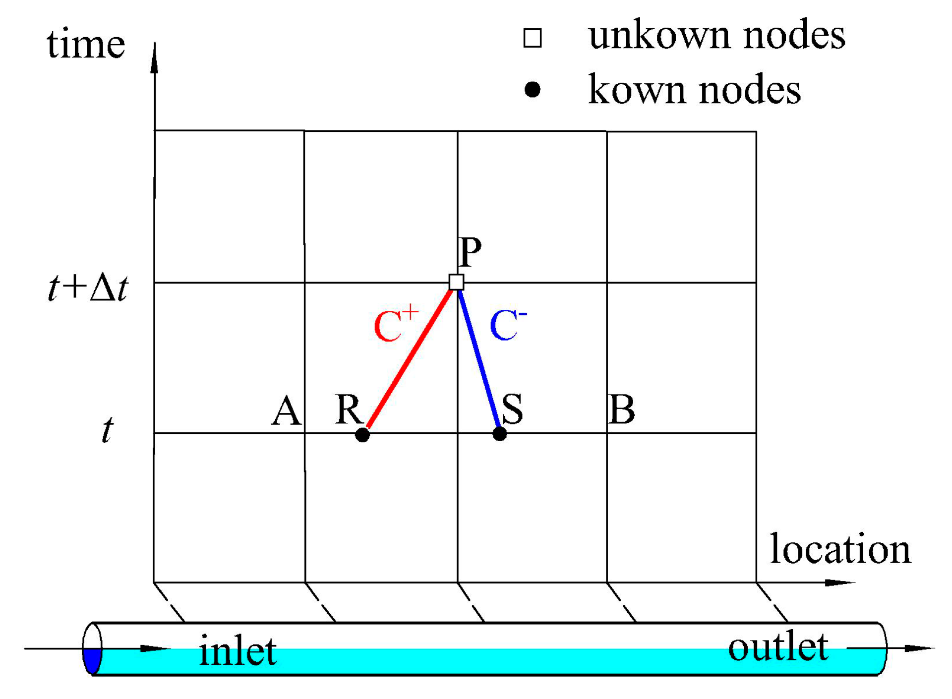
The first task to be carried out immediately after the construction or repair of a water supply system is to completely fill the pipeline with water. The process of filling can be regarded as an open channel flow condition, as the water surface is in direct contact with the atmosphere. At this stage, the pressure wave speed is usually much lower than the pressured pipe flow. According to momentum and continuity equations, the MOC [23] is set up based on Equations (1)–(4). Figure 1 shows the node meshing of the open channel flow.
Equations (1)–(4) are
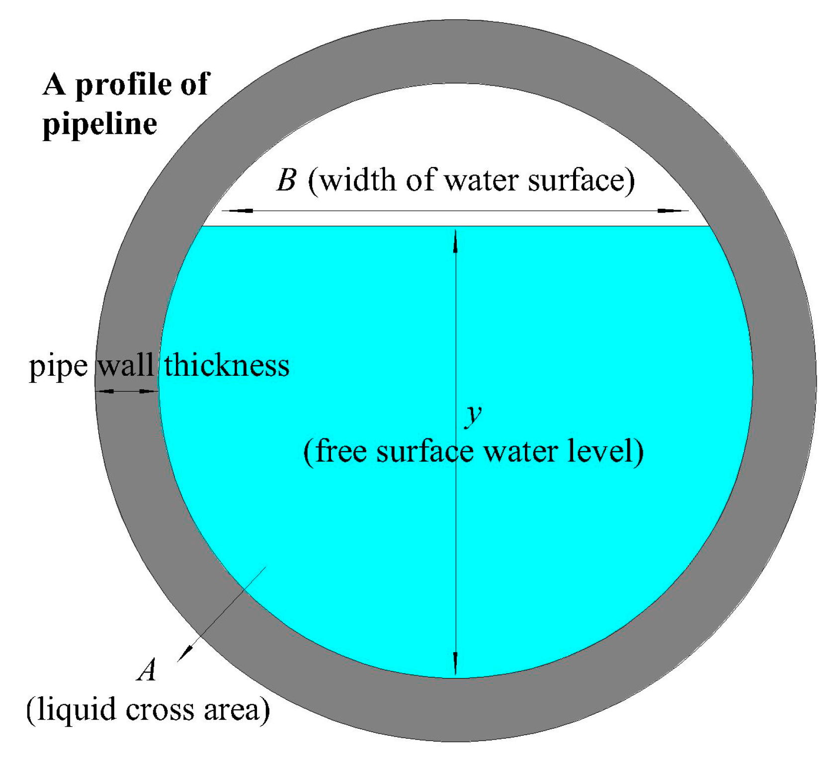
where and are the fluid velocities at the nodes and , respectively; and are the water levels at the nodes and , respectively; and are the energy gradients at the nodes and , respectively; and are the cross-sectional areas of the liquid at the nodes and , respectively; and are the locations at the nodes and , respectively; is the acceleration due to gravity; denotes the time step; is the inlet discharge in the transverse direction per unit length; is the original energy gradient due to the inclination between the pipeline and the horizontal plane; and is defined to be equal to , where denotes the width of the water surface at that node, as shown in Figure 2.
2.1.2. Stage 2: Pressured Pipe Flow
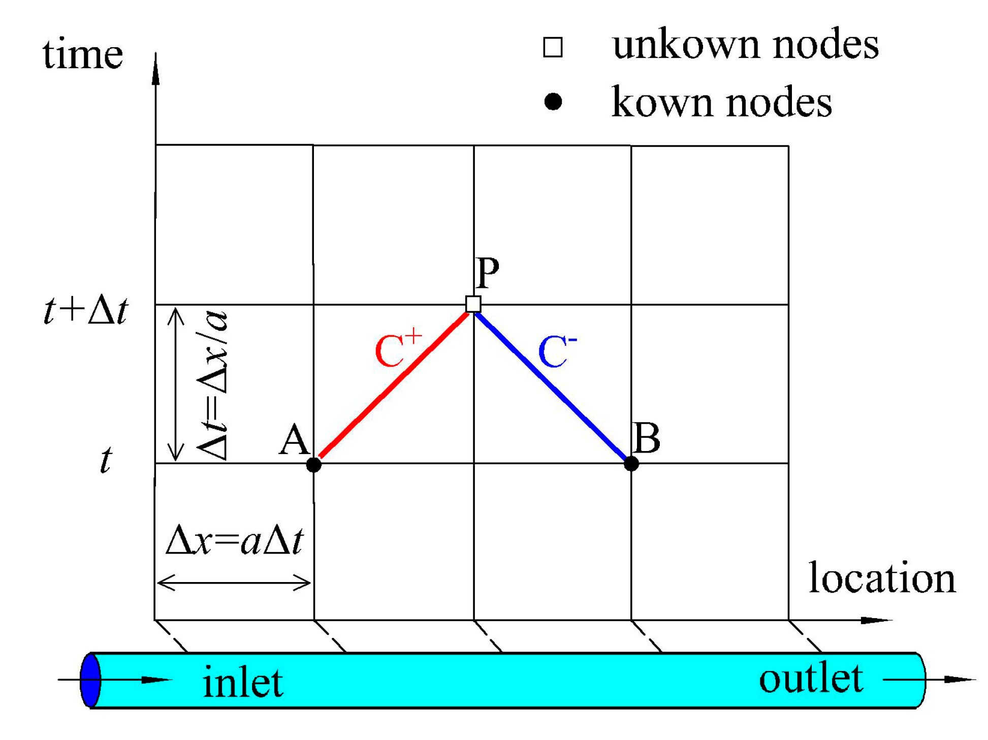
After the pipe is filled, the liquid flow becomes pressured, and the pressure wave speed multiplies immediately. The characteristic equations are expressed as Equations (5) and (6) [23], and the node meshing is shown in Figure 3:
where , , and are the water levels at the nodes P, A, and B, respectively, when they are higher than the diameter of the pipe; is the pressure wave speed; and , , and are the discharges through the profiles at the respective nodes P, A, and B.
2.1.3. Combination Method
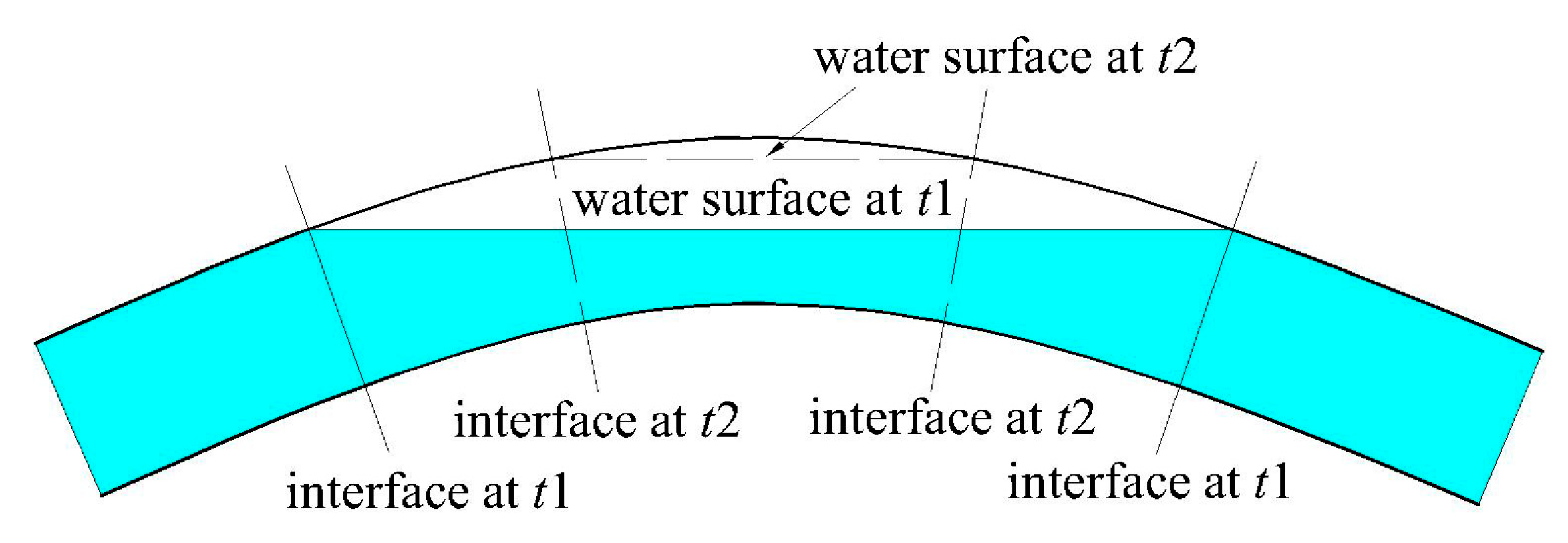
In the water filling process of a water supply pipeline system, the two conditions mentioned above, namely the free surface pipe flow and pressured pipe flow, usually exit at the same time due to the layout of the pipeline. When the lower zone is already filled, the higher zone may still be at the free surface flow stage. The interfaces of the two parts, namely the filled and unfilled parts, move as the water keeps filling, as shown in Figure 4.
It would be too complex to track each interface and separate the nodes into different parts and carry out the calculations by using different numerical methods. Moreover, the boundary conditions at the interfaces are another problem for the simulation. Thus, to simulate the entire water filling process, the two equation sets were combined.
Using the slot method [29], assuming to be equal to and the pressure wave speed in pressured flow , the two models are combined into a corresponding model. Therefore, the width of the assumptive slot is given by . For a circular tube, the assumptive slot is shown in Figure 5.
In the case of a tube of diameter 1.0 m, the pressure wave speed of the pressured pipe flow is assumed to be 1000 m/s. The parameters of a pipeline profile with the virtual slot are shown in Figure 6. Thus, the two conditions are combined into one corresponding equation set, and therefore can be simulated in a single model using Equations (1)–(4) as a general presentation. The solution can be accessed in FORTRAN, expressing the derived equations as follows:
It should be listed here that in this model, an instability may occur with an improper simulation of , the energy gradient. Usually, when the water is partly filled, it can be calculated approximately as , where is the wetted perimeter. However, when the water level is tiny, this approximate solution loses reliability. In this research, when the water level is less than 0.1 m, the energy gradient is assumed to be equal to , the original energy gradient, to avoid the instability of program running.
2.2. Boundary Conditions
In this study, a single pipeline with a surge tank is considered as an example. The water level H0 in an upstream reservoir is regarded as a constant at 10 m. A gate is set at the upstream entrance of the pipeline to control the inlet discharge, and a valve is set at the downstream exit to control the outlet. A surge tank is located in the middle of the pipeline to control the extreme pressure in water hammers. The parameters are listed in Table 1. The model of the water supply system is shown in Figure 7.
2.2.1. Surge Tank Boundary Model
A surge tank is an effective pressure control device in a water supply pipeline system that can reduce the density of both positive and negative extreme pressures in the event of the occurrence of a water hammer. Normally, a surge tank consists of a joint connector and a tank body. The tank body is used to store enough of a volume of water to maintain the pressure at a stable range when the water hammer occurs. The joint connector is used to connect the tank body and the pipeline. A suitable design of the connector can help to improve the pressure control ability of the surge tank [25].
In the combination model, the boundary condition of the surge tank is divided due to two different water level situations. The first situation is that the water level at the position of the joint has not reached the top inside the pipe. At this period, the surge tank can be ignored, and the numerical solution is similar to that of the other normal inner nodes in the pipeline. The other situation is that the water level at the position of the joint is greater than the diameter of the pipeline, which indicates that the water has already filled the pipe at that point. In this case, the characteristic of surge tanks must be considered for the boundary condition. The controlling equation set consists of two characteristic lines, and the feature of the surge tank is as shown below:
where and are the liquid velocities at the i and j profiles, respectively; and are the liquid-filled cross-sectional areas at the i and j profiles, respectively; and are the liquid velocities at the i and j profiles at the last time step, respectively; and are the liquid-filled cross-sectional areas at the i and j profiles at the last time step, respectively; is the water level in the surge tank at the last time step; and is the cross-sectional area of the surge tank body. Figure 8 shows the detailed parameters and the logical figure of a surge tank. After analytical derivation, the boundary condition of a surge tank can be expressed as follows:
2.2.2. Upstream and Downstream Boundary Models
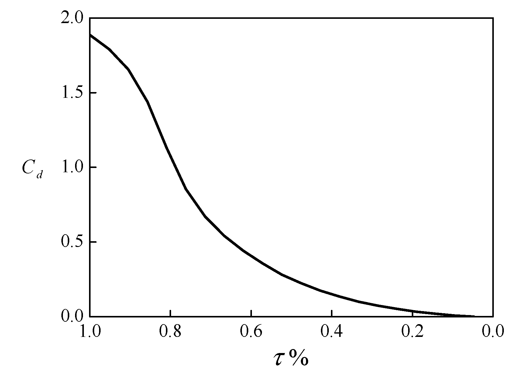
Two controlling equations must be considered for the upstream boundary condition. The first is the discharge equation of the gate, which is a flow control device. The discharge characteristic of the gate is shown in Figure 9, and the discharge equation of the gate is as follows:
is the discharge coefficient of the gate, which depends on the valve performance curve and opening ratio at a particular time; is the cross-sectional area of the gate; y1 is the water level at the first profile in the pipeline; and denotes the pressure difference between both of its sides. The discharge can be obtained by multiplying the fluid velocity and the cross-sectional area.
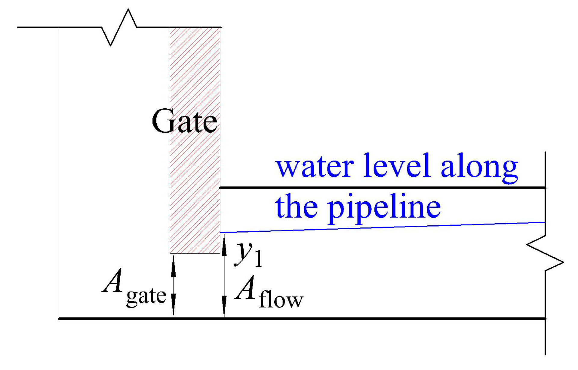
In addition, there is an inverse characteristic equation set to control the boundary condition. The combined equation set is as follows:
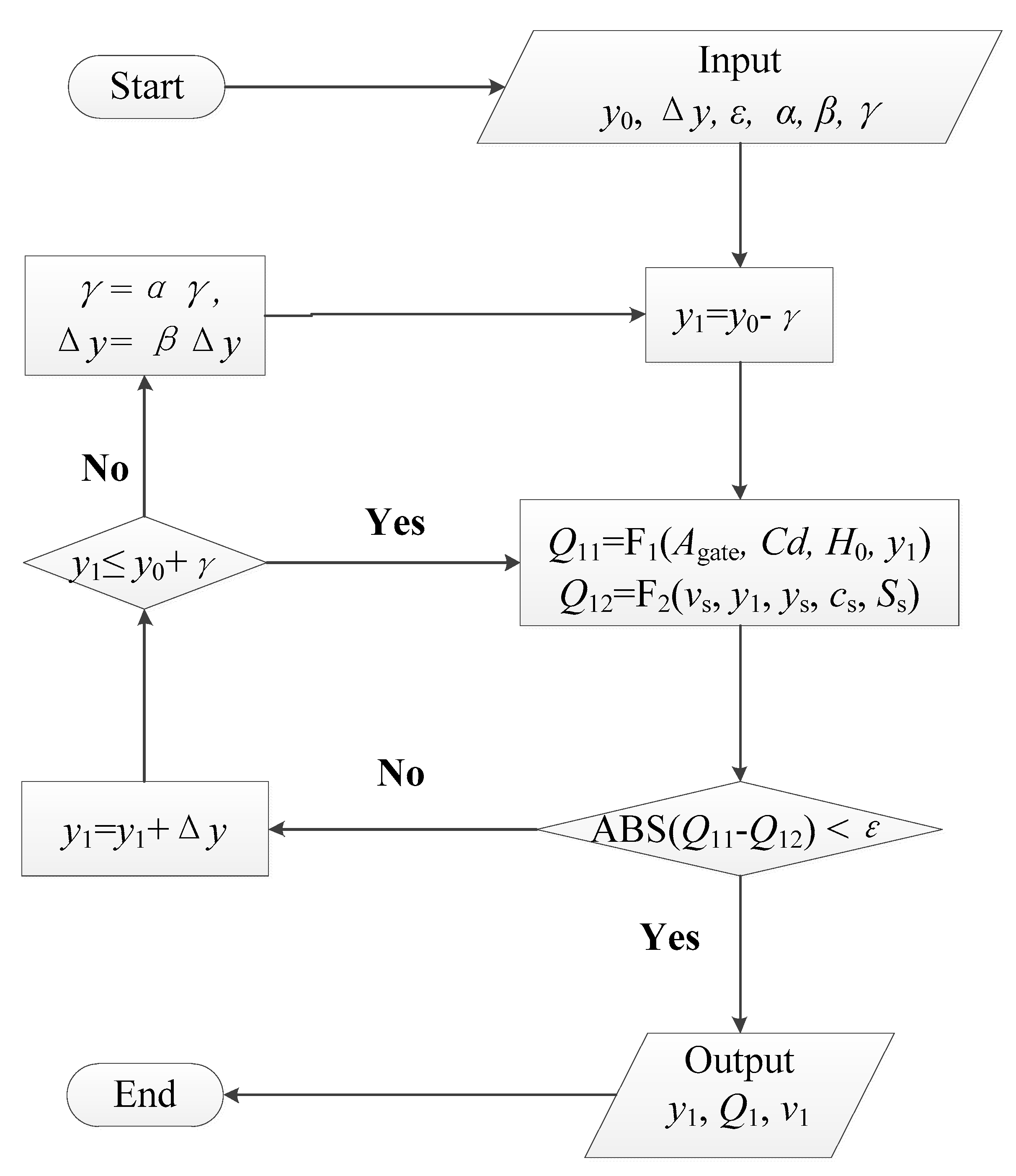
where is the flow velocity at the first profile in the pipeline, and is the liquid cross-sectional area at that profile. Figure 10 shows the details of the upstream boundary parameters. This complex equation set is solved by DFM, the logical loop chart of which is shown as Figure 11. By limiting the allowable error less than 0.1, the program can be equipped with reliable stability.
At the downstream boundary, the valve is the flow control device, whose rapid closing causes a water hammer. In the water filling process, it is usually entirely closed to prevent any outflow. Using Equation (1), the downstream boundary condition is as follows:
2.3. Proposed Double Forward Method
As it is too complex to obtain an analytical solution of the combined equation set, a numerical iteration solution known as the double forward method (DFM) is proposed in this study to determine the upstream boundary condition. Figure 11 shows the logical flow chart of the DFM.
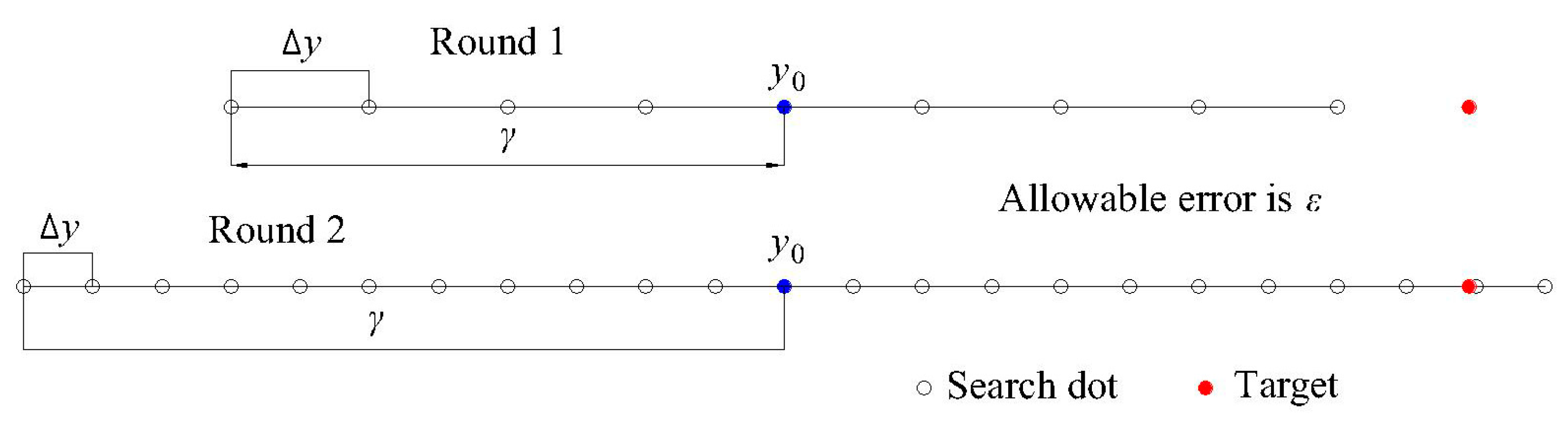
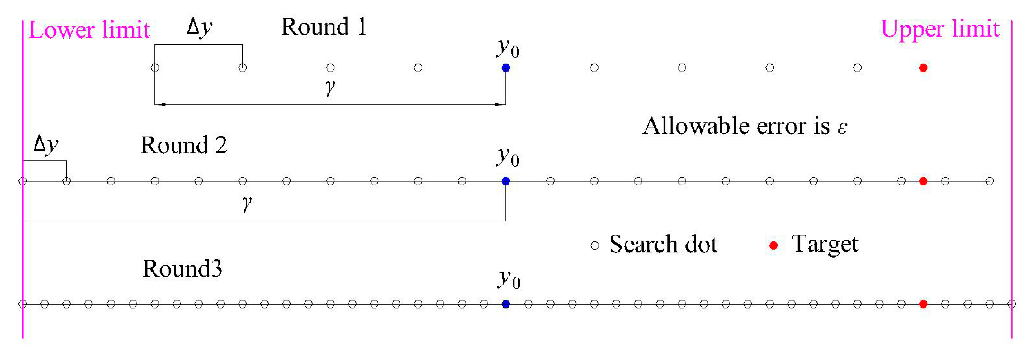
Here, y0 is the water level of the first profile at the last time step and the input as the initial value in the iteration process to obtain y1, the water level of the first profile at the new time step; ∆y is the search step; ε is the allowable error, which represents the accuracy; γ is the search zone; and α ∈ (1, +∞) and β ∈ (0, 1) are the forward coefficients of γ and ∆y, respectively. Figure 12 shows a two-round iteration search process of the DFM.
The objective of using the DFM is to improve the search accuracy and expand the search zone when it is necessary to find the target. When the demand for accuracy is not rigid, the solution can be obtained by using a relatively large search step in a fairly small zone: The greater the demand for a high accuracy in the solution, the more rounds that run. The DFM is always effective in finding a solution to satisfy the demands, though the time taken may be comparatively longer when the demand for accuracy is rigid. Apart from the requirement of accuracy, the choice of a suitable initial point is significant to control the time for the calculation. In this example, the water level of the first profile at the last time step was chosen as the initial point, which was close to the target in most situations.
3. Application in a Typical Filling Process
On the basis of the established model for the simulation, the water filling process in a pipeline system can be divided into two stages. In the first stage, the front surface of the water runs from the upstream gate to the downstream valve. During this period, the entire system is considered to be a free surface flow. As only a part of the pipeline is filled, the pressure does not reach a high level and can be quickly released by a change in the volume. After some time, Stage 2 is reached, in which the pipeline is completely filled with water. Subsequently, the pipeline is affected by a water hammer condition, as there is no room for the release of pressure of the water by enlarging its volume in the pipeline. Therefore, by using the DFM based on the MOC to obtain the upstream boundary condition, the water filling process is appropriately simulated.
3.1. Free Surface Flow Stage
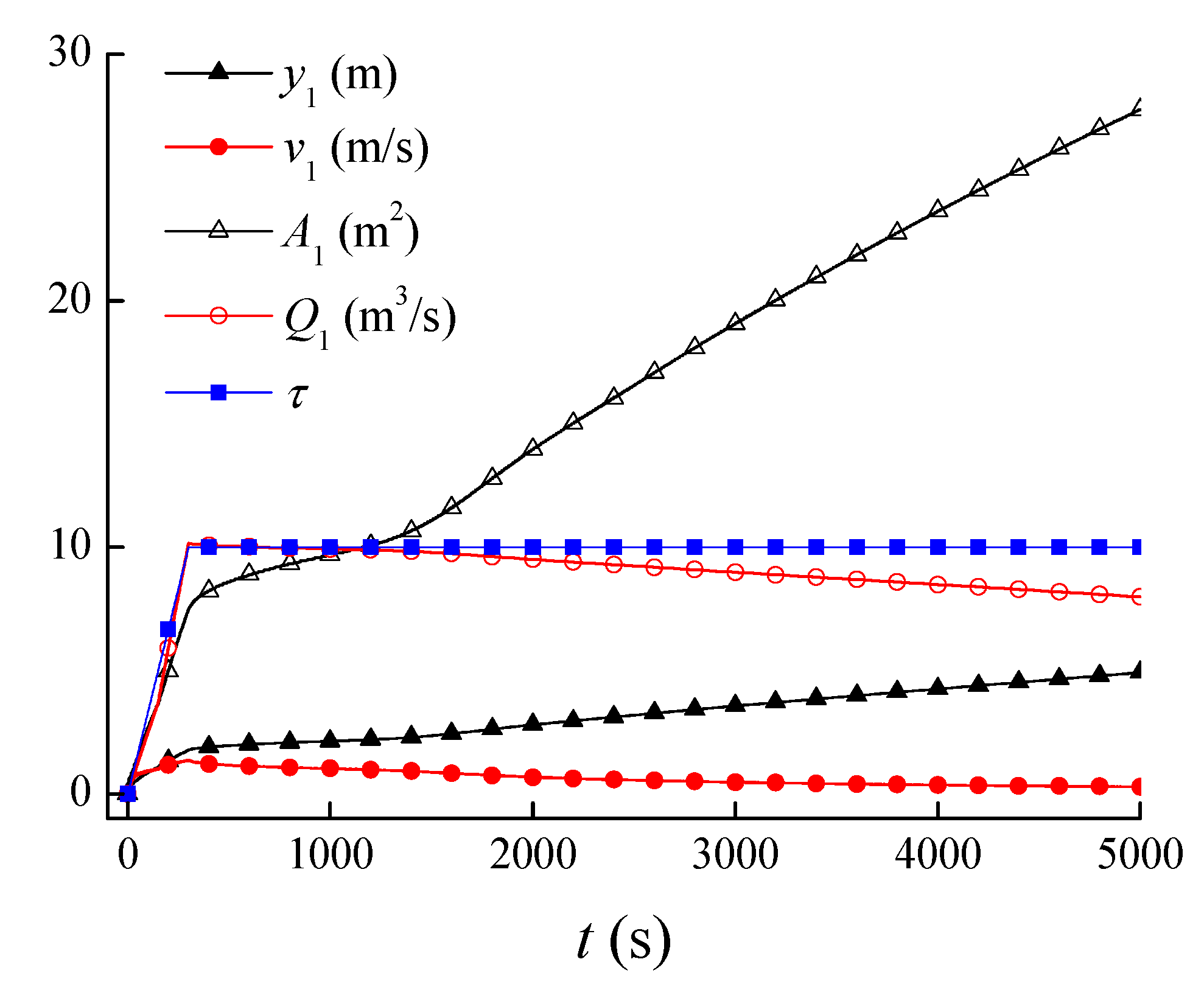
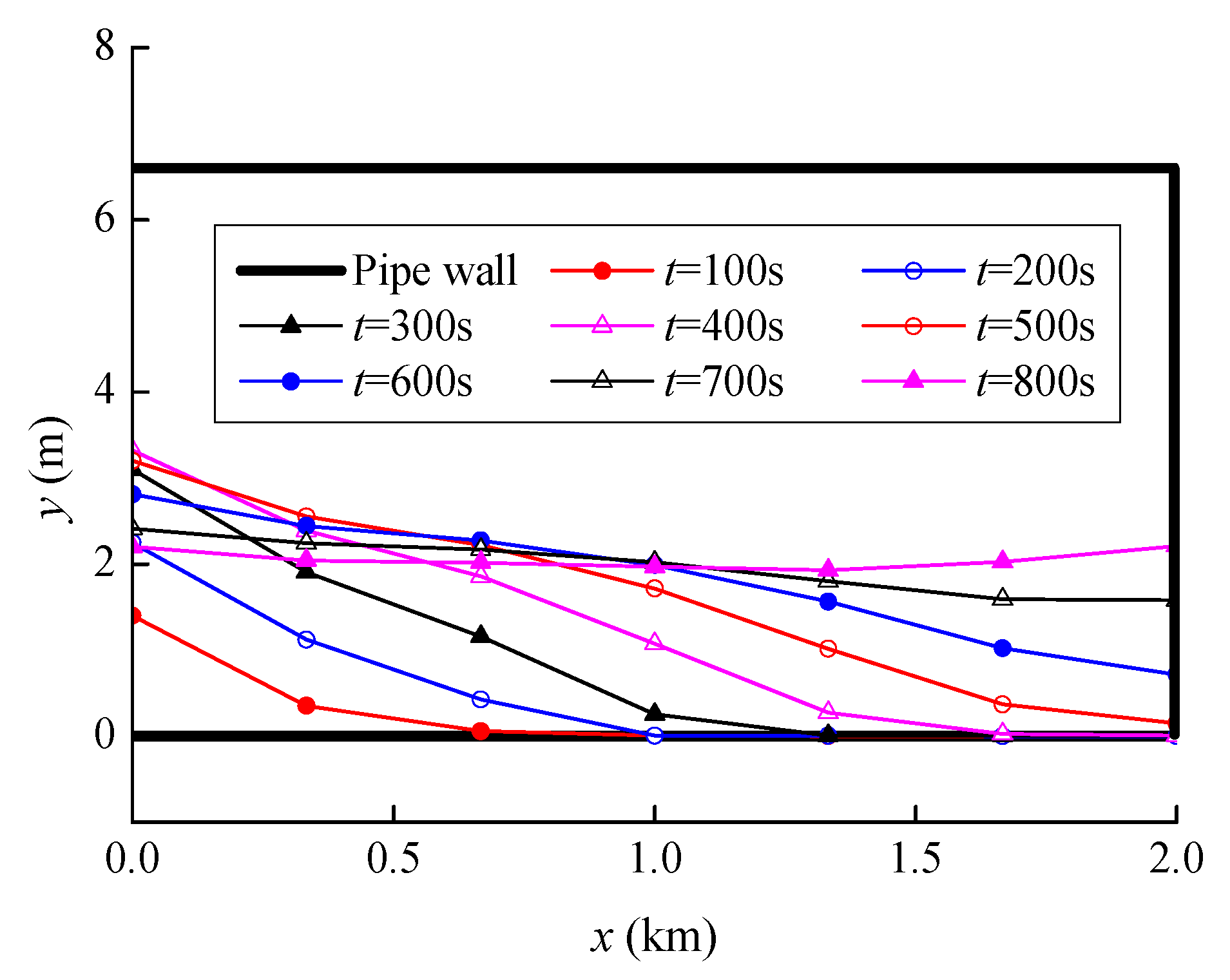
In the water filling process, the open ratio of the upstream gate increases from 0.0 to 0.1 in 10 min, while the downstream valve is kept tightly closed. At the beginning of the water filling process, the flow velocity rapidly rises to a relatively high value and then reduces slowly as the water level increases smoothly (as the discharge of the first profile). Meanwhile, the liquid cross-sectional area and water level continue to rise. Figure 13 shows the changing process of the parameters of the first profile during the filling process (Stage 1), and Figure 14 shows the water level along the pipeline during the first 800 s.
In this period, there is a theoretical limit to the DFM searching area. The water level cannot be lower than the bottom of the pipe, as there is no negative pressure. The upper limit can be set as the diameter of the pipe, as it is not completely filled. Thus, the calculating time is shortened. Figure 15 shows the theoretical limits of the searching zones in Stage 1.
3.2. Pressured Flow Stage
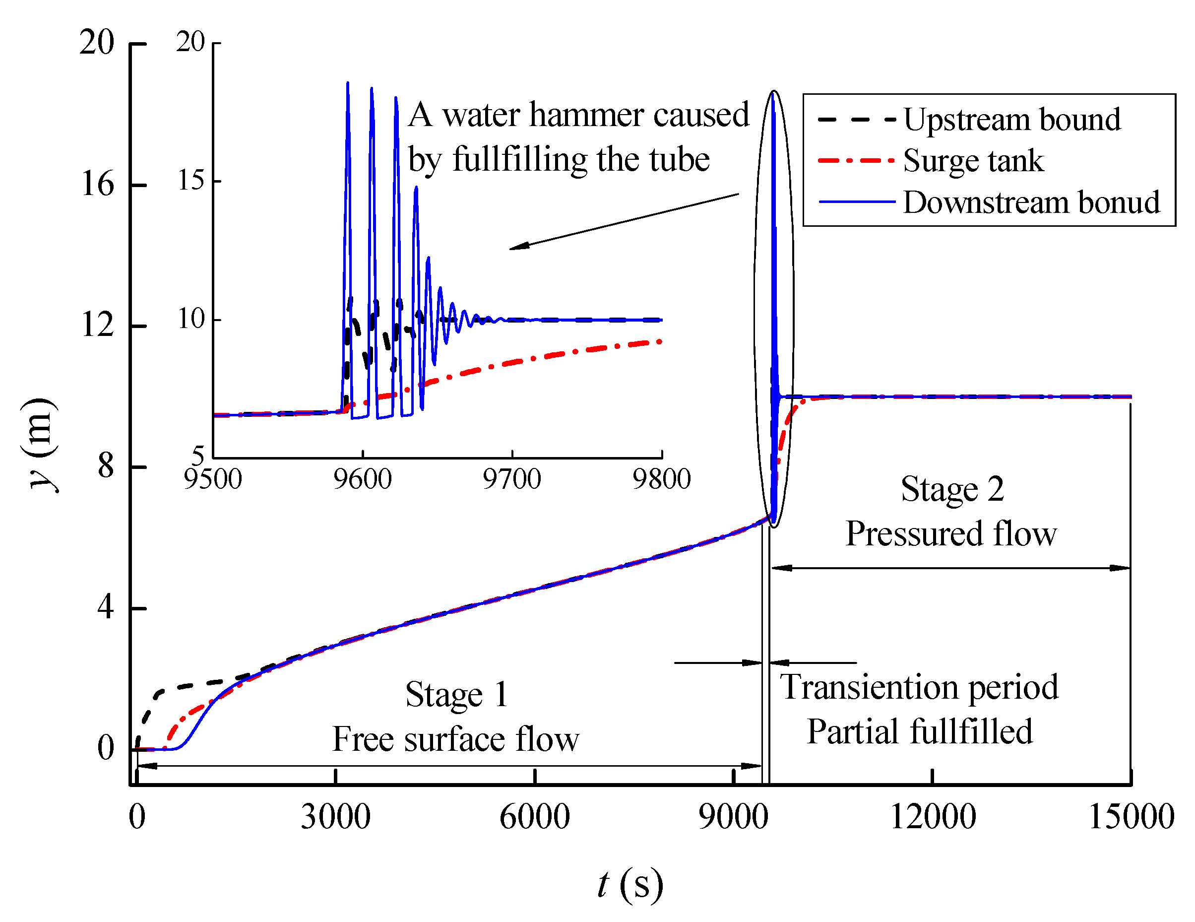
After some time, only a part of the pipeline is filled, and the pressure does not reach a high level in this period, as it can be quickly released by a change in the volume. However, the pipeline suffers an extreme pressure wave once it is completely filled, and Stage 1 switches over to Stage 2. The pressure cannot be released immediately, as there is no room left for the volume of water to expand and release the extreme pressure. The surge tank set in the middle of the pipeline becomes useful at this stage, as it effectively reduces the intensity of the extreme pressure. Figure 16 shows the water level (which represents the hydraulic head after the pipe is filled) at the upstream bound profile, the surge tank, and the downstream bound profile. At the beginning of Stage 1, the water level at the upstream bound grows in advance. Shortly, after the water front reaches the downstream bound, the water level along the pipeline grows in a relatively corresponding speed until the pipeline is filled. When the transient occurs as the pipeline is filled, the intensity of the pressure wave at the downstream bound turns out to be severe, while the fluctuation at the upstream bound is much less. This is because, in this period, the surge tank reduces much of the water hammer energy delivered from the downstream, and the upstream reservoir also provides a stable water head at the upstream side.
3.3. Validation
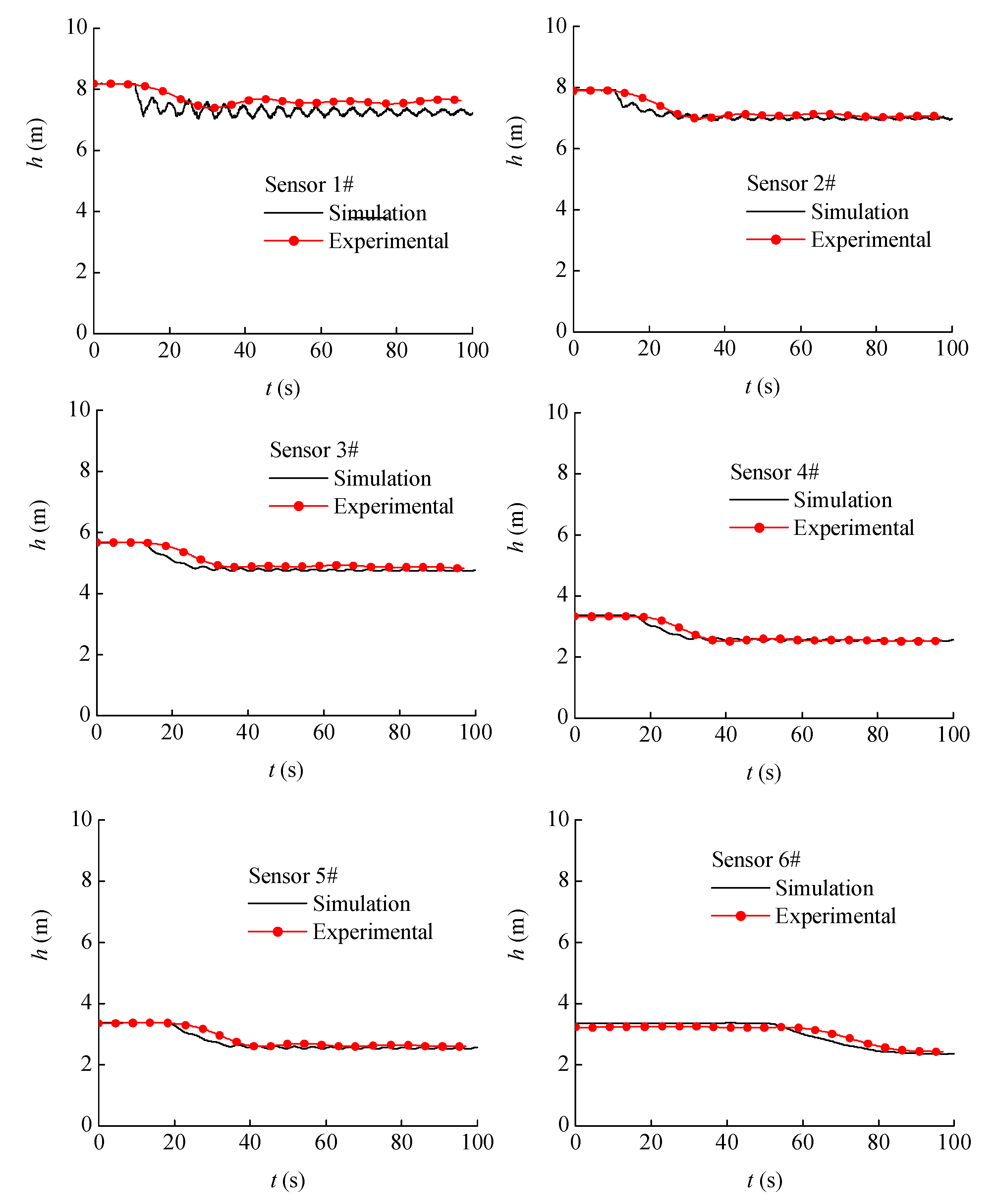
For validation of the DFM, a transient process caused by partly closing the upstream valve, where part of the pipeline is pressured flow and the other is free surface flow, was numerically simulated using the DFM and was experimentally measured for comparison. Six sensors were located from upstream to downstream for recording the pressure changing process. The comparison between experimental data and the simulation is shown in Figure 17. As can be seen, the simulation results basically agreed with the experimental data on the trend of the pressure processes at all six sensors. In detail, the oscillation shown in the simulation results was more obvious than the measured data. This may have been a reflection of air contained in the pressured part or a little leakage in the experiment pipeline, since both of these can help reduce water hammer intensity and oscillation.
It should be listed here that the influence of DFM on the accuracy of simulations only depends on the allowable error set in the searching loops. The accuracy of the simulation models mainly depends on the controlling equations of the boundary conditions, especially their assumptions. However, with the use of DFM, complex boundary conditions can be solved with fewer assumptions and in this way improve the reliability of simulation models.
4. Discussion
Boundary conditions are always the focal points in establishing a high-accuracy numerical model in transient flow simulations, but most of them are hard to define perfectly due to the complex physical parameters of devices. It was found that many complex devices could be reduced to compact, manageable, mathematically tractable forms that preserved the physical nature of the devices being modeled, which proved to be useful, as many of the boundary conditions in previous research have been determined on this basis [22]. For a water supply pipeline system, where there is an upstream reservoir and the upstream gate remains at a stable open ratio, the upstream boundary condition is relatively simple. In this situation, the upstream hydraulic head is regarded as a constant, as the fluctuation of the water level in the reservoir can be ignored during a transient water hammer process [17,19]. However, in the case of an operation on the upstream gate, there may be changes in the discharge coefficient that depend on the upstream water level, the downstream water level, and the intensity of rainfall. The gate opens to a higher level when this is required to enhance the water supply discharge, whereas it is closed when the water volume is to be restored for the generation of electricity. Thus, the upstream boundary condition must combine three equations: (i) The constant upstream reservoir water level, (ii) a reverse characteristic line equation, and (iii) the gate open ratio and its corresponding discharge coefficient. An analytical solution and a closing law for reducing the intensity of the water hammer has been researched [30]. Furthermore, it is more complex if a pump station, to provide energy to pressurize the water to flow from upstream to downstream, is located in front of the upstream gate. This has been dealt with analytically by considering the pump as another boundary condition and solving the equations separately [26,31]. However, the water filling process is even more complicated, as the water level in the pipeline continuously changes, and the water-filled cross-sectional area differs at each time step. Therefore, the combined equation set given in Equation (14) cannot be easily solved analytically, especially when the mapping relationship between the water level and liquid cross-sectional area is complex. For example, in a pipe profile of an irregular shape, the mapping function is described as a set of piecewise functions rather than as a single equation. Hence, the upstream boundary condition is solved numerically by an iterative solution. An appropriate set of permissible error and initial parameters is significant for controlling the time of calculation. The proposed method is not only suitable in the case of the upstream boundary condition, but also in all kinds of combination equation sets of complex boundary conditions. As the permissible error is freely defined, the accuracy of the DFM is controllable and the boundary conditions are not too simplified, and therefore the simulations are more reliable. Through various simulations in previous research [32], it has been found that when the time step ∆t is valued at no greater than 0.01 s, where the location step is correspondingly about 10 m/s, the program can avoid instability caused by improper meshing. Of course, for free surface flow, as the pressure wave speed is much less, it is too sparse to accurately track the water front of the water filling progress. However, as a feature of a circular tube, when the pipeline is nearly filled, the pressure wave speed differs little from pressure flow, and the abrupt pressure change of the water hammer caused by the filling action is still reliable.
5. Conclusions
The complex boundary conditions of numerical models are usually simplified to derive an analytical solution. In this study, a double forward method (DFM) was proposed to simulate complex boundary conditions in an algorithmic way, and a water filling model of a water supply pipeline system was developed to simulate the water filling process by using the slot method. The surge tank boundary condition was improved to fit both stages of the pipe filling process. In addition, experimental data of a transient process were measured to validate the simulation model, which turned out to show good agreement with the numerical simulations. The accuracy of the DFM can be controlled by limiting the permissible error, while the reliability of the whole program still depends on proper meshing and boundary solutions. Moreover, the limits of the searching zone are defined according to the physical parameters to shorten the time of calculation.
Author Contributions
Methodology, B.Z. and W.W.; software, B.Z.; validation, B.Z. and W.W.; formal analysis, W.W. and L.F.; investigation, B.Z. and L.F.; resources, W.W.; data curation, B.Z. and L.F.; writing—original draft preparation, B.Z.; writing—review and editing, B.Z. and W.W.; supervision, W.W.; project administration, W.W.; funding acquisition, W.W.
Funding
This research work was supported by the National Natural Science Foundation of China (Grant Nos. 51779216, 51279175) and the Zhejiang Provincial Natural Science Foundation of China (Grant No. LZ16E090001).
Acknowledgments
This research is supported by China Scholarship Council, Zhejiang University and University of Cambridge.
Conflicts of Interest
The authors declare no conflict of interest.
Abbreviations
| t | time (s) |
| ∆t | time step (s) |
| v | flow velocity (m/s) |
| g | acceleration of gravity (m/s2) |
| c | wave speed in free surface flow (m/s) |
| y | water level (m) |
| S | energy gradient |
| q | inlet discharge from the transverse direction within a unit length (m3/s) |
| A | flow-filled cross area (m2) |
| B | water surface width (m) |
| H | pressure head (m) |
| Q | discharge (m3/s) |
| x | distance along pipe from inlet (m) |
| ∆x | length of segment (m) |
| a | speed of pressure wave in pressured flow (m/s) |
| f | Darcy friction factor |
| D | main pipe diameter (m) |
| Cd | discharge coefficient |
| τ | valve opening ratio |
| ∆y | water level step (m) |
| ε | allowable error (m3/s) |
| α | forward coefficient |
| β | forward coefficient |
| γ | searching range (m) |
| DFM | double forward method |
| MOC | method of characteristics |
References
- Boulos, P.F.; Karney, B.W.; Wood, D.J.; Lingireddy, S. Hydraulic transient guidelines for protecting water distribution systems. J. Am. Water Work Assoc. 2005, 97, 111–124. [Google Scholar] [CrossRef]
- Arnold, J.G.; Srinivasan, R.; Muttiah, R.S.; Williams, J.R. Large area hydrologic modeling and assessment—Part 1: Model development. J. Am. Water Resour. Assoc. 1998, 34, 73–89. [Google Scholar] [CrossRef]
- Fang, H.Q.; Chen, L.; Dlakavu, N.; Shen, Z.Y. Basic Modeling and simulation tool for analysis of hydraulic transients in hydroelectric power plants. IEEE Trans. Energy Convers. 2008, 23, 834–841. [Google Scholar] [CrossRef]
- Bergant, A.; Simpson, A.R.; Vitkovsky, J. Developments in unsteady pipe flow friction modelling. J. Hydraul. Res. 2001, 39, 249–257. [Google Scholar] [CrossRef]
- Bergant, A.; Simpson, A.R.; Tijsseling, A.S. Water hammer with column separation: A historical review. J. Fluids Struct. 2006, 22, 135–171. [Google Scholar] [CrossRef]
- Martins, N.M.C.; Delgado, J.N.; Ramos, H.M.; Covas, D.I.C. Maximum transient pressures in a rapidly filling pipeline with entrapped air using a CFD model. J. Hydraul. Res. 2017, 55, 506–519. [Google Scholar] [CrossRef]
- Lingireddy, S.; Wood, D.J.; Zloczower, N. Pressure surges in pipeline systems resulting from air releases. J. Am. Water Works Assn. 2004, 7, 88–94. [Google Scholar] [CrossRef]
- Martin, C.S. Proceedings of the 2nd International Conference on Pressure Surges; The Bedford Press: London, UK, 1976; pp. F2/15–F2/28. [Google Scholar]
- Triki, A. Water-hammer control in pressurized-pipe flow using a branched polymeric penstock. J. Pipeline Syst. Eng. Pract. 2017, 8, 04017024. [Google Scholar] [CrossRef]
- Tian, W.X.; Su, G.H.; Wang, G.P.; Qiu, S.Z.; Xia, Z.J. Numerical simulation and optimization on valve-induced water hammer characteristics for parallel pump feedwater system. Ann. Nucl. Eng. 2008, 35, 2280–2287. [Google Scholar] [CrossRef]
- Kim, H.; Kim, S.; Kim, Y.; Kim, J. Optimization of operation parameters for direct spring loaded pressure relief valve in a pipeline system. J. Pressure Vessel Technol. 2018, 140, 051603. [Google Scholar] [CrossRef]
- Kim, H.; Baek, D.; Kim, S. Exploring integrated impact of temperature and flow velocity on chlorine decay for a pilot-scale water distribution system. Desalin. Water Treat. 2019, 138, 265–269. [Google Scholar] [CrossRef]
- Apollonio, C.; Balacco, G.; Fontana, N.; Giugni, M.; Marini, G.; Piccinni, A.F. Hydraulic transients caused by air expulsion during rapid filling of undulating pipelines. Water 2016, 8, 25. [Google Scholar] [CrossRef]
- Balacco, G.; Apollonio, C.; Piccinni, A.F. Experimental analysis of air valve behaviour during hydraulic transients. J. Appl. Water Eng. Res. 2015, 3, 3–11. [Google Scholar] [CrossRef]
- Chaudhry, M.; Hussaini, M. Second-order accurate explicit finite-difference schemes for waterhammer analysis. J. Fluids Eng. 1985, 107, 523–529. [Google Scholar] [CrossRef]
- Kochupillai, J.; Ganesan, N.; Padmanabhan, C. A new finite element formulation based on the velocity of flow for water hammer problems. Int. J. Press. Vessels Pip. 2005, 82, 1–14. [Google Scholar] [CrossRef]
- Izquierdo, J.; Iglesias, P.L. Mathematical modelling of hydraulic transients in simple systems. Math. Comput. Modell. 2002, 35, 801–812. [Google Scholar] [CrossRef]
- Karadzic, U.; Bulatovic, V.; Bergant, A. Valve-Induced water hammer and column separation in a pipeline apparatus. Strojniski Vestn. J. Mech. Eng. 2014, 60, 742–754. [Google Scholar] [CrossRef]
- Zhang, B.; Wan, W.; Shi, M. Experimental and numerical simulation of water hammer in gravitational pipe flow with continuous air entrainment. Water 2018, 10, 928. [Google Scholar] [CrossRef]
- Coronado-Hernandez, O.E.; Fuertes-Miquel, V.S.; Besharat, M.; Ramos, H.M. Experimental and numerical analysis of a water emptying pipeline using different air valves. Water 2017, 9, 98. [Google Scholar] [CrossRef]
- Wan, W.; Li, F. Sensitivity analysis of operational time differences for a pump–valve system on a water hammer response. J. Pressure Vessel Technol. 2016, 138, 011303. [Google Scholar] [CrossRef]
- Karney, B.W.; McInnis, D. Efficient calculation of transient flow in simple pipe networks. J. Hydraul. Eng. 1992, 118, 1014–1030. [Google Scholar] [CrossRef]
- Wylie, E.B.; Streeter, V.L. Fluid Transients; McGraw-Hill International Book Co.: New York, NY, USA, 1978. [Google Scholar]
- Wan, W.; Huang, W. Investigation on complete characteristics and hydraulic transient of centrifugal pump. J. Mech. Sci. Technol. 2011, 25, 2583–2590. [Google Scholar] [CrossRef]
- Wan, W.; Zhang, B. Investigation of water hammer protection in water supply pipeline systems using an intelligent self-controlled surge tank. Energies 2018, 11, 1450. [Google Scholar] [CrossRef]
- Wan, W.; Huang, W. Investigation of fluid transients in centrifugal pump integrated system with multi-channel pressure vessel. J. Pressure Vessel Technol. 2013, 135, 9. [Google Scholar] [CrossRef]
- Hou, Q.; Zhang, L.X.; Tijsseling, A.S.; Kruisbrink, A.C.H. Rapid filling of pipelines with the SPH particle method. In International Conference on Advances in Computational Modeling and Simulation; Lixiang, Z., Ed.; Elsevier Science Bv: Amsterdam, The Netherlands, 2012; pp. 38–43. [Google Scholar]
- Balacco, G.; Fontana, N.; Apollonio, C.; Giugni, M.; Marini, G.; Piccinni, A.F. Pressure surges during filling of partially empty undulating pipelines. ISH J. Hydraul. Eng. 2018, 1–9. [Google Scholar] [CrossRef]
- Chaudhry, M.H. Applied Hydraulic Transients; Van Nostrand Reinhold: New York, NY, USA, 1979. [Google Scholar]
- Vakil, A.; Firoozabadi, B. Investigation of Valve-Closing Law on the Maximum Head Rise of a Hydropower Plant. Sci. Iranica Trans. B-Mech. Eng. 2009, 16, 222–228. [Google Scholar]
- Pepa, D.; Ursoniu, C.; Gillich, G.R.; Campian, C.V. Water hammer effect in the spiral case and penstock of Francis turbines. In International Conference on Applied Sciences; Lemle, L.D., Jiang, Y., Eds.; Iop Publishing Ltd.: Bristol, UK, 2017. [Google Scholar]
- Wan, W.; Huang, W. Water hammer simulation of a series pipe system using the MacCormack time marching scheme. Acta Mech. 2018, 229, 3143–3160. [Google Scholar] [CrossRef]
Figure 1.
Meshes of open channel flow. where A, B and P are the gird nodes in the meshing of pressured flow, R and S are the modified adjacent nodes in free surface flow. C+ and C- are the characteristic lines.
Figure 1.
Meshes of open channel flow. where A, B and P are the gird nodes in the meshing of pressured flow, R and S are the modified adjacent nodes in free surface flow. C+ and C- are the characteristic lines.

Figure 2.
Parameters in the profile of a pipeline.

Figure 3.
Meshes of pressured flow.

Figure 4.
Interfaces of the two parts.

Figure 5.
Assumptive slot of circular tube.

Figure 6.
Parameters of a profile with a virtual slot.

Figure 7.
Model of a single pipeline with a surge tank.

Figure 8.
Logical boundary condition of a surge tank.

Figure 9.
Discharge coefficient of the gate.

Figure 10.
Details of upstream boundary parameters.

Figure 11.
Logical flow chart of the double forward method (DFM).

Figure 12.
Logical meshing of the DFM.

Figure 13.
Parameters of the first profile in a water filling process (Stage 1).

Figure 14.
Water level along the pipeline in a water filling process (Stage 1).

Figure 15.
Theoretical limits of searching zones.

Figure 16.
Water level at specific points in the entire water filling process.

Figure 17.
Comparison between the simulation and the experiment on a transient process.


Table 1.
Parameters of the pipeline system.
| Reservoir | Dam | Gate | Pipeline | Surge Tank | Valve | ||
|---|---|---|---|---|---|---|---|
| Water level | Height | Nominal area | Cross area | Length | Cross area | Water level | Height |
| 10 m | 15 m | 25 m2 | 35 m2 | 2000 m | 100 m2 | 10 m | 15 m |
© 2019 by the authors. Licensee MDPI, Basel, Switzerland. This article is an open access article distributed under the terms and conditions of the Creative Commons Attribution (CC BY) license (http://creativecommons.org/licenses/by/4.0/).
Share and Cite
MDPI and ACS Style
Zhang, B.; Wan, W.; Fan, L. Investigation into Complex Boundary Solutions of Water Filling Process in Pipeline Systems. Water 2019, 11, 641. https://doi.org/10.3390/w11040641
AMA Style
Zhang B, Wan W, Fan L. Investigation into Complex Boundary Solutions of Water Filling Process in Pipeline Systems. Water. 2019; 11(4):641. https://doi.org/10.3390/w11040641
Chicago/Turabian StyleZhang, Boran, Wuyi Wan, and Leilei Fan. 2019. "Investigation into Complex Boundary Solutions of Water Filling Process in Pipeline Systems" Water 11, no. 4: 641. https://doi.org/10.3390/w11040641
Note that from the first issue of 2016, this journal uses article numbers instead of page numbers. See further details here.