Assessing the Vulnerability of Aquatic Macroinvertebrates to Climate Warming in a Mountainous Watershed: Supplementing Presence-Only Data with Species Traits

 , ,
, ,
Abstract
:1. Introduction
2. Methods
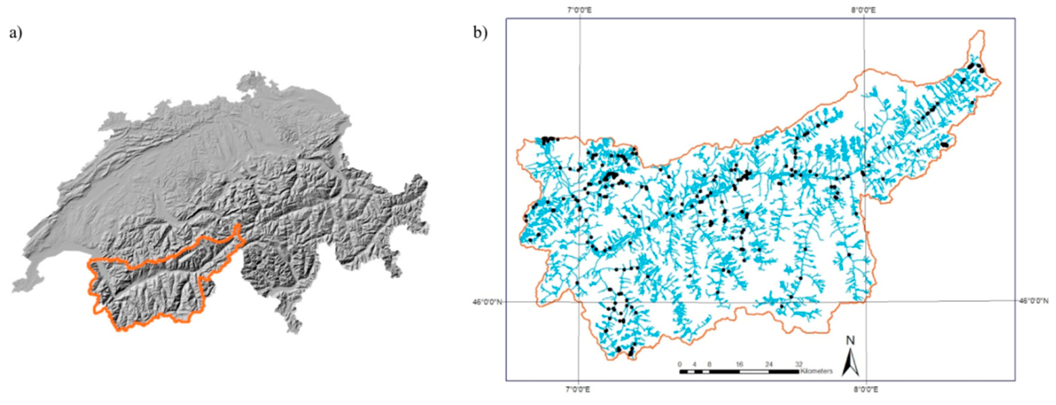
2.1. Study Area
2.2. Species Occurrence Data
2.3. Species Distribution Models (SDM)
2.3.1. Temporal and Spatial Scales of Environmental Variables
2.3.2. Environmental Predictors
2.3.3. Methods included in the Species Distribution Models (SDMs)
- -
- -
- -
2.4. Trait-Based Approach
2.4.1. Species Traits
2.4.2. Trait Analysis
3. Results
3.1. Species Distribution Models
3.1.1. Model Performance
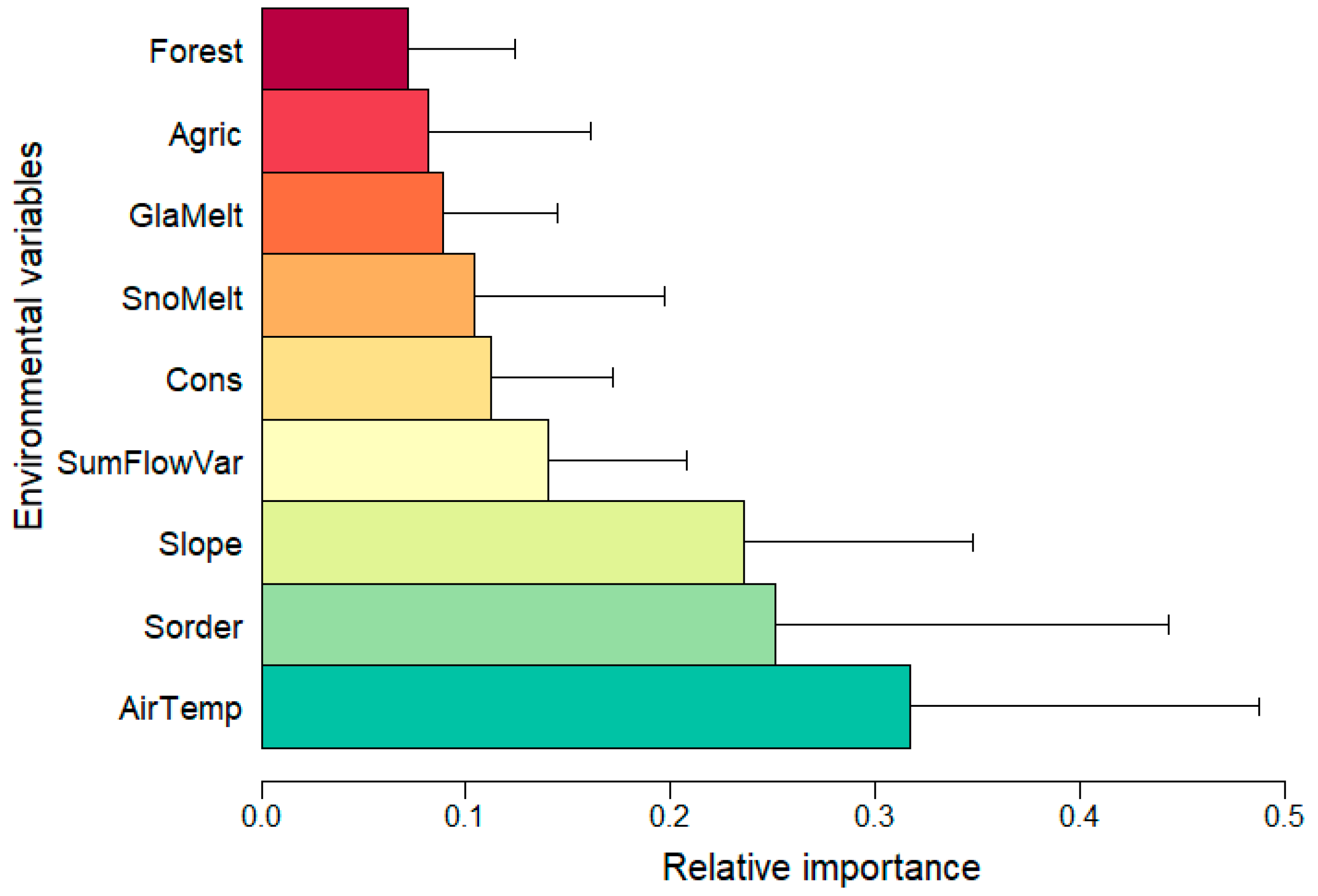
3.1.2. Contribution of the Variables
3.1.3. Assessing Species Vulnerability from SDMs
- -
- “Winners” (24 species): all the species of this group are potentially favoured by an increase in air temperature. Only 2 species in this group were mostly associated with stream upper reaches (stream order ≤ 5). Thirteen species occurred preferably at higher stream order (≥5) and they can be predicted to expand their distribution upstream under warming temperature.
- -
- “Losers” (27 species): this group contains species presenting either a bell-shaped response or a decreasing response to increasing air temperature. The latter occurred only in the case of the Plecoptera Rhabdiopteryx harperi. Fourteen species in this group showed a preference for low stream orders (≤ 5). These species should either show a contraction (those associated with the lowest stream orders) or an upstream shift of their range, making them vulnerable. In this group, five species associated with the higher stream order (≥5) and seven species with no definite longitudinal preference might be regarded as vulnerable depending on their ability to move upstream in the catchment.
- -
- Finally, a third group (not presented in Table 3) assembles twelve species that were not significantly related to air temperature in the SDMs.
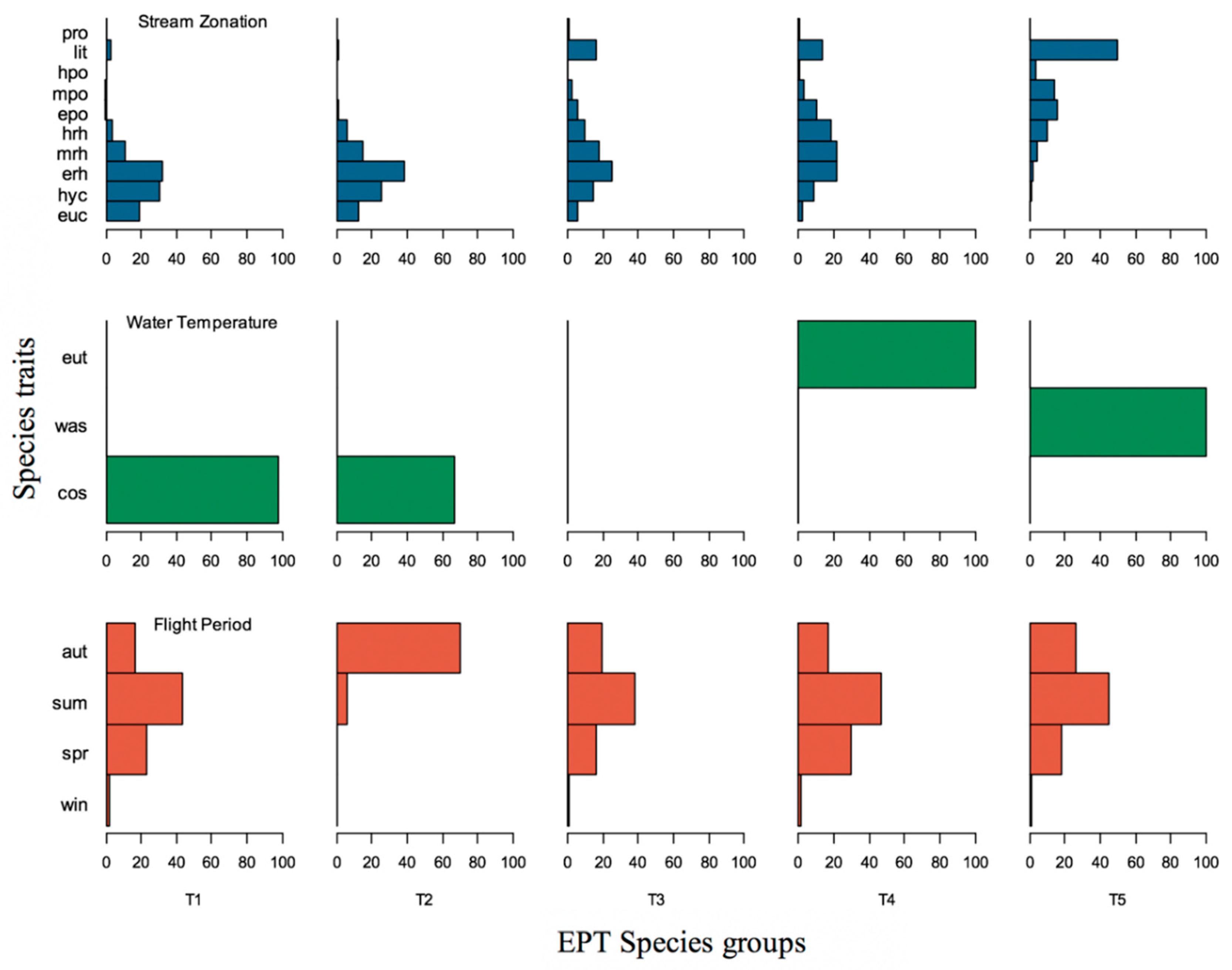
3.2. Trait-Based Approach
3.3. Confronting SDM and Trait Groupings
4. Discussion
4.1. Environmental Variables in the SDM
4.2. Can a Trait-Based Approach Supplement SDMs?
4.3. Winners and Losers
4.4. Conservation Perspectives
- -
- Four species were at the same time considered “Near Threatened” in the Swiss red list and identified as potential “losers” in both the SDM and trait analyses: Leuctra rauscheri (P) Nemoura sinuata (P), Siphonoperla montana (P), Cryptothrix nebulicola (T)
- -
- Fifteen species, among which are ten Plecoptera, do not currently have a threat status in Switzerland but were identified according to the trait and SDM analyses as being potential “losers” under climate change: Ecdyonurus picteti (E), Epeorus alpicola (E), Chloroperla susemicheli (P), Dictyogenus alpinum (P), Isoperla rivulorum (P), Leuctra braueri (P), Leuctra rosinae (P), Leuctra teriolensis (P), Perlodes intricatus (P), Protonemura brevistyla (P), Protonemura lateralis (P), Protonemura nimborum (P), Drusus discolor (T), Halesus rubricollis (T), Melampophylax melampus (T)
- -
- Thirteen species (among which only three Plecoptera) have no current threat status in Switzerland and were identified as potential “winners” under climate change by both methods: Baetis muticus (E), Baetis rhodani (E), Cloeon dipterum (E), Rhithrogena alpestris (E)m Rhithrogena hybrida (E), Brachyptera risi (P), Leuctra major (P), Protonemura intricata (P), Allogamus auricollis (T), Hydropsyche instabilis (T), Potamophylax cingulatus (T), Rhyacophila torrentium (T), Rhyacophila dorsalis (T)
- -
- Seventy-one species were considered as potential “losers” under climate change by the trait analysis (see Appendix D). Thirty-seven of them also had a threat status in the Swiss red list (including two of the three “Critically Endangered” species and three of the six “Endangered”). As no SDM were available in this set, particular attention should be paid to these species, including efforts to gather more precise information about their ecological requirements.
- -
- Twenty-two species with a threat status in Switzerland were not identified as potential losers, neither by the trait, nor by the SDM analyses. Some of them could even be considered as potential “winners” in the trait analysis (see Appendix D). This seems to indicate that these species are vulnerable because their habitat is generally under threat but potentially not because of climate change.
5. Conclusions
Author Contributions
Funding
Acknowledgments
Conflicts of Interest
Appendix A

| AirTemp | GlacArea | GlaMelt | SnoMelt | FlowVar | SumFlowVar | Mean | Low | Hispell | Base | Zero | Dure | Cons | Rise | Forest | Agric | SOrder | Alti | |
|---|---|---|---|---|---|---|---|---|---|---|---|---|---|---|---|---|---|---|
| AirTemp | ||||||||||||||||||
| GlacArea | −0.27 *** | |||||||||||||||||
| GlaMelt | −0.25 *** | 0.93 *** | ||||||||||||||||
| SnoMelt | −0.45 *** | 0.25 *** | 0.22 *** | |||||||||||||||
| FlowVar | 0.55 *** | 0.15 *** | 0.10 *** | −0.13 *** | ||||||||||||||
| SumFlowVar | 0.47 *** | 0.28 *** | 0.22 *** | 0.02 *** | 0.90 *** | |||||||||||||
| Mean | 0.52 *** | 0.04 *** | 0 | −0.19 *** | 0.85 *** | 0.78 *** | ||||||||||||
| Low | −0.34 *** | 0,43 *** | 0,48 *** | 0.34 *** | −0.22 *** | −0.03 *** | −0.25 *** | |||||||||||
| Hispell | 0.23 *** | −0.32 *** | −0.27 *** | −0.30 *** | 0 | −0.22 *** | −0.11 *** | −0.34 *** | ||||||||||
| Base | 0.50 *** | −0.31 *** | −0.29 *** | −0.28 *** | 0.40 *** | 0.32 *** | 0.44 *** | −0.53 *** | 0.22 *** | |||||||||
| Zero | −0.16 *** | 0.08 *** | 0.03 *** | −0.04 *** | −0.12 *** | −0.15 *** | −0.06 *** | −0.38 *** | −0.13 *** | −0.43 *** | ||||||||
| Dure | −0.06 *** | 0.25 *** | 0.22 *** | 0.32 *** | 0.25 *** | 0.35 *** | 0.25 *** | 0.04 *** | −0.66 *** | 0.28 *** | −0.08 *** | |||||||
| Cons | −0.25 *** | 0 | 0.01 | −0.09 *** | −0.38 *** | −0.38 *** | −0.20 *** | 0.18 *** | −0.08 *** | −0.66 *** | 0.48 *** | −0.46 *** | ||||||
| Rise | 0.45 *** | −0.18 *** | −0.16 *** | −0.12 *** | 0.47 *** | 0.38 *** | 0.29 *** | −0.05 *** | 0.45 *** | 0.55 *** | −0.72 *** | −0.16 *** | −0.53 *** | |||||
| Forest | 0.20 *** | −0.12 *** | −0.11 *** | −0.17 *** | 0.06 *** | 0.04 *** | 0.05 *** | −0.09 *** | 0.07 *** | 0.08 *** | −0.02 ** | −0.07 *** | −0.04 *** | 0.07 *** | ||||
| Agric | 0.19 *** | −0.07 *** | −0.08 *** | −0.13 *** | 0.11 *** | 0.09 *** | 0.10 *** | −0.06 *** | 0.03 *** | 0.08 *** | −0.04 *** | −0.03 *** | −0.03 *** | 0.10 *** | −0.08 *** | |||
| SOrder | 0.34 *** | 0.01 | 0 | −0.05 *** | 0.18 *** | 0.18 *** | 0.14 *** | −0.04 *** | 0.02 * | 0.09 *** | −0.04 *** | 0.03 *** | −0.08 *** | 0.10 *** | 0.04 *** | 0.03 *** | ||
| Alti | −0.97 *** | 0.29 *** | 0.28 *** | 0.38 *** | −0.54 *** | −0.48 *** | −0.52 *** | 0.34 *** | −0.23 *** | −0.51 *** | 0.18 *** | 0.05 *** | 0.27 *** | −0.47 *** | −0.19 *** | −0.19 *** | −0.37 *** | |
| Slope | −0.27 *** | −0.05 *** | −0.06 *** | 0.04 *** | −0.29 *** | −0.25 *** | −0.33 *** | 0.06 *** | 0.03 *** | −0.12 *** | 0 | −0.10 *** | 0.03 *** | −0.08 *** | 0.04 *** | −0.04 *** | −0.34 *** | 0.27 *** |
Appendix B
| Species | Order | Number of Occurrences | ANN | CTA | FDA | GAM | GBM | GLM | MARS | MAXENT | RF | Mean |
|---|---|---|---|---|---|---|---|---|---|---|---|---|
| Alainites muticus (Linnaeus, 1758) | E | 10 | 0.96 | 0.92 | 0.82 | 0.99 | NA | 0.99 | 0.93 | 0.79 | 0.99 | 0.92 |
| Allogamus auricollis (Pictet, 1834) | T | 50 | 0.95 | 0.91 | 0.85 | 0.86 | 0.88 | 0.83 | 0.90 | 0.85 | 0.98 | 0.89 |
| Allogamus hilaris (McLachlan, 1876) | T | 16 | 1.00 | 0.96 | 0.90 | 0.99 | NA | 0.90 | 0.99 | 0.68 | 1.00 | 0.92 |
| Allogamus mendax (McLachlan, 1876) | T | 13 | 0.97 | 0.90 | 0.81 | 0.98 | NA | 0.85 | 0.83 | 0.77 | 1.00 | 0.89 |
| Baetis alpinus (Pictet, 1843) | E | 173 | 0.87 | 0.86 | 0.84 | 0.84 | 0.88 | 0.83 | 0.85 | 0.88 | 0.98 | 0.87 |
| Baetis melanonyx (Pictet, 1843) | E | 23 | 0.95 | 0.95 | 0.92 | 0.94 | 0.93 | 0.94 | 0.95 | 0.94 | 0.98 | 0.94 |
| Baetis rhodani (Pictet, 1843) | E | 69 | 0.94 | 0.91 | 0.86 | 0.85 | 0.90 | 0.85 | 0.89 | 0.89 | 0.98 | 0.90 |
| Brachyptera risi (Morton, 1896) | p | 13 | 0.98 | 0.94 | 0.88 | 0.98 | NA | 0.98 | 0.96 | 0.88 | 0.99 | 0.95 |
| Capnioneura nemuroides Ris, 1905 | p | 13 | 0.99 | 0.96 | 0.96 | 0.99 | NA | 0.99 | 0.98 | 0.94 | 0.99 | 0.98 |
| Chloroperla susemicheli Zwick, 1967 | p | 27 | 0.97 | 0.93 | 0.87 | 0.92 | 0.89 | 0.87 | 0.93 | 0.90 | 0.98 | 0.92 |
| Cloeon dipterum (Linnaeus, 1761) | E | 11 | 0.99 | 0.95 | 0.93 | 0.99 | NA | 0.99 | 0.98 | 0.93 | 0.98 | 0.97 |
| Cryptothrix nebulicola McLachlan, 1867 | T | 14 | 0.93 | 0.92 | 0.80 | 0.96 | NA | 0.93 | 0.89 | 0.83 | 0.99 | 0.90 |
| Dictyogenus alpinus (Pictet, 1841) | P | 43 | 0.93 | 0.93 | 0.86 | 0.89 | 0.90 | 0.89 | 0.90 | 0.90 | 0.98 | 0.91 |
| Drusus biguttatus (Pictet, 1834) | T | 29 | 0.91 | 0.91 | 0.82 | 0.85 | 0.86 | 0.87 | 0.91 | 0.89 | 0.98 | 0.89 |
| Drusus discolor (Rambur, 1842) | T | 35 | 0.92 | 0.92 | 0.77 | 0.82 | 0.87 | 0.76 | 0.84 | 0.82 | 0.99 | 0.86 |
| Ecdyonurus helveticus Eaton, 1883 | E | 42 | 0.93 | 0.91 | 0.85 | 0.86 | 0.88 | 0.85 | 0.90 | 0.88 | 0.98 | 0.89 |
| Ecdyonurus parahelveticus Hefti, Tomka & Zurwerra, 1986 | E | 11 | 0.97 | 0.94 | 0.97 | 0.99 | NA | 0.99 | 0.98 | 0.91 | 0.99 | 0.97 |
| Ecdyonurus picteti (Meyer-Dür, 1864) | E | 53 | 0.91 | 0.89 | 0.87 | 0.89 | 0.89 | 0.89 | 0.89 | 0.89 | 0.98 | 0.90 |
| Ecdyonurus venosus (Fabricius, 1775) | E | 12 | 0.99 | 0.99 | 0.98 | 1.00 | NA | 1.00 | 1.00 | 0.98 | 1.00 | 0.99 |
| Epeorus alpicola (Eaton, 1871) | E | 46 | 0.91 | 0.93 | 0.83 | 0.85 | 0.90 | 0.86 | 0.89 | 0.87 | 0.98 | 0.89 |
| Halesus rubricolis (Pictet, 1834) | T | 26 | 0.95 | 0.91 | 0.75 | 0.85 | 0.84 | 0.80 | 0.92 | 0.82 | 0.99 | 0.87 |
| Hydropsyche instabilis (Curtis, 1834) | T | 10 | 0.97 | 0.92 | 0.90 | 0.99 | NA | 0.98 | 0.95 | 0.90 | 0.98 | 0.95 |
| Isoperla ivolorum (Pictet, 1841) | P | 46 | 0.93 | 0.92 | 0.85 | 0.85 | 0.90 | 0.86 | 0.90 | 0.88 | 0.98 | 0.90 |
| Leucra braueri Kempny, 1898 | P | 13 | 0.97 | 0.96 | 0.94 | 0.99 | NA | 0.99 | 0.98 | 0.91 | 0.99 | 0.96 |
| Leuctra cingulata Kempny, 1899 | P | 16 | 0.98 | 0.96 | 0.96 | 0.99 | NA | 0.99 | 0.98 | 0.95 | 0.99 | 0.97 |
| Leuctra biermis Kempny, 1899 | P | 35 | 0.91 | 0.91 | 0.85 | 0.85 | 0.89 | 0.87 | 0.90 | 0.88 | 0.98 | 0.89 |
| Leuctra major Brinck, 1949 | P | 11 | 0.95 | 0.92 | 0.87 | 0.92 | NA | 0.97 | 0.94 | 0.82 | 0.99 | 0.92 |
| Leuctra moselyi Morton, 1929 | P | 13 | 0.95 | 0.91 | 0.85 | 0.96 | NA | 0.95 | 0.94 | 0.84 | 0.99 | 0.92 |
| Leuctra rauscheri Aubert, 1957 | P | 20 | 0.90 | 0.91 | 0.83 | 0.84 | 0.85 | 0.85 | 0.88 | 0.89 | 0.99 | 0.88 |
| Leuctra rosinae Kempny, 1900 | P | 21 | 0.93 | 0.95 | 0.84 | 0.92 | 0.82 | 0.86 | 0.91 | 0.88 | 0.98 | 0.90 |
| Leuctra teriolensis Kempny, 1900 | P | 15 | 0.94 | 0.95 | 0.87 | 0.94 | NA | 0.91 | 0.93 | 0.80 | 0.99 | 0.92 |
| Melampophylax melampus (McLachlan, 1876) | T | 14 | 0.98 | 0.95 | 0.90 | 0.99 | NA | 0.99 | 0.97 | 0.84 | 0.99 | 0.95 |
| Metanoea flavipennis (Pictet, 1834) | T | 16 | 0.98 | 0.96 | 0.85 | 0.97 | NA | 0.92 | 0.96 | 0.76 | 0.99 | 0.92 |
| Nemoura mortoni Ris, 1902 | P | 43 | 0.90 | 0.91 | 0.85 | 0.88 | 0.89 | 0.86 | 0.88 | 0.88 | 0.98 | 0.89 |
| Nemoura obtusa Ris, 1902 | P | 12 | 0.98 | 0.96 | 0.90 | 0.99 | NA | 0.99 | 0.97 | 0.89 | 0.99 | 0.96 |
| Nemoura sinuata Ris, 1902 | P | IS | 0.93 | 0.90 | 0.76 | 0.91 | 0.73 | 0.87 | 0.90 | 0.66 | 0.99 | 0.85 |
| Nemurella pictetii Klapálek,1900 | P | 23 | 0.95 | 0.95 | 0.90 | 0.94 | 0.90 | 0.94 | 0.95 | 0.94 | 0.99 | 0.94 |
| Perla grandis Rambur, 1842 | P | 13 | 0.96 | 0.94 | 0.86 | 0.98 | NA | 0.98 | 0.97 | 0.88 | 0.99 | 0.94 |
| Perlodes intricatus (Pictet, 1841) | P | 25 | 0.95 | 0.94 | 0.91 | 0.94 | 0.91 | 0.92 | 0.93 | 0.92 | 0.98 | 0.93 |
| Philopotamus ludificatus McLachlan, 1878 | T | 29 | 0.93 | 0.94 | 0.83 | 0.90 | 0.86 | 0.85 | 0.92 | 0.88 | 0.99 | 0.90 |
| Plectrocnemia geniculata McLachlan, 1871 | T | 14 | 0.99 | 0.97 | 0.90 | 0.99 | NA | 0.99 | 0.99 | 0.83 | 1.00 | 0.96 |
| Potamophylax cingulatus (Stephens, 1837) | T | 28 | 0.98 | 0.94 | 0.86 | 0.93 | 0.90 | 0.91 | 0.95 | 0.79 | 0.99 | 0.92 |
| Protonemura brevistyla (Ris, 1902) | P | 3! | 0.94 | 0.94 | 0.87 | 0.92 | 0.90 | 0.91 | 0.91 | 0.92 | 0.99 | 0.92 |
| Protonemura intricata (Ris, 1902) | P | 10 | 0.95 | 0.91 | 0.86 | 0.96 | NA | 0.99 | 0.93 | 0.86 | 0.99 | 0.93 |
| Protonemura lateralis (Pictet, 1836) | P | 55 | 0.91 | 0.91 | 0.83 | 0.86 | 0.88 | 0.84 | 0.87 | 0.88 | 0.98 | 0.89 |
| Protonemura nimborella Mosely, 1930 | P | 10 | 0.93 | 0.95 | 0.88 | 0.96 | NA | 0.98 | 0.93 | 0.78 | 0.99 | 0.92 |
| Protonemura nimborum (Ris, 1902) | P | 30 | 0.94 | 0.92 | 0.87 | 0.91 | 0.88 | 0.90 | 0.92 | 0.90 | 0.98 | 0.91 |
| Protonemura nitida (Pictet, 1835) | P | 45 | 0.92 | 0.91 | 0.85 | 0.86 | 0.89 | 0.85 | 0.91 | 0.87 | 0.98 | 0.89 |
| Protonemura risi (Jacobson & Bianchi, 1905) | P | 10 | 0.99 | 0.97 | 0.98 | 0.99 | NA | 0.99 | 0.99 | 0.94 | 0.99 | 0.98 |
| Rhabdiopteryx haperi Vinçon & Muranyi, 2008 | P | 13 | 0.99 | 0.98 | 0.92 | 0.99 | NA | 0.99 | 0.97 | 0.94 | 0.99 | 0.97 |
| Rhabdiopteryx neglecta (Albarda, 1889) | P | 16 | 0.93 | 0.90 | 0.83 | 0.92 | NA | 0.88 | 0.87 | 0.82 | 0.98 | 0.89 |
| Rhithrogena alpestris Eaton, 1885 | E | 27 | 0.94 | 0.91 | 0.88 | 0.92 | 0.89 | 0.91 | 0.92 | 0.90 | 0.98 | 0.92 |
| Rhithrogena degrangei Sowa, 1969 | E | 23 | 0.95 | 0.94 | 0.91 | 0.94 | 0.92 | 0.93 | 0.94 | 0.94 | 0.97 | 0.94 |
| Rhithrogena hybrida Eaton, 1885 | E | 35 | 0.96 | 0.95 | 0.91 | 0.94 | 0.93 | 0.93 | 0.94 | 0.94 | 0.99 | 0.94 |
| Rhithrogena loyolaea Navás, 1922 | E | 45 | 0.91 | 0.96 | 0.80 | 0.85 | 0.91 | 0.82 | 0.85 | 0.86 | 0.99 | 0.88 |
| Rhithrogena nivata (Eaton, 1871) | E | 15 | 0.98 | 0.97 | 0.93 | 0.99 | NA | 0.98 | 0.97 | 0.93 | 0.99 | 0.97 |
| Rhyacophila dorsalis (Curtis, 1834) | T | 12 | 0.99 | 0.97 | 0.95 | 0.99 | NA | 0.99 | 0.99 | 0.95 | 0.99 | 0.98 |
| Rhyacophila intermedia McLachlan, 1868 | T | 37 | 0.89 | 0.96 | 0.83 | 0.87 | 0.88 | 0.83 | 0.90 | 0.87 | 0.99 | 0.89 |
| Rhyacophila pubescens Pictet, 1834 | T | 12 | 0.97 | 0.96 | 0.91 | 0.99 | NA | 0.99 | 0.96 | 0.87 | 0.99 | 0.95 |
| Rhyacophila torrentium Pictet, 1834 | T | 30 | 0.92 | 0.90 | 0.86 | 0.88 | 0.88 | 0.88 | 0.92 | 0.89 | 0.98 | 0.90 |
| Rhyacophila tristis Pictet, 1834 | T | 11 | 0.94 | 0.95 | 0.89 | 0.99 | NA | 0.97 | 0.97 | 0.79 | 0.99 | 0.94 |
| Rhyacophila vulgaris Pictet, 1834 | T | 41 | 0.92 | 0.94 | 0.83 | 0.85 | 0.88 | 0.83 | 0.92 | 0.87 | 0.99 | 0.89 |
| Siphonoperla montaba (Pictet, 1841) | P | 15 | 0.97 | 0.96 | 0.93 | 0.99 | NA | 0.98 | 0.96 | 0.92 | 0.99 | 0.96 |
Appendix C
| Species | Order | Air Temp | Sorder | Slope | Sun FlowVar | Cons | Sno Melt | Gla Melt | Agric | Forest |
|---|---|---|---|---|---|---|---|---|---|---|
| Alainites muticus (Linnaeus, 1758) | E | 0.61 * | 0.13 | 0.21 | 0.09 | 0.1 | 0.08 | 0.09 | 0.06 | 0.15 |
| Allogamus auricollis (Pictet, 1834) | T | 0.67 * | 0.15 | 0.28 | 0.17 | 0.2 | 0.11 | 0.11 | 0.15 | 0.13 |
| Allogamus hilaris (McLachlan, 1876) | T | 0.32 * | 0.17 | 0.28 | 0.18 | 0.18 | 0.11 | 0.21 | 0.31 | 0.16 |
| Allogamus mendax (McLachlan, 1876) | T | 0.25 | 0.14 | 0.26 | 0.17 | 0.19 | 0.18 | 0.22 | 0.13 | 0.32 * |
| Baetis alpinus (Pictet, 1843) | E | 0.17 | 0.57 * | 0.13 | 0.07 | 0.04 | 0.03 | 0.1 | 0.02 | 0.02 |
| Baetis melanonyx (Pictet, 1843) | E | 0.34 * | 0.2 | 0.28 | 0.15 | 0.1 | 0.04 | 0.15 | 0.08 | 0.03 |
| Baetis rhodani (Pictet, 1843) | E | 0.51 * | 0.38 | 0.28 | 0.19 | 0.17 | 0.12 | 0.14 | 0.14 | 0.14 |
| Brachyptera risi (Morton, 1896) | P | 0.34 * | 0.22 | 0.33 | 0.20 | 0.12 | 0.25 | 0.15 | 0.07 | 0.1 |
| Capnioneura nemuroides Ris, 1905 | P | 0.26 | 0.11 | 031 * | 0.24 | 0.16 | 0.13 | 0.16 | 0.06 | 0.05 |
| Chloroperla susemicheli Zwick, 1967 | P | 0.33 | 0.41 * | 0.34 | 0.21 | 0.23 | 0.13 | 0.13 | 0.15 | 0.13 |
| Cloeon dipterum (Linnaeus, 1761) | E | 0.19 | 0.06 | 0.48 * | 0.27 | 0.12 | 0.04 | 0.03 | 0.03 | 0.13 |
| Cryptothrix nebulicola McLachlan, 1867 | T | 0.15 | 0.62 * | 0.16 | 0.1 | 0.11 | 0.07 | 0.13 | 0.05 | 0.08 |
| Dictyogenus alpinus (Pictet, 1841) | P | 0.15 | 0.48 * | 0.28 | 0.07 | 0.05 | 0.09 | 0.04 | 0.04 | 0.04 |
| Drusus biguttatus (Pictet, 1834) | T | 0.26 | 0.39 * | 0.17 | 0.11 | 0.12 | 0.08 | 0.05 | 0.06 | 0.04 |
| Drusus discolor (Rambur, 1842) | T | 0.15 | 0.44 * | 0.15 | 0.11 | 0.2 | 0.07 | 0.08 | 0.04 | 0.04 |
| Ecdyonurus helveticus Eaton, 1883 | E | 0.58 * | 0.13 | 0.19 | 0.1 | 0.04 | 0.03 | 0.06 | 0.08 | 0.05 |
| Ecdyonurus parahelveticus Hefti, Tomka & Zurwerra, 1986 | E | 0.24 | 0.05 | 0.19 | 0.28 * | 0.11 | 0.04 | 0.25 | 0.12 | 0.06 |
| Ecdyonurus picteti (Meyer-Dür, 1864) | E | 0.14 | 0.63 * | 0.16 | 0.06 | 0.04 | 0.03 | 0.03 | 0.02 | 0.03 |
| Ecdyonurus venosus (Fabricius, 1775) | E | 0.21 | 0.51 * | 0.08 | 0.07 | 0.07 | 0.18 | 0.1 | 0.02 | 0.05 |
| Epeorus alpicola (Eaton, 1871) | E | 0.33 * | 0.29 | 0.12 | 0.12 | 0.05 | 0.05 | 0.13 | 0.07 | 0.05 |
| Halesus rubricolis (Pictet, 1834) | T | 0.32 * | 0.11 | 0.16 | 0.1 | 0.09 | 0.06 | 0.06 | 0.27 | 0.14 |
| Hydropsyche instabilis (Curtis, 1834) | T | 0.15 * | 0.08 | 0.1 | 0.15 | 0.07 | 0.07 | 0.04 | 0.01 | 0.05 |
| Isoperla ivolorum (Pictet, 1841) | P | 0.51 * | 0.1 | 0.31 | 0.11 | 0.07 | 0.05 | 0.04 | 0.05 | 0.03 |
| Leucra braueri Kempny, 1898 | P | 0.32 * | 0.07 | 0.18 | 0.17 | 0.29 | 0.17 | 0.09 | 0.02 | 0.04 |
| Leuctra cingulata Kempny, 1899 | P | 0.39 * | 0.05 | 0.28 | 0.2 | 0.2 | 0.03 | 0.15 | 0.03 | 0.02 |
| Leuctra biermis Kempny, 1899 | P | 0.33 * | 032 | 0.21 | 0.08 | 0.07 | 0.03 | 0.04 | 0.1 | 0.06 |
| Leuctra major Brinck, 1949 | P | 0.26 | 0.23 | 0.41 * | 0.12 | 0.07 | 0.1 | 0.05 | 0.05 | 0.07 |
| Leuctra moselyi Morton, 1929 | P | 0.16 | 0.23 | 0.33 * | 0.21 | 0.21 | 0.06 | 0.09 | 0.07 | 0.08 |
| Leuctra rauscheri Aubert, 1957 | P | 0.22 | 0.15 | 0.43 * | 0.13 | 0.16 | 0.09 | 0.06 | 0.03 | 0.05 |
| Leuctra rosinae Kempny, 1900 | P | 0.2 | 0.1 | 0.32 * | 0.22 | 0.14 | 0.2 | 0.07 | 0.06 | 0.07 |
| Leuctra teriolensis Kempny, 1900 | P | 0.17 | 0.21 | 0.26 * | 0.15 | 0.15 | 0.18 | 0.05 | 0.06 | 0.18 |
| Melampophylax melampus (McLachlan, 1876) | T | 0.72 * | 0.11 | 0.15 | 0.11 | 0.1 | 0.06 | 0.08 | 0.1 | 0.06 |
| Metanoea flavipennis (Pictet, 1834) | T | 0.13 | 0.31 * | 0.23 | 0.15 | 0.1 | 0.21 | 0.15 | 0.08 | 0.11 |
| Nemoura mortoni Ris, 1902 | P | 0.13 | 0.58 * | 0.2 | 0.08 | 0.07 | 003 | 0.13 | 0.03 | 0.04 |
| Nemoura obtusa Ris, 1902 | P | 0.15 | 0.08 | 0.3 | 0.21 | 0.13 | 0.46 * | 0.03 | 0.04 | 0.08 |
| Nemoura sinuata Ris, 1902 | P | 0.33 * | 0.1 | 0.21 | 021 | 0.25 | 0.13 | 0.18 | 0.08 | 0.12 |
| Nemurella pictetii Klapálek,1900 | P | 0.26 | 0.12 | 0.35 * | 0.13 | 0.07 | 0.15 | 0.08 | 0.04 | 0.2 |
| Perla grandis Rambur, 1842 | P | 0.17 | 0.43 * | 0.17 | 0.14 | 0.07 | 0.2 | 0.17 | 0.03 | 0.05 |
| Perlodes intricatus (Pictet, 1841) | P | 0.31 | 0.06 | 0.57 * | 0.13 | 0.09 | 0.04 | 0.04 | 0.06 | 0.04 |
| Philopotamus ludificatus McLachlan, 1878 | T | 0.57 * | 0.06 | 0.21 | 0.11 | 0.1 | 0.06 | 0.05 | 0.1 | 0.03 |
| Plectrocnemia geniculata McLachlan, 1871 | T | 0.48 * | 0.09 | 0.17 | 0.12 | 0.1 | 0.04 | 0.03 | 0.36 | 0.08 |
| Potamophylax cingulatus (Stephens, 1837) | T | 0.42 * | 0.11 | 0.14 | 0.09 | 0.09 | 0.01 | 0.03 | 0.22 | 0.08 |
| Protonemura brevistyla (Ris, 1902) | P | 0.13 | 0.39 * | 0.19 | 0.09 | 0.07 | 0.22 | 0.04 | 0.03 | 0.09 |
| Protonemura intricata (Ris, 1902) | P | 0.56 * | 0.08 | 0.13 | 0.13 | 0.09 | 0.13 | 0.19 | 0.06 | 0.07 |
| Protonemura lateralis (Pictet, 1836) | P | 0.22 | 0.24 | 0.39 | 0.09 | 0.07 | 0.15 | 0.07 | 0.02 | 0.04 |
| Protonemura nimborella Mosely, 1930 | P | 0.25 | 0.2 | 0.27 * | 0.16 | 0.22 | 0.1 | 0.16 | 0.06 | 0.08 |
| Protonemura nimborum (Ris, 1902) | P | 0.4 * | 032 | 0.23 | 0.08 | 0.06 | 0.05 | 0.03 | 0.03 | 0.04 |
| Protonemura nitida (Pictet, 1835) | P | 0.45 * | 0.27 | 0.23 | 0.09 | 0.06 | 0.03 | 0.03 | 0.04 | 0.02 |
| Protonemura risi (Jacobson & Bianchi, 1905) | P | 0.19 | 0.06 | 0.08 | 0.45 * | 0.25 | 0.04 | 0.1 | 0.04 | 0.03 |
| Rhabdiopteryx haperi Vinçon & Muranyi, 2008 | P | 0.21 | 0.19 | 0.21 | 0.1 | 0.08 | 0.53 * | 0.05 | 0.05 | 0.05 |
| Rhabdiopteryx neglecta (Albarda, 1889) | P | 0.13 | 0.61 * | 0.17 | 0.1 | 0.08 | 0.06 | 0.05 | 0.04 | 0.06 |
| Rhithrogena alpestris Eaton, 1885 | E | 0.25 | 0.61 * | 0.16 | 0.06 | 0.05 | 0.04 | 0.04 | 0.02 | 0.03 |
| Rhithrogena degrangei Sowa, 1969 | E | 0.09 | 0.76 * | 0.1 | 0.06 | 0.04 | 0.04 | 0.05 | 0.02 | 0.03 |
| Rhithrogena hybrida Eaton, 1885 | E | 0.42 * | 0.32 | 0.17 | 0.09 | 0.04 | 0.03 | 0.11 | 0.02 | 0.03 |
| Rhithrogena loyolaea Navás, 1922 | E | 0.16 | 0.24 | 0.23 | 0.27 * | 0.08 | 0.19 | 0.08 | 0.02 | 0.05 |
| Rhithrogena nivata (Eaton, 1871) | E | 0.2 | 0.71 * | 0.13 | 0.13 | 0.06 | 0.08 | 0.04 | 0.03 | 0.04 |
| Rhyacophila dorsalis (Curtis, 1834) | T | 0.72 * | 0.07 | 0.06 | 0.14 | 0.09 | 0.06 | 0.04 | 0.08 | 0.06 |
| Rhyacophila intermedia McLachlan, 1868 | T | 0.25 | 0.12 | 0.23 | 0.08 | 0.1 | 0.07 | 0.18 | 0.29 * | 0.06 |
| Rhyacophila pubescens Pictet, 1834 | T | 0.6 * | 0.09 | 0.17 | 0.12 | 0.11 | 0.05 | 0.07 | 0.26 | 0.06 |
| Rhyacophila torrentium Pictet, 1834 | T | 0.18 | 0.43 * | 0.1 | 0.19 | 0.14 | 0.03 | 0.03 | 0.09 | 0.04 |
| Rhyacophila tristis Pictet, 1834 | T | 0.51 * | 0.08 | 0.34 | 0.09 | 0.08 | 0.17 | 0.04 | 0.03 | 0.06 |
| Rhyacophila vulgaris Pictet, 1834 | T | 0.32 * | 0.08 | 0.24 | 0.1 | 0.12 | 0.03 | 0.06 | 0.25 | 0.06 |
| Siphonoperla montaba (Pictet, 1841) | P | 0.26 | 0.16 | 0.6 * | 0.15 | 0.06 | 0.12 | 0.05 | 0.03 | 0.06 |
Appendix D
| Order | trait Group | SDM Group | Swiss Red List | |
|---|---|---|---|---|
| Baetis alpinus | E | T1 | “winner” | |
| Caenis robusta | E | T1 | NT | |
| Ecdyonurus alpinus | E | T1 | NT | |
| Ecdyonurus picteti | E | T1 | “loser” | |
| Ecdyonurus zelleri | E | T1 | ||
| Epeorus alpicola | E | T1 | “loser” | |
| Rhithrogena gratianopolitana | E | T1 | ||
| Rhithrogena loyolaea | E | T1 | NC | |
| Rhithrogena puthzi | E | T1 | ||
| Caenis lactea | E | T3 | VU | |
| Rhithrogena nivata | E | T3 | NC | NT |
| Baetis melanonyx | E | T4 | “loser” | NT |
| Baetis muticus | E | T4 | “winner” | |
| Baetis rhodani | E | T4 | “winner” | |
| Baetis vernus | E | T4 | ||
| Caenis luctuosa | E | T4 | ||
| Caenis macrura | E | T4 | ||
| Cloeon dipterum | E | T4 | “winner” | |
| Ecdyonurus helveticus | E | T4 | “loser” | |
| Ecdyonurus parahelveticus | E | T4 | NC | VU |
| Ecdyonurus venosus | E | T4 | ||
| Epeorus assimilis | E | T4 | ||
| Habroleptoides auberti | E | T4 | ||
| Rhithrogena alpestris | E | T4 | “winner” | |
| Rhithrogena degrangei | E | T4 | NC | |
| Rhithrogena grischuna | E | T4 | NT | |
| Rhithrogena hybrida | E | T4 | “winner” | |
| Rhithrogena picteti | E | T4 | ||
| Rhithrogena semicolorata | E | T4 | ||
| Serratella ignita | E | T4 | ||
| Caenis horaria | E | T5 | ||
| Cloeon simile | E | T5 | ||
| Amphinemura triangularis | P | T1 | ||
| Capnia nigra | P | T1 | ||
| Chloroperla susemicheli | P | T1 | “loser” | |
| Chloroperla tripunctata | P | T1 | ||
| Dictyogenus alpinum | P | T1 | “loser” | |
| Dictyogenus fontium | P | T1 | NT | |
| Isoperla rivulorum | P | T1 | “loser” | |
| Leuctra alpina | P | T1 | ||
| Leuctra armata | P | T1 | NT | |
| Leuctra aurita | P | T1 | NT | |
| Leuctra braueri | P | T1 | “loser” | |
| Leuctra cingulata | P | T1 | NC | |
| Leuctra handlirschi | P | T1 | ||
| Leuctra leptogaster | P | T1 | ||
| Leuctra moselyi | P | T1 | NC | |
| Leuctra niveola | P | T1 | VU | |
| Leuctra pseudosignifera | P | T1 | NT | |
| Leuctra rauscheri | P | T1 | “loser” | NT |
| Leuctra ravizzai | P | T1 | CR | |
| Leuctra rosinae | P | T1 | “loser” | |
| Leuctra subalpina | P | T1 | NT | |
| Leuctra teriolensis | P | T1 | “loser” | |
| Nemoura marginata | P | T1 | ||
| Nemoura minima | P | T1 | NT | |
| Nemoura mortoni | P | T1 | NC | |
| Nemoura obtusa | P | T1 | NC | NT |
| Nemoura sinuata | P | T1 | “loser” | NT |
| Perla grandis | P | T1 | “winner” | |
| Perlodes intricatus | P | T1 | “loser” | |
| Protonemura algovia | P | T1 | VU | |
| Protonemura brevistyla | P | T1 | “loser” | |
| Protonemura lateralis | P | T1 | “loser” | |
| Protonemura nimborella | P | T1 | “winner” | VU |
| Protonemura praecox | P | T1 | ||
| Protonemura risi | P | T1 | NC | |
| Rhabdiopteryx alpina | P | T1 | NT | |
| Rhabdiopteryx neglecta | P | T1 | NC | |
| Siphonoperla montana | P | T1 | “loser” | NT |
| Siphonoperla torrentium | P | T1 | ||
| Taeniopteryx kuehtreiberi | P | T1 | ||
| Capnia vidua | P | T2 | NT | |
| Leuctra autumnalis | P | T2 | VU | |
| Leuctra schmidi | P | T2 | EN | |
| Protonemura nimborum | P | T2 | “loser” | |
| Capnioneura nemuroides | P | T3 | NC | |
| Brachyptera risi | P | T4 | “winner” | |
| Isoperla grammatica | P | T4 | ||
| Leuctra hexacantha | P | T4 | VU | |
| Leuctra inermis | P | T4 | “loser” | |
| Leuctra major | P | T4 | “winner” | |
| Leuctra nigra | P | T4 | ||
| Nemoura cinerea | P | T4 | ||
| Nemurella pictetii | P | T4 | “loser” | |
| Perlodes microcephalus | P | T4 | ||
| Protonemura intricata | P | T4 | “winner” | |
| Protonemura nitida | P | T4 | “loser” | |
| Acrophylax zerberus | T | T1 | VU | |
| Agapetus fuscipes | T | T1 | ||
| Allogamus hilaris | T | T1 | “winner” | |
| Anisogamus difformis | T | T1 | VU | |
| Apatania fimbriata | T | T1 | EN | |
| Cryptothrix nebulicola | T | T1 | “loser” | NT |
| Drusus alpinus | T | T1 | EN | |
| Drusus annulatus | T | T1 | ||
| Drusus chrysotus | T | T1 | NT | |
| Drusus discolor | T | T1 | “loser” | |
| Drusus melanchaetes | T | T1 | VU | |
| Drusus monticola | T | T1 | NT | |
| Drusus muelleri | T | T1 | VU | |
| Drusus nigrescens | T | T1 | VU | |
| Drusus trifidus | T | T1 | NT | |
| Ernodes vicinus | T | T1 | NT | |
| Glossosoma conformis | T | T1 | ||
| Halesus rubricollis | T | T1 | “loser” | |
| Hydropsyche tenuis | T | T1 | ||
| Limnephilus coenosus | T | T1 | NT | |
| Limnephilus extricatus | T | T1 | ||
| Limnephilus ignavus | T | T1 | ||
| Lithax niger | T | T1 | ||
| Plectrocnemia brevis | T | T1 | NT | |
| Pseudopsilopteryx zimmeri | T | T1 | ||
| Ptilocolepus granulatus | T | T1 | NT | |
| Rhadicoleptus ucenorum | T | T1 | CR | |
| Rhyacophila glareosa | T | T1 | NT | |
| Rhyacophila intermedia | T | T1 | “winner” | |
| Rhyacophila laevis | T | T1 | VU | |
| Rhyacophila pubescens | T | T1 | “winner” | |
| Rhyacophila stigmatica | T | T1 | VU | |
| Rhyacophila tristis | T | T1 | “winner” | |
| Tinodes unicolor | T | T1 | ||
| Tinodes zelleri | T | T1 | VU | |
| Wormaldia copiosa | T | T1 | ||
| Allogamus mendax | T | T2 | “winner” | NT |
| Allogamus uncatus | T | T2 | ||
| Consorophylax consors | T | T2 | NT | |
| Limnephilus hirsutus | T | T2 | NT | |
| Melampophylax melampus | T | T2 | “loser” | |
| Philopotamus variegatus | T | T2 | ||
| Plectrocnemia conspersa | T | T2 | ||
| Plectrocnemia geniculata | T | T2 | “winner” | NT |
| Rhyacophila vulgaris | T | T2 | “winner” | |
| Tinodes dives | T | T2 | ||
| Wormaldia occipitalis | T | T2 | ||
| Athripsodes cinereus | T | T3 | ||
| Drusus biguttatus | T | T3 | “loser” | |
| Glossosoma boltoni | T | T3 | ||
| Hydropsyche dinarica | T | T3 | ||
| Hydropsyche doehleri | T | T3 | EN | |
| Hydropsyche incognita | T | T3 | ||
| Hydropsyche instabilis | T | T3 | “winner” | |
| Hydroptila forcipata | T | T3 | ||
| Hydroptila vectis | T | T3 | ||
| Limnephilus binotatus | T | T3 | VU | |
| Limnephilus bipunctatus | T | T3 | EN | |
| Limnephilus decipiens | T | T3 | ||
| Limnephilus helveticus | T | T3 | VU | |
| Limnephilus italicus | T | T3 | VU | |
| Metanoea flavipennis | T | T3 | NC | NT |
| Micropterna nycterobia | T | T3 | NT | |
| Micropterna sequax | T | T3 | ||
| Micropterna testacea | T | T3 | ||
| Odontocerum albicorne | T | T3 | ||
| Parachiona picicornis | T | T3 | NT | |
| Philopotamus ludificatus | T | T3 | “loser” | |
| Potamophylax cingulatus | T | T3 | “winner” | |
| Potamophylax latipennis | T | T3 | ||
| Potamophylax nigricornis | T | T3 | NT | |
| Rhyacophila praemorsa | T | T3 | VU | |
| Rhyacophila simulatrix | T | T3 | CR | |
| Rhyacophila torrentium | T | T3 | “winner” | |
| Stenophylax mitis | T | T3 | ||
| Agrypnia pagetana | T | T4 | ||
| Agrypnia varia | T | T4 | ||
| Allogamus auricollis | T | T4 | “winner” | |
| Ceraclea dissimilis | T | T4 | ||
| Chaetopteryx villosa | T | T4 | ||
| Halesus digitatus | T | T4 | ||
| Halesus radiatus | T | T4 | ||
| Lepidostoma hirtum | T | T4 | ||
| Limnephilus lunatus | T | T4 | ||
| Lype phaeopa | T | T4 | ||
| Phryganea bipunctata | T | T4 | NT | |
| Psychomyia pusilla | T | T4 | ||
| Rhyacophila dorsalis | T | T4 | “winner” | |
| Setodes argentipunctellus | T | T4 | ||
| Silo nigricornis | T | T4 | ||
| Trichostegia minor | T | T4 | VU | |
| Agraylea multipunctata | T | T5 | ||
| Agraylea sexmaculata | T | T5 | ||
| Anabolia nervosa | T | T5 | ||
| Athripsodes aterrimus | T | T5 | ||
| Ceraclea fulva | T | T5 | EN | |
| Cyrnus crenaticornis | T | T5 | NT | |
| Cyrnus trimaculatus | T | T5 | ||
| Ecnomus tenellus | T | T5 | ||
| Glyphotaelius pellucidus | T | T5 | ||
| Hydropsyche angustipennis | T | T5 | ||
| Hydroptila angulata | T | T5 | ||
| Hydroptila sparsa | T | T5 | ||
| Hydroptila tineoides | T | T5 | ||
| Limnephilus flavicornis | T | T5 | ||
| Limnephilus rhombicus | T | T5 | ||
| Limnephilus sparsus | T | T5 | ||
| Limnephilus stigma | T | T5 | NT | |
| Limnephilus vittatus | T | T5 | VU | |
| Mystacides azurea | T | T5 | ||
| Mystacides longicornis | T | T5 | ||
| Oecetis lacustris | T | T5 | ||
| Oecetis ochracea | T | T5 | ||
| Orthotrichia costalis | T | T5 | ||
| Oxyethira flavicornis | T | T5 | ||
| Polycentropus flavomaculatus | T | T5 | ||
| Tinodes waeneri | T | T5 |
References
- Ward, J.V. Ecology of alpine streams. Freshw. Biol. 1994, 32, 277–294. [Google Scholar] [CrossRef]
- Barnett, T.P.; Adam, J.C.; Lettenmaier, D.P. Potential impacts of a warming climate on water availability in snow-dominated regions. Nature 2005, 438, 303–309. [Google Scholar] [CrossRef] [PubMed]
- Brown, L.E.; Hannah, D.M.; Milner, A.M. Vulnerability of alpine stream biodiversity to shrinking glaciers and snowpacks. Glob. Chang. Biol. 2007, 13, 958–966. [Google Scholar] [CrossRef]
- Heino, J.; Virkkala, R.; Toivonen, H. Climate change and freshwater biodiversity: Detected patterns, future trends and adaptations in northern regions. Biol. Rev. Camb. Philos. Soc. 2009, 84, 39–54. [Google Scholar] [CrossRef] [PubMed]
- Domisch, S.; Jähnig, S.C.; Haase, P. Climate-change winners and losers: Stream macroinvertebrates of a submontane region in Central Europe. Freshw. Biol. 2011, 56. [Google Scholar] [CrossRef]
- Rosset, V.; Oertli, B. Freshwater biodiversity under climate warming pressure: Identifying the winners and losers in temperate standing waterbodies. Biol. Conserv. 2011, 144, 2311–2319. [Google Scholar] [CrossRef]
- Milner, A.M.; Brown, L.E.; Hannah, D.M. Hydroecological response of river systems to shrinking glaciers. Hydrol. Process. 2009, 77, 62–77. [Google Scholar] [CrossRef]
- Tierno de Figueroa, J.M.; López-Rodríguez, M.J.; Lorenz, A.; Graf, W.; Schmidt-Kloiber, A.; Hering, D. Vulnerable taxa of European Plecoptera (Insecta) in the context of climate change. Biodivers. Conserv. 2010, 19, 1269–1277. [Google Scholar] [CrossRef]
- IUCN. IUCN Red List Categories and Criteria Version 3.1 Second Edition; IUCN: Gland, Switzerland; Cambridge, UK, 2012. [Google Scholar]
- Foden, W.B.; Butchart, S.H.M.; Stuart, S.N.; Vié, J.C.; Akçakaya, H.R.; Angulo, A.; DeVantier, L.M.; Gutsche, A.; Turak, E.; Cao, L.; et al. Identifying the World’s Most Climate Change Vulnerable Species: A Systematic Trait-Based Assessment of all Birds, Amphibians and Corals. PLoS ONE 2013, 8. [Google Scholar] [CrossRef]
- Williams, S.E.; Shoo, L.P.; Isaac, J.L.; Hoffmann, A.A.; Langham, G. Towards an Integrated Framework for Assessing the Vulnerability of Species to Climate Change. PLoS Biol. 2008, 6. [Google Scholar] [CrossRef]
- Maggini, R.; Lehmann, A.; Zbinden, N.; Zimmermann, N.E.; Bolliger, J.; Schröder, B.; Foppen, R.; Schmid, H.; Beniston, M.; Jenni, L. Assessing species vulnerability to climate and land use change: The case of the Swiss breeding birds. Divers. Distrib. 2014, 20, 708–719. [Google Scholar] [CrossRef]
- Pacifici, M.; Foden, W.B.; Visconti, P.; Watson, J.E.M.; Butchart, S.H.M.; Kovacs, K.M.; Scheffers, B.R.; Hole, D.G.; Martin, T.G.; Akçakaya, H.R.; et al. Assessing species vulnerability to climate change. Nat. Clim. Chang. 2015, 5, 215–224. [Google Scholar] [CrossRef] [Green Version]
- Domisch, S.; Araújo, M.B.; Bonada, N.; Pauls, S.U.; Jähnig, S.C.; Haase, P. Modelling distribution in European stream macroinvertebrates under future climates. Glob. Chang. Biol. 2013, 19, 752–762. [Google Scholar] [CrossRef] [PubMed] [Green Version]
- Iverson, L.R.; Prasad, A.M.; Matthews, S.N.; Peters, M.P. Lessons Learned While Integrating Habitat, Dispersal, Disturbance and Life-History Traits into Species Habitat Models Under Climate Change. Ecosystems 2011, 14, 1005–1020. [Google Scholar] [CrossRef]
- Guisan, A.; Zimmermann, N.E. Predictive habitat distribution models in ecology. Ecol. Modell. 2000, 135, 147–186. [Google Scholar] [CrossRef]
- Elith, J.; Leathwick, J.R. Species Distribution Models: Ecological Explanation and Prediction Across Space and Time. Annu. Rev. Ecol. Evol. Syst. 2009, 40, 677–697. [Google Scholar] [CrossRef]
- Elith, J.; Graham, C.H.; Anderson, R.P.; Dudík, M.; Ferrier, S.; Guisan, A.; Hijmans, R.J.; Huettmann, F.; Leathwick, J.R.; Lehmann, A.; et al. Novel methods improve prediction of species’ distributions from occurrence data. Ecography 2006, 29, 129–151. [Google Scholar] [CrossRef] [Green Version]
- Lehmann, A.; Overton, J.M.; Leathwick, J.R. GRASP: Generalized regression analysis and spatial prediction. Ecol. Modell. 2002, 157, 189–207. [Google Scholar] [CrossRef]
- Buisson, L.; Blanc, L.; Grenouillet, G. Modelling stream fish species distribution in a river network: The relative effects of temperature versus physical factors. Ecol. Freshw. Fish. 2008, 17, 244–257. [Google Scholar] [CrossRef]
- Kuemmerlen, M.; Schmalz, B.; Guse, B.; Cai, Q.; Fohrer, N.; Jähnig, S.C. Integrating catchment properties in small scale species distribution models of stream macroinvertebrates. Ecol. Modell. 2014, 277, 77–86. [Google Scholar] [CrossRef] [Green Version]
- Kaelin, K.; Altermatt, F. Landscape-level predictions of diversity in river networks reveal opposing patterns for different groups of macroinvertebrates. Aquat. Ecol. 2016, 50, 283–295. [Google Scholar] [CrossRef] [Green Version]
- Leathwick, J.R.; Rowe, D.; Richardson, J.; Elith, J.; Hastie, T. Using multivariate adaptive regression splines to predict the distributions of New Zealand’s freshwater diadromous fish. Freshw. Biol. 2005, 50, 2034–2052. [Google Scholar] [CrossRef]
- Kotiaho, J.S.; Kaitala, V.; Komonen, A.; Pälvinen, J. Predicting the risk of extinction from shared ecological characteristics. Proc. Natl. Acad. Sci. USA 2005, 102, 1963–1967. [Google Scholar] [CrossRef] [PubMed] [Green Version]
- Böhm, M.; Cook, D.; Ma, H.; Davidson, A.D.; García, A.; Tapley, B.; Pearce-Kelly, P.; Carr, J. Hot and bothered: Using trait-based approaches to assess climate change vulnerability in reptiles. Biol. Conserv. 2016, 204, 32–41. [Google Scholar] [CrossRef]
- Engler, R.; Guisan, A.; Rechsteiner, L. An improved approach for predicting the distribution of rare and endangered species from occurrence and pseudo-absence data. J. Appl. Ecol. 2004, 41, 263–274. [Google Scholar] [CrossRef] [Green Version]
- Chessman, B.C. Identifying species at risk from climate change: Traits predict the drought vulnerability of freshwater fishes. Biol. Conserv. 2013, 160, 40–49. [Google Scholar] [CrossRef]
- Moor, F.C.; Ivanov, V.D. Global diversity of caddisflies (Trichoptera: Insecta) in freshwater. Hydrobiologia 2008, 595, 393–407. [Google Scholar] [CrossRef]
- Fochetti, R.; De Figueroa, J.M.T. Global diversity of stoneflies (Plecoptera; Insecta) in freshwater. Hydrobiologia 2008, 595, 365–377. [Google Scholar] [CrossRef]
- Barber-James, H.M.; Gattolliat, J.L.; Sartori, M.; Hubbard, M.D. Global diversity of mayflies (Ephemeroptera, Insecta) in freshwater. Hydrobiologia 2008, 595, 339–350. [Google Scholar] [CrossRef]
- Jacobsen, D.; Milner, A.M.; Brown, L.E.; Dangles, O. Biodiversity under threat in glacier-fed river systems. Nat. Clim. Chang. 2012, 2, 361–364. [Google Scholar] [CrossRef] [Green Version]
- Lubini, V.; Knispel, S.; Sartori, M.; Vicentini, H.; Wagner, A. Listes Rouges Ephémères, Plécoptères, Trichoptères. Espèces Menacées en Suisse, état 2010; L’environnement pratique 1112; Office fédéral de l’environnement, Berne, et Centre Suisse de Cartographie de la Faune, Neuchâtel: Bern, Switzerland, 2012; 111p. [Google Scholar]
- Fatichi, S.; Rimkus, S.; Burlando, P.; Bordoy, R.; Molnar, P. High-resolution distributed analysis of climate and anthropogenic changes on the hydrology of an Alpine catchment. J. Hydrol. 2015, 525, 362–382. [Google Scholar] [CrossRef]
- Beniston, M. Trends in joint quantiles of temperature and precipitation in Europe since 1901 and projected for 2100. Geophys. Res. Lett. 2009, 36, 1–6. [Google Scholar] [CrossRef]
- Beniston, M.; Stoffel, M.; Hill, M. Impacts of climatic change on water and natural hazards in the Alps: Can current water governance cope with future challenges? Examples from the European “ACQWA” project, Environ. Sci. Policy 2011, 734–743. [Google Scholar] [CrossRef]
- Fatichi, S.; Rimkus, S.; Burlando, P.; Bordoy, R. Does internal climate variability overwhelm climate change signals in streamflow? The upper Po and Rhone basin case studies. Sci. Total Environ. 2014, 493, 1171–1182. [Google Scholar] [CrossRef] [PubMed]
- Glenz, C.; Massolo, A.; Kuonen, D.; Schlaepfer, R. A wolf habitat suitability prediction study in Valais (Switzerland). Landsc. Urban Plan. 2001, 55, 55–65. [Google Scholar] [CrossRef]
- Loizeau, J.L.; Dominik, J. Evolution of the Upper Rhone River discharge and suspended sediment load during the last 80 years and some implications for Lake Geneva. Aquat. Sci. 2000, 62, 54. [Google Scholar] [CrossRef]
- Meile, T.; Boillat, J.L.; Schleiss, A.J. Hydropeaking indicators for characterization of the Upper-Rhone River in Switzerland. Aquat. Sci. 2010, 73, 171–182. [Google Scholar] [CrossRef] [Green Version]
- Weber, C.; Peter, A.; Zanini, F. Spatio-temporal analysis of fish and their habitat: A case study on a highly degraded Swiss river system prior to extensive rehabilitation. Aquat. Sci. 2007, 69, 162–172. [Google Scholar] [CrossRef]
- Rahman, K.; Maringanti, C.; Beniston, M.; Widmer, F.; Abbaspour, K.; Lehmann, A. Streamflow Modeling in a Highly Managed Mountainous Glacier Watershed Using SWAT: The Upper Rhone River Watershed Case in Switzerland. Water Resour. Manag. 2013, 27, 323–339. [Google Scholar] [CrossRef]
- ESRI, ArcGIS, (2009). Available online: http://www.esri.com (accessed on 10 January 2012).
- Strahler, A.N. Quantitative Analysis of Watershed Geomorphology. Trans. Am. Geophys. Union. 1957, 38, 913–920. [Google Scholar] [CrossRef]
- ESRI, ArcView 3.3, (2002). Available online: http://www.esri.com (accessed on 10 January 2012).
- Beyer, H.L. Hawth’s Analysis Tools for ArGIS. 2004. Available online: http://www.spatialecology.com/htools (accessed on 30 October 2012).
- Van der Linden, P.; Mitchell, J. ENSEMBLES: Climate Change and Its Impacts: Summary of Research and Results from the ENSEMBLES Project; Met Office Hadley Centre: Exeter, UK, 2009.
- Themeßl, M.J.; Gobiet, A.; Leuprecht, A. Empirical-statistical downscaling and error correction of daily precipitation from regional climate models. Int. J. Climatol. 2011, 31, 1530–1544. [Google Scholar] [CrossRef]
- Themeßl, M.J.; Gobiet, A.; Heinrich, G. Empirical-statistical downscaling and error correction of regional climate models and its impact on the climate change signal. Clim. Chang. 2011, 112, 449–468. [Google Scholar] [CrossRef]
- Ciarapica, L.; Todini, E. TOPKAPI: A model for the representation of the rainfall-runoff process at different scales. Hydrol. Process. 2002, 16, 207–229. [Google Scholar] [CrossRef]
- Olden, J.D.; Poff, N.L. Redundancy and the choice of hydrologic indices for characterizing streamflow regimes. River Res. Appl. 2003, 19, 101–121. [Google Scholar] [CrossRef]
- Richter, B.D.; Baumgartner, J.V.; Powell, J.; Braun, D.P. A Method for Assessing Hydrologic Alteration within Ecosystems. Conserv. Biol. 1996, 10, 1163–1174. [Google Scholar] [CrossRef]
- Konrad, C.P.; Brasher, A.M.D.; May, J.T. Assessing streamflow characteristics as limiting factors on benthic invertebrate assemblages in streams across the western United States. Freshw. Biol. 2008, 53, 1983–1998. [Google Scholar] [CrossRef]
- Chinnayakanahalli, K.J.; Hawkins, C.P.; Tarboton, D.G.; Hill, R.A. Natural flow regime, temperature and the composition and richness of invertebrate assemblages in streams of the western United States. Freshw. Biol. 2011, 56, 1248–1265. [Google Scholar] [CrossRef]
- Marsh, N.A.; Stewardson, M.J.; Kennard, M.J. River Analysis Package; Monash University: Melbourne, Australia, 2003. [Google Scholar]
- Chessel, D.; Dufour, A.; Thioulouse, J. The ade4 Package—I—One Table Methods; R News: Lyon, France, 2004; pp. 5–10. [Google Scholar]
- R Core Team. R: A Language and Environment for Statistical Computing; R Core Team: Vienna, Austria, 2017. [Google Scholar]
- Thuiller, W.; Lafourcade, B.; Engler, R.; Araújo, M.B. BIOMOD—A platform for ensemble forecasting of species distributions. Ecography 2009, 32, 369–373. [Google Scholar] [CrossRef]
- McCullagh, P.; Nelder, J. Generalized Linear Models, 2nd ed.; Chapman & Hall: New York, NY, USA, 1989. [Google Scholar]
- Hastie, T.; Tibshirani, R. Generalized Additive Models; Chapman & Hall: London, UK, 1990. [Google Scholar]
- Friedman, J. Multivariate additive regression splines. Ann. Stat. 1991, 19, 1–141. [Google Scholar] [CrossRef]
- Friedman, B.J.H. Greedy function approximation: A gradient boosting machine. Ann. Stat. 2001, 29, 1189–1232. [Google Scholar] [CrossRef]
- Ripley, B. Pattern Recognition and Neural Networks; Cambridge University Press: Cambridge, UK, 1996. [Google Scholar]
- Phillips, S.J.; Avenue, P.; Park, F. A Maximum Entropy Approach to Species Distribution Modeling. In Proceedings of the Twenty-First International Conference on Machine Learning, Banff, AB, Canada, 4–8 July 2004; pp. 655–662. [Google Scholar]
- Breiman, L. Random Forests. Mach. Learn. 2001, 45, 5–32. [Google Scholar] [CrossRef] [Green Version]
- Breiman, L.; Friedman, J.; Olshen, R.; Stone, C. Classification and Regression Trees; Wadsworth: Belmont, CA, USA, 1984. [Google Scholar]
- Hastie, T.; Buja, A.; Tibshirani, R. Penalized discriminant analysis. Ann. Stat. 1995, 23, 73–102. [Google Scholar] [CrossRef]
- Barbet-Massin, M.; Jiguet, F.; Albert, C.H.; Thuiller, W. Selecting pseudo-absences for species distribution models: How, where and how many? Methods Ecol. Evol. 2012, 3, 327–338. [Google Scholar] [CrossRef]
- Pearson, R.G.; Raxworthy, C.J.; Nakamura, M.; Peterson, A.T. Predicting species distributions from small numbers of occurrence records: A test case using cryptic geckos in Madagascar. J. Biogeogr. 2007, 34, 102–117. [Google Scholar] [CrossRef]
- Wisz, M.S.; Hijmans, R.J.; Li, J.; Peterson, A.T.; Graham, C.H.; Guisan, A.; Elith, J.; Dudík, M.; Ferrier, S.; Huettmann, F.; et al. Effects of sample size on the performance of species distribution models. Divers. Distrib. 2008, 14, 763–773. [Google Scholar] [CrossRef]
- Swets, J.A. Measuring the accuracy of diagnostic systems. Science 1988, 240, 1258–1293. [Google Scholar] [CrossRef]
- Elith, J.; Ferrier, S.; Huettmann, F.; Leathwick, J. The evaluation strip: A new and robust method for plotting predicted responses from species distribution models. Ecol. Modell. 2005, 186, 280–289. [Google Scholar] [CrossRef]
- Schmidt-Kloiber, A.; Hering, D. The Taxa and Autecology Database for Freshwater Organisms, Version 5.0. 2012. Available online: www.freshwaterecology.info (accessed on 4 January 2013).
- Illies, J.; Botosaneanu, L. Problèmes et méthodes de la classification et de la zonation écologique des eaux courantes, considerées surtout du point de vue faunistique. SIL Commun. 1953–1996 1963, 12, 1–57. [Google Scholar] [CrossRef]
- Chevenet, F.; Dolédec, S.; Chessel, D. A fuzzy coding approach for the analysis of long-term ecological data. Freshw. Biol. 1994, 31, 295–309. [Google Scholar] [CrossRef]
- Dray, S.; Dufour, A.B. The ade4 package: Implementing the duality diagram for ecologists. J. Stat. Softw. 2007, 22, 1–20. [Google Scholar] [CrossRef]
- Legendre, P.; Legendre, L. Numerical Ecology; Elsevier: Oxford, UK, 1998. [Google Scholar]
- Sokal, R.R. The Principles and Practice of Numerical Taxonomy. Taxon 1963, 12, 190. [Google Scholar] [CrossRef]
- Usseglio-Polatera, P.; Bournaud, M.; Richoux, P.; Tachet, H. Biological and ecological traits of benthic freshwater macroinvertebrates: Relationships and definition of groups with similar traits. Freshw. Biol. 2000, 43, 175–205. [Google Scholar] [CrossRef]
- Milner, A.M.; Brittain, J.E.; Castella, E.; Petts, G.E. Trends of macroinvertebrate community structure in glacier-fed rivers in relation to environmental conditions: A synthesis. Freshw. Biol. 2001, 46, 1833–1847. [Google Scholar] [CrossRef]
- Heino, J.; Parviainen, J.; Paavola, R.; Jehle, M.; Louhi, P.; Muotka, T. Characterizing macroinvertebrate assemblage structure in relation to stream size and tributary position. Hydrobiologia 2005, 539, 121–130. [Google Scholar] [CrossRef]
- Lods-Crozet, B.; Castella, E.; Cambin, D.; Ilg, C.; Knispel, S.; Mayor-Simeant, H. Macroinvertebrate community structure in relation to environmental variables in a Swiss glacial stream. Freshw. Biol. 2001, 46, 1641–1661. [Google Scholar] [CrossRef]
- Williams, D.D.; Feltmate, B.W. Aquatic Insects; C. A. B. International: Wallingford, UK, 1992. [Google Scholar]
- Vannote, R.L.; Sweeney, B.W. Geographic Analysis of Thermal Equilibria: A Conceptual Model for Evaluating the Effect of Natural and Modified Thermal Regimes on Aquatic Insect Communities. Am. Nat. 1980, 115, 667–695. [Google Scholar] [CrossRef]
- Caissie, D. The thermal regime of rivers: A review. Freshw. Biol. 2006, 51, 1389–1406. [Google Scholar] [CrossRef]
- Ward, J.V. Thermal characteristics of running waters. Hydrobiologia 1985, 125, 31–46. [Google Scholar] [CrossRef]
- Brown, L.E.; Hannah, D.M.; Milner, A.M. Thermal variability and stream flow permanency in an alpine river system. River Res. Appl. 2006, 22, 493–501. [Google Scholar] [CrossRef]
- Graf, W.; Murphy, J.; Dahl, J.; Zamora-Muñoz, C.; López-Ródriguez, M.J. Distribution and Ecological Preferences of European Freshwater Organisms. Volume 1—Trichoptera; Pensoft Publishers: Sofia, Bulgaria; Moscow, Russia, 2008. [Google Scholar]
- Bilton, D.T.; Freeland, J.R.; Okamura, B.; Freeland, R. Dispersal in Freshwater Invertebrates. Annu. Rev. Ecol. Syst. 2013, 32, 159–181. [Google Scholar] [CrossRef]
- Elliott, J.M. A comparative study of the dispersal of 10 species of stream invertebrates. Freshw. Biol. 2003, 48, 1652–1668. [Google Scholar] [CrossRef]
- Huss, M. Present and future contribution of glacier storage change to runoff from macroscale drainage basins in Europe. Water Resour. Res. 2011, 47, 1–20. [Google Scholar] [CrossRef]
- Finger, D.; Heinrich, G.; Gobiet, A.; Bauder, A. Projections of future water resources and their uncertainty in a glacierized catchment in the Swiss Alps and the subsequent effects on hydropower production during the 21st century. Water Resour. Res. 2012, 48, W02521. [Google Scholar] [CrossRef]
- Schmidt-Kloiber, A.; Hering, D. www.freshwaterecology.info—An online tool that unifies, standardises and codifies more than 20,000 European freshwater organisms and their ecological preferences. Ecol. Indic. 2015, 53, 271–282. [Google Scholar] [CrossRef]
- Bauernfeind, E.; Soldán, T. The Mayflies of Europe (Ephemeroptera); Apollo Books: Ollerup, Denmark, 2012. [Google Scholar]
- Sartori, M.; Landolt, P. Fauna Helvetica Ephemeroptera Atlas, Atlas de distribution des Ephéméroptères de Suisse; Centre suisse de cartographie de la faune: Neuchâtel, Switzerland, 1999. [Google Scholar]
- Bulánková, E.; Halgoš, J.; Krno, I.; Bitušik, P.; Illéšová, D.I.; Lukáš, J.L.; Derka, T.D.; Šporka, F.Š. The influence of different thermal regime on the structure of coenoses of stenothermal hydrobionts in mountain streams. Acta Zool. Universatis Comen. 2001, 44, 95–102. [Google Scholar]
- Beniston, M.; Keller, F.; Koffi, B.; Goyette, S. Estimates of snow accumulation and volume in the Swiss Alps under changing climatic conditions. Theor. Appl. Climatol. 2003, 76, 125–140. [Google Scholar] [CrossRef] [Green Version]
- Usseglio-Polatera, P.; Tachet, H. Theoretical habitat templets, species traits and species richness: Plecoptera and Ephemeroptera in the Upper Rhône River and its floodplain. Freshw. Biol. 1994, 31, 357–375. [Google Scholar] [CrossRef]
- Marle, P.; Rabarivelo, S.; Marechal, S.; Castella, E.; Rosset, V.; Roger, M.C. Light-trapped Caddisfly Assemblages in Two Floodplain Reaches of the French Upper Rhône River. Ephemera 2016, 18, 41–59. [Google Scholar]
- Tachet, H.; Usseglio-Polatera, P.; Roux, C. Theoretical habitat templets, species traits and species richness: Trichoptera in the Upper Rhône River and its floodplain. Freshw. Biol. 1994, 31, 397–415. [Google Scholar] [CrossRef]
- Finn, D.S.; Räsänen, K.; Robinson, C.T. Physical and biological changes to a lengthening stream gradient following a decade of rapid glacial recession. Glob. Chang. Biol. 2010, 16, 3314–3326. [Google Scholar] [CrossRef]
- Cauvy-Fraunié, S.; Espinosa, R.; Andino, P.; Jacobsen, D.; Dangles, O. Invertebrate Metacommunity Structure and Dynamics in an Andean Glacial Stream Network Facing Climate Change. PLoS ONE 2015, 10. [Google Scholar] [CrossRef] [PubMed]
- Vörösmarty, C.J.; McIntyre, P.B.; Gessner, M.O.; Dudgeon, D.; Prusevich, A.; Green, P.; Glidden, S.; Bunn, S.E.; Sullivan, C.A.; Liermann, C.R.; et al. Global threats to human water security and river biodiversity. Nature 2010, 467, 555–561. [Google Scholar] [CrossRef] [PubMed] [Green Version]
- Daufresne, M.; Roger, M.C.; Capra, H.; Lamouroux, N. Long-term changes within the invertebrate and fish communities of the Upper Rhone River: Effects of climatic factors. Glob. Chang. Biol. 2004, 10, 124–140. [Google Scholar] [CrossRef]
- Durance, I.; Ormerod, S.J. Climate change effects on upland stream macroinvertebrates over a 25-year period. Glob. Chang. Biol. 2007, 13, 942–957. [Google Scholar] [CrossRef] [Green Version]
- Feio, M.J.; Coimbra, C.N.; Graça, M.A.S.; Nichols, S.J.; Norris, R.H. The influence of extreme climatic events and human disturbance on macroinvertebrate community patterns of a Mediterranean stream over 15 y. J. N. Am. Benthol. Soc. 2010, 29, 1397–1409. [Google Scholar] [CrossRef]
- Nelson, K.C.; Palmer, M.A.; Pizzuto, J.E.; Moglen, G.E.; Angermeier, P.L.; Hilderbrand, R.H.; Dettinger, M.; Hayhoe, K. Forecasting the combined effects of urbanization and climate change on stream ecosystems: From impacts to management options. J. Appl. Ecol. 2009, 46, 154–163. [Google Scholar] [CrossRef] [PubMed]


| Abbreviation | Variable | Description | Units | Period 1991–2008 | ||
|---|---|---|---|---|---|---|
| Climate | Mean | Range | ||||
| AirTemp * | Air temperature | Mean daily air temperature | °C | 3.76 | −6.77 to 37 | |
| Glacier and Snow components | ||||||
| GlacArea | Glaciated area | Fraction of glaciated area | no | 0.13 | 0–0.69 | |
| GlaMelt * | Glaciermelt | Mean monthly glaciermelt | mm/hr | 0.015 | 0–0.24 | |
| SnoMelt * | Snowmelt | Mean monthly snowmelt | mm/hr | 0.09 | 0–0.57 | |
| Hydrology | ||||||
| Magnitude of flow events | ||||||
| FlowVar | Flow variability | Mean of daily flow variability | m3/s | 6.26 | 0–81.12 | |
| SumFlowVar * | Summer flow variability | Mean of daily flow variability for summer months (June-August) | m3/s | 7.93 | 0–84.2 | |
| Mean | Annual flow | Mean annual flow | m3/s | 15.5 | 0–190.9 | |
| High | High flow conditions | Mean of Q90 of all years/median on whole period | no | 14.6 | 0–419.5 | |
| Frequency of flow events | Hispell | High flow spells | Total number of high flow spell on whole period (threshold: 0.9 * mean flow value) | no | 127.8 | 1–410 |
| Base | Base flow index | Mean annual Ratio of base flow to total flow | no | 0.38 | 0–0.65 | |
| Duration of flow events | Zero | Zero flow days | Total number of zero flow days on whole period | days | 163.2 | 0–6575 |
| Timing of flow events | Dure | Duration | Mean annual duration of high spell | days | 23.3 | 1.37–365.2 |
| Rate of change in flow events | Cons * | Constancy | Constancy based on seasonal mean daily flow | no | 0.27 | 0.021–1 |
| Rise | Rise | Mean annual number of rises | no | 49.25 | 0–80.8 | |
| Land use | ||||||
| Forest * | Forest | Presence of forest in a buffer of 200 m around the river segment | percentage | 21.5 | 0 to 98 | |
| Agric * | Agriculture | Presence of agriculture in a buffer of 200 m around the river segment | percentage | 9.5 | 0 to 95 | |
| Topography and topology | 372–3332.3 | |||||
| Sorder * | Stream order | Stream order according to Strahler | class | 1–7 | ||
| Alti | Altitude | Mean altitude | m | 1715.1 | 372–3332.3 | |
| Slope * | Slope | Mean slope | percentage | 33.3 | 0–240.8 | |
| Traits | Categories | Coding System | E (%) | P (%) | T (%) |
|---|---|---|---|---|---|
| Stream zonation | eucrenal zone (euc), epipotamal zone (epo) hypocrenal zone (hyc), metapotamal zone (mpo) epirhitrhal zone (erh), hypopotamal zone (hpo) metarhitrhal zone (mrh), littoral zone (lit) hyporhithral zone (hrh), profundal zone (pro) | 10 points system | 100 | 100 | 99.1 |
| Water temperature range | cold stenotherm (cos), water temperature <10 °C warm stenotherm (was), water temperature >18 °C eurytherm (eut), no specific preference | Single category assignment | 90.6 | 96.4 | 71 |
| Emergence/Flight period | winter (win), spring (spr), summer (sum), autumn (aut) | 10 points system | 100 | 100 | 82.1 |
| « Winners ». Occurrence Probability Increases with Air Temperature | « Losers ». Occurrence Probability with a Bell-shaped Response to Air Temperature or Decreases with Air Temperature Increase (Rh. harperi) | |
|---|---|---|
| Upper course (stream orders 1–4) | Alainites muticus | Melampophylax melampus |
| Plectrocnemia geniculata | Philopotamus ludificatus | |
| Median course (stream orders 3–5) | Chloroperla susemicheli | |
| Cryptothrix nebulicola | ||
| Dictyogenus alpinus | ||
| Drusus biguttatus | ||
| Drusus discolor | ||
| Ecdyonurus picteti | ||
| Epeorus alpicola | ||
| Leuctra teriolensis | ||
| Halesus rubricollis | ||
| Protonemura lateralis | ||
| Protonemura nimborum | ||
| Protonemura brevistyla | ||
| Lower course (stream orders 5–7) | Allogamus auricollis | Baetis melanonyx |
| Baetis alpinus | Isoperla rivulorum | |
| Baetis rhodani | Leuctra inermis | |
| Ecdyonurus venosus | Protonemura nitida | |
| Leuctra major | Siphonoperla montana | |
| Perla grandis | ||
| Brachyptera risi | Rhabdiopteryx harperi * | |
| Protonemura nimborella | ||
| Potamophylax cingulatus | ||
| Rhithrogena hybrida | ||
| Rhithrogena alpestris | ||
| Rhyacophila intermedia * | ||
| Rhyacophila torrentium | ||
| No zonation preference | Allogamus hilaris | Ecdyonurus helveticus |
| Allogamus mendax * | Leuctra braueri | |
| Cloeon dipterum | Leuctra rauscheri | |
| Hydropsyche instabilis | Leuctra rosinae | |
| Protonemura intricata | Nemoura sinuata | |
| Rhyacophila dorsalis | Nemurella pictetii | |
| Rhyacophila pubescens | Perlodes intricatus | |
| Rhyacophila tristis | ||
| Rhyacophila vulgaris |
| Ephemeroptera | Plecoptera | Trichoptera | Total | |
|---|---|---|---|---|
| Potential “winners” | 7 (46.6%) | 5 (17.2%) | 12 (63.1%) | 24 (38.1%) |
| Potential “losers” | 4 (26.7%) | 17 (58.7%) | 6 (31.6%) | 27 (42.9%) |
| Not classified | 4 (26.7%) | 7 (24.1%) | 1 (5.3%) | 12 (19.0%) |
| Group | Ephemeroptera | Plecoptera | Trichoptera | Total |
|---|---|---|---|---|
| Potential “winners” | 21 (65.6%) | 11 (19.6%) | 42 (35.9%) | 74 (36.1%) |
| Potential “losers” | 9 (28.1%) | 44 (78.6%) | 47 (40.2%) | 100 (48.8%) |
| Not classified | 2 (6.3%) | 1 (1.8%) | 28 (23.9%) | 31 (15.1%) |
| Group | Red List Status | No Red List Status | TOTAL | ||||||
|---|---|---|---|---|---|---|---|---|---|
| Total | E | P | T | Total | E | P | T | ||
| “losers” SDM & traits agreement | 4 | - | 3 | 1 | 15 | 2 | 10 | 3 | 19 |
| “losers” by traits (no SDM data) | 37 | 2 | 14 | 21 | 34 | 4 | 15 | 15 | 71 |
| SDM / traits contradiction “losers” by SDM | 1 | 1 | - | - | 6 | 1 | 3 | 2 | 7 |
| “winners” SDM & traits agreement | - | - | - | - | 13 | 5 | 3 | 5 | 13 |
| “winners” or indifferent by traits (no SDM data) | 22 | 4 | 1 | 17 | 63 | 12 | 5 | 46 | 85 |
| SDM / traits contradiction “winners” by SDM | 3 | - | 1 | 2 | 7 | 1 | 1 | 5 | 10 |
| TOTAL | 67 | 7 | 19 | 41 | 138 | 25 | 37 | 76 | 205 |
© 2019 by the authors. Licensee MDPI, Basel, Switzerland. This article is an open access article distributed under the terms and conditions of the Creative Commons Attribution (CC BY) license (http://creativecommons.org/licenses/by/4.0/).
Share and Cite
Besacier Monbertrand, A.-L.; Timoner, P.; Rahman, K.; Burlando, P.; Fatichi, S.; Gonseth, Y.; Moser, F.; Castella, E.; Lehmann, A. Assessing the Vulnerability of Aquatic Macroinvertebrates to Climate Warming in a Mountainous Watershed: Supplementing Presence-Only Data with Species Traits. Water 2019, 11, 636. https://doi.org/10.3390/w11040636
Besacier Monbertrand A-L, Timoner P, Rahman K, Burlando P, Fatichi S, Gonseth Y, Moser F, Castella E, Lehmann A. Assessing the Vulnerability of Aquatic Macroinvertebrates to Climate Warming in a Mountainous Watershed: Supplementing Presence-Only Data with Species Traits. Water. 2019; 11(4):636. https://doi.org/10.3390/w11040636
Chicago/Turabian StyleBesacier Monbertrand, Anne-Laure, Pablo Timoner, Kazi Rahman, Paolo Burlando, Simone Fatichi, Yves Gonseth, Frédéric Moser, Emmanuel Castella, and Anthony Lehmann. 2019. "Assessing the Vulnerability of Aquatic Macroinvertebrates to Climate Warming in a Mountainous Watershed: Supplementing Presence-Only Data with Species Traits" Water 11, no. 4: 636. https://doi.org/10.3390/w11040636