Assessment of Flood Extremes Using Downscaled CMIP5 High-Resolution Ensemble Projections of Near-Term Climate for the Upper Thu Bon Catchment in Vietnam

Abstract

Exploring potential floods is both essential and critical to making informed decisions for adaptation options at a river basin scale. The present study investigates changes in flood extremes in the future using downscaled CMIP5 (Coupled Model Intercomparison Project—Phase 5) high-resolution ensemble projections of near-term climate for the Upper Thu Bon catchment in Vietnam. Model bias correction techniques are utilized to improve the daily rainfall simulated by the multi-model climate experiments. The corrected rainfall is then used to drive a calibrated supper-tank model for runoff simulations. The flood extremes are analyzed based on the Gumbel extreme value distribution and simulation of design hydrograph methods. Results show that the former method indicates almost no changes in the flood extremes in the future compared to the baseline climate. However, the later method explores increases (approximately 20%) in the peaks of very extreme events in the future climate, especially, the flood peak of a 50-year return period tends to exceed the flood peak of a 100-year return period of the baseline climate. Meanwhile, the peaks of shorter return period floods (e.g., 10-year) are projected with a very slight change. Model physical parameterization schemes and spatial resolution seem to cause larger uncertainties; while different model runs show less sensitivity to the future projections.

1. Introduction

Floods are among the most extreme natural disasters that threaten millions of lives and often induce severe damages to infrastructure and ecosystems. Each year, thousands of casualties and economic losses of tens of billions of US dollars are caused by the floods around the world [1]. In the past few decades, a large number of major floods have occurred across the continents [2]. Many of them have been found exceeding the historical record of the past century [3] or even the previous several centuries [4]. Increasing trend of the major floods seems to be exacerbated under a changing climate as a result of global warming when most projections show significant increases in frequency and intensity of extreme rainfall events (e.g., [1,2,3,5,6,7,8,9,10,11,12,13,14]).

To date, most studies on climate change impacts showed attempts to project changes in runoff regime, especially the flood extremes, for mid-century, and end of century when the extreme events are expected to be intensified along with larger increases in surface temperature (e.g., [1,3,13,15,16]). These studies showed a consistent increase in rainfall and flood runoff in most river basins across the globe. Especially, tropical regions have future projections of increasing heavy rainfall associated with tropical storms [17], leading to a significant increase in flood runoff in wet seasons ([16,18]).

Practices to assess climate change’s impact on runoff responses in general and flood extremes in particular used direct precipitation estimated by general circulation models (GCMs) to drive hydrological models for runoff simulations (e.g., [3,6,19,20]). However, a large number of studies have demonstrated that a major source of uncertainties in runoff simulation is precipitation estimation, especially the estimation of extreme rainfall by GCMs (e.g., [2,6,21]). Because GCMs are generally formulated for diagnosing synoptic weather patterns and offering climate data of coarse spatiotemporal resolution, they tend to underestimate extreme rainfall events [22,23], which are the main driver of flooding disasters. Though an increase in the resolution of GCMs would improve the estimations of extreme rainfall (e.g., [15,24,25,26,27]), applying model bias correction to the projected rainfall to obtain a better simulated runoff is still needed, especially over areas of complex topography (e.g., [20,28,29]).

As an extension of the previous work on assessing interseasonal variability of runoff using direct CMIP5 outputs [20], this paper will further explore changes in future flood extremes based on downscaled CMIP5 high-resolution ensemble projections of near-term climate. The study employs a quantile-based model to correct for the heavy rainfall projected by CMIP5 high-resolution multi-model projections, while a scaling bias-correction method is used for the remaining. The corrected rainfall is then used as input to a calibrated super-tank model for runoff simulations and assessments of extreme runoff values for the Upper Vu Gia-Thu Bon river basin in Central Vietnam, which is an area prone to floods. Assessment results are considered for making informed decisions with regard to implementation of flood risk reduction measures across the river basin.

2. Materials and Methods

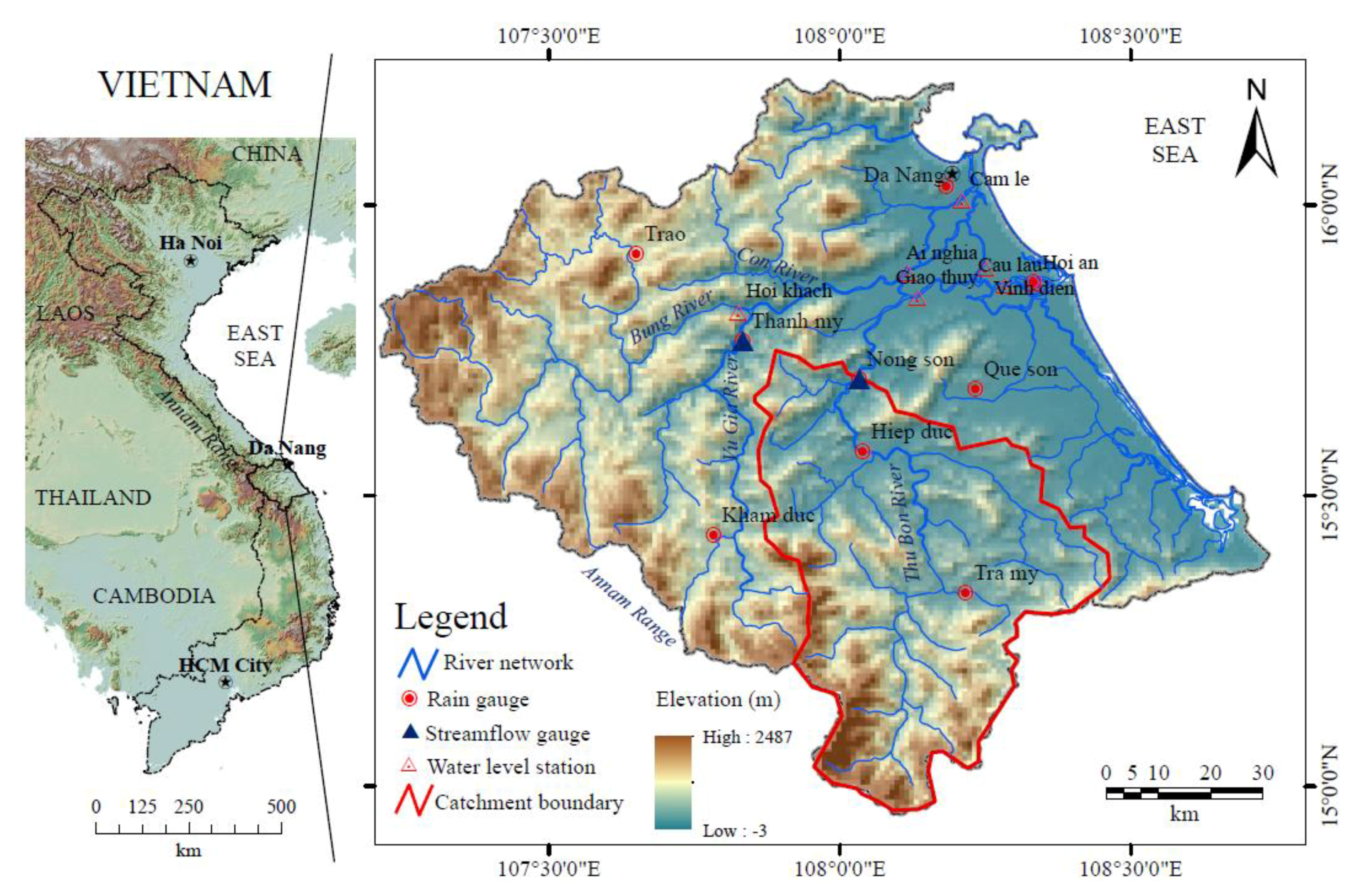
2.1. Description of the Study Area

The central region of Vietnam is characterized by a mountain range to the west and narrow flood plains along the coast line to the east. With respect to climate and weather patterns, the region is influenced by a tropical monsoon regime with two distinguish wet and dry seasons. The wet season (September–December), a period known as a transition phase from boreal summer to winter monsoon, is often affected by intense orographic rainfall that results from tropical depressions and storms. As a result, Central Vietnam is well-known as a flood-prone area of the country. With regard to flood hazard, statistics show that the floods seem to be getting more severe and frequent; it is found that six out of the seven major floods in the last 50 years occurred between 1995 and 2010. This indicates an increasing trend of flood risk in the region, even in the present day climate.

The Upper Thu Bon catchment selected in this study has a drainage area of 3150 km², as delineated at the Nong Son stream gauge (Figure 1). It is a tributary of Vu Gia-Thu Bon river system, the fifth largest river basin in the Central Vietnam and covering most parts of Quang Nam and Da Nang provinces. In terms of land use, the catchment is mainly characterized by natural forests; however, rapid changes of land use for agricultural production have accelerated runoff responses. In addition, favored by a steep terrain, many reservoirs were constructed, but most of them were designed for hydropower generation and with limited capacity for flood control. Thus, there is indeed a requirement of future flood information for updating reservoir operation rules to reduce flood threats in downstream areas of the river.

2.2. Hydro-Meteorological Data

Historical hydro-meteorological data is conventionally used for climate model bias correction, hydrological model calibration-validation, and also for representing the baseline climate condition. In the Vu Gia-Thu Bon river system, the ground observation network is quite scattered and most of the observation sites are recording hydro-meteorological variables on a daily time scale. Figure 1 illustrates observation sites. There are nine rain gauges. Two of them (Tra My and Da Nang) are classified as atmospheric stations measuring hourly rainfall and other variables such as temperature, evaporation, and humidity. The remaining sites merely record the rainfall on a daily basis. Two streamflow gauges (Nong Son and Thanh My) measure hourly discharge and water level; the other six observation sites only record the water level. These sites have been measuring rainfall and streamflow since late 1970s to present and the data can be accessed from Vietnam Meteorological Hydrological Administration.

2.3. CMIP5 High-Resolution Climate Model Experiments

As clearly described in the literature [30], the CMIP5 was built to provide a standard set of climate simulations for the Fifth Assessment Report of IPCC (IPCC-AR5) and critical inputs for further investigations of climate change and its impacts at local scales. The ensemble of hundreds of experiments provided by more than fifty models, from modelling groups around the world, was included in the CMIP5. Individual groups performed experiments of either the long-term or the near-term; the long-term spans from the mid-nineteenth century through the twenty-first century, meanwhile the nearer term is out to 2035. The near-term decadal prediction experiments are a distinguished feature to CMIP. They were initialized from observed states of the climate system to explore climate predictability and prediction on decadal to multi-decadal timescales. More importantly, the CMIP5 show remarkable improvements to those of the previous phase (CMIP3), for example: (i) the better treatment of atmospheric chemistry; (ii) the larger number of experiments; and (iii) especially the model spatial resolution. The average grid size of CMIP5 is about 100 km on a side. However, some modelling groups designed high-resolution models with the horizontal resolutions of the order of 20–60 km with attempts for further understanding the future climate change at local scales.

The present study utilizes the daily rainfall simulations derived from high-resolution multi-model experiments performed by three leading climate modelling institutions, including: (i) Meteorological Research Institute of Japan (MRI); (ii) Japan Agency for Marine-Earth Science and Technology, Atmosphere and Ocean Research Institute (The University of Tokyo), and National Institute for Environmental Studies (MIROC); and (iii) Geophysical Fluid Dynamics Laboratory of The United States of America (GFDL). The experiments are for two time periods, the baseline climate (1979–2008) and the near-term climate (2026–2035). The baseline climate experimented with the mean monthly sea surface temperature (SST) observed in the same period. Meanwhile, for future climate, MRI performed the experiment using SST data based on the projections by the multi-model ensembles according to the A1B emission scenario, MIROC and GFDL applied prescribed SST (the multi-model mean over the four representative concentration pathway scenarios) and sea ice concentration anomalies. Various model runs (MIROC and GFDL) and parameterization schemes (MRI) were experimented for these high-resolution climate models; whereas the decadal prediction experiments were initialized with observed recent ocean and sea ice conditions.

Table 1. Selected CMIP5 high-resolution climate models and experiments.

Name of Modelling Group	CMIP5 Official Model-Name	Spatial Resolution	Experiment *
Meteorological Research Institute of Japan	MRI-AGCM3.2S	20 km	r1i1p1 (Expt-1)
	MRI-AGCM3.2H	60 km	r1i1p1 (Expt-2) r1i1p2 (Expt-3) r1i1p3 (Expt-4)
Geophysical Fluid Dynamics Laboratory-USA	GFDL-HIRAM-C360	25 km	r1i1p1(Expt-5) r2i1p1 (Expt-6)
Japan Agency for Marine-Earth Science and Technology, Atmosphere and Ocean Research Institute (The University of Tokyo), and National Institute for Environmental Studies, Japan	MIROC-4H	60 km	r1i1p1 (Expt-7) r2i1p1 (Expt-8) r3i1p1 (Expt-9)

* r, i, and p denote experiment number, initialization, and parameterization scheme of a model experiment, respectively.

below presents selected CMIP5 high-resolution climate models and nine available experiments for this study.

2.4. Model Bias Correction

High resolution models exhibit the capability of simulating heavy rainfall at local scales [31]; however, they still tend to predict the tendencies of future climate states rather than making precise predictions of specific events that are likely to occur. For that reason, most impact studies applied model bias correction techniques to improve the model simulations (e.g. [32,33]). The decadal prediction experiments need special post processing of the model outputs [30].

Conventional bias correction techniques include simple scaling methods (e.g., [6,32,33]), complicated multiple regression-base models (e.g., [16,34]) and comprehensively reviewed in the literature [35]. Another work [6] of this research series presented a regression-based bias correction model to correct extreme rainfall simulated by a MRI super-high resolution model (Expt-1). The correction model considered the effect of orographic uplifts causing heavy rainfall during tropical storms in selection of predictor variables. As a result, in addition to the rainfall variable, the vertical pressure velocities at low pressure layers have been used to formulate empirical equations. This method showed a good reference for similar studies. However, other high-resolution CMIP5 models included in this study show inadequate details of wind field simulations. Thus, this study adopts a combined scaling and quantile mapping method [36] to correct the area average daily rainfall simulated by CMIP5 models and aimed to overcome overestimated or underestimated future extreme daily precipitation, in some cases produced by ordinary scaling methods [32].

In a short description, datasets of observed rainfall and that simulated by CMIP5 models are first ranked for the entire present day climate. Daily scaling factors are defined for extreme samples with non-exceedance probability greater than 99.5% and then used to correct the corresponding extreme rainfall values simulated by the models for future climate. The remaining ranked samples are then rearranged in time sequence and monthly scaling factors are calculated and applied to correct the daily rainfall simulated by the models as described in the literature [32].

2.5. Hydrological Simulation

For this study, the corrected area average rainfall in the previous step will be used to drive a calibrated super-tank model for streamflow simulations. The super-tank is a semi-distributed hydrological model that was specially developed for both continuous and event-base runoff simulations. The model concept is based on a hydrological process represented by linear cascade tanks [37]; however, it focuses on more physical-based features and takes advantages of spatial available datasets (e.g., digital elevation model, land use, and soil type). As a result, the model has successfully shown its robustness in flood forecasting and climate change impact assessment across a wide range of spatial and temporal scales, especially for catchments with limited data (e.g., [20,38,39]). The details of model structure can be found in the literature [39].

In the previous study [20], the super tank model was setup, calibrated and validated for the Upper Thu Bon River basin using daily datasets of rainfall and discharge measured in the baseline climate (1979–2008). Additional to meteorological datasets, model input data also included information on physical properties of the catchments such as land use, soil type and topographic features. All input data was spatially set for each model grid cell. Model simulation was set on a daily basis with three criteria including: Nash–Sutcliffe efficiency (NSE), standard deviation ratio (RSR), and percent bias (PBIAS) were used to evaluate the model performance. The period of 1989–2008, during which most of the extreme events occurred, was used for model calibration, and the rest of the dataset was used for model validation. It was found that the super-tank model demonstrated reasonable reproduction of the daily streamflow, especially during high flow periods for the Upper Thu Bon River basin. As classified in the literature [40] the super-tank model was evaluated with a “very good” performance in the daily streamflow simulation for the calibration dataset and “good” performance in the case of model validation. As a result, the model was suggested to be a suitable tool for flood studies on climate change impacts. Detailed model performance evaluation was addressed in the literature [20].

2.6. Flood Frequency Analysis

Flood frequency analysis is useful for flood risk management and design of flood control structures. The scales of most flood control structures were determined under the consideration of rainfall variability, but variation properties are stationary with time [41]. Frequency curves had been established based on variations of the rainfall recorded in the past; they are perhaps no longer valid under a changing climate. As it has been found that the most extreme events occurred in the last several decades were distributed beyond the margins of those observed in the history. This study again employed a method presented in the literature [1] and [14] for determining rainfall and flood extremes with chosen return periods (Tr) for the baseline and future climates. The method employs the Gumbel extreme value distribution fitting of the annual maximum discharge using the L-moments approach [42], as expressed in Equation (1). It was found that the selected extreme value distribution showed advantages over other distributions for the cases of relatively small data sample [1].

$$Q(Tr)=\xi -\alpha \ln (-\ln (1-\frac{1}{Tr}))$$

(1)

where α and ξ are the scale and location parameters of the analytical Gumbel distributions.

2.7. Design Hyetograph/Hydrograph

The rainfall extremes are commonly represented by duration-based indices, for instance, the highest rainfall amount in a certain period of time (yearly- or decadal-basis) is considered an extremely severe event that might threaten the life and devastate properties and the environment. In this study, the model bias-corrected rainfall exhibits advantages for the analyses of intensity-duration-frequency based on the annual maximum 1-, 3-, and 5-day rainfall and helps to construct some types of design hyetographs. Similar to the previous work of this research series [16], the present study also applies the Chicago method [43] to model the temporal distribution of the design hyetographs based on the intensity–duration–frequency curves derived from multi-model simulations for the baseline and near future climates. This approach considers the asymmetry of the design hyetographs, a common feature of cyclone rainstorms in West Pacific regions [44]. Detailed steps for parameter estimations (using a non-linear least squares method) can be found in the literature [16]. The multi-model simulations derived design hyetographs of different return periods are subsequently used to drive the super tank model to simulate corresponding design hydrographs.

2.8. Estimate of Confidence Interval

As previously addressed, climate model structure and parameterization scheme dominate uncertainties in rainfall estimation. Different model experiments obviously provide different simulations of the climate state even under the same model initial and boundary conditions. This study adopts a simple approach addressed in the literature [45] to estimate the confident interval of the projections. In a general form, it is assumed that changes in streamflow are normal distribution, then the 95% confidence interval ($\Delta$) of the changes is defined as a function of the change estimated by the multi-model ensemble mean ($\overline{\Delta Q}$) and standard deviation (${\delta }_{\Delta Q}$), as expressed in Equations (2) and (3). Note that this principle is also considered to apply for such other variables as the rainfall extremes.

$$\Delta =\overline{\Delta Q}\pm 2{\delta }_{\Delta Q}$$

(2)

$${\delta }_{\Delta Q}={\left[\frac{1}{N}{\displaystyle \sum _{i=1}^N{(\Delta Qi-\overline{\Delta Q})}^2}\right]}^{1/2}$$

(3)

where N is the total number of model simulations; $\Delta Q_i$ denotes the model simulated streamflow change.

3. Results and Discussion

Before addressing the investigation of flood extremes in the future, it is notable that the CMIP5 near-term experiments are on decadal timescales so that the selected 30-year time-slice representing the baseline climate is divided into three decadal time-slices: 1979–1988, 1989–1998, and 1999–2008. Thus, the rainfall and flood extremes will be analyzed for individual decadal time-slices then averaged to represent the baseline climate (1979–2008). In addition, similar to other approaches (e.g., [1,2,3,13]), the simulation of streamflow excludes the influences of flood control structures (e.g. reservoirs and upcoming river improvement works) and non-climatic factor such as changes in land use. Hence, this assessment attempts to explore potential changes in the flood extremes. Another remark included in the present study is that increasing surface temperature is likely to enhance evapotranspiration processes. However, the present study focuses on the flood extremes, so the effect of evapotranspiration variability on the flood runoff is omitted.

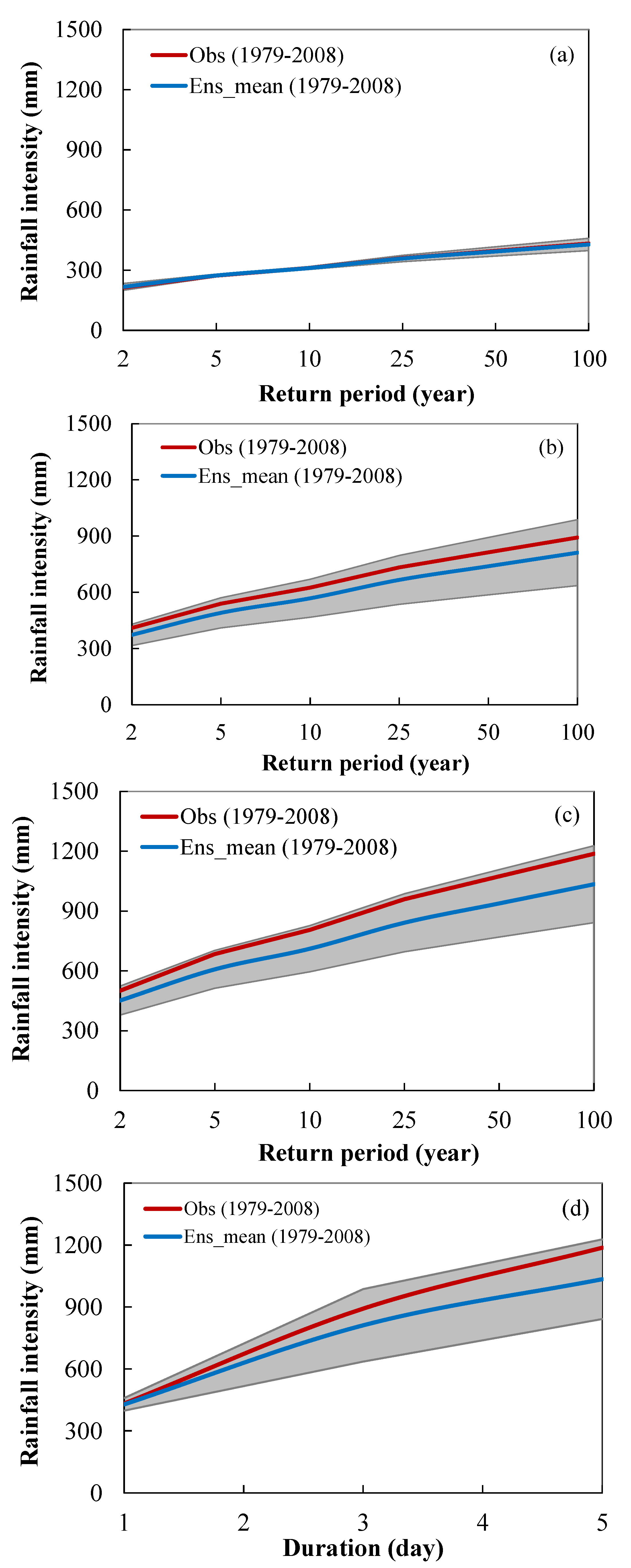
3.1. Corrected Rainfall

In this study, the inverse distance weighting interpolation method is applied for estimating area-average daily rainfall from grid-based (climate model outputs) and point observation rainfall data. Figure 2 exhibits the comparison of the rainfall derived from direct model outputs and model bias correction against the observation. It is clear that the direct high-resolution CMIP5 model outputs underestimate the extreme rainfall; however, it is found that the applied bias correction techniques have significantly improved the estimates of the extreme rainfall. The quantile mapping shows the best fit of the multi-model ensemble mean to the perfect line (Figure 2a); the spread of model variation is insignificant. With respect to temporal correction, the corrected mean monthly rainfall demonstrates a good agreement with the observation, except slight underestimates in the wettest months (October and November) of the year (Figure 2b).

Figure 3 illustrates a comparison of historical depth and frequency for rainstorm durations from 1- to 5-day between the observation and corrected multi-model simulations. Results show that the maximal 1-day rainfall intensity of various return periods is well reproduced for the baseline climate (Figure 3a). But discrepancies are observed for the greater rainstorm durations (Figure 3b–d). These can be understood as the applied correction techniques, but still maintain the temporal structure of the multi-model simulations. It is interesting to see that the upper limit of the 95% confident interval seems to have a good agreement with the observation.

Similar model bias correction and frequency analyses are then applied for the near future climate simulations. In this study, the pattern of changes in rainfall and flood extremes is explored merely based on simulated datasets in the past and future. Figure 4 shows changes in depth–duration–frequency derived from multi-model simulations for the baseline and near future climates. Increased rainfall intensity is found larger for greater return periods and also associated with a larger spread of model variation (Figure 4a–c). It is apparent that there is a slight variation in the extreme events that occurs with a frequency of every two years. However, those extreme events, with fifty years return period, (Tr = 50-year) in the future is very likely to exceed the event with the return period of one hundred years (Tr = 100-year) in the baseline climate (Figure 4d).

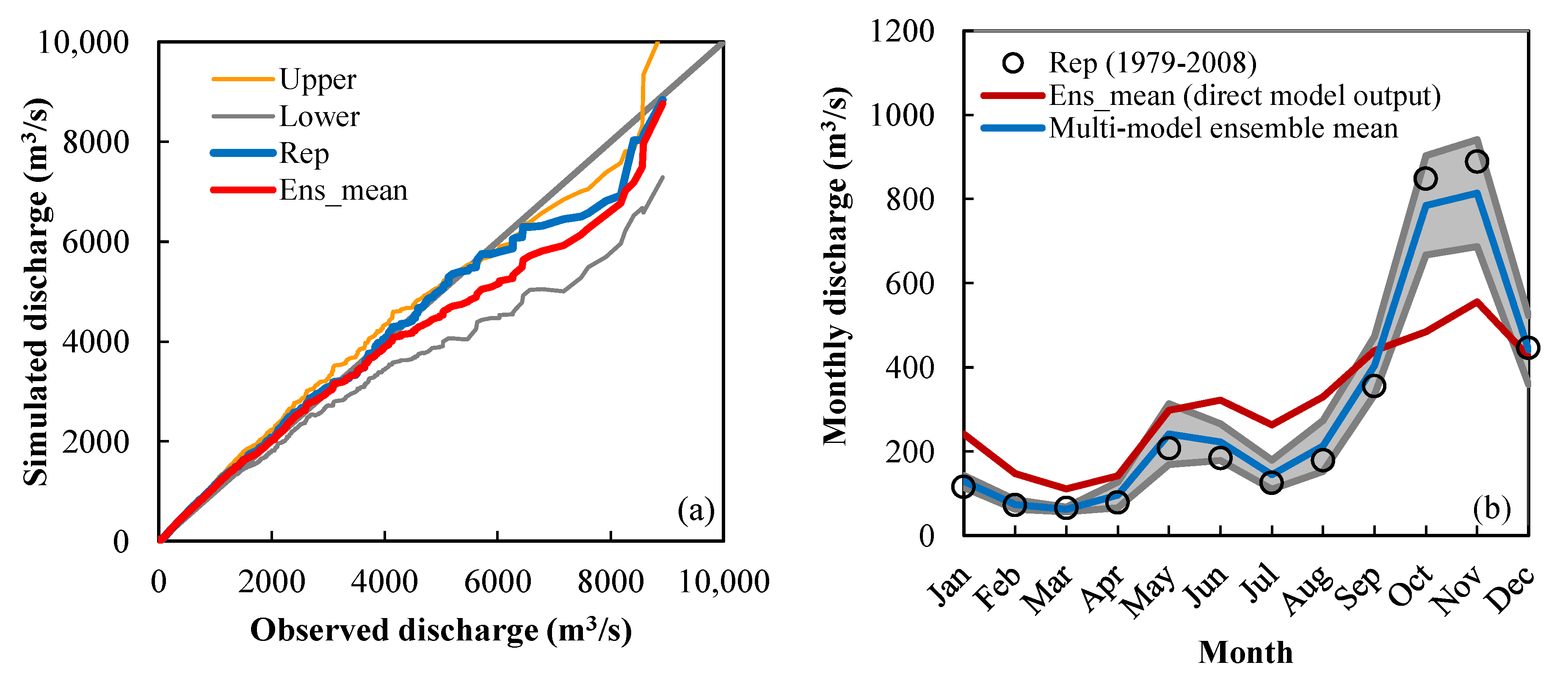
3.2. Simulated Discharge

The corrected daily rainfall from multi-model experiments is used to drive the calibrated super tank model for streamflow simulations. Figure 5a,b show the quantile mapping of daily discharge and comparison of the mean monthly streamflow for the baseline climate, respectively. It is found that simulated discharge using the corrected rainfall also exhibits a reasonable agreement with that reproduced (Rep) using the observed rainfall. Similar to the discrepancies identified for the corrected rainfall, the simulated streamflow is underestimated during the wettest period of the year.

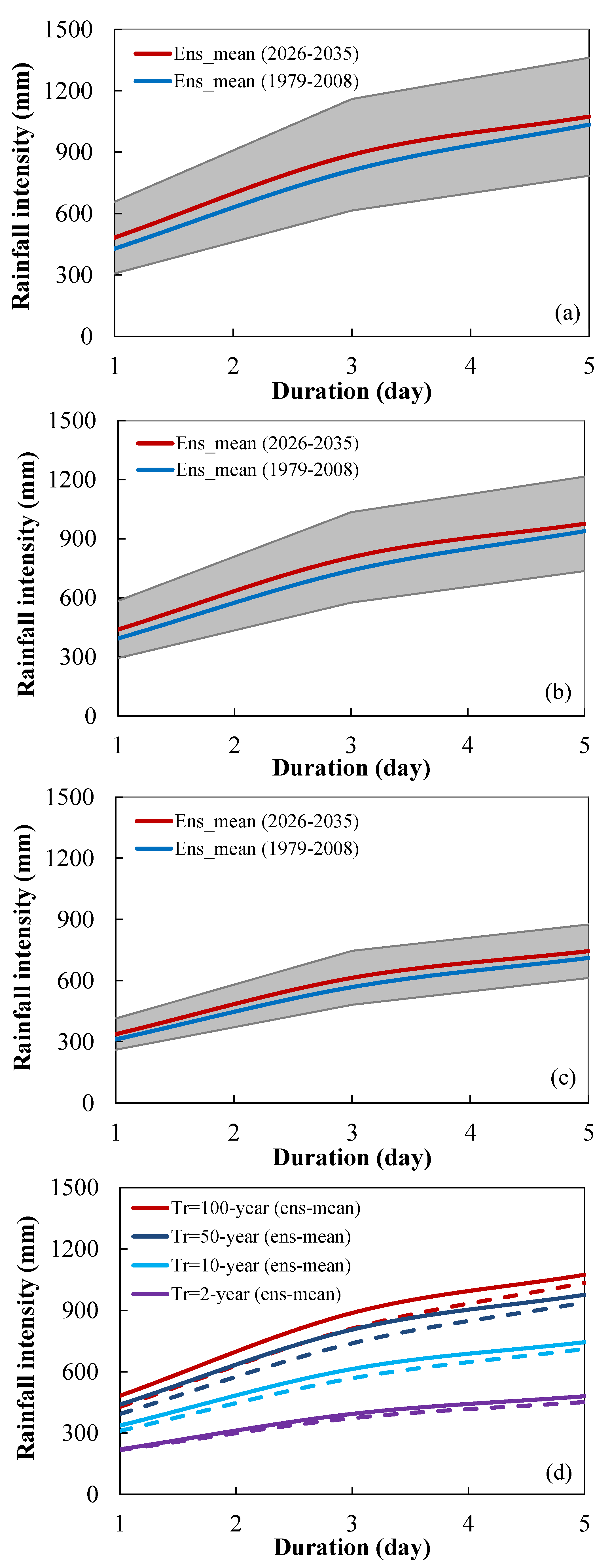
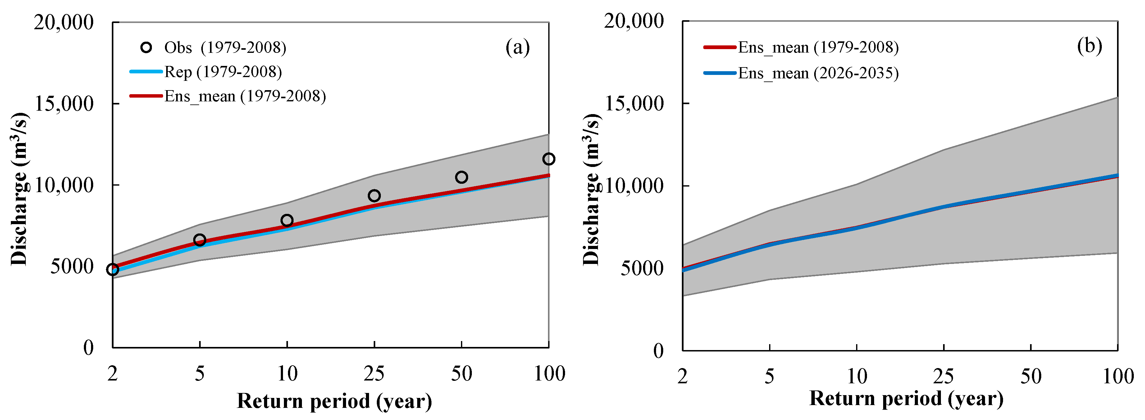
3.3. Change in Flood Extremes

With regard to flood extremes, they are defined as those which have caused losses of life and excessive damage to property. In the Vu Gia-Thu Bon river system, bank-full discharge usually triggered serious damages in lowland areas. The peak discharge corresponding to the 2-year return period is commonly considered representative of river bank-full conditions [46]. Figure 6a shows the comparison of the flood extremes of different frequencies derived from streamflow simulations using the observed rainfall (Rep) and corrected rainfall (multi-model ensemble mean) for the baseline climate. Though the discrepancies are previously addressed for the simulated discharge, it is found, a good agreement between the reproduced and simulated flood extremes. In this case, both of them show slightly lower magnitudes as compared to actual observation. The pattern of change in flood extremes in the future climate is illustrated in Figure 6b. The result indicates similar magnitudes of the flood extremes in the future to the baseline period based on the near-term experiments by high-resolution climate models. However, the spread among model experiments seems to be larger along with greater return periods. The flood extremes (not shown) derived from the experiments (Expt-1 to Expt-4) performed by MRI indicating significant variations in model projections, because MRI attempted to examine the influence of different model resolutions and parameterization schemes. Expt-1 and Expt-2 employed a new cumulus convection scheme which is considerably improved the climatology of tropical convection (“Yoshimura Scheme”, [47]) project the flood extremes near the upper limit of the confident interval and those selected conventional convection schemes “Arakawa–Schubert Scheme [48]” (Expt-3) and “Kain–Fritsch Scheme [49]” (Expt-4) project the flood extremes toward the lower limit of the confident interval. The super high- resolution model experiment (Expt-1) projects the largest flood extremes. While the remaining experiments (Expt-5 to Expt-9) offer a slight spread in model projections as they were designed merely for examining the changes in the projections corresponding to various model runs.

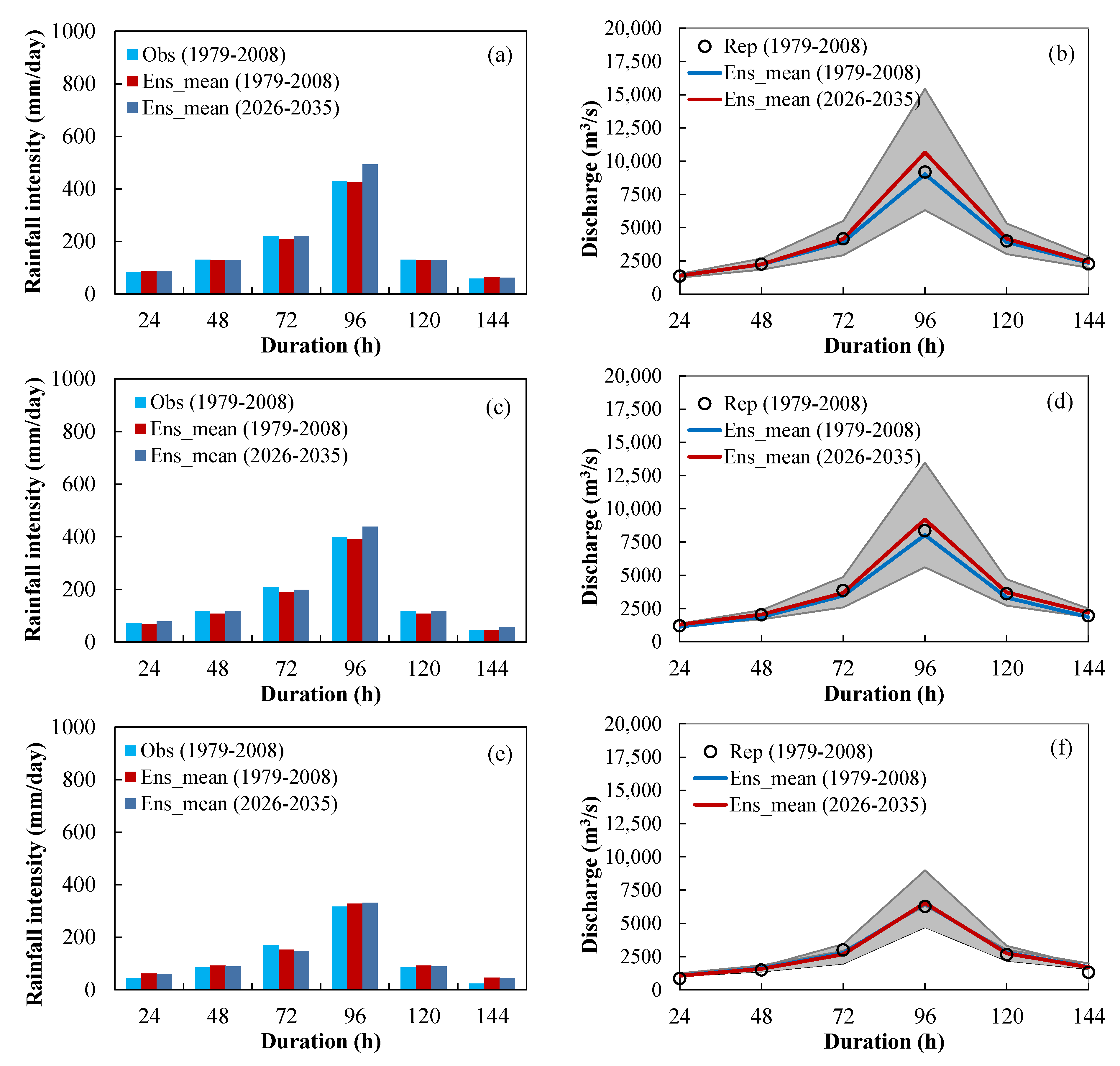
3.4. Design Storm Hydrographs

The flood extremes in the selected catchment are then further evaluated through the construction of design storm hyetographs/hydrographs which are considered essential for determining the scales of water-related systems, especially the flood control structures. The design storm hyetographs are constructed using intensity–duration–frequency (the inverse of depth–duration–frequency) curves previously established. Figure 7 illustrates examples of design storm hyetographs/hydrographs corresponding to typical return periods of 100-year, 50-year, and 10-year.

The design storm hyetographs (Figure 7a,c,e) for the baseline climate are derived from the observed and multi-model bias corrected rainfall. The results show similar rainfall intensities for both cases. Again, these indicate reasonable model bias correction used in this study. For future climate, the projected hyetographs are apparently comparable to those in the baseline climate, except increases in the peaks. As a result, the design hydrographs reflect the same pattern of changes in the peak discharge as seen in Figure 7b,d,f. The increases are found significant for more extreme events. The peak of 100-year and 50-year return period floods tend to increase about 18% and 15%, respectively. Especially, the peak of 50-year return period flood in the future tends to exceed those corresponding to 100-year return period in the baseline climate. Meanwhile, there is very likely no change in the peak of low return period floods (e.g., 10-year and 2-year). It is also noted that uncertainties in the projections are quantified larger for more extreme events.

4. Conclusions

An assessment of flood extremes in the future is performed in this study, the extension of the previous work on exploring rainfall-runoff responses of small scale catchments under the influence of a changing climate [20]. The assessment is tested for the Upper Thu Bon river basin, a flood prone area in Vietnam, using the downscaled CMIP5 high-resolution ensemble projections of near-term climate. The applied model bias correction techniques show reasonable performance with regard to improved rainfall simulations by the climate models. The corrected rainfall is useful for flood extreme analyses. Two methods, Gumbel extreme value distribution fitting of the annual maximum discharge and construction of design hydrograph, are implemented in this study. The former method indicates almost no changes in the flood extremes in the future compared to the baseline climate. However, the later method indicates increases (approximately 20%) in the peaks of very extreme events in the future climate, especially, the flood peak of 50-year return period tends to exceed the flood peak of 100-yr return period in the baseline climate. Meanwhile, the peaks of shorter return period floods are projected with a very slight change. As a result, this exploration is believed to be critical to making informed decisions for implementing flood control and risk reduction in this river basin and the downstream areas as well.

It is the nature of any climate change impact study that there exist uncertainties in the projection results. Results indicate that the spread among model experiments is projected larger for greater return period events. Model physical parameterization schemes and spatial resolution seem to cause considerable uncertainties. Experiments based on the improved tropical convection scheme seems to project large increases in flood extremes; while different model runs show less sensitivity to the future projections.

References

1. Hirabayashi, Y.; Mahendran, R.; Koirala, S.; Konoshima, L.; Yamazaki, D.; Watanabe, S.; Kim, H.; Kanae, S. Global flood risk under climate change. Nat. Clim. Chang. 2013, 3, 816–821. [Google Scholar] [CrossRef]
2. Wilby, R.L.; Beven, K.J.; Reynard, N.S. Climate change and fluvial flood risk in the UK: More or the same. Hydrol. Process. 2008, 22, 2511–2523. [Google Scholar] [CrossRef]
3. Milly, P.C.D.; Wetherald, R.T.; Dunne, K.A.; Delworth, T.L. Increasing risk of great floods in a changing climate. Nature 2002, 415, 514–517. [Google Scholar] [CrossRef]
4. Ulbrich, U.; Brucher, T.; Fink, A.H.; Leckebusch, G.C.; Kruger, A.; Pinto, J.G. The central European floods of August 2002: Part 1—Rainfall periods and flood development. Weather 2003, 58, 371–377. [Google Scholar] [CrossRef]
5. Fowler, A.M.; Hennessy, K.J. Potential impacts of global warming on the frequency and magnitude of heavy precipitation. Nat. Hazards 1995, 11, 283–303. [Google Scholar] [CrossRef]
6. Prudhomme, C.; Reynard, N.; Crooks, S. Downscaling of global climate models for flood frequency analysis: Where are we now? Hydrol. Process. 2002, 16, 1137–1150. [Google Scholar] [CrossRef]
7. Ekstro¨m, M.; Fowler, H.J.; Kilsby, C.G.; Jones, P.D. New estimates of future changes in extreme rainfall across the UK using regional climate model integrations. 2. Future estimates and use in impact studies. J. Hydrol. 2005, 300, 212–233. [Google Scholar] [CrossRef]
8. Kay, A.L.; Jones, R.G.; Reynard, N.S. RCM rainfall for UK flood frequency estimation. II. Climate change results. J. Hydrol. 2006, 318, 163–172. [Google Scholar] [CrossRef]
9. IPCC (Intergovernmental Panel on Climate Change). Climate Change 2007: The Physical Science Basis; Cambridge University Press: Cambridge, UK; New York, NY, USA, 2007. [Google Scholar]
10. IPCC (Intergovernmental Panel on Climate Change). Climate Change 2013: The Physical Science Basis; Cambridge University Press: Cambridge, UK; New York, NY, USA, 2013. [Google Scholar]
11. Kharin, V.V.; Zwiers, F.W.; Zhang, X.; Hegerl, G.C. Changes in temperature and rainfall extremes in the IPCC ensemble of global coupled model simulations. J. Clim. 2007, 20, 1419–1444. [Google Scholar] [CrossRef]
12. Vidal, J.P.; Wade, S.D. Multimodel projections of catchment-scale precipitation regime. J. Hydrol. 2008, 353, 143–158. [Google Scholar] [CrossRef]
13. Koirala, S.; Hirabayashi, Y.; Mahendran, R.; Kanae, S. Global assessment of agreement among streamflow projections using CMIP5 model outputs. Environ. Res. Lett. 2014. [Google Scholar] [CrossRef]
14. Alfieri, L.; Burek, P.; Feyen, L.; Forzieri, G. Global warming increases the frequency of river floods in Europe. Hydrol. Earth Syst. Sci. 2015, 19, 2247–2260. [Google Scholar] [CrossRef] [Green Version]
15. Dankers, R.; Feyen, L. Climate change impact on flood hazard in Europe: An assessment based on high-resolution climate simulations. J. Geophys. Res. 2008, 113, D19105. [Google Scholar] [CrossRef]
16. Nam, D.H.; Udo, K.; Mano, A. Assessment of future flood intensification in Central Vietnam using a super-high-resolution climate model output. J. Water Clim. Chang. 2013, 4, 373–389. [Google Scholar] [CrossRef]
17. Kitoh, A.; Ose, T.; Kurihara, K.; Kusunoki, S.; Sugi, M. Projection of changes in future weather extremes using super-high-resolution global and regional atmospheric models in the KAKUSHIN program: Results of preliminary experiments. Hydrol. Res. Lett. 2009, 3, 49–53. [Google Scholar] [CrossRef]
18. Toan, D.D.; Tachikawa, Y.; Shiiba, M.; Yorozu, K. River discharge projection in Indochina Peninsula under a changing climate using the MRI-AGCM3.2S dataset. Ann. J. Hydraul. Eng. 2013, 69, 37–42. [Google Scholar]
19. Prudhomme, C.; Jakob, D.; Svensson, C. Uncertainty and climate change impact on the flood regime of small UK catchments. J. Hydrol. 2003, 277, 1–23. [Google Scholar] [CrossRef]
20. Nam, D.H.; Duong, P.C.; Thuan, D.H.; Mai, D.T.; Dung, N.Q. Near-term runoff response at a river basin scale in Central Vietnam assessed using direct CMIP5 high-resolution model outputs. Water 2018, 10, 477. [Google Scholar] [CrossRef]
21. Kay, A.L.; Davies, H.N.; Bell, V.A.; Jones, R.G. Comparison of uncertainty sources for climate change impacts: Flood frequency in England. Clim. Chang. 2009, 92, 41–63. [Google Scholar] [CrossRef]
22. Fowler, H.J.; Blenkinsop, S.; Tebaldi, C. Linking climate change modelling to impacts studies: Recent advances in downscaling techniques for hydrological modelling. Int. J. Climatol. 2007, 27, 1547–1578. [Google Scholar] [CrossRef]
23. Allan, R.P.; Soden, B.J. Atmospheric warming and the amplification of precipitation extremes. Science 2008, 321, 1481–1484. [Google Scholar] [CrossRef] [PubMed]
24. Palmer, T.N.; Raisanen, J. Quantifying the risk of extreme seasonal precipitation events in a changing climate. Nature 2002, 415, 512–514. [Google Scholar] [CrossRef]
25. Scher, S.; Haarsma, R.J.; de Vries, H.; Drijfhout, S.S.; van Delden, A.J. Resolution dependence of extreme precipitation and deep convection over the Gulf Stream. J. Adv. Model. Earth Syst. 2017, 9, 1186–1194. [Google Scholar] [CrossRef] [Green Version]
26. Oouchi, K.; Yoshimura, J.; Yoshimura, H.; Mizuta, R.; Kusunoki, S.; Noda, A. Tropical cyclone climatology in a global-warming climate as simulated in a 20 km-mesh global atmospheric model: Frequency and wind intensity analysis. J. Meteorol. Soc. Jpn. 2006, 84, 259–276. [Google Scholar] [CrossRef]
27. Wehner, M.F.; Smith, R.L.; Bala, G.; Duffy, P. The effect of horizontal resolution on simulation of very extreme us precipitation events in a global atmosphere model. Clim. Dynam. 2010, 34, 241–247. [Google Scholar] [CrossRef]
28. Ngai, S.T.; Tangang, F.; Juneng, L. Bias correction of global and regional simulated daily precipitation and surface mean temperature over Southeast Asia using quantile mapping method. Glob. Planet. Chang. 2017, 149, 79–90. [Google Scholar] [CrossRef]
29. Meaurio, M.; Zabaleta, A.; Boithias, L.; Epelde, A.M.; Sauvage, S.; Sanchez-Perez, J.M.; Srinivasan, R.; Antiguedad, I. Assessing the hydrological response from an ensemble of CMIP5 climate projections in the transition zone of the Atlantic region (Bay of Biscay). J. Hydrol. 2017, 548, 46–62. [Google Scholar] [CrossRef]
30. Taylor, K.E.; Stouffer, R.J.; Meehl, G.A. An overview of CMIP5 and the experiment design. Bull. Am. Meteorol. Soc. 2012, 93, 485–498. [Google Scholar] [CrossRef]
31. Endo, H.; Kitoh, A.; Ose, T.; Mizuta, R.; Kusunoki, S. Future changes and uncertainties in Asian precipitation simulated by multiphysics and multi-sea surface temperature ensemble experiments with high resolution Meteorological Research Institute atmospheric general circulation models (MRI-AGCMs). J. Geophys. Res. 2012, 117. [Google Scholar] [CrossRef]
32. Kiem, A.S.; Ishidaira, H.; Hapuarachchi, H.P.; Zhou, M.C.; Hirabayashi, Y.; Takeuchi, K. Future hydroclimatology of the Mekong River basin simulated using the high-resolution Japan Meteorological Agency (JMA) AGCM. Hydrol. Process. 2008, 22, 1382–1394. [Google Scholar] [CrossRef]
33. Takara, K.; Kim, S.; Tachikawa, Y.; Nakakita, E. Assessing climate change impact on water resources in the Tone river basin, Japan, using super-high resolution atmospheric model output. J. Disaster Res. 2009, 4, 12–22. [Google Scholar] [CrossRef]
34. Hay, L.E.; Clark, M.P. Use of statistically and dynamically downscaled atmospheric model output for hydrologic simulations in three mountainous basins in the western United States. J. Hydrol. 2003, 282, 56–75. [Google Scholar] [CrossRef]
35. Themeßl, M.J.; Gobiet, A.; Leuprecht, A. Empirical-statistical downscaling and error correction of daily precipitation from regional climate models. Int. J. Climatol. 2011, 31, 1530–1544. [Google Scholar] [CrossRef]
36. Inomata, H.; Takeuchi, K.; Fukami, K. Development of a statistical bias correction method for daily precipitation data of GCM20. Annu. J. Hydraul. Eng. 2011, 67, 247–252. [Google Scholar] [CrossRef]
37. Sugawara, M. The flood forecasting by a series storage type model. In Proceedings of the International Symposium on Flood and Their Computation, Leningrad, Russia, 15–22 August 1967; pp. 555–560. [Google Scholar]
38. Kato, H.; Mano, A. Flood runoff model on one kilometer mesh for the Upper Chang Jiang River. Proc. GIS RS Hydrol. Water Resour. Environ. 2003, 1, 1–8. [Google Scholar]
39. Nam, D.H.; Mai, D.T.; Udo, K.; Mano, A. Short-term flood inundation prediction using hydrologic-hydraulic models forced with downscaled rainfall from global NWP. Hydrol. Process. 2014, 28, 5844–5859. [Google Scholar] [CrossRef]
40. Moriasi, D.N.; Arnold, J.G.; van Liew, M.W.; Bingner, R.L.; Harmel, R.D.; Veith, T.L. Model evaluation guidelines for systematic quantification of accuracy in watershed simulations. Trans. ASABE 2007, 50, 885–900. [Google Scholar] [CrossRef]
41. Klein-Tank, A.M.G.; Zwiers, F.W.; Zhang, X. Analysis of extremes in a changing climate in support of informed decisions for adaptation. World Meteorol. Organ. 2009, 72, 1–52. [Google Scholar]
42. Hosking, J.R.M. L-Moments: Analysis and estimation of distributions using linear combinations of order statistics. J. R. Stat. Soc. B Method. 1990, 52, 105–124. [Google Scholar] [CrossRef]
43. Keifer, C.J.; Chu, H.H. Synthetic storm pattern for drainage design. J. Hydraul. Div. 1957, 83, 1–25. [Google Scholar]
44. Cheng, K.S.; Hueter, I.; Hsu, E.C.; Yeh, H.C. A scale invariant Gauss-Markov model for design storm hyetographs. J. Am. Water Resour. Assoc. 2001, 37, 723–735. [Google Scholar] [CrossRef]
45. Giorgi, F.; Mearns, L.O. Calculation of average, uncertainty range, and reliability of regional climate changes from AOGCM simulations via the “reliability ensemble averaging” (REA) method. J. Clim. 2002, 15, 1141–1158. [Google Scholar] [CrossRef]
46. Carpenter, T.M.; Sperfslage, J.A.; Georgakakos, K.P.; Sweeney, T.; Fread, D.L. National threshold runoff estimation utilizing GIS in support of operational flash flood warning systems. J. Hydrol. 1999, 224, 21–44. [Google Scholar] [CrossRef]
47. Yukimoto, S.; Yoshimura, H.; Hosaka, M.; Sakami, T.; Tsujino, H.; Hirabara, M.; Tanaka, T.Y.; Deushi, M.; Obata, A.; Nakano, H.; et al. Meteorological Research Institute-Earth System Model v1 (MRIESM1)—Model Description; Technical Reports; Meteorological Research Institute: Tsukuba, Japan, 2011. Available online: http://www.mri-jma.go.jp/Publish/Technical/DATA/VOL_64/tec_rep_mri_64.pdf (accessed on 31 March 2011).
48. Arakawa, A.; Schubert, W.H. Interaction of acumulus cloud ensemble with the large-scale environment. PartI. J. Atmos. Sci. 1974, 31, 674–701. [Google Scholar] [CrossRef]
49. Kain, J.S.; Fritsch, J.M. Convective parameterization for mesoscale models: The Kain-Fritsch scheme. The representation of cumulus convection in numerical models. Meteorol. Monogr. 1993, 46, 165–170. [Google Scholar]
Figure 1. Map of the Upper Thu Bon river basin as delineated at Nong Son stream gauge and locations of the hydro-meteorological observation [20].
Water 11 00634 g001
Figure 2. Comparison of the area average rainfall between direct model output and model bias correction in the baseline climate (1979–2008): (a) daily precipitation quantiles; and (b) mean monthly rainfall.
Water 11 00634 g002
Figure 3. Comparison of historical depth and frequency for rainstorm durations of 1-day (a), 3-day (b), 5-day (c), and depth duration with 100-year return period (d) between observed rainfall and model bias correction (shaded areas show 95% confidence intervals for multi-model simulations).
Water 11 00634 g003
Figure 4. Comparison of depth duration frequency (ensemble mean) between the baseline climate (1979–2008) and near future climate (2026–2035) with 100-year (a), 50-year (b), 10-year (c) return periods with shaded areas showing 95% confidence intervals of the projected rainfall, and ensemble means of various frequencies (d) with solid and dashed lines representing the near future and baseline climates, respectively.
Water 11 00634 g004
Figure 5. Comparison of discharge simulated using the observed (Rep) and corrected rainfall (Ens_mean, upper and lower limits of 95% confidence intervals) against the reproduced discharge in the baseline climate (1979–2008): (a) daily discharge quantiles; and (b) mean monthly streamflow.
Water 11 00634 g005
Figure 6. (a) Verification of flood extremes reproduced (Rep) using the observed rainfall model bias correction (Ens_mean) against the observation (Obs); (b) Comparison of multi-model simulations for the baseline and near future climate with shaded areas showing 95% confidence intervals of the projected flood extremes.
Water 11 00634 g006
Figure 7. Design storm hyetographs and hydrographs for the Upper Thu Bon river basin constructed for the baseline and future climates with 100-year (a,b), 50-year (c,d), and 10-year (e,f) return periods and shaded areas shows 95% confidence intervals of the projected hydrographs.
Water 11 00634 g007