Seasonal, Annual, and Decadal Distribution of Three Rorqual Whale Species Relative to Dynamic Ocean Conditions Off Oregon, USA

1 Introduction

The blue economy is a booming sector offering the prospects of economic growth combined with a sustainable use of marine resources (Jouffray et al., 2020). However, as commercial interest and industrial development in the oceans increase, ecosystems are confronted with the cumulative impacts of human activities at an unprecedented pace (Golden et al., 2017). Since the 1970s, trends in global maritime traffic have risen (McCauley et al., 2015) and technological advances are enabling emergent uses of marine resources through the construction of marine renewable energy facilities and prospective seabed mining projects (Levin et al., 2020). The fishing industry has also grown rapidly since the 1960s to meet the expanding demand for seafood (Watson et al., 2015). If this ocean industrialization is not balanced with ecosystem conservation, habitat degradation and defaunation are expected to rapidly intensify at global and local scales (McCauley et al., 2015).

Dynamic spatial management can be an effective approach to avoid these resource conflicts between human activities and marine wildlife (Hyrenbach et al., 2000; Maxwell et al., 2015; Dunn et al., 2016; Hazen et al., 2018; Hausner et al., 2021). Yet, its success relies on knowledge of species distribution at appropriately resolved spatio-temporal scales. Species Distribution Models (SDMs) have become an indispensable tool to assess distributions of species in response to ocean dynamics (Gilles et al., 2016; Hazen et al., 2018; Abrahms et al., 2019) or in the context of climate change (Hazen et al., 2013; Becker et al., 2018; Derville et al., 2019), and thus can estimate vulnerability of species to human activities over vast regions (Mannocci et al., 2017; Virgili et al., 2018). These statistical correlative approaches fit empirical observations of species occurrence or abundance to environmental conditions to describe species ecological relationships and predict distributions over multiple spatial and temporal scales (Austin, 2007; Elith and Leathwick, 2009). Considerable research has been dedicated in recent years to improve the predictive performance of SDMs within a conservation perspective (Elith and Leathwick, 2009; Guisan et al., 2013; Yates et al., 2018).

Whale populations were decimated by decades of exploitation, resulting in the decline of important ecosystem functions (Savoca et al., 2021). Today, recovering populations face the consequences of the ocean’s growing anthropization, as whales are threatened by noise disturbance (Rolland et al., 2012; Pirotta et al., 2018), pollution (Zantis et al., 2021), climate change (Albouy et al., 2020), ship strikes (Redfern et al., 2013; Abrahms et al., 2019; Calambokidis et al., 2019; Schoeman et al., 2020) and entanglements (Knowlton et al., 2012; Saez et al., 2020). Due to their long life span and low reproductive rates, large whale populations are particularly slow to recover after direct or indirect impacts by human activities (Keen et al., 2021). To reduce exposure to the numerous threats whales face, spatially and temporally explicit regulations on human activities can be informed through SDMs generated at appropriate scales, with higher resolution predictions allowing more refined conservation measures.

In the California Current System (CCS) along the US West Coast, ocean industrializing is escalating and impacting whales (Carretta et al., 2021). Considerable research effort has been dedicated to monitoring whale population trends and understanding their distribution to reduce conflicts with increasing human activities in the CCS. Large-scale standardized shipboard surveys conducted in this region for three decades (e.g., Barlow et al., 2009; Becker et al., 2012; Forney et al., 2012; Becker et al., 2016; Becker et al., 2019, 2020b) and satellite tracking (e.g., Bailey et al., 2009; Hazen et al., 2017; Scales et al., 2017a; Abrahms et al., 2019; Palacios et al., 2019) have generated insight into the spatio-temporal patterns of habitat use of whales in the CCS. Among the species of concern are the rorqual whales such as humpback whales (Megaptera novaeangliae), blue whales (Balaenoptera musculus musculus), and fin whales (Balaenoptera physallus) that migrate along the US West Coast and seasonally forage on prey that is supported by high biological productivity generated by the eastern boundary current forming the CCS in summer and fall (Bograd et al., 2009). Following the “spring transition”, prevailing northwesterly winds drive surface waters offshore, which draws colder, nutrient-rich waters up from below and creates an intense upwelling system (Huyer, 1983). Rorqual whale feeding groups of blue, fin, and humpback whales found in the California/Oregon region of the CCS have been attributed to Distinct Population Segments (DPS) and stocks with different conservation status under the US Endangered Species Act. Humpback whales off California and Oregon belong to the threatened Mexican DPS and the endangered Central American DPS, while blue and fin whales are considered part of the Eastern North Pacific stock and the California/Oregon/Washington stock respectively (Carretta et al., 2021).

Recent studies indicated that habitat use patterns of these whales may change in response to variations in environmental conditions and prey availability in the CCS (Fossette et al., 2017; Irvine et al., 2019; Rockwood et al., 2020). Moreover, seasonally and annually changing conditions result in high temporal variability of whale distribution patterns (Becker et al., 2017; Becker et al., 2020b) leading to fluctuating exposure to human activities (Abrahms et al., 2019; Redfern et al., 2020; Santora et al., 2020). To accurately predict dynamics of whale distribution in specific regions of the CCS that is needed for effective management at appropriate scales, distribution models should be trained with fine-scale, current and locally acquired occurrence data. Yet, the majority of foundational whale species distribution modelling efforts in the CCS region were generated with movement data mostly acquired from satellite tags deployed on whales in California (Bailey et al., 2009; Hazen et al., 2017; Scales et al., 2017b; Abrahms et al., 2019; Palacios et al., 2019), or with density data acquired during broad shipboard surveys covering the entire US West Coast waters in summer-fall with transects spaced by 150 to 230 km (Barlow et al., 2009; Forney et al., 2012; Becker et al., 2020b). Comparatively less effort has been dedicated to winter-spring months, and to the more northern CCS waters on the continental shelf and slope off Oregon, where rapidly expanding human activities are also a cause of concern for whale populations, including marine renewable energies (BOEM, 2021a; BOEM, 2021b), navy training (US Department of the Navy, 2020), fishing (Feist et al., 2021) and ship traffic (Silber et al., 2020). Cetacean surveys conducted in Oregon with the purpose of deriving density estimates comprise year-round Minerals Management Survey transects (1989-1992, Brueggeman, 1992; Green et al., 1992), broad scale NOAA Southwest Fisheries Science Center summer-fall surveys (n = 7 years, 1996-2018, Barlow, 2016; Henry et al., 2020), one fine-scale summer survey on the shelf in 2000 (Tynan et al., 2005), and a year-round Pacific Continental Shelf Environmental Assessment (2011-2012; PaCSEA; Adams et al., 2014; Adams et al., 2016). Considering the spatio-temporal extent of these previous efforts, there is a relative paucity of recent and fine-scale whale distribution data in Oregon, particularly in nearshore waters during fall, winter and spring months that are a place and time of higher whale entanglement risk from fixed fishing gear (Feist et al., 2021). Therefore, as local whale populations recover from past exploitation (Carretta et al., 2021) and shift distributions in response to climate change (Becker et al., 2018), there is a need for a more modern, shelf-focused and finer-scale assessment of rorqual whale habitat use to predict exposure to human activities in Oregon.

In this study, we apply state-of-the-art SDM methods to fill a knowledge gap about the dynamic drivers of rorqual spatial distribution off Oregon. Whale densities are modeled from multi-platform surveys and assessed in relation to surface and subsurface oceanographic conditions and seabed topography. Given the shared ecological and biological traits, as well as similar conservation status among humpback, blue and fin whales, all three species are pooled to conjointly assess year-round rorqual whale distribution off Oregon, in addition to investigating potential nuances in foraging niches at the species level. Locally trained and current SDMs yield refined spatial predictions that will support informed and dynamic management decision-making as ocean use intensifies off the coast of Oregon.

2 Materials and Methods

2.1 Data Collection

2.1.1 Distance Sampling

A standard distance sampling protocol was employed across multiple platforms to estimate whale density while accounting for variable detection and survey effort (Buckland et al., 2015). During all surveys, observations and survey conditions were recorded with the SeaScribe program (Seascribe, 2016) on an iPad tablet or the computer program Seebird-WinCruz prior to 2019 (Pyle, 2007). Beaufort sea state (BSS) was consistently recorded as the main indicator of survey conditions and was binned a posteriori into three groups (sea states 0-1, 2-3, and ≥4). Tracklines were recorded with a handheld GPS device and interpolated to a standard frequency of 1 position every second for helicopter surveys and 1 position every 30 seconds for shipboard surveys.

2.1.2 Helicopter Surveys

Monthly surveys of Oregon continental shelf waters were conducted through a partnership with the United States Coast Guard (USCG) starting in February 2019. Four 150 nmi transects (~ 280 km) were flown each month out of USCG stations in North Bend (NB), Newport, and Warrenton (Figure 1), weather permitting. Three of the helicopter transects were covered with Aerospatiale HH/MH-65 Dolphin helicopters (North-NB, South-NB, Newport), while the Warrenton transect was surveyed with the larger Sikorsky HH/MH-60 Jayhawk. One observer surveyed waters on one side of the trackline with the helicopter flying at 500 ft altitude and at 90 knots speed. Any major change in altitude or deviation from the designed route resulted in an interruption of the survey effort. Observations were preferentially made in passing mode (Schwarz et al., 2010), with the helicopter breaking track to investigate detected cetacean groups only in a minority of cases to confirm species or group size. Upon detection of cetacean groups, perpendicular distance was estimated either visually or using a handheld geometer (Pi Technology), species were identified and group size was conservatively estimated.

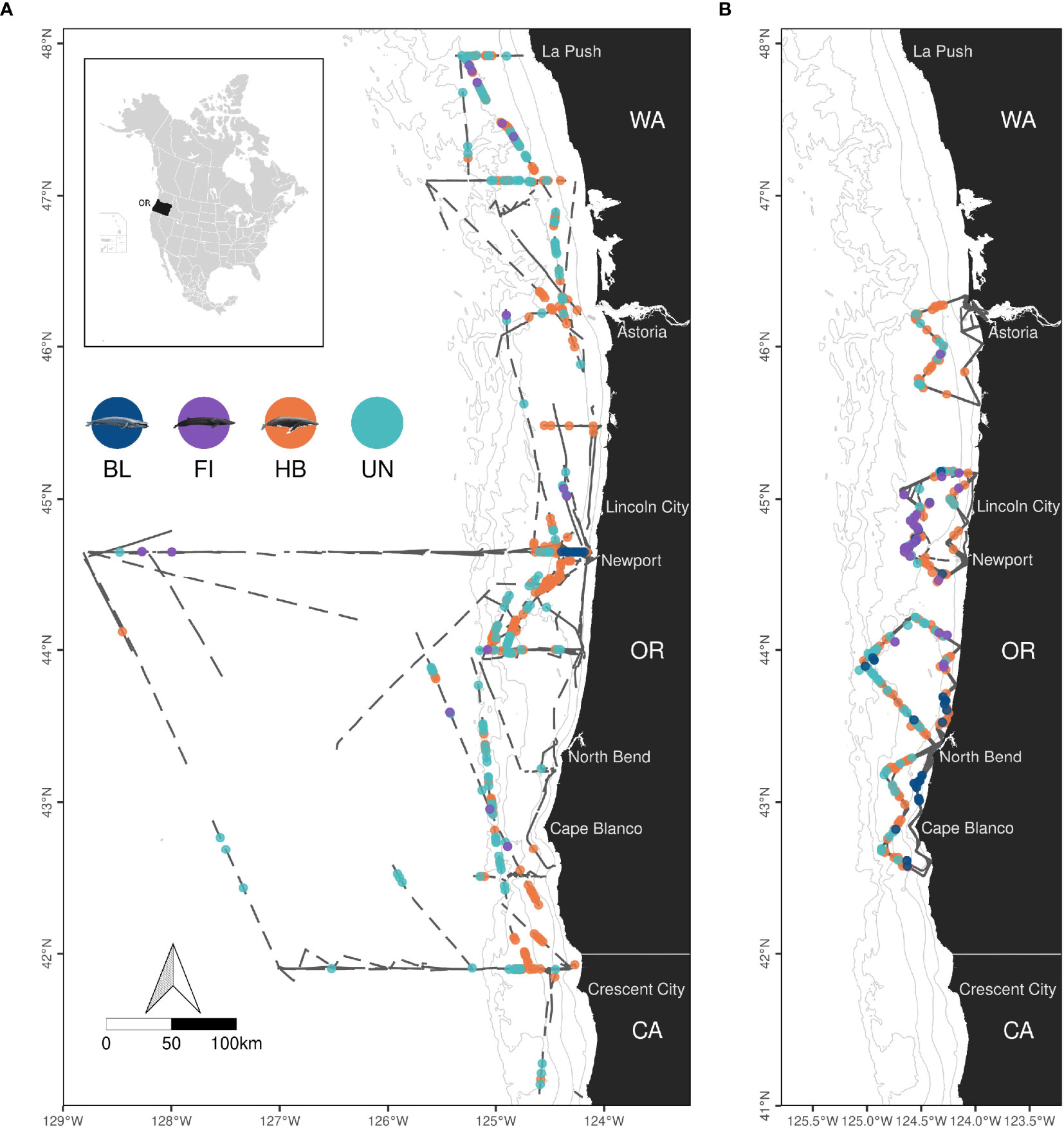
Figure 1 Map of shipboard (A) and helicopter (B) survey effort and observations of rorquals (BL, blue whales; FI, fin whales; HB, humpback whales; UN, Unidentified rorquals) from 2016 to 2021 in Oregon waters (OR), USA. Dark grey lines represent surveyed transect lines in Oregon (OR), California (CA) and Washington (WA) states. Land is shown in black. Isobaths (50, 100, 500, 1,000 and 1,500 m deep) are represented with grey lines. Maps are limited to 41°N but shipboard effort extends south to 37°N. Credits for whale illustrations: Frédérique Lucas and NOAA Fisheries.

2.1.3 Shipboard Surveys

Cetacean survey data were acquired from two different sets of cruises conducted in Oregon (Figure 1). First, observers were placed on the Northern California Current ecosystem survey cruises (NCC, NOAA/NWFSC) since February 2018 to collect cetacean sightings during transits between oceanographic sampling stations located between La Push (Washington state) and Crescent City, Trinidad or San Francisco (California) and offshore as far as 200 nmi (~ 370 km). NCC cruises are conducted aboard the R/V Bell M. Shimada each February, May and September. During survey effort, the ship traveled at about 10 knots, with occasional sections of effort conducted at 5 knots since 2020 due to other research needs. Observations were strictly conducted in passing mode. Second, several STEM cruises (Science, Technology, Engineering and Mathematics) were conducted in September for educational and scientific purposes aboard the R/V Oceanus. Observations were made in closing mode, with the ship breaking transect to approach cetaceans to allow photo-identification after detection. In general, animals were searched for with naked eye, using binoculars at least 30% of the time. Weather permitting, observations were conducted from the flying bridge located respectively 13 m above the waterline aboard the Shimada and 11 m aboard the Oceanus. Poor survey conditions (rough sea state, rain, or fog) episodically forced observers to move to the bridge (Shimada: 10.5 m high, Oceanus: 8.5 m high). Upon detection of cetacean groups, radial distance was estimated either visually or using marine binocular reticles (Fujinon 7x50’s), species were identified and group size was conservatively estimated. The angle between the trackline and the cetacean group was recorded to later derive perpendicular distance with a simple trigonometric equation.

2.1.4 Environmental Variables

Whale habitat use was assessed with respect to topographic and dynamic environmental variables known to reflect the distribution of whales (Becker et al., 2016; Becker et al., 2018; Abrahms et al., 2019), other marine predators (Brodie et al., 2018) or their prey (Cimino et al., 2020; Muhling et al., 2020) in the CCS. Bathymetric charts were obtained from the General Bathymetric Chart of the Oceans (GEBCO, 15 arc-second resolution). Coastlines were obtained from the OpenStreetMap dataset. Distance to the closest submarine canyon was calculated from a worldwide geomorphological map (Harris et al., 2014). Dynamic variables were acquired from daily fields of the near-real time configuration (2011-present) of the Regional Ocean Modeling System (ROMS, Neveu et al., 2016) covering the CCS from 134°W to the coast, and from 30 to 48°N, with a horizontal resolution of 0.1° (see details and sources in Supplementary Table S1).

Eight variables were derived from ROMS to describe surface and subsurface ocean circulation dynamics: sea surface temperature (SST in °C) and its spatial standard deviation (SSTSD; calculated over 0.3° squares), sea surface height (SSH in m) and its standard deviation (SSHSD; calculated over 0.3° squares), eddy kinetic energy (EKE; calculated from eastward and northward surface current velocities, kg·m²·s⁻²), wind stress curl (CURL in Newton·m^-3), isothermal layer depth (ILD in m) and bulk buoyancy frequency (BBV averaged over the upper 200 m, also known as Brunt-Väisälä frequency, in s^-1, Table S1). Frontal zones and areas of high mesoscale variability showing high SSTSD and SSHSD are hypothesized to concentrate prey and drive whale distribution (Scales et al., 2014; Becker et al., 2016). In addition, low SST combined with low BBV, shallow ILD, and high CURL are indicative of strong wind stress and subsequent water column vertical mixing that occurs during upwelling events in the CCS in spring and summer (Brodie et al., 2018; Abrahms et al., 2019). ROMS daily layers were slightly extrapolated in the most nearshore waters of the study area where data gaps of 0.1° wide were filled with the average values from the three nearest neighboring cells. EKE layers were log10-transformed following Cimino et al. (2020). All environmental layers were projected in a Universal Transverse Mercator coordinate system to ensure accurate spatial computations within our study area (UTM 10N) and rescaled to 5-km resolution to match the scale of survey effort segmentation.

2.1.5 Validation Sightings

Opportunistic sightings collected through citizen science and sightings recorded as part of other research programs were compiled into an independent sighting dataset destined to validate model predictions. Citizen science sightings were mainly recorded with the Whale Alert and Ocean Alert Apps, provided by Point Blue Conservation Science. Research sightings were provided by several institutions and covered a wide time frame, from 1989 to 2021. Sources and metadata are provided in Supplementary Table S2. Position, date, group size and species identification were compiled. Offshore sightings made past the 1,500 m isobaths and potential duplicate sightings were excluded. Citizen science sightings made from land viewpoints were shifted by 0.01° west to be relocated at sea.

Given the large time span of this validation data across 3 decades, we conducted a supplementary analysis comparing the sighting rates of rorqual species across three time periods with similar survey effort: ORWA and DEPLHIN surveys in 1989-1992 (Brueggeman, 1992; Green et al., 1992), PaCSEA surveys in 2011-2012 (Adams et al., 2016), and the present study in 2016-2021. We recognize that these surveys had different designs (Supplementary Table S3). Hence, to compare sighting rates across decades we applied two different methods to account for survey effort:(1) the number of individuals observed was divided by the total distance surveyed (whales/km), and (2) the number of individuals observed within the strip width surveyed was divided by the approximate area surveyed (whales/km²).

2.2 Data Processing

2.2.1 Species Observation and Classification

Upon sightings, group size and cetacean identification at the highest taxonomic level were recorded. As commonly experienced in passing mode surveys, many sightings could only be resolved to the family or genus level (Schwarz et al., 2010). To utilize valuable detections of unidentified baleen whales, we applied a random forest classifier (cforest from R party package version 1.3-7) following Roberts et al. (2016) to classify these sightings into rorquals (humpback, blue or fin) or gray whale (Eschrichtius robustus) groups (see details in Supplementary Material; Figure S1), as gray whales were also observed but have a distinct ecological niche (nearshore, shallow; Darling et al., 1998).

2.2.2 Effective Strip Width

Effective strip width (ESW) was modeled hierarchically across platforms and survey conditions using the approach and custom codes designed by Virgili et al. (2018). Based on the similar size and behavior of the three rorqual species of interest (humpback, blue or fin whales) that affect mean perpendicular distance of detection (Barlow et al., 2001), sightings of these species were pooled to increase sample size and more robustly estimate the detection functions from which ESW could be derived. Hierarchical modeling of rorqual detection functions was performed in a Bayesian framework using JAGS 4.3.0 and the R rjags package (version 4-10). Two separate models were produced for helicopter and shipboard surveys. In the helicopter model, transect (Warrenton, Newport, North-NB, South-NB) was included as a random effect and BSS was included as a covariate (three groups). In the shipboard model, cruise ID was included as a random effect (e.g., NCC cruise September 2021, STEM cruise September 2016, etc.), while covariates included BSS (three groups) and observation height (four categories: Shimada flying bridge and bridge, Oceanus flying bridge and bridge). Detection functions were fit with a hazard key and truncation distances equal to the 95% percentile of the set of perpendicular distances measured from a given platform type.

2.2.3 Survey Segments

To standardize spatial analysis of cetacean sightings relative to environmental variables, survey effort must be segmented into equal distances (Miller et al., 2013). First, on-effort sections of the survey tracks were split into legs of consistent survey conditions (heading +/- 20° and constant BSS for helicopter surveys, constant speed and BSS for shipboard surveys). Short legs of less than 1 minute were removed from the analysis. Next, each of these legs was split into smaller segments of constant length, using an euclidean division, with any remainder added to the last of the leg’s segment. An optimal segment length of 5 km was selected for both helicopter and shipboard surveys based on a trade-off between high spatial resolution appropriate for management applications and limiting the number of segments with zero detections (Becker et al., 2020a). Sightings were linked to their respective 5-km segments to compute the number of individuals observed per segment (sum of individuals across group encountered); measurement error on group size was therefore not accounted for in these rorqual counts per segments (e.g., Virgili et al., 2018; Becker et al., 2020b).

2.3 Species Distribution Models

2.3.1 Availability

Distance sampling of cetaceans typically suffers from undercounting due to visibility biases. Indeed, perception bias occurs when animals are at the surface and available for detection, but observers fail to detect them for a variety of reasons. On the other hand, availability bias is due to animals being missed by observers when they are underwater (Marsh and Sinclair, 1989). This availability bias depends on multiple factors (Barlow, 2015), including the animals’ diving pattern, and the platform height and speed that determine the ‘time window’ during which the animal is within a detectable range. In this study, density estimates were corrected for availability bias but not for perception bias (e.g., humpback whale density estimates; Heide-Jørgensen et al., 2008; Bortolotto et al., 2016), as the sampling design did not allow for the estimation of the latter (e.g., through mark-recapture distance sampling). The probability P_a of a whale being available for detection was calculated for helicopters and ships (moving at 10 or 5 knots), per rorqual species, based on (Laake et al., 1997; Salgado Kent et al., 2012) and described in Supplementary Material. Availability P_awas averaged across all species to estimate overall rorqual availability per platform.

2.3.2 Rorqual Phenology Models

Rorqual counts per segment were modeled in relation to the day of year to estimate migratory occurrence in Oregon. Generalized Additive Models (GAM, Hastie & Tibshirani, 1990) were fitted to the mean number of individuals per segment with a negative binomial distribution and a logarithmic link function, using the mgcv R package (version 1.8-38, Wood, 2011). The models were limited to segments of effort occurring over the Oregon shelf and slope, and included year as a discrete covariate and day of year as a cyclic spline with basis size limited to 3. For fin whales that tend to occur in the winter, the calendar days were shifted to allow a better fit of the cyclic splines around new year’s eve, such that day of year was shifted to begin on July 18 instead of January 1st. The models were fit with an offset equal to segment length multiplied by the number of observers and ESW (on a log scale). Following the approach to combine observations from multiple platforms developed by Virgili et al. (2018), we weighted the helicopter segments with zero sightings by the availability index calculated per rorqual species. This approach effectively allowed the model to account for the lower availability of whales to platforms moving at higher speed and with a shorter detection range (e.g., helicopters). The mean date of the peak in whale density across years was calculated for each species and for all rorquals combined; the date range around the peak that includes 50% of the maximum predicted density is also reported, termed the “half density range”.

2.3.3 Rorqual Density Models

Rorqual counts per segment were modeled in relation to a series of environmental variables extracted at the centroid of each 5-km segment of survey effort. Contrary to the phenology models, the density models included all segments of effort occurring in Oregon waters and beyond (with a small amount of shipboard effort in the southern Washington state waters and northern California waters, see Figure 1). As collinearity among explanatory variables is known to affect a model’s stability (Dormann et al., 2013), we calculated the Pearson coefficients between each pair of variables and removed variables with coefficients > 0.7. Dynamic variables were computed at a weekly scale, with daily values averaged over the 7 days prior to any given survey day included in the data. Three models were fit to the pooled rorqual counts over separate seasons of contrasting whale ecology in the region (Mror-spring: April-July, Mror-summer: August-November, Mror-winter: December-March). These models were fit with 10 explanatory variables: DEPTH, CANYON, SST, SSTSD, SSH, SSHSD, EKE, ILD, CURL, ILD, and BBV. Three species-specific models were also produced over the period of higher whale occurrence, respectively targeting humpback whales (Mhb, April-November), blue whales (Mbl, April-November) and fin whales (Mfi, August-March). In addition to the above-mentioned environmental variables, the Mhb, Mbl, and Mfi models included day of year as an explanatory term to account for phenology in the region. GAMs were applied with the mgcv R package and parametrized as in the phenology models (offset, weights, Restricted Maximum Likelihood). Environmental explanatory variables were modeled with penalized thin‐plate regression splines with basis size limited to 5 to prevent overfitting (Wood, 2017). Variable selection was conducted with a shrinkage approach implemented in the mgcv R package, which adds an extra penalty to each smoother and penalizes non-significant variables to zero (Marra and Wood, 2011). In the species-specific models, the day of year variable was not adjusted with a cyclic regression spline since these models were not fitted on year-round data.

2.3.4 Evaluation and Predictions

Models were run with a 10-folds cross-validation (Roberts et al., 2017) grouped over survey days to account for the hierarchical structure of the data (i.e., segments from the same survey day were not split over multiple folds, Derville et al., 2018). The percentage of deviance explained by each of the 10-fold runs was calculated over the training fold. In turn, each of the 10 folds was used as a test dataset to compute external evaluation of the density models. Model accuracy and discrimination power were respectively assessed by calculating the root of mean square error (RMSE) and the Spearman correlation coefficient (rho) between observed and predicted densities in the test fold (Brodie et al., 2021). The ability of models to accurately predict areas with no whale occurrence was assessed with true negative rates (i.e., proportion of segments with no whales that had predicted densities ≤ 1 whale within the effective area surveyed). Finally, all evaluation metrics were averaged over the 10-folds model runs. Functional response plots were produced for each significant environmental predictor-season combination across folds (approximate smooth term significance with p-value < 0.05) to visualize the effect of one variable while all others were held constant at their mean (Friedman, 2001). Variable importance was estimated as the number of fold runs with approximate significance p-values less than 0.05, 0.01 and 0.001.

Rorqual density was predicted from 2016 to 2021 at monthly scale, on a 5-km resolution grid of Oregon waters < 1,500 m. This spatial scale was selected in accordance with survey effort segmentation and to evaluate whale distribution at a resolution that would facilitate targeted management of human activities on the continental shelf that may interact with whales. For each month, predictions were first computed at a weekly scale, from the last week of the previous month to the third week of the month of interest (e.g., for May predictions, whale densities were predicted over four weeks from April to May 24). Median predicted whale densities were calculated across the 10 cross-validation runs for each week, and were in turn used to calculate the median monthly predicted density layers across 4 weeks. Environmental extrapolation was not limited in the predictions per se, but the areas where environmental conditions strayed outside their training ranges by season were highlighted in the Supplementary Material, as they should be considered with caution (Mannocci et al., 2017; Derville et al., 2018).

2.3.5 Independent Validation

Independent sightings recorded through citizen science and other research surveys were used to validate model outputs. All sightings were projected over the 5-km resolution grid and were grouped per day, per grid cell (i.e., group sizes of sightings occurring within 5 km cells were summed). Since the ROMS environmental layers used to produce the rorqual density models were available beginning in 2011, predictions could be produced at the time and position of sightings recorded from 2011 to 2021. The Mhb, Mbl and Mfi models were used to predict species-specific densities where and when humpback, blue and fin whales were respectively recorded in the validation dataset. The Mror model was used to predict rorqual whale density of all taxa (combined dataset of all rorqual sightings and reclassified unidentified whales via random forest analysis) at all the positions where they were recorded in the validation dataset. Predicted densities were compared to observed densities, allowing for the estimation of discrimination power and true positive rates (i.e., proportion of sightings with predicted densities ≥ 1 whale/grid cell).

Models were further evaluated by calculating the proportion of independent sightings that occurred within monthly hotspots derived from 2016-2021 predictions. Hotspots were considered areas recurrently predicted with high whale densities across the 5 years over which the models were trained. Overall rorqual densities, as well as species-specific densities (humpback, blue, and fin whales) were predicted over all months, from January 2016 to September 2021. Monthly predicted maps were summed together across years and rescaled to 0-100 relative values of habitat suitability. Hotspots were defined as the cells with suitability values within the highest 25% of the distribution. The proportion of independent sightings recorded within these monthly hotspots was calculated as a metric of independent model validation.

All analyses were performed using R statistical computing (R Core Team, 2021).

3 Results

3.1 Temporal Effort and Whale Sightings

Cetacean surveys were conducted across 102 days from helicopters and 75 days from ships, totaling 22,579 km and 5,738 km of effort, respectively (Table 1). Survey effort was generally greater in Aug-Nov, both in terms of distance covered and time on effort. Shipboard survey effort extended further offshore than helicopter surveys and outside Oregon waters for a small part (6% in Washington and California state waters, Figure 1). BSS conditions 2-3 were most common (64% overall).

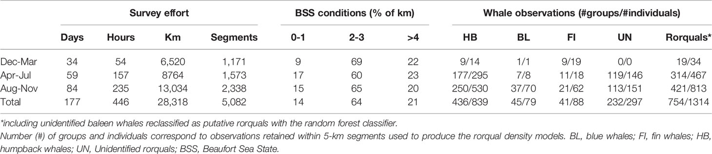
Table 1 Research effort and whale observations from helicopter and shipboard surveys, September 2016 to September 2021.

Most observations were concentrated on the continental shelf, with the exception of a few unidentified baleen whales and several fin whales observed offshore (Figure 1 and maps by species in Supplementary Figures S2–S4). Humpback whales were observed in greatest numbers (426 groups, 839 individuals, Table 1), compared to blue and fin whales. A great number of whale groups could not be identified to species level (269 groups totaling 351 individuals). Among those, 232 groups (86% of groups, totaling 297 individuals) were classified as rorquals a posteriori based on the results of the random forest classifier (Supplementary Figure S5).

The overall independent rorqual sightings dataset was composed of 388 sightings (Supplementary Table S2, Figure S6) representing 886 individual whales aggregated over 273 grid cells of 5 km resolution. Alike the present study, sightings were dominated by humpback whales (190 sightings including 701 individuals), with only a small proportion of blue (38 sightings including 89 individuals) and fin whales (18 sightings including 43 individuals, Table 2). The majority of these observations were collected between April and November (Table 2). They covered a wide time frame, from 1989 to 2021. For the periods 1989-1992 and 2011-2012, independent sightings were all sourced from systematic research surveys comparable in spatio-temporal extent to the present study (Supplementary Figure S7). A temporal comparison of the crude sighting rate calculated over these two periods and the present study revealed a major change in rorqual numbers and species proportions (whales/km in Figure 2), even when effective strip width was accounted for (whales/km² in Supplementary Figure S8). Sighting rates over the Oregon continental shelf and slope multiplied by 17 between the 1989-1992 surveys and the present study. Moreover, the number of blue and fin whales dramatically increased, specifically blue whales that composed only 1% of individuals observed in 1989-1992 (only 1 individual observed), compared to 7% recently.

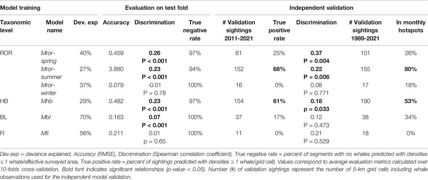
Table 2 Summary of the species density models for rorquals (ROR), humpback whales (HB), blue whales (BL) and fin whales (FI).

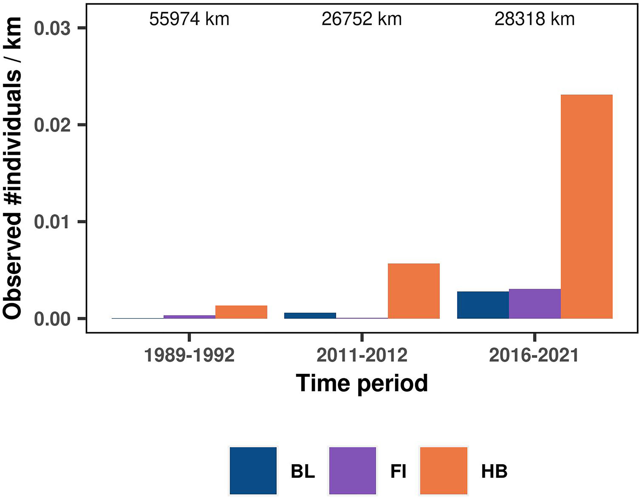
Figure 2 Comparison of the number of individual whales observed per km of effort across systematic research surveys conducted in 1989-1992 (DELPHIN and ORWA marine mammal and seabird surveys), 2011-2012 (PaCSEA surveys) and 2016-2021 (present study). The numbers on top of each bar indicate kilometers surveyed in each period. See Supplementary Tables S2–S3 for more details about systematic research survey data included in the comparison and Supplementary Figure S8 for alternative approach to the sighting rate comparison.

3.2 Multi-Platform Detection

Helicopter and shipboard detection functions were modeled based on 250 and 407 rorqual perpendicular detection distances, respectively (Supplementary Figure S9). The truncation distance was set to 4,690 m for helicopter detections and 9,904 m for shipboard detections based on the 95^th percentile of the sighting perpendicular distances. Detection distances were generally greater for shipboard surveys compared to helicopter surveys. In helicopter surveys, the mean ESW showed little difference across BSS groups, as it only varied from 914 m ± SE 372 m to 1,093 m ± SE 431 depending on BSS conditions (Supplementary Figure S10). In shipboard surveys, the mean ESW varied from 2,073 m ± SE 912 m to 3,217 m ± SE 1,020 m depending on BSS conditions and platform height. As expected, ESW was slightly greater when BSS was lower and when observation height was greater (i.e. from the flying bridge of both ships).

Availability during shipboard surveys was equal to 1 for all three rorqual species and for both vessel speeds experienced during shipboard surveys (10 or 5 knots). On the other hand, availability during helicopter surveys was < 1 and varied between species, between 0.76 for humpback whales, 0.64 for fin whales, and 0.52 for blue whales, as expected from their respective mean dive cycles. The overall rorqual availability during helicopter surveys was estimated at 0.72.

3.3 Whale Phenology in Oregon

Most observations were concentrated in May and September (Figure 3A), due to NCC cruise schedules. Humpback, blue, and fin whales were observed in all three seasons of interest, but in disparate numbers. No fin whales were observed in June, July, nor August, while these months comprised the majority of blue whale sightings. Humpback whales were observed in all months except for January and were most frequent from May to November (Table 1 and Figure 3A). The phenology models identified the peak of density over the Oregon continental shelf and slope as Sep 26 (half density range: Aug 16 to Nov 12) for blue whales, December 18 (half density range: Oct 24 to Feb 18) for fin whales, and August 24 (half density range: Jun 20 to Oct 19) for humpback whales (with deviance explained = 31%, 26% and 15% respectively). Overall the peak of rorqual density was estimated to occur around September 2 (half-strip range: Jun 21 to Nov 13, deviance explained = 9%, Figure 3B).

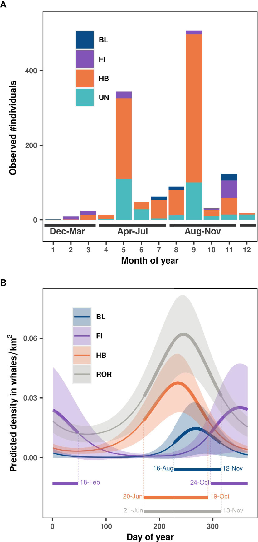
Figure 3 Temporal distribution in (A) observed number of individual whales per month, and (B) predicted whale density estimated over the study region per day of year. BL, blue whales; FI, fin whales; HB, humpback whales; UN, Unidentified rorquals; ROR, all rorquals species pooled together. Season delimitations are represented at the bottom of panel (A). Solid lines represent the marginal effect of day of year on whale density (with year fixed to 2020) and shaded areas represent approximate 95% confidence intervals in panel (B). Half-density ranges representing the peak of occurrence for each species are shown at the bottom of panel (B).

3.4 Whale Habitat Relationships

Seasonal rorqual models were based on 10 environmental variables extracted over 5,082 standardized 5 km segments of effort (Table 1). They revealed different ecological relationships, varying in strength and complexity across seasons (Supplementary Table S4). From December to March (Mror-winter), few environmental variables were able to explain and predict rorqual occurrence (Figure 4A). The prevalence of survey segments with zero observations was reflected in a relatively high deviance explained (37%, Table 2), but weak environmental relationships resulted in poor predictive power across the test folds and when compared to the independent validation dataset (true positive rate was equal to 0). On the other hand, the Mror-spring and Mror-summer models had moderate to high descriptive and predictive power, as reflected in the significant discrimination scores obtained both across the test folds and during independent validation (Table 2). Variable importance (Figure 4A) and functional response plots (Figure 3B) revealed some common habitat selection patterns between these two seasons. ILD was one of the most influential variables in both the Mror-spring and Mror-summer models. Shallow ILD (< 30 m) was associated with higher whale densities. Conversely, SSHSD also strongly influenced rorqual whale densities in both models but with marked seasonal differences, as intermediate values (~ 0.01) were favored in summer vs high values (> 0.03) in spring. Other important variables included DEPTH, SST, SSTSD and CURL in Mror-spring, and SST and BBV in Mror-summer. Low BBV was favored in both models and high SSTSD was preferred in the spring (Figure 4B).

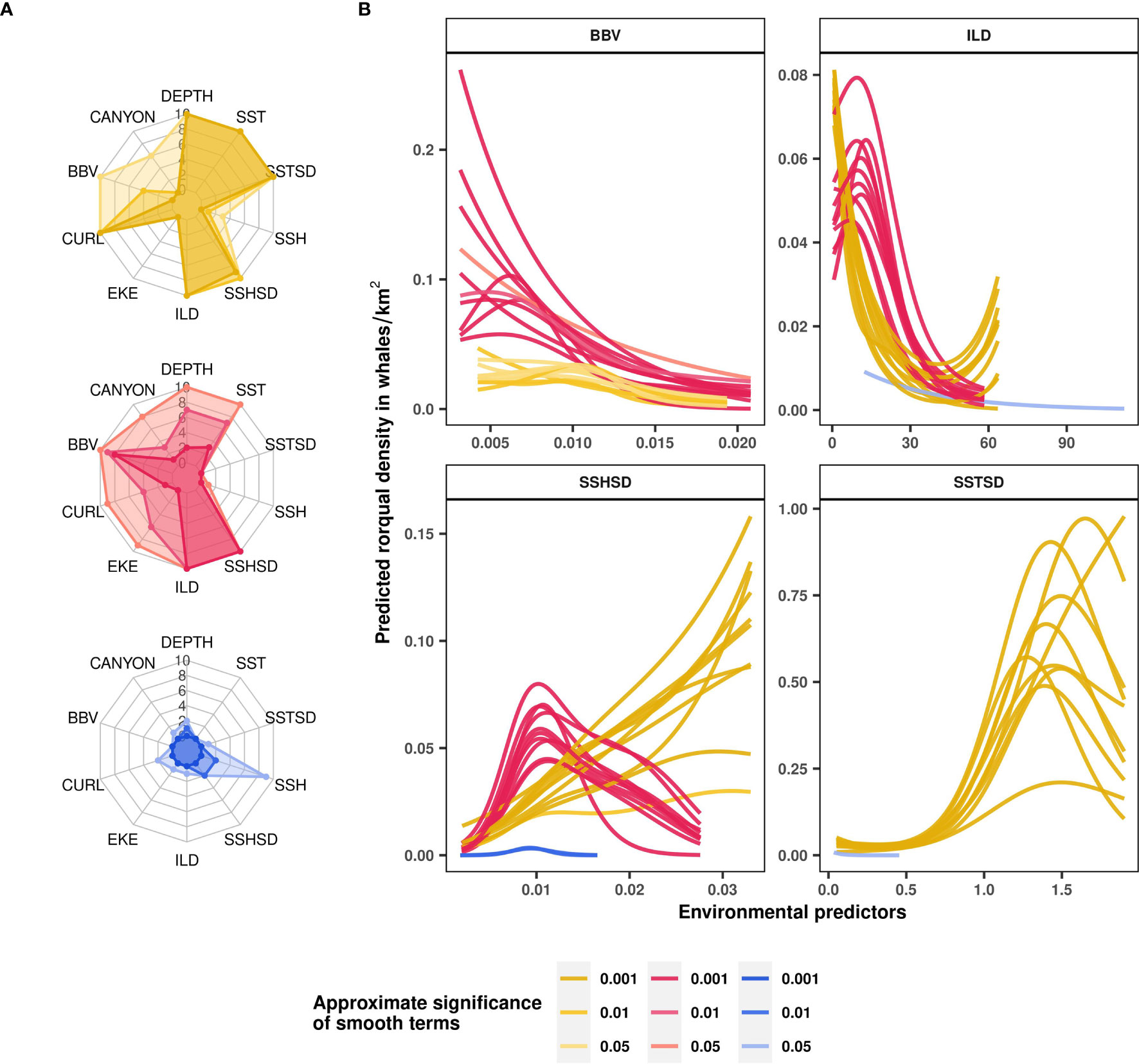
Figure 4 Rorqual ecological relationships modelled over three seasons: April-July (Mror-spring, in yellow), August-November (Mror-summer, in pink) and December-March (Mror-winter, in blue). Variable contributions to rorqual models illustrated as radar plots (A) are measured by the number of cross-validation folds in which the approximate smooth significance p-values were below 0.05, 0.01 or 0.001 (shown with increasingly dark color shades). Functional response curves (B) represent the effect of the smooth function of a selected set of predictor variables (BBV, ILD, SSHSD and SSTSD) upon the trend in rorqual density, with higher values indicating higher predicted densities. Solid lines represent the marginal effect of each variable relative to rorqual density per season and per cross-validation fold. Only the contributors with approximate smooth significance p-value < 0.05 are shown per model fold. Environmental variables: distance to canyons (CANYON in km), seabed depth (DEPTH in m), sea surface temperature (SST in °C) and its spatial standard deviation (SSTSD calculated over 0.3° squares), sea surface height (SSH in m) and its standard deviation (SSHSD calculated over 0.3° squares), eddy kinetic energy (EKE calculated from eastward and northward surface current velocities, kg·m²·s⁻²), wind stress curl (CURL in Newton.m^-3), isothermal layer depth (ILD in m) and bulk buoyancy frequency (BBV in s^-1).

The Mhb, Mbl and Mfi models provided insights into the species-specific ecological relationships of rorquals in Oregon (Supplementary Table S5). Although the Mfi model had a relatively high deviance explained, it performed poorly in the test evaluation and the independent validation (Table 2). On the other hand, the Mhb model had a lower deviance explained but predicted independent sightings better than average (61% true positive rate and discrimination coefficient 0.18, p-value < 0.05). The Mbl model had intermediate performance as it showed significant discrimination power over the test evaluation (coefficient 0.07, p-value < 0.001) but mixed performance in the independent validation.

In line with the rorqual models, ILD was a relatively important contributor to all three of the species-specific habitat models (Figure 5A), highlighting a general preference for waters with shallow ILD (Figure 5B). SST also contributed to humpback, blue, and fin whale models, with higher densities associated with colder waters (< 13°C). Furthermore, blue whales were predicted to occur in greater numbers when BBV was low and when SSHSD was intermediate (~0.01). Fin whale densities were predicted to be particularly higher in proximity to canyons. The Mfi relationship to DEPTH was sensitive to the cross-validation as the different fold runs showed different functional responses that highlighted the importance of deep and offshore waters up to 2,500 m deep.

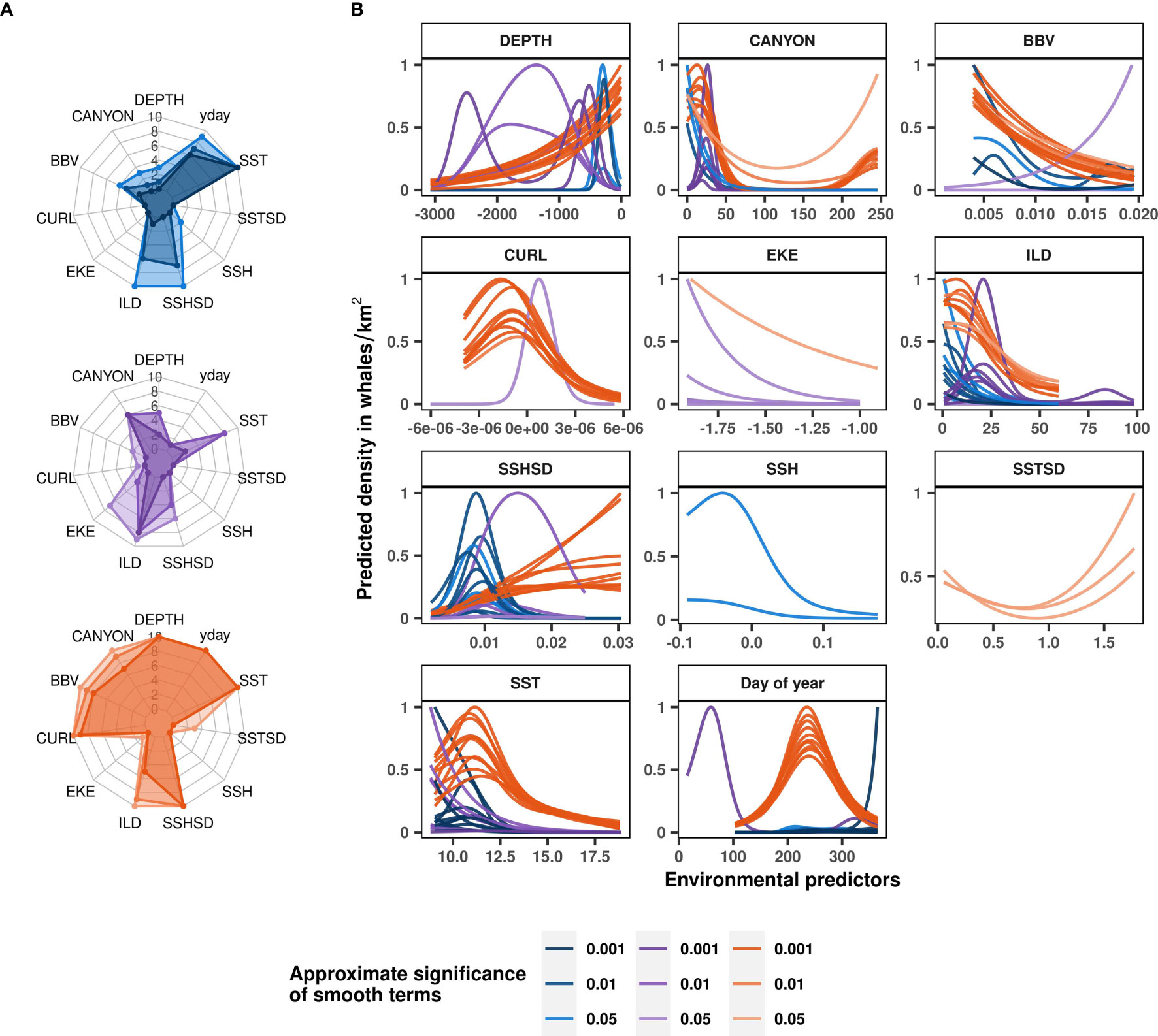
Figure 5 Blue, fin and humpback whale ecological relationships modelled with Mbl (in blue), Mfi (in purple) and Mhb (in orange) respectively. Variable contributions to species-specific models illustrated as radar plots (A) are measured by the number of cross-validation folds in which the approximate smooth significance p-values were below 0.05, 0.01 or 0.001 (shown with increasingly dark color shades). Functional response curves (B) represent the effect of the smooth function of environmental variables upon the trend in rorqual density, with higher values indicating higher predicted densities. Solid lines represent the marginal effect of each variable relative to whale density per cross-validation fold. Only the contributors with approximate smooth significance p-value < 0.05 are shown per model fold. Environmental variables: day of year (yday), distance to canyons (CANYON in km), seabed depth (DEPTH in m), sea surface temperature (SST in °C) and its spatial standard deviation (SSTSD calculated over 0.3° squares), sea surface height (SSH in m) and its standard deviation (SSHSD calculated over 0.3° squares), eddy kinetic energy (EKE calculated from eastward and northward surface current velocities, kg·m²·s⁻²), wind stress curl (CURL in Newton.m^-3), isothermal layer depth (ILD in m) and bulk buoyancy frequency (BBV in s^-1).

Finally, the Mhb model was relatively similar to the Mror-spring and Mror-summer models, as expected from the dominance of humpback whales in rorqual species observed off the Oregon coast (Figure 3A). SSHSD, SST, day of year, DEPTH, CURL, BBV, distance to canyons and ILD had a significant effect on humpback whale densities in almost all of the cross-validation runs (Figure 5A). The Mhb model generally showed a preference of humpback whales for high SSHSD, low BBV and low CURL. The relationship with distance to canyon was bimodal, with a marked preference for waters closer to canyons (< 50 km). Humpback whales densities increased with decreasing seabed depth, with a faint inflexion around 1,000 m deep corresponding to the limit of the continental shelf.

3.5 Predicted Density Patterns

Predictive maps of rorqual densities (Figure 6) were produced for the months of interest (January, May and September) corresponding to each seasonal model (Mror-winter, Mror-spring and Mror-summer respectively). The seasonal migratory behavior of rorquals was clearly reflected in these predictions, whereby densities across the majority of the study area were generally predicted to be low in January, increase through May, and be the highest in September. In comparison to other months, predicted densities in January were very low across the Oregon shelf and slope. Densities increased in May, specifically over a few discrete hotspots located on the continental slope and varying across years. In September, densities peaked and were predicted to be the highest on the continental shelf, off Cape Blanco, North Bend and Newport. Over all seasons, densities were predicted to be low in nearshore, shallow waters (< 50 m deep), with the exception of the nearshore waters south of Cape Blanco where rorquals are predicted to occur in relatively high numbers in September.

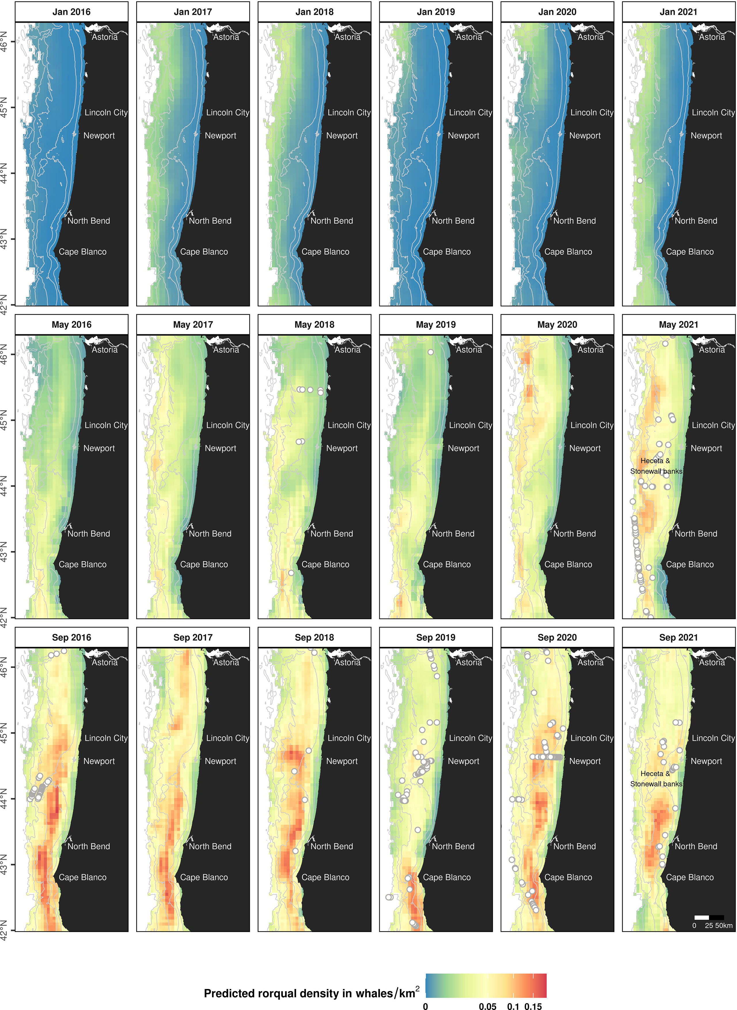
Figure 6 Predicted seasonal densities of rorqual whales for the months of January, May and September, 2016 to 2021. Densities are represented on a colored scale (square-root transformed gradient). Land is shown in black. Isobaths (50, 100, 500, 1,000 and 1,500 m deep) are represented with grey lines. Grey circles mark the position of observed rorqual groups during each month x year from shipboard and helicopter surveys used to train the models. The absence of observations may be due to an absence of survey effort. This figure is also available in a color-blind-friendly palette in Supplementary Figure S18).

Species-specific maps of predicted densities provided further insights into the spatio-temporal patterns of occurrence of rorqual species (Supplementary Figures S11–S13). On average across years, humpback whale hotspots were mostly predicted to be over the continental shelf and slope waters deeper than 50-100 m, whereas blue whale distribution extended more inshore and was limited to the southern part of the study region (Figure 7 and Supplementary Figures S14–S17). The percent of overlap between monthly hotspots and sightings recorded independently since 1989 was higher for humpback (53%) than blue whales (34%, Table 2). Overall, hotspots derived from the rorqual Mror-summer model predictions had the best overlap with independent sightings (80%), as illustrated in the September hotspot map (Figure 7).

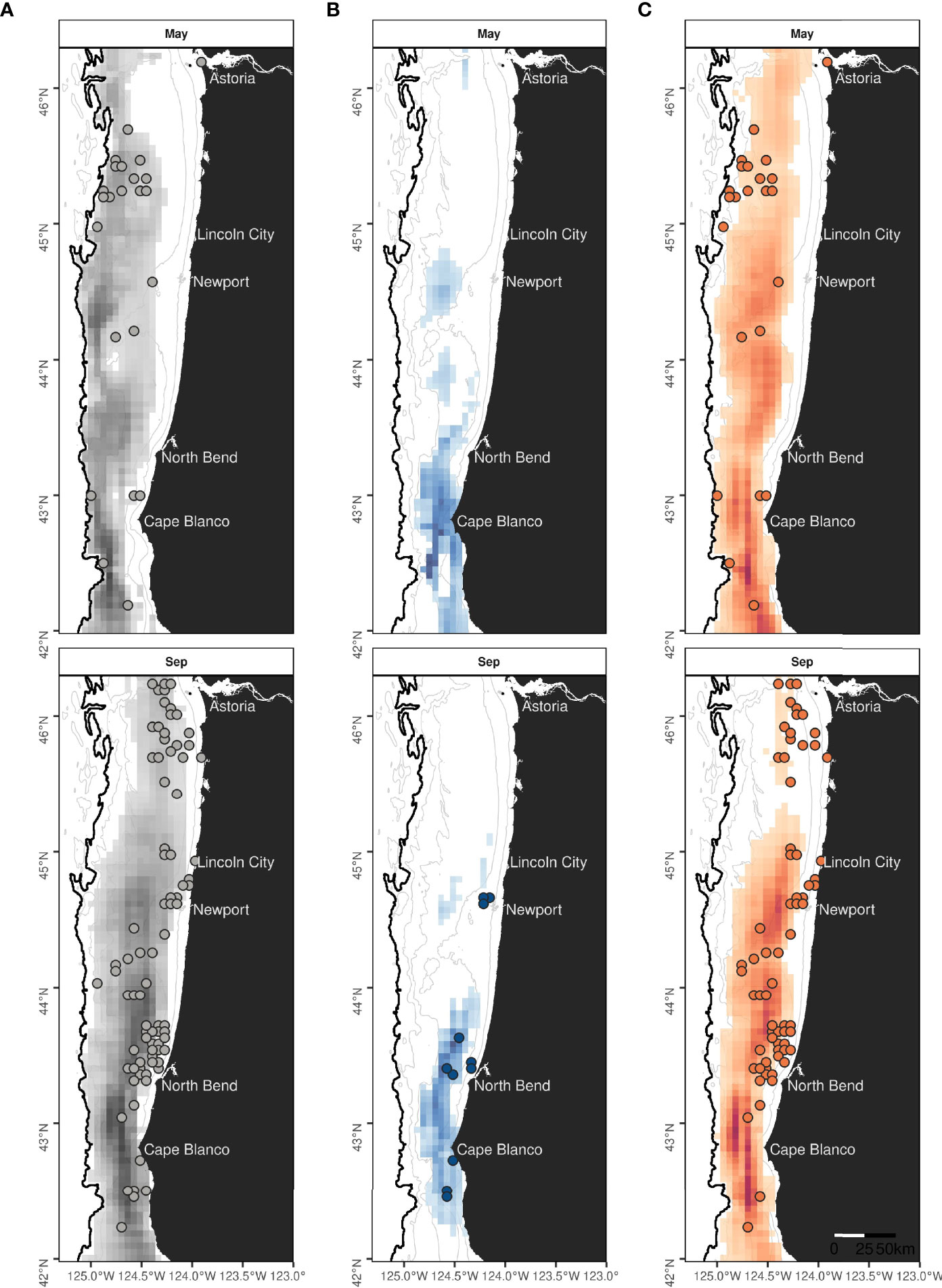
Figure 7 Monthly hotspots predicted over 2016-2021 for rorquals (A), blue (B) and humpback whales (C) in May and September. The best 75% of the summed and rescaled densities are represented on species-specific colored scales. Land is shown in black. Isobaths (50, 100, 500 and 1,000 m deep) are represented with grey lines. Colored circles mark the position of independent validation sightings of rorquals, blue, or humpback whales recorded in May or September, of 1989 to 2021 (see Supplementary Table S2 for data sources and details). The absence of observations may be due to an absence of survey effort.

4 Discussion

Balancing expanding human activities in the ocean and protection of biodiversity is a challenge. Informed spatial management through a highly resolved understanding of biodiversity distribution patterns can alleviate some conflicts. In this study, we collected and analyzed year-round whale occurrence data across Oregon shelf waters, demonstrating (1) an increase in rorqual whale numbers over the last three decades, (2) differences in timing of migration and habitat preferences across humpback, blue, and fin whales, and (3) predictable relationships between rorqual whale distribution and dynamic ocean conditions indicative of upwellings and frontal zones. These findings illustrate that more rorqual whales now occur in Oregon waters than previously, requiring modern data assessed within a dynamic ocean framework to support conservation efforts. This study provides up-to-date predictions of rorqual whale densities at a fine spatio-temporal scale that is relevant to the spatial management of human activities in Oregon.

Historical comparison of sighting rates across the last three decades revealed an overall increase in rorqual numbers in Oregon. Compared to aerial surveys conducted in 1989-1992 (Brueggeman, 1992; Green et al., 1992), humpback, blue, and fin whales are now more abundant, with humpback whales being by far the most common rorqual species observed in Oregon overall. These trends align with population increases of humpback and fin whales at the scale of the US West Coast described through mark-recapture and aerial surveys respectively (Barlow et al., 2011; Moore and Barlow, 2011; Calambokidis et al., 2017; Calambokidis and Barlow, 2020). Blue whales in the CCS, however, only showed slight signs of increase since the 1990s (Calambokidis and Barlow, 2020), as the eastern North Pacific stock that migrates and feeds off the US West Coast is believed to have reached carrying capacity (Monnahan et al., 2015). Yet, it has been suggested that the distribution of this blue whale population has shifted northward or undergone a range expansion during the same period (Calambokidis et al., 2009). We provide more evidence of an increased use of northern CCS waters by blue whales over the last three decades. The nature, drivers and time frame of this distribution change are unclear, although blue whales are hypothesized to migrate further north in response to environmental changes influencing prey availability (Bailey et al., 2009; Calambokidis et al., 2009).

Our density models indicate that rorqual whales off Oregon prefer habitat with low BBV, shallow ILD, and low SST conditions, characteristics typical of highly mixed and cold nearshore upwelled waters (Brodie et al., 2018; Anglès et al., 2019; Nampoothiri et al., 2020). Moreover, the selection for high SSTSD and SSHSD indicates a preference for frontal oceanographic areas and areas of high mesoscale variability (Scales et al., 2014; Becker et al., 2016). These physical conditions are assumed to provide suitable biological conditions for increased prey abundance and correspond to results of blue whale habitat use models derived from satellite tracking at the scale of the US West Coast (Abrahms et al., 2019). Yet, the exact timing between upwellings to enhanced biological productivity and whale abundance is not exactly known. Unlike previous studies of whale distribution in the CCS that modeled whale response to daily changes of ocean physical variables (Hazen et al., 2017; Becker et al., 2018; Abrahms et al., 2019; Becker et al., 2020b), we modeled environmental conditions at a weekly scale before the day of surveys. In this way, we assume that whales do not respond instantaneously to ocean physical changes, especially in wind-driven upwelling systems. Blue whales occurrence in an upwelling system in New Zealand have a 3 week lag from wind events that drive productivity on that foraging ground (Barlow et al., 2021), allowing forecasts of blue whale distribution for conservation management applications (Barlow and Torres, 2021). In the CCS, forage species also respond to weekly scale wind variations whereby their aggregation patterns become more discrete and concentrated during periodic upwelling events (Benoit-Bird et al., 2019). In addition to the general seasonal pattern of upwelling that lead to the occurrence of foraging whales months after the peak in primary productivity has occurred (Croll et al., 2005), the within-season variability of upwelling conditions and prey availability also appears to play an important role in driving rorqual whale distribution in the CCS. Moreover, seabed topography is known to interact and locally influence ocean productivity. In this study, the proximity to submarine canyons generally contributed to higher habitat suitability, likely due to the role of canyons as krill hotspots in the CCS (Santora et al., 2018), including in canyons off Cape Blanco that overlap with predicted suitable habitat for blue whales, humpback whales, and rorquals in general (Figures 6, 7). The Heceta and Stonewall banks were also recurrently predicted as a hotspot of rorqual occurrence in summer and fall. These topographic features generate a known retention area with high surface primary productivity (Barth et al., 2005; Gan and Allen, 2005; Hickey and Banas, 2008) that is both an important fishing location (Tissot et al., 2008) and a zone where humpback whales were frequently observed in previous transect surveys over the Oregon continental shelf (Tynan et al., 2005), currently identified as a ‘Biologically Important Area’ for humpback whales (Calambokidis et al., 2015).

Our investigation of species-specific phenology and habitat use highlighted temporal, environmental, and spatial segregation across rorqual species in Oregon. The habitat selection patterns predicted by our locally trained density models aligned well with previous work at broader scales in the CCS (Barlow et al., 2009; Forney et al., 2012; Becker et al., 2020b). Humpback whales were the most spatially and temporally widespread, likely due to their generalist and flexible diet (Pauly and Trites, 1998; Fleming et al., 2016). They showed a preference for the continental shelf and slope, as predicted by US coast-wide (Becker et al., 2018; Becker et al., 2020b) and southern California (Becker et al., 2017) density models derived from ship-based surveys. Their presence was tightly associated with the seasonal upwelling, as reflected in their preference for turbulent, mixed, and surface-cold waters. Blue whales also appeared in Oregon in relation to upwelling, although their presence peaked later in the season compared to humpback whales, which is a temporal pattern similar to that identified in Monterey Bay, California (Fossette et al., 2017). Interestingly, blue whales used shallower waters than humpback whales, as they were constrained to the continental shelf, which corresponds with other blue whale habitat predictions (Barlow et al., 2009; Forney et al., 2012; Becker et al., 2018; Abrahms et al., 2019; Becker et al., 2020b) and with area restricted search identified in blue whale satellite tracks (Bailey et al., 2009; Palacios et al., 2019) in nearshore southern Oregon. However, US west coast-wide models by Abrahms et al. (2019) also predicted relatively high habitat suitability for blue whales in deeper waters just off the continental slope in central Oregon, which our models did not predict. Given that most of the blue whales included in Abrahms et al. (2019) were tagged and tracked in California, we hypothesize that the resulting model predictions are biased towards California habitat drivers that may not apply as well to the northern CCS. Indeed, the nearshore habitat selection pattern we predicted off the coast of Oregon further contrasts with blue whale distribution off southern California where predicted suitable habitats extend far offshore (Barlow et al., 2009; Forney et al., 2012; Becker et al., 2018; Abrahms et al., 2019; Becker et al., 2020b). These dissimilarities emphasize the value of acquiring refined and local whale data to specifically understand distribution patterns and ecological relationships in Oregon waters in support of a more resolved state-wide spatial management. In California, blue whales are known to feed on krill Thyssanoessa spinifera in shallow environments (<100 m water depth) and Euphausia pacifica in shelf-edge and open-ocean environments (Fiedler et al., 1998; Becker et al., 2018). Given that Thysanoessa spinifera has the highest potential energetic content, we hypothesize that blue whales specifically target this krill species in inshore waters of the Oregon shelf (Nickels et al., 2018), particularly in late summer/early fall when the carbon and lipid content of this krill species is at its peak (Fisher et al., 2020). Indeed, blue whales’ preferences for low SST and shallow ILD mirrored the habitat use patterns of Thysanoessa spinifera in the CCS (Cimino et al., 2020).

Despite models including comparable numbers of individual observations, the fin whale model’s predictive performance was lower than that of blue whales. This difference may be explained by the relatively smaller and more restricted niche occupied by blue whales as krill specialists (Fossette et al., 2017). In comparison, the broad-scale movements of fin whales across the North Pacific diverges from the typical baleen whale migration connecting low-latitude breeding areas and high-latitude feeding areas (Mizroch et al., 2009). Fin whales tracked in the CCS showed great individual variability in space use, high residency to localized areas, and when modeled suggested that in summer, Oregon offshore waters are more favorable to fin whales than waters of the continental shelf, while this pattern reverses in winter (Scales et al., 2017b). These predictions align with the phenology and space use by fin whales highlighted in our study, including observations up to 200 nmi offshore in May and large concentrations (max group size = 25 individuals) over the shelf between October and February. These complex patterns may be related to the diverse and flexible diet of fin whales, which feed on both euphausiids and small fish, such as northern anchovy Engraulis mordax and Pacific sardines Sardinops sagax in the CCS (Pauly and Trites, 1998; Mizroch et al., 2009). Overall, the wide depth range that fin whales are predicted to use aligns with predicted occurrence patterns from previous coast-wide models derived from satellite tracking (Scales et al., 2017b) and shipboard surveys that more consistently and intensively surveyed offshore waters (Barlow et al., 2009; Forney et al., 2012; Becker et al., 2018; Becker et al., 2020b).

Our habitat models were designed to scientifically inform management, hence warranting robust predictive performance. The blue whale and fin whale models were ecologically informative and offered promising insights into the phenology and habitat preferences of these rare species. However, these species-specific models showed low predictive performance due to a small sample size, as measured by cross-validation and independent validation with an external observation dataset. As observation data continues to be consistently collected off the Oregon coast through sustained partnerships and local collaborations, we hope that fine-scale habitat use models of these endangered and threatened populations can be improved in the long-term. On the other hand, we consider that the rorqual summer and spring models, and the humpback whale models have reached a level of robustness sufficient to improve predictions of spatio-temporal habitat use in Oregon waters. Although these models were not specifically generated for abundance estimation (due to lack of correction for measurement error in group size and perception bias that will lead to underestimated abundance), these models can be used to predict relative spatio-temporal variations in whale densities to underpin spatial planning and risk assessment. For instance, models were used to locate average hotspots of higher suitability over multiple years (Figure 7 and Supplementary Figures S13–16), hence providing static spatial products to support conservation plans in Oregon (e.g., PrediWhales, Virgili et al., 2018). Additionally, because models were generated using predictor data over the previous seven day period, the outputs can derive near real-time predictions of whale densities to assess daily risks of interactions with human activities. A similar approach is successfully implemented to minimize bycatch of sea turtles in the central North Pacific Ocean (i.e. TurtleWatch, Howell et al., 2015). Finally, models can hindcast whale distribution over multiple years and seasons to retrospectively understand the factors influencing the risks of deleterious interactions with anthropogenic activities. Indeed, cross-correlating time series of whale distribution with fishing activity and with local (e.g., SST, Upwelling Index) and basin-scale climate factors influencing prey availability (e.g., Southern Oscillation Index, Pacific Decadal Oscillation), proved insightful to understanding the increase in whale entanglement rates over the US West Coast (Santora et al., 2020; Feist et al., 2021; Ingman et al., 2021). Therefore, SDMs produced in this study are not considered an end point, but rather a stepping stone to multi-faceted ecological knowledge and operational outputs that will support informed and dynamic management of whales in a changing environment off the Oregon coast.

Data Availability Statement

The data supporting the conclusions of this article are available via the Figshare Digital Repository: https://doi.org/10.6084/m9.figshare.19643355.v1.

Author Contributions

LT acquired funding, conceived and designed the project; CH, LT and DB collected the data; SD and DB processed the data, SD performed the analysis; SD and LT wrote the manuscript; all authors critically reviewed the manuscript. All authors contributed to the article and approved the submitted version.

Funding

This research received financial support from the NOAA Species Recovery Grant (#NA19NMF4720109), the Oregon Dungeness Crab Commission, the Marine Mammal Institute, the Oregon Department of Fish & Wildlife (ODFW) and Oregon Sea Grant.

Conflict of Interest

The authors declare that the research was conducted in the absence of any commercial or financial relationships that could be construed as a potential conflict of interest.

Publisher’s Note

All claims expressed in this article are solely those of the authors and do not necessarily represent those of their affiliated organizations, or those of the publisher, the editors and the reviewers. Any product that may be evaluated in this article, or claim that may be made by its manufacturer, is not guaranteed or endorsed by the publisher.

Acknowledgments

We gratefully acknowledge the immense contribution of the United State Coast Guard sectors North Bend and Columbia River who facilitated and piloted our helicopter surveys. We thank the R/V Bell M. Shimada (chief scientists J. Fisher and S. Zeman) and R/V Oceanus crews, as well as the marine mammal observers F. Sullivan, C. Bird and R. Kaplan. We give special recognition and thanks to the late Alexa Kownacki who contributed so much in the field and to our lives. We also thank T. Buell and K. Corbett (ODFW) for their partnership over the OPAL project. We thank G. Green and J. Brueggeman (Minerals Management Service), J. Adams (US Geological Survey), J. Jahncke (Point blue Conservation), S. Benson (NOAA-South West Fisheries Science Center), and L. Ballance (Oregon State University) for sharing validation data. We thank J. Calambokidis (Cascadia Research Collective) for sharing validation data and for logistical support of the project. We thank A. Virgili for sharing advice and custom codes to produce detection functions.

Supplementary Material

The Supplementary Material for this article can be found online at: https://www.frontiersin.org/articles/10.3389/fmars.2022.868566/full#supplementary-material

References

Abrahms B., Welch H., Brodie S., Jacox M. G., Becker E. A., Bograd S. J., et al. (2019). Dynamic Ensemble Models to Predict Distributions and Anthropogenic Risk Exposure for Highly Mobile Species. Divers. Distrib. 25, 1182–1193. doi: 10.1111/ddi.12940
Adams J., Felis J., Mason J. W., Takekawa J. Y. (2014). “Pacific Continental Shelf Environmental Assessment (PaCSEA): Aerial Seabird and Marine Mammal Surveys Off Northern California, Oregon, and Washington 2011–2012,” U.S. Dept. Of the Interior, Bureau of Ocean Energy Management, Pacific OCS Region (Camarillo, CA: OCS Study BOEM 2014-003). p. 266.
Adams J., Felis J., Mason J. W., Takekawa J. Y. (2016). Pacific Continental Shelf Environmental Assessment (PaCSEA): Aerial Seabird and Marine Mammal Surveys Off Northern California, Oregon, and Washington 2011-2012. Resour. Database U.S. Geol. Surv. Data Release. doi: 10.5066/F7668B7V
Albouy C., Delattre V., Donati G., Frölicher T. L., Albouy-Boyer S., Rufino M., et al. (2020). Global Vulnerability of Marine Mammals to Global Warming. Sci. Rep. 10, 1–12. doi: 10.1038/s41598-019-57280-3
Anglès S., Jordi A., Henrichs D. W., Campbell L. (2019). Influence of Coastal Upwelling and River Discharge on the Phytoplankton Community Composition in the Northwestern Gulf of Mexico. Prog. Oceanogr. 173, 26–36. doi: 10.1016/j.pocean.2019.02.001
Austin M. P. (2007). Species Distribution Models and Ecological Theory: A Critical Assessment and Some Possible New Approaches. Ecol. Modell. 200, 1–19. doi: 10.1016/j.ecolmodel.2006.07.005
Bailey H., Mate B. R., Palacios D. M., Irvine L., Bograd S. J., Costa D. P. (2009). Behavioural Estimation of Blue Whale Movements in the Northeast Pacific From State-Space Model Analysis of Satellite Tracks. Endanger. Species. Res. 10, 93–106. doi: 10.3354/esr00239
Barlow J. (2015). Inferring Trackline Detection Probabilities, G(0), for Cetaceans From Apparent Densities in Different Survey Conditions. Mar. Mammal. Sci. 31, 923–943. doi: 10.1111/mms.12205
Barlow J. P. (2016). Cetacean Abundance in the California Current Estimated From Ship-Based Line-Transect Surveys in 1991-2014. NOAA. Fish. Sci. Cent. Adm. Rep. LJ-16-01, 63.
Barlow J., Calambokidis J., Falcone E. A., Baker C. S., Burdin A. M., Clapham P. J., et al. (2011). Humpback Whale Abundance in the North Pacific Estimated by Photographic Capture-Recapture With Bias Correction From Simulation Studies. Mar. Mammal. Sci. 27, 793–818. doi: 10.1111/j.1748-7692.2010.00444.x
Barlow J., Ferguson M. C., Becker E. A., Redfern J. V. (2009). “Predictive Modeling of Marine Mammal Density From Existing Survey Data and Model Validation Using Upcoming Surveys,” Final Report SERDP Project SI-1391, National Marine Fisheries Service.
Barlow J., Gerrodette T., Forcada J. (2001). Factors Affecting Perpendicular Sighting Distances on Shipboard Line-Transect Surveys for Cetaceans. J. Cetacean. Res. Manage. 3, 201–212.
Barlow D. R., Klinck H., Ponirakis D., Garvey C., Torres L. G. (2021). Temporal and Spatial Lags Between Wind, Coastal Upwelling, and Blue Whale Occurrence. Sci. Rep., 1–10. doi: 10.1038/s41598-021-86403-y
Barlow D. R., Torres L. G. (2021). Planning Ahead: Dynamic Models Forecast Blue Whale Distribution With Applications for Spatial Management. J. Appl. Ecol. 58, 2493–2504. doi: 10.1111/1365-2664.13992
Barth J. A., Pierce S. D., Castelao R. M. (2005). Time-Dependent, Wind-Driven Flow Over a Shallow Midshelf Submarine Bank. J. Geophys. Res. C. Ocean. 110, C10S05. doi: 10.1029/2004JC002761
Becker E. A., Carretta J. V., Forney K. A., Barlow J., Brodie S., Hoopes R., et al. (2020a). Performance Evaluation of Cetacean Species Distribution Models Developed Using Generalized Additive Models and Boosted Regression Trees. Ecol. Evol. 10 (12), 5759–5784. doi: 10.1002/ece3.6316
Becker E. A., Foley D. G., Forney K. A., Barlow J., Redfern J. V., Gentemann C. L. (2012). Forecasting Cetacean Abundance Patterns to Enhance Management Decisions. Endanger. Species. Res. 16, 97–112. doi: 10.3354/esr00390
Becker E., Forney K., Fiedler P., Barlow J., Chivers S., Edwards C., et al. (2016). Moving Towards Dynamic Ocean Management: How Well Do Modeled Ocean Products Predict Species Distributions? Remote Sens. 8, 149. doi: 10.3390/rs8020149
Becker E. A., Forney K. A., Miller D. L., Fiedler P. C., Barlow J., Moore J. E. (2020b). “Habitat-Based Density Estimates for Cetaceans in the California Current Ecosystem Based on 1991-2018 Survey Data,” U.S. Department of Commerce, NOAA Technical Memorandum NMFS-SWFSC-638. Available at: https://ntrl.ntis.gov/NTRL/.
Becker E. A., Forney K. A., Redfern J. V., Barlow J., Jacox M. G., Roberts J. J., et al. (2018). Predicting Cetacean Abundance and Distribution in a Changing Climate. Divers. Distrib. 25, 626–643. doi: 10.1111/ddi.12867
Becker E. A., Forney K. A., Thayre B. J., Debich A., Campbell G. S., Whitaker K., et al. (2017). Habitat-Based Density Models for Three Cetacean Species Off Southern California Illustrate Pronounced Seasonal Differences. Front. Mar. Sci. 4. doi: 10.3389/fmars.2017.00121
Benoit-Bird K. J., Waluk C. M., Ryan J. P. (2019). Forage Species Swarm in Response to Coastal Upwelling. Geophys. Res. Lett. 46, 1537–1546. doi: 10.1029/2018GL081603
BOEM (2021a). “Notice of Research Lease Issuance for Marine Hydrokinetic Energy on the Pacific Outer Continental Shelf Offshore Oregon,” Bureau of Ocean Energy Management, Department of the Interior, Federal Register BOEM-2021-018. doi: 10.1016/0196-335x(80)90058-8
BOEM (2021b). Oregon Offshore Renewable Energy Fact Sheet: BOEM-Oregon Offshore Wind Planning Efforts (Bureau of Ocean Energy Management). Available at: https://www.boem.gov/renewable-energy/state-activities/Oregon.
Bograd S. J., Schroeder I., Sarkar N., Qiu X., Sydeman W. J., Schwing F. B. (2009). Phenology of Coastal Upwelling in the California Current. Geophys. Res. Lett. 36, 1–5. doi: 10.1029/2008GL035933
Bortolotto G. A., Danilewicz D., Andriolo A., Secchi E. R., Zerbini A. N. (2016). Whale, Whale, Everywhere: Increasing Abundance of Western South Atlantic Humpback Whales (Megaptera Novaeangliae) in Their Wintering Grounds. PloS One 11, e0164596. doi: 10.1371/journal.pone.0164596
Brodie S., Abrahms B., Bograd S. J., Carroll G., Hazen E. L., Muhling B. A., et al. (2021). Exploring Timescales of Predictability in Species Distributions. Ecography. (Cop.)., 44 (6), 832–844. doi: 10.1111/ecog.05504
Brodie S., Jacox M. G., Bograd S. J., Welch H., Dewar H., Scales K. L., et al. (2018). Integrating Dynamic Subsurface Habitat Metrics Into Species Distribution Models. Front. Mar. Sci. 5. doi: 10.3389/fmars.2018.00219
Brueggeman J. (1992). Final Report: Oregon and Washington Marine Mammal and Seabird Surveys (Prepared for Pacific OCS Region Minerals Management Service, US Department of Interior, Los Angeles, California).
Buckland S. T., Rexstad E. A., Marques T. A., Oedekoven C. S. (2015). Distance Sampling: Methods and Applications - Methods in Statistical Ecology. (Sptringer International Publishing, Switzerland). doi: 10.1007/978-3-319-19219-2
Calambokidis J., Barlow J. (2020). “Updated Abundance Estimates for Blue and Humpback Whales Along the U.S. West Coast Using Data Through 2018. U.S,” Department of Commerce, NOAA Technical Memorandum NMFS-SWFSC-634. Available at: https://repository.library.noaa.gov/view/noaa/27104.
Calambokidis J., Barlow J., Flynn K., Dobson E., Steiger G. H. (2017). “Update on Abundance, Trends, and Migrations of Humpback Whales Along the U.S. West Coast,” SC/A17/NP/13, Report to the Scientific Committee of the International Whaling Commission. (Bled, Slovenia).
Calambokidis J., Barlow J., Ford J. K. B., Chandler T. E., Douglas A. B. (2009). Insights Into the Population Structure of Blue Whales in the Eastern North Pacific From Recent Sightings and Photographic Identification. Mar. Mammal. Sci. 25, 816–832. doi: 10.1111/j.1748-7692.2009.00298.x
Calambokidis J., Fahlbusch J. A., Szesciorka A. R., Southall B. L., Cade D. E., Friedlaender A. S., et al. (2019). Differential Vulnerability to Ship Strikes Between Day and Night for Blue, Fin, and Humpback Whales Based on Dive and Movement Data From Medium Duration Archival Tags. Front. Mar. Sci. 6. doi: 10.3389/fmars.2019.00543
Calambokidis J., Steiger G. H., Curtice C., Harrison J., Ferguson M. C., Becker E., et al. (2015). Biologically Important Areas for Selected Cetaceans Within U.S. Waters – West Coast Region. Aquat. Mamm. 41, 39–53. doi: 10.1578/AM.41.1.2015.1
Carretta J. V., Forney K. A., Oleson E. M., Weller D. W., Aimee R., Baker J., et al. (2021). “U.S. Pacific Marine Mammal Stock Assessments: 2020,” U.S. Department of Commerce, NOAA Technical Memorandum NMFS-SWFSC-646.
Cimino M. A., Santora J. A., Schroeder I., Sydeman W., Jacox M. G., Hazen E. L., et al. (2020). Essential Krill Species Habitat Resolved by Seasonal Upwelling and Ocean Circulation Models Within the Large Marine Ecosystem of the California Current System. Ecography. (Cop.). 43, 1536–1549. doi: 10.1111/ecog.05204
Croll D. A., Marinovic B., Benson S., Chavez F. P., Black N., Ternullo R., et al. (2005). From Wind to Whales: Trophic Links in a Coastal Upwelling System. Mar. Ecol. Prog. Ser. 289, 117–130. doi: 10.3354/meps289117
Darling J. D., Keogh K. E., Steeves T. E. (1998). Gray Whale (Eschrichtius Robustus) Habitat Utilization and Prey Species Off Vancouver Island, B.C. Mar. Mammal. Sci. 14, 692–720. doi: 10.1111/j.1748-7692.1998.tb00757.x
Derville S., Torres L. G., Albertson R., Andrews O., Baker C. S., Carzon P., et al. (2019). Whales in Warming Water: Assessing Breeding Habitat Diversity and Adaptability in Oceania ‘s Changing Climate. Glob. Change Biol. 25, 1466–1481. doi: 10.1111/gcb.14563
Derville S., Torres L. G., Iovan C., Garrigue C. (2018). Finding the Right Fit: Comparative Cetacean Distribution Models Using Multiple Data Sources and Statistical Approaches. Divers. Distrib. 24, 1657–1673. doi: 10.1111/ddi.12782
Dormann C. F., Elith J., Bacher S., Buchmann C., Carl G., Carré G., et al. (2013). Collinearity: A Review of Methods to Deal With it and a Simulation Study Evaluating Their Performance. Ecography. (Cop.). 36, 027–046. doi: 10.1111/j.1600-0587.2012.07348.x
Dunn D. C., Maxwell S. M., Boustany A. M., Halpin P. N. (2016). Dynamic Ocean Management Increases the Efficiency and Efficacy of Fisheries Management. Proc. Natl. Acad. Sci. U.S.A. 113, 668–673. doi: 10.1073/pnas.1513626113
Elith J., Leathwick J. R. (2009). Species Distribution Models: Ecological Explanation and Prediction Across Space and Time. Annu. Rev. Ecol. Evol. Syst. 40, 677–697. doi: 10.1146/annurev.ecolsys.110308.120159
Feist B. E., Samhouri J. F., Forney K. A., Saez L. E. (2021). Footprints of Fixed-Gear Fisheries in Relation to Rising Whale Entanglements on the U.S. West Coast. Fish. Manage. Ecol. 28, 283–294. doi: 10.1111/fme.12478
Fiedler P. C., Reilly S. B., Hewitt R. P., Demer D., Philbrick V. A., Smith S., et al. (1998). Blue Whale Habitat and Prey in the California Channel Islands. Deep. Res. Part II. Top. Stud. Oceanogr. 45, 1781–1801. doi: 10.1016/S0967-0645(98)80017-9
Fisher J. L., Menkel J., Copeman L., Tracy Shaw C., Feinberg L. R., Peterson W. T. (2020). Comparison of Condition Metrics and Lipid Content Between Euphausia Pacifica and Thysanoessa Spinifera in the Northern California Current, USA. Prog. Oceanogr. 188, 102417. doi: 10.1016/j.pocean.2020.102417
Fleming A. H., Clark C. T., Calambokidis J., Barlow J. (2016). Humpback Whale Diets Respond to Variance in Ocean Climate and Ecosystem Conditions in the California Current. Glob. Change Biol. 22, 1214–1224. doi: 10.1111/gcb.13171
Forney K. A., Ferguson M. C., Becker E. A., Fiedler P. C., Redfern J. V., Barlow J., et al. (2012). Habitat-Based Spatial Models of Cetacean Density in the Eastern Pacific Ocean. Endanger. Species. Res. 16, 113–133. doi: 10.3354/esr00393
Fossette S., Abrahms B., Hazen E. L., Bograd S. J., Zilliacus K. M., Calambokidis J., et al. (2017). Resource Partitioning Facilitates Coexistence in Sympatric Cetaceans in the California Current. Ecol. Evol. 7, 9085–9097. doi: 10.1002/ece3.3409
Friedman J. H. (2001). Greedy Function Approximation: A Gradient Boosting Machine. Ann. Stat. 29, 1189–1232. doi: 10.214/aos/1013203451
Gan J., Allen J. S. (2005). Modeling Upwelling Circulation Off the Oregon Coast. J. Geophys. Res. C. Ocean. 110, 1–21. doi: 10.1029/2004JC002692
Gilles A., Viquerat S., Becker E. A., Forney K. A., Geelhoed S. C. V., Haelters J., et al. (2016). Seasonal Habitat-Based Density Models for a Marine Top Predator, the Harbour Porpoise, in a Dynamic Environment. Ecosphere 7, e01367. doi: 10.13748/j.cnki.issn1007-7693.2014.04.012
Golden J. S., Virdin J., Nowacek D., Halpin P., Bennear L., Patil P. G. (2017). Making Sure the Blue Economy is Green. Nat. Ecol. Evol. 1, 17. doi: 10.1038/s41559-016-0017
Green G. A., Grotefendt R. A., Smultea M. A., Bowlby C. E., Rowlett R. A. (1992). “Delphinid Aerial Surveys in Oregon and Washington Offshore Waters, Final Report,” Prepared for the National Marine Fisheries Service, National Marine Mammal Laboratory, Seattle, Washington, USA.
Guisan A., Tingley R., Baumgartner J. B., Naujokaitis-Lewis I., Sutcliffe P. R., Tulloch A. I. T., et al. (2013). Predicting Species Distributions for Conservation Decisions. Ecol. Lett. 16, 1424–1435. doi: 10.1111/ele.12189
Harris P. T., Macmillan-Lawler M., Rupp J., Baker E. K. (2014). Geomorphology of the Oceans. Mar. Geol. 352, 4–24. doi: 10.1016/j.margeo.2014.01.011
Hastie T. J., Tibshirani R. J. (1990). Generalized Additive Models, Volume 43 of Monographs on Statistics and Applied Probability (London: Chapman and Hall/CRC).
Hausner A., Samhouri J. F., Hazen E. L., Delgerjargal D., Abrahms B. (2021). Dynamic Strategies Offer Potential to Reduce Lethal Ship Collisions With Large Whales Under Changing Climate Conditions. Mar. Policy 130, 104565. doi: 10.1016/j.marpol.2021.104565
Hazen E. L., Jorgensen S., Rykaczewski R. R., Bograd S. J., Foley D. G., Jonsen I. D., et al. (2013). Predicted Habitat Shifts of Pacific Top Predators in a Changing Climate. Nat. Clim. Change 3, 234–238. doi: 10.1038/nclimate1686
Hazen E. L., Palacios D. M., Forney K. A., Howell E. A., Becker E., Hoover A. L., et al. (2017). WhaleWatch : A Dynamic Management Tool for Predicting Blue Whale Density in the California Current. J. Appl. Ecol. 54, 1415–1428. doi: 10.1111/1365-2664.12820
Hazen E. L., Scales K. L., Maxwell S. M., Briscoe D. K., Welch H., Bograd S. J., et al. (2018). A Dynamic Ocean Management Tool to Reduce Bycatch and Support Sustainable Fisheries. Sci. Adv. 4, eaar3001. doi: 10.1126/sciadv.aar3001
Heide-Jørgensen M. P., Borchers D. L., Witting L., Laidre K. L., Simon M. J., Rosing-Asvid A., et al. (2008). Estimates of Large Whale Abundance in West Greenland Waters From an Aerial Survey in 2005. J. Cetacean. Res. Manage. 10, 119–129.
Henry A., Moore J., Calambokidis J., Ballance L. T., Rojas-Bracho L., Urbán-Ramirez J. (2020). “Report of the California Current Ecosystem Survey (CCES): Cetacean and Seabird Data Collection Efforts June 26- December 4, 2018. U.S,” Department of Commerce, NOAA Technical Memorandum NMFS-SWFSC-636. Available at: https://ntrl.ntis.gov/NTRL/.
Hickey B. M., Banas N. S. (2008). Why is the Northern End of the California Current System So Productive? Oceanography 21, 90–107. doi: 10.5670/oceanog.2008.07
Howell E. A., Hoover A., Benson S. R., Bailey H., Polovina J. J., Seminoff J. A., et al. (2015). Enhancing the TurtleWatch Product for Leatherback Sea Turtles, A Dynamic Habitat Model for Ecosystem-Based Management. Fish. Oceanogr. 24, 57–68. doi: 10.1111/fog.12092
Huyer A. (1983). Coastal Upwelling in the California Current System. Prog. Oceanogr. 12, 259–284. doi: 10.1016/0079-6611(83)90010-1
Hyrenbach D. K., Forney K. A., Dayton P. K. (2000). Marine Protected Areas and Ocean Basin Management. Aquat. Conserv. Mar. Freshw. Ecosyst. 10, 437–458. doi: 10.1117/1.3534199
Ingman K., Hines E., Mazzini P. L. F., Rockwood R. C., Nur N., Jahncke J. (2021). Modeling Changes in Baleen Whale Seasonal Abundance, Timing of Migration, and Environmental Variables to Explain the Sudden Rise in Entanglements in California. PloS One 16, e0248557. doi: 10.1371/journal.pone.0248557
Irvine L. M., Palacios D. M., Lagerquist B. A., Mate B. R. (2019). Scales of Blue and Fin Whale Feeding Behavior Off California, USA, With Implications for Prey Patchiness. Front. Ecol. Evol. 7. doi: 10.3389/fevo.2019.00338
Jouffray J.-B., Blasiak R., Norström A. V., Österblom H., Nyström M. (2020). The Blue Acceleration: The Trajectory of Human Expansion Into the Ocean. One Earth 2, 43–54. doi: 10.1016/j.oneear.2019.12.016
Keen K. A., Beltran R. S., Pirotta E., Costa D. P. (2021). Emerging Themes in Population Consequences of Disturbance Models. Proc. R. Soc B. Biol. Sci. 288, 20210325. doi: 10.1098/rspb.2021.0325
Knowlton A. R., Hamilton P. K., Marx M. K., Pettis H. M., Kraus S. D. (2012). Monitoring North Atlantic Right Whale Eubalaena Glacialis Entanglement Rates: A 30 Yr Retrospective. Mar. Ecol. Prog. Ser. 466, 293–302. doi: 10.3354/meps09923
Laake J. L., Calambokidis J., Osmek S. D., Rugh D. J. (1997). Probability of Detecting Harbor Porpoise From Aerial Surveys: Estimating G(0). J. Wildl. Manage. 61, 63–75. doi: 10.2307/3802415
Levin L. A., Amon D. J., Lily H. (2020). Challenges to the Sustainability of Deep-Seabed Mining. Nat. Sustain. 3, 784–794. doi: 10.1038/s41893-020-0558-x
Mannocci L., Roberts J. J., Miller D. L., Halpin P. N. (2017). Extrapolating Cetacean Densities to Quantitatively Assess Human Impacts on Populations in the High Seas. Conserv. Biol. 31, 601–614. doi: 10.1111/cobi.12856.This
Marra G., Wood S. N. (2011). Practical Variable Selection for Generalized Additive Models. Comput. Stat. Data Anal. 55, 2372–2387. doi: 10.1016/j.csda.2011.02.004
Marsh H., Sinclair D. F. (1989). Correcting for Visibility Bias in Strip Transect Aerial Surveys of Aquatic Fauna. J. Wildl. Manage. 53, 1017–1024. doi: 10.2307/3809604
Maxwell S. M., Hazen E. L., Lewison R. L., Dunn D. C., Bailey H., Bograd S. J., et al. (2015). Dynamic Ocean Management: Defining and Conceptualizing Real-Time Management of the Ocean. Mar. Policy 58, 42–50. doi: 10.1016/j.marpol.2015.03.014
McCauley D. J., Pinsky M. L., Palumbi S. R., Estes J. A., Joyce F. H., Warner R. R. (2015). Marine Defaunation: Animal Loss in the Global Ocean. Sci. (80-.). 347(6219), 1255641. doi: 10.1126/science.1255641
Miller D. L., Burt M. L., Rexstad E. A., Thomas L. (2013). Spatial Models for Distance Sampling Data: Recent Developments and Future Directions. Methods Ecol. Evol. 4, 1001–1010. doi: 10.1111/2041-210X.12105
Mizroch S. A., Rice D. W., Zwiefelhofer D., Waite J., Perryman W. L. (2009). Distribution and Movements of Fin Whales in the North Pacific Ocean. Mamm. Rev. 39, 193–227. doi: 10.1111/j.1365-2907.2009.00147.x
Monnahan C. C., Branch T. A., Punt A. E. (2015). Do Ship Strikes Threaten the Recovery of Endangered Eastern North Pacific Blue Whales? Mar. Mammal. Sci. 31, 279–297. doi: 10.1111/mms.12157
Moore J. E., Barlow J. (2011). Bayesian State-Space Model of Fin Whale Abundance Trends From a 1991-2008 Time Series of Line-Transect Surveys in the California Current. J. Appl. Ecol. 48, 1195–1205. doi: 10.1111/j.1365-2664.2011.02018.x
Muhling B. A., Brodie S., Smith J. A., Tommasi D., Gaitan C. F., Hazen E. L., et al. (2020). Predictability of Species Distributions Deteriorates Under Novel Environmental Conditions in the California Current System. Front. Mar. Sci. 7. doi: 10.3389/fmars.2020.00589
Nampoothiri V. N., Sachin T. S., Rasheed K. (2020). Dynamics and Forcing Mechanisms of Upwelling Along the South Eastern Arabian Sea During South West Monsoon. Reg. Stud. Mar. Sci. 40, 101519. doi: 10.1016/j.rsma.2020.101519
Neveu E., Moore A. M., Edwards C. A., Fiechter J., Drake P., Crawford W. J., et al. (2016). An Historical Analysis of the California Current Circulation Using ROMS 4d-Var: System Configuration and Diagnostics. Ocean. Model. 99, 133–151. doi: 10.1016/j.ocemod.2015.11.012
Nickels C. F., Sala L. M., Ohman M. D. (2018). The Morphology of Euphausiid Mandibles Used to Assess Selective Predation by Blue Whales in the Southern Sector of the California Current System. J. Crustac. Biol. 38, 563–573. doi: 10.1093/jcbiol/ruy062
Palacios D. M., Bailey H., Becker E. A., Bograd S. J., Deangelis M. L., Forney K. A., et al. (2019). Ecological Correlates of Blue Whale Movement Behavior and its Predictability in the California Current Ecosystem During the Summer-Fall Feeding Season. Mov. Ecol. 7, 1–21. doi: 10.1186/s40462-019-0164-6
Pauly D., Trites A. (1998). Diet Composition and Trophic Levels of Marine Mammals. ICES J. Mar. Sci. 55 (3), 467–481. doi: 10.1006/jmsc.1997.0280
Pirotta E., Booth C. G., Costa D. P., Fleishman E., Kraus S. D., Lusseau D., et al. (2018). Understanding the Population Consequences of Disturbance. Ecol. Evol. 8, 9934–9946. doi: 10.1002/ece3.4458
Pyle P. (2007). Standardizing at-Sea Monitoring Programs for Marine Birds, Mammals, Other Organisms, Debris, and Vessels, Including Recommendations for West-Coast National Marine Sanctuaries (Sanctuary Integrated Monitoring Network -). Available at: https://sanctuarysimon.org.
R Core Team (2021). “R: A Language and Environment for Statistical Computing,” in R Foundation for Statistical Computing (Vienna, Austria). Available at: http://www.r-project.org/.
Redfern J. V., Becker E. A., Moore T. J. (2020). Effects of Variability in Ship Traffic and Whale Distributions on the Risk of Ships Striking Whales. Front. Mar. Sci. 6. doi: 10.3389/fmars.2019.00793
Redfern J. V., McKenna M. F., Moore T. J., Calambokidis J., Deangelis M. L., Becker E. A., et al. (2013). Assessing the Risk of Ships Striking Large Whales in Marine Spatial Planning. Conserv. Biol. 27, 292–302. doi: 10.1111/cobi.12029
Roberts D. R., Bahn V., Ciuti S., Boyce M. S., Elith J., Guillera-Arroita G., et al. (2017). Cross-Validation Strategies for Data With Temporal, Spatial, Hierarchical or Phylogenetic Structure. Ecography. (Cop.). 40, 913–929. doi: 10.1111/ecog.02881
Roberts J. J., Best B. D., Mannocci L., Fujioka E., Halpin P. N., Palka D. L., et al. (2016). Habitat-Based Cetacean Density Models for the U.S. Atlantic and Gulf of Mexico. Sci. Rep. 6, 22615. doi: 10.1038/srep22615
Rockwood R. C., Elliott M. L., Saenz B., Nur N., Jahncke J. (2020). Modeling Predator and Prey Hotspots: Management Implications of Baleen Whale Cooccurrence With Krill in Central California. PloS One 15, 1–30. doi: 10.1371/journal.pone.0235603
Rolland R. M., Parks S. E., Hunt K. E., Castellote M., Corkeron P. J., Nowacek D. P., et al. (2012). Evidence That Ship Noise Increases Stress in Right Whales. Proc. R. Soc B. Biol. Sci. 279, 2363–2368. doi: 10.1098/rspb.2011.2429
Saez L., Lawson D., Deangelis M. (2020). Large Whale Entanglements Off the U.S. West Coast, From 1982-2017. NOAA. Tech. Memo. NMFS-OPR-63. 64.
Salgado Kent C., Jenner C., Jenner M., Bouchet P., Rexstad E. (2012). Southern Hemisphere Breeding Stock D Humpback Whale Population Estimates From North West Cape, Western Australia. J. Cetacean. Res. Manage. 12, 29–38. doi: 10.31230/osf.io/m94xh
Santora J. A., Mantua N. J., Schroeder I. D., Field J. C., Hazen E. L., Bograd S. J., et al. (2020). Habitat Compression and Ecosystem Shifts as Potential Links Between Marine Heatwave and Record Whale Entanglements. Nat. Commun. 11, 536. doi: 10.1038/s41467-019-14215-w
Santora J. A., Zeno R., Dorman J. G., Sydeman W. J. (2018). Submarine Canyons Represent an Essential Habitat Network for Krill Hotspots in a Large Marine Ecosystem. Sci. Rep. 8, 7579. doi: 10.1038/s41598-018-25742-9
Savoca M. S., Czapanskiy M. F., Kahane-Rapport S. R., Gough W. T., Fahlbusch J. A., Bierlich K. C., et al. (2021). Baleen Whale Prey Consumption Based on High-Resolution Foraging Measurements. Nature 599, 85–90. doi: 10.1038/s41586-021-03991-5
Scales K. L., Hazen E. L., Jacox M. G., Edwards C. A., Boustany A. M., Oliver M. J., et al. (2017a). Scale of Inference: On the Sensitivity of Habitat Models for Wide-Ranging Marine Predators to the Resolution of Environmental Data. Ecography. (Cop.). 40, 210–220. doi: 10.1111/ecog.02272
Scales K. L., Miller P. I., Hawkes L. A., Ingram S. N., Sims D. W., Votier S. C. (2014). On the Front Line: Frontal Zones as Priority at-Sea Conservation Areas for Mobile Marine Vertebrates. J. Appl. Ecol. 51, 1575–1583. doi: 10.1111/1365-2664.12330
Scales K. L., Schorr G. S., Hazen E. L., Bograd S. J., Miller P. I., Andrews R. D., et al. (2017b). Should I Stay or Should I Go? Modelling Year-Round Habitat Suitability and Drivers of Residency for Fin Whales in the California Current. Divers. Distrib. 23, 1204–1215. doi: 10.1111/ddi.12611
Schoeman R. P., Patterson-Abrolat C., Plön S. (2020). A Global Review of Vessel Collisions With Marine Animals. Front. Mar. Sci. 7. doi: 10.3389/fmars.2020.00292
Schwarz L. K., Gerrodette T., Archer F. I. (2010). Comparison of Closing and Passing Mode From a Line-Transect Survey of Delphinids in the Eastern Tropical Pacific Ocean. J. Cetacean. Res. Manage. 11, 253–265.
Seascribe (2016) User’s Guide. Available at: https://www.boem.gov/sites/default/files/documents/renewable-energy/SeaScribe_Manual.pdf.
Silber G., Weller D., Reeves R., Adams J., Moore T. (2020). Co-Occurrence of Gray Whales and Vessel Traffic in the North Pacific Ocean. Endanger. Species. Res. 44, 177–201. doi: 10.3354/esr01093
Tissot B., Wakefield W., Hixon M., Clemons J. (2008). Twenty Years of Fish-Habitat Studies on Heceta Bank, Oregon. Mar. Habitat. Mapp. Technol. Alaska 203–218. doi: 10.4027/mhmta.2008.15
Tynan C. T., Ainley D. G., Barth J. A., Cowles T. J., Pierce S. D., Spear L. B. (2005). Cetacean Distributions Relative to Ocean Processes in the Northern California Current System. Deep. Res. Part II. Top. Stud. Oceanogr. 52, 145–167. doi: 10.1016/j.dsr2.2004.09.024
US Department of the Navy (2020). “Section 2: Description of Proposed Action and Alternatives”, in Northwest Training and Testing Final Supplemental EIS/OEIS, vol. 48. Available at: https://nwtteis.com.
Virgili A., Authier M., Boisseau O., Cañadas A., Claridge D., Cole T., et al. (2018). Combining Multiple Visual Surveys to Model the Habitat of Deep - Diving Cetaceans at the Basin Scale Large - Scale Modelling of Deep - Diving Cetacean Habitats. Glob. Ecol. Biogeogr. 28, 300–314. doi: 10.1111/geb.12850
Watson R. A., Nowara G. B., Hartmann K., Green B. S., Tracey S. R., Carter C. G. (2015). Marine Foods Sourced From Farther as Their Use of Global Ocean Primary Production Increases. Nat. Commun. 6, 1–6. doi: 10.1038/ncomms8365
Wood S. N. (2011). Fast Stable Restricted Maximum Likelihood and Marginal Likelihood Estimation of Semiparametric Generalized Linear Models. J. R. Stat. Soc 73, 3–36. doi: 10.1111/j.1467-9868.2010.00749.x
Wood S. N. (2017). Generalized Additive Models: An Introduction With R. Second Edi (CRC press). (New York).
Yates K. L., Bouchet P. J., Caley M. J., Mengersen K., Randin C. F., Parnell S., et al. (2018). Outstanding Challenges in the Transferability of Ecological Models. Trends Ecol. Evol. 33, 790–802. doi: 10.1016/j.tree.2018.08.001
Keywords: species distribution model, phenology, prediction, spatial management, humpback whale, blue whale, fin whale, Oregon (USA)
Citation: Derville S, Barlow DR, Hayslip C and Torres LG (2022) Seasonal, Annual, and Decadal Distribution of Three Rorqual Whale Species Relative to Dynamic Ocean Conditions Off Oregon, USA. Front. Mar. Sci. 9:868566. doi: 10.3389/fmars.2022.868566
Received: 02 February 2022; Accepted: 06 April 2022;
Published: 16 May 2022.
Edited by:
Phil J. Bouchet, University of St Andrews, United KingdomReviewed by:
Jay Barlow, Southwest Fisheries Science Center (NOAA), United StatesEllen Hines, San Francisco State University, United States
Copyright © 2022 Derville, Barlow, Hayslip and Torres. This is an open-access article distributed under the terms of the Creative Commons Attribution License (CC BY). The use, distribution or reproduction in other forums is permitted, provided the original author(s) and the copyright owner(s) are credited and that the original publication in this journal is cited, in accordance with accepted academic practice. No use, distribution or reproduction is permitted which does not comply with these terms.
*Correspondence: S. Derville, s.derville@live.fr