Hydraulic Modeling of Beaver Dams and Evaluation of Their Impacts on Flood Events
by
 , ,
, ,
Michael Neumayer
1,* ,
,
Sonja Teschemacher
1,
Sara Schloemer
2,†,
Volker Zahner
2 and
Wolfgang Rieger
1,‡ 1
Chair of Hydrology and River Basin Management, Technical University of Munich, 80333 München, Germany
2
Chair of Zoology, Wildlife Ecology and Entomology, University of Applied Sciences Weihenstephan-Triesdorf, 85354 Bavaria, Germany
*
Author to whom correspondence should be addressed.
†
Current address: University Duisburg-Essen.
‡
Current address: Bayerisches Landesamt für Umwelt.
Water 2020, 12(1), 300; https://doi.org/10.3390/w12010300
Submission received: 27 November 2019
/
Revised: 21 December 2019
/
Accepted: 14 January 2020
/
Published: 19 January 2020
(This article belongs to the Special Issue Process Based Modelling of Natural and Distributed Flood Control Measures)
Abstract
:There is a general agreement on the impact of beaver dams regarding the increasing diversity of habitats and the improvement of the water quality, whereas the retention effect during flood events is still being discussed. In this study, we modeled 12 beaver dam cascade scenarios in two catchments for eight flood events with a two-dimensional (2D) hydrodynamic model. The implementation of the potential cascades in the model is based on the developed three-stage model for predicting location-dependent dam cascades in Bavaria. A Bavaria-wide questionnaire regarding dam occurrences and characteristics in combination with a detailed survey of 51 dams was used to set up a prediction scheme. It was observed that beaver dams are most likely built in rivers with riparian forest, with widths from 2 to 11 m and depths smaller than 1 m. The hydraulic model results showed larger inundation areas (>+300%) for the beaver dam scenarios. There is a noticeable peak attenuation and translation for elevated peak discharges (five times the annual mean discharge: up to ≤13.1% and 2.75 h), but no remarkable effect could be observed for flood events with return periods of more than 2 years. We conclude from the results that beaver dam cascades can have an impact on runoff characteristics, but do not lead to relevant peak reductions during flood events and therefore cannot be counted as flood mitigation measure.
1. Introduction
The occurrence of severe flood events in the last decades, especially in 1999, 2005, and 2013, led to a new integrated flood mitigation concept for Bavaria. The concept is a combination of technical measures and nature-based solutions, which include, for example, land use changes and river restorations [1], and is based on German guidelines [2]. In the forthcoming Bavarian water management strategy, nature-based solutions and the associated combination of retention effects and ecological effects are of even greater importance [3]. This development toward natural flood management strategies can also be noted in other countries, e.g., the UK, and is accompanied by several studies quantifying their potential retention effect [4,5,6,7,8]. Besides anthropogenic implementations, the runoff behavior is also influenced by beavers, which build dams that may result in a retention effect due to impoundments and increasing inundation areas with a high hydraulic roughness along the river course. In the mid-1960s beavers were reintroduced in Bavaria by the non-governmental organization (NGO) ‘Bund Naturschutz in Bayern’ with administrative support as part of floodplain restoration measures to bring back a lost keystone species [9]. Approximately 100 animals were released over a 25-year period at 10 different sites [10]. Today, the beaver population is reestablished almost all over Bavaria. The beavers started to build dams after about two decades, resulting in dams in 20% of the territories in the 1990s [10]. In northeastern Germany, where beavers were never extincted, dams were observed in 43% of the territories [11]. In the UK, beavers started to be released in the last years and were even discussed in terms of flood peak reductions [12].
Of all the structures built by beavers, their dams have the largest visible, ecological, and hydraulic impact [13]. The main reasons for the construction of dams are to ensure a higher and more stable water level to be safe from terrestrial predators and to facilitate access to food stands (willow and poplar). Although dam construction is seen as a distinct beaver behavior, studies on habitat selection indicate that they prefer territories with deeper water, which obviate the construction of dams [14]. Studies in Sweden, Russia, and North America have shown that shallower streams are colonized much later than deeper ones [15,16,17]. A recent study by Swinnen et al. [18] analyzed the environmental factors influencing the locations of beaver dams in the lowlands of Middle Belgium and Southern Netherlands, but without considering the characteristics of dam cascades (closely spaced sequence of dams). Beaver dams may have various positive effects on river ecology, habitat and species diversity, and water quality, which have already been described and summarized in various studies (see, e.g., in [19,20,21,22,23,24]). Measurements and simulations estimating the influence of beaver dams on flood peaks are still rare and were restricted to small flow peaks of less than 5.5 m/s (see, e.g., in [20,22]). The hydrographs in both studies showed a distinct flood attenuation effect. Additionally, hydraulic properties like flow depth, inundation areas, velocity, or flood duration can be affected significantly by beaver dams [19,24]. Nevertheless, the existing studies are each based on single beaver territories and river systems, which do not enable generalized statements about potential peak reductions resulting from beaver dam cascades. Additionally, existing studies are based on relatively simple one-dimensional approaches instead of using more sophisticated two-dimensional (2D) hydrodynamic models, which are state of the art in process-based modeling of river retention effects and flood areas [25] . From a hydraulic point of view, the effect of beaver dams is comparable to small retention basins, whereby the peak reduction potential of such structures is largely influenced by its locations and retention volumes [26,27,28]. Nevertheless, the volumes of decentralized retention basins are by several orders of magnitude larger than the available retention volumes of beaver ponds.
We, therefore, hypothesize that beaver dams have a distinct impact on the discharge characteristics, whereas retention effects only occur for smaller peak discharges and are negligible for larger flood events. To prove the hypotheses, several beaver dam configurations have been simulated in different catchments for multiple events and return periods. (1) We therefore conducted a survey of beaver territories all over Bavaria and analyzed factors and parameter ranges, which are decisive for the occurrence and the hydraulic properties of beaver dams and dam cascades. (2) We simulated potential beaver dam cascades with different configurations in two study sites with a 2D hydrodynamic model and analyzed the respective influences on the runoff behavior. The novelty of the study is, on the one hand, the generalized consideration of beaver dam characteristics, which are required for hydraulic modeling depending on the river cross section and the discharge properties, and, on the other hand, the combination of potential beaver dam cascades with different catchments, multiple positions within the catchments, and various flood events enables a more holistic view on the possible contribution of beavers to flood peak attenuation.
2. Methods
2.1. Survey of Beaver Territories
2.1.1. Mapping Concept and Study Sites
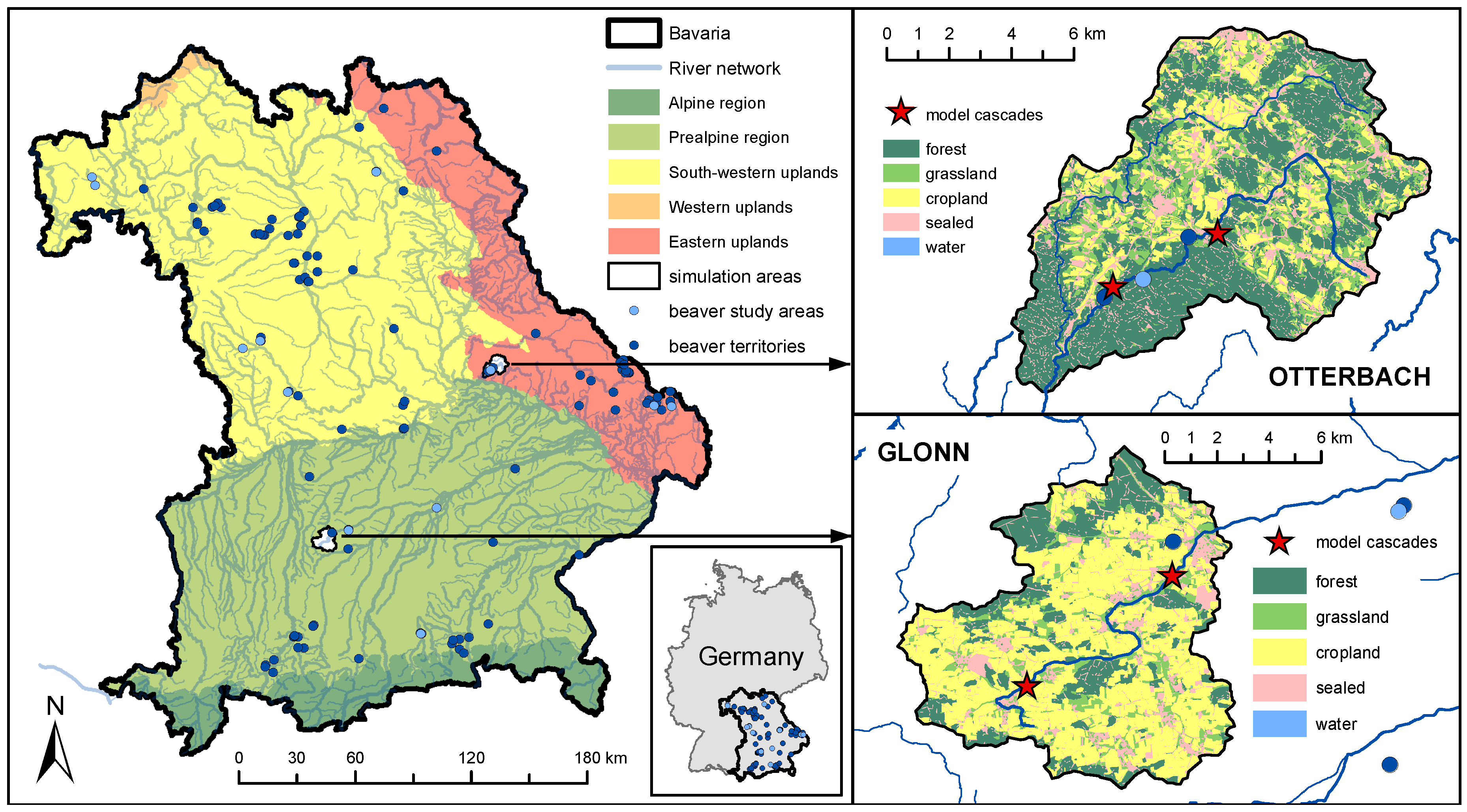
The survey of the beaver territories was performed in three steps with different levels of detail. In the first step, we conducted an online survey, which was addressed to nature conservation agencies and NGOs with local networks all over Bavaria (Bund Naturschutz, Landesbund für Vogelschutz, Landschaftspflegeverband), to gain general information about the overall distribution of beaver dams. In the second step, we selected 12 beaver study areas from the beaver territories of the survey results, in which beaver dams occurred (Figure 1). The selection criterion was to cover different geological and geomorphological regions of Bavaria, land use distributions, altitudes, catchment sizes, and slopes. The last step was a photogrammetric survey and mapping of the dam geometries and inundation areas. Aerial images were taken with a drone (octocopter: AscTec Falcon 8, Ascending Technologies GmbH, Krailling, Germany [29]; camera: Sony NEX-7, 6000 pixels × 4000 pixels, 23.4 mm × 15.6 mm CMOS-sensor, Sony Corporation, Tokyo, Japan [30]) and were analyzed to gain a three-dimensional (3D) point cloud, high-resolution orthophotos, and vector data of important structures. The accuracy of the data was usually in the range of 1 to 2 cm, and the largest deviations were about 10 cm. The selected beaver dams were additionally described including their hydraulic characteristics (i.e., freeboard, dam geometry, overflow type, and local discharge statistics).
The resulting database consists of 114 beaver dam cascades and a total number of 458 dams, which are distributed all over Bavaria and are a combination of the survey results and the 12 selected beaver study areas. The photogrammetric survey and detailed mapping was done for 51 dam locations within the selected territories.
2.1.2. Parameter Selection and Data Acquisition
The investigated parameters of the survey were defined by the requirements for the representation of beaver dams in hydraulic models, which are based on general information about the occurrence of dam cascades and the characteristics of the single dams. The parameters were classified into two stages depending on the regarded length scale and the needed level of detail.
The first stage includes parameters, which describe the surrounding of dam cascades, and are therefore decisive for the locations at which they are constructed. The total length of the cascades and the respective number of dams in the cascade were recorded in the field survey. We determined the land use distribution, the existence of copse at the river borders, and the river width and depth by a combination of the survey results, field visits, and an analysis of aerial photographs. The catchment size and the river slopes in the region of the cascades were derived from a digital elevation model with a resolution of 25 m. The discharge characteristics at the respective positions were taken from a spatial distribution of flood statistics, which was derived for Bavaria by Willems et al. [31].
The second stage contains parameters, which are necessary to describe the properties of single dams. The dam geometry (length, width, and height) was determined as part of the photogrammetric survey and resulted in 3D models of the dams. The freeboard (i.e., the upstream distance between the dam’s crest and the mean water elevation) and the state of maintenance of the dams were recorded during the field survey and by continuous measurements based on the criteria of Woo and Waddington [32].
2.2. Hydraulic Modeling of Beaver Dams
2.2.1. Modeling Concept
In view of analyzing not only the local but also the regional effects of beaver dams and the resulting computational effort, we chose the 2D hydrodynamic model HYDRO_AS-2D for modeling the investigated beaver dam scenarios. The model is developed by the Hydrotec Ingenieurgesellschaft für Wasser und Umwelt mbH and Dr. Nujić [33] and is based on the shallow water equations. The spatial discretization is realized by the finite volume method, while for the temporal discretization, the explicit Runge–Kutta method is used. This enables to model detailed structures in the floodplains, at the river channels, and for the beaver dams with unstructured meshes. The hydraulic roughness is considered by Manning’s n coefficient. The outputs of the calculated simulations are generated in 15-min time steps.
To also determine regional effects of beaver territories, it is necessary to model entire sections of the investigated rivers. To get reliable input data for the discharge curves of the flood events, the hydraulic model HYDRO_AS-2D is coupled with the physically based hydrological model WaSiM [34]. The hydrological models were calibrated and validated on the measured runoff time series of the respective gauges at the area outlets. Independent calibration and validation periods were selected and evaluated using statistical quality criteria (Nash–Sutcliffe model efficiency coefficient (NSE) and Percent Bias (PBIAS)) as well as visual analyses. The model quality lies within a range that can be classified as good according to Moriasi et al. [35].
2.2.2. Study Sites and Initial Hydraulic Models
The models were set up for the Glonn and the Otterbach catchments, which are located in Bavaria, Germany (Figure 1). The catchments have a similar size and river length but different land use distributions, valley types, topography, and geology (Table 1).
The shallow average slope and the deep brown soil with comparatively high infiltration rates and water storage capacities of the Glonn catchment result in an attenuated flow generation and concentration. In contrast, the round basin form and the high share of cropland and sealed areas shorten the response times. The Otterbach catchment shows a contrasting behavior due to its steeper slopes. Flood events are characterized by a very fast reacting peak flow and a delayed low flow which result in comparably long event durations. The river slope of the Glonn is considerably lower than the one of the Otterbach, which results in a slower flow propagation in the Glonn catchment. The river Glonn has no specific valley type, but flat and wide floodplains. Therefore, backwater due to dams may result in larger inundation areas. The dominant land use in this area is cropland and grassland, which has comparably low retention effects. The V- and U-shaped valleys of the Otterbach do not allow large flooding areas, which reduce potential retention effects. Covering the bedrock region and tertiary hills, the chosen catchments represent two of the main natural geographic regions in Bavaria.
For both investigation areas, a hydraulic model alongside the main channel without beaver dams was set up as an initial and reference model for the modeled beaver dam scenarios. The extent of the models within their respective catchments is shown in Figure 1, and Table 1 lists the most important characteristics. The elevation information is mainly based on digital elevation models with a resolution of 1 m. Additional terrestrial river surveys enable a detailed modeling of the channel course. The different land uses are represented by land use specific Strickler values (= 1/n; n: Manning’s coefficient), which are defined element-wise in the hydraulic models based on aerial photos and databases (see, e.g., in [36]). The defined hydraulic roughness doesn’t change throughout the current state scenario and the corresponding beaver dam scenarios. The ranges of the applied coefficients for the three major land use classes (see Table 1) are defined as follows; grassland: 20 ms, forest: 9–10 ms, and cropland: 9–19 ms. These ranges result from an even more detailed classification of the land uses in the models (e.g., different types of crops), which are here summarized to the three listed classes.
In general, we built these models representing a preferably close agreement with the investigated area. However, this holds not for transverse structures crossing the floodplains (e.g., road and railway embankments). These types of constructions were modified in order to reduce their impact on the development of the flood waves. The applied modification measures range from adding culverts to the crossing structures to removing them completely from the floodplain depending on their restriction classes which are defined in PAN [37]. We have not changed ditches or tributaries in the floodplains as they are part of the river system. The adaptations allow to analyze the pure effects of beaver dam cascades, which are hardly influenced or superimposed by the effects of site-specific structures, and to get a more holistic view of their contribution to flood peak attenuation. Due to the changes made, calibration on the basis of measurement data is not possible and was therefore not performed.
2.2.3. Representation of Beaver Dams in HYDRO_AS-2D
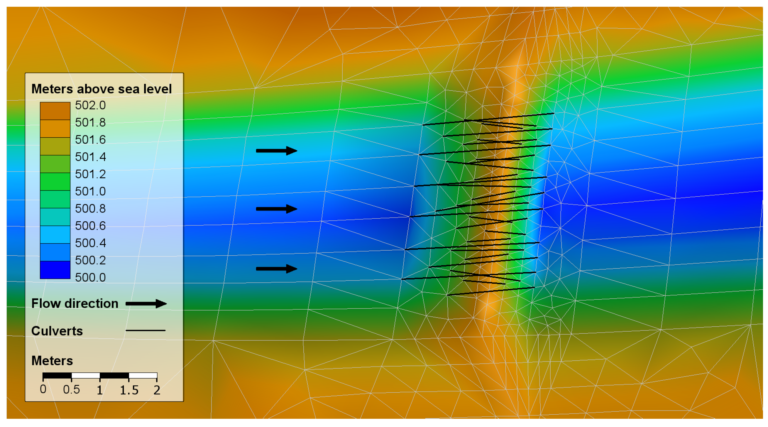
To implement the beaver territories in the hydrodynamic models, the dams of a cascade are modeled as detailed transverse structures in the course of the rivers as shown in Figure 2.
This is realized by refining the numerical mesh in the area of the dams and adapting the nodes’ elevations to match the dams’ characteristics observed in our field surveys. The hydraulic roughness of the mesh elements representing a dam was set to 8 ms for the downstream side and to 12 ms for the upstream side, which is in the range of the generally used roughness of copse and branches in hydraulic modeling [36]. The smoother surface on the upstream side accounts for the typical sludge coating attached by the beavers, which was also observed in the field. The permeability of the dams is realized by inserting round culverts (up to 70 pcs/dam) parallel to the flow direction. The locations of the culverts are homogeneously spread across the surface of the dams. To assume a reliable permeability of the dams, we calibrated the discharge capacities and number of the culverts based on the resulting freeboard at the dams, which was also one of the analyzed parameters of the field survey. This calibration process is based on the average annual discharge derived by the physically based hydrological model WaSiM. So far, dam break scenarios are not included in this study due to limited data availability in terms of stability criteria of beaver dams in combination with their vulnerability to specific flood events. The locations and characteristics (e.g., number of dams) of the modelled dam cascades are evaluated based on the developed three-stage scheme, which is described in Section 3.2.1 and builds on the results presented in Section 3.1.
2.2.4. Investigated Flood Events
Flood protection measures are usually designed to prevent damages during larger flood events, starting from return periods of 100 years. As decentralized measures and, in particular, beaver dams are assumed to have a minor impact during larger events, we considered different flood peaks. These include events with return periods of 20, 5, and 2 years, as well as an event with a smaller peak discharge corresponding to five times the annual mean discharge (5 × MD).The selected range should link the observed retention effects of recent beaver studies (e.g., [20,22]) with studies of decentralized flood mitigation measures (e.g., [27,38,39,40,41,42]).
We generated the flood events with characteristic temporal and spatial precipitation distributions by using the hydrological models in order to have comparable events with catchment dependent properties (Table 2). The precipitation distributions were scaled on two straight lines with different ratios of precipitation duration and maximum precipitation intensity. Subsequently, the generated events can be classified as advective (long precipitation duration and low intensities) and convective (short precipitation duration and high intensities) events. The differences of advective and convective events in terms of discharge volume and duration become larger with increasing peak discharges. Here, variation is larger in the Otterbach catchment compared to the Glonn catchment. In accordance with an advective precipitation event, the resulting flood events have a higher volume and longer duration compared to the ones based on convective rainfall events.
The peak discharges of the generated flood events match the statistical data of the gauges (Glonn: Odelzhausen, Otterbach: Hammermühle) at the outlet of the hydrological models for the respective return periods. The values in Table 2 were taken from the hydraulic models, which were used for the scenario implementation. They differ from the hydrological models in terms of a more precise routing methodology, which explains the mismatch of the advective and convective peak discharges. A stationary warm up period of about 20 h corresponding to the mean annual discharge is added prior to the event to guarantee that the river channel is realistically filled when the event starts.
2.2.5. Evaluation of Hydraulic Model Results
The peak discharge attenuation and translation are among the most common parameters to estimate the effectiveness of natural retention measures. To consider the local and regional impacts of the dam scenarios, the discharge curves of the beaver dam scenarios and the respective current state models are analyzed downstream of the beaver dam cascades at reasonable cross sections as well as at the model outlet. The peak attenuation and translation at these locations are calculated using Equations (1) and (2). Here, refers to the maximum peak discharge of the analyzed discharge curve, while is the time, at which occurs.
A positive attenuation refers to a smaller peak discharge in the beaver scenarios compared to the respective current state scenarios. A positive translation means a delayed peak discharge in the beaver scenario.
Furthermore, the impact of the beaver dam cascades on the maximum water levels and flooded areas is determined. For the comparison of spatial results (e.g., water depths), the quantities based on the unstructured calculation meshes, which are different in the scenarios due to the added dams, are interpolated to a regular grid (resolution: 0.4 m). Based on this grid, the beaver-influenced area is evaluated considering the differences of the maximum reached water levels. Also, the differences of the water levels during the stationary warmup period (mean annual discharge at the gauge), were considered. Here, a threshold of 0.03 m was set to determine the influenced raster cells. The water volume (), which is additionally activated by the beaver dam cascades, is determined for each cascade-flood event combination based on the influenced area. It is calculated following Equation (3). Here, corresponds to the used water volume in the influenced area during the maximum reached water levels. refers to the water volume, which is already used at the very beginning of the flood event during the stationary warmup period. The same holds for the current state.
The volume of the flood event between the end of the warmup period and the peak discharge is relevant for the efficiency of flood retention measures. It is called in the following.
3. Results
3.1. Analysis and Characterization of Beaver Territories
Beavers influence the runoff characteristics by the construction of dams and a subsequent impounding of the rivers. However, the majority of beaver territories are located in ponds, lakes, rivers, or streams that already meet beaver habitat requirements, and therefore no beaver dam construction activity is observed. Therefore, the analysis was focused on territories with dams in order to define characteristics in the surrounding of rivers, which are decisive for the construction of dam cascades.
3.1.1. Characteristics of Dam Cascades
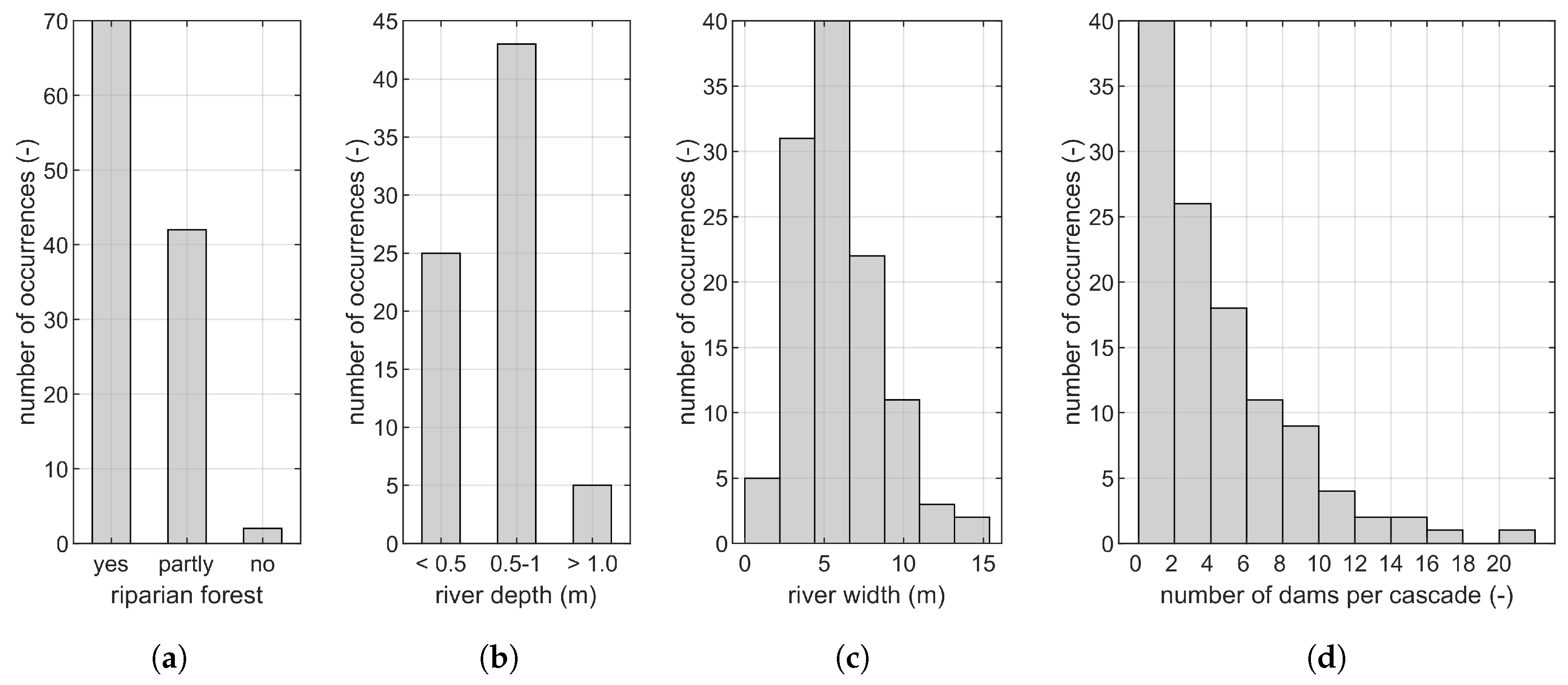
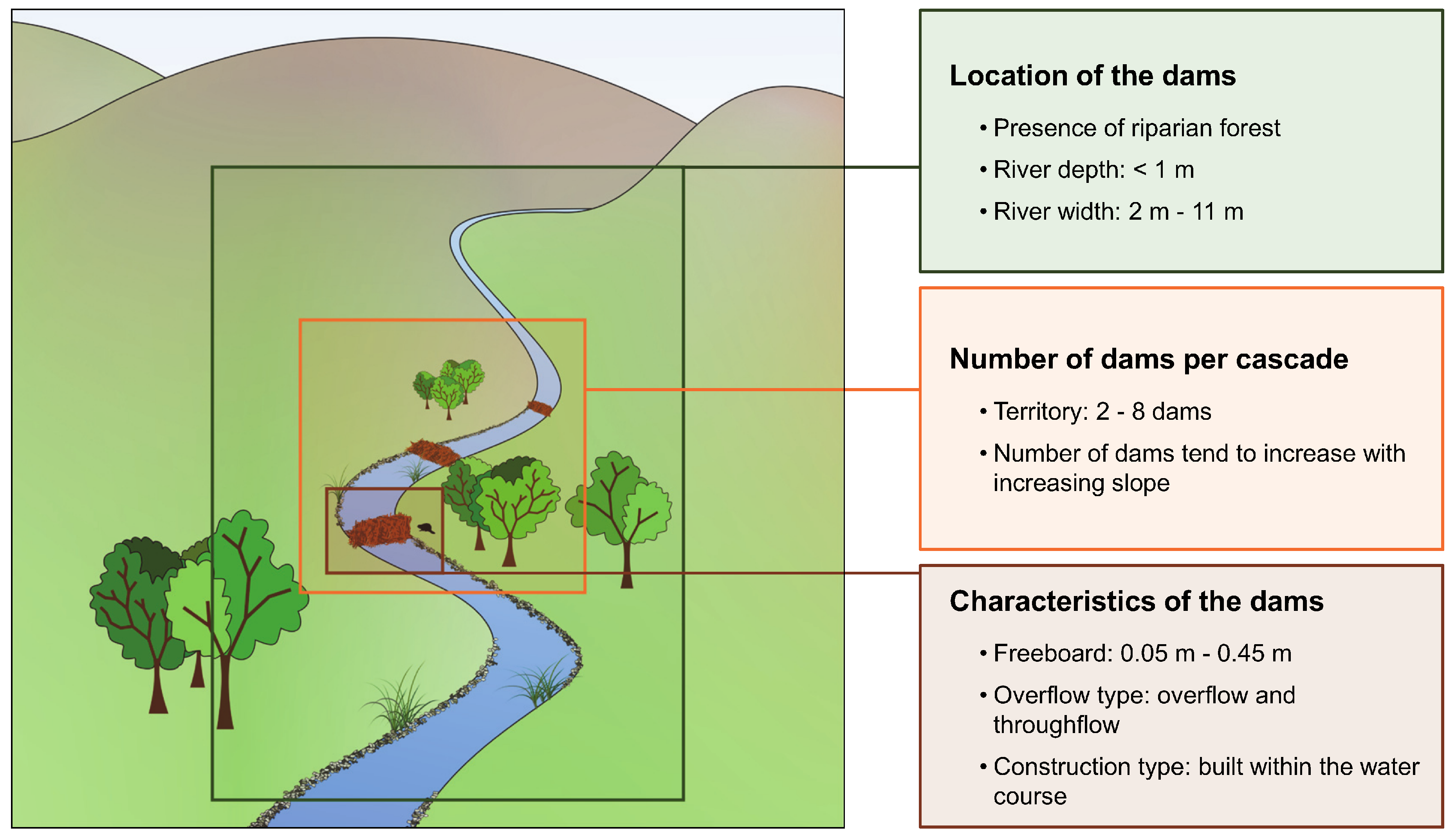
The locations of the beaver dam cascades are affected by the present riparian forest, the river depth, and the river width. Figure 3a shows that dams are most likely constructed if forest occurs at the river borders. Only 2% of the dam cascades were located at river sections without any riparian forest, whereas 60% were within uniformly forested areas.
Partly forested areas include single trees, but no continuous dense forest. Riparian forest in the surrounding of beaver dams usually comprise willows and poplars, which also serve as food for beavers. Beaver dam cascades were particularly observed at river sections with shallow water depths below 1.0 m (Figure 3b). Approximately 59% of the cascades were located in rivers with depths of approximately 0.5 to 1 m, which is therefore the most likely range of water depths for the occurrence of beaver dams. The river width, which occurs at full channel flow, is approximated by measurements at several unaffected positions near the beaver dam cascade. The investigated dams were located in rivers with a width of up to 15.4 m (Figure 3c). The lower and upper quartiles of the observed widths are 3.8 m and 7.6 m, respectively, whereas 90% of the observed dams lie within a range of 2 to 11 m.
The investigated dam cascades showed a large probability toward low numbers of dams per cascade (Figure 3d). Approximately 34% of the territories consisted of only one dam, whereby the median of the number of dams per cascade is 3. If considering only territories with cascades consisting of more than one dam, the lower and upper quartiles are three and eight dams per cascade, respectively.
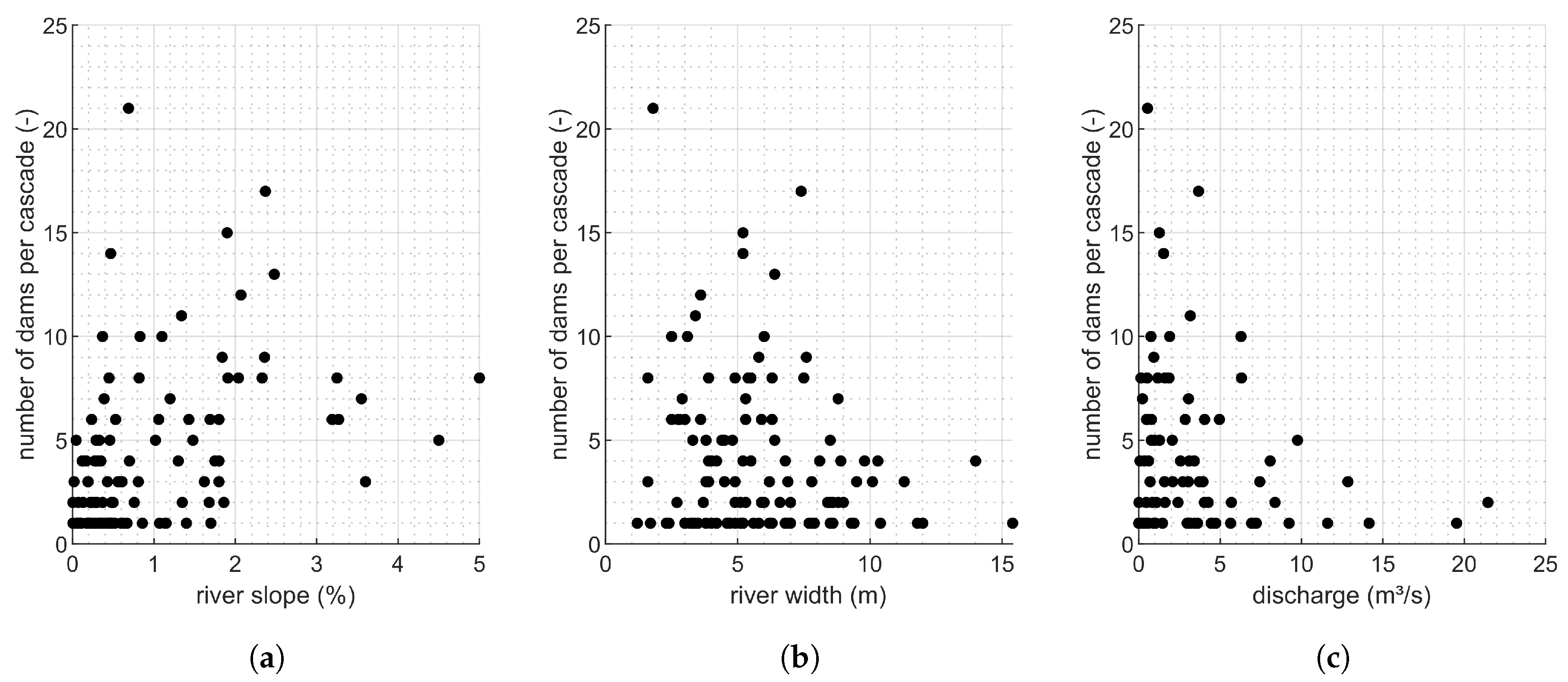
To explain the different numbers of dams per cascade, we examined their dependencies on the river slope, the river width, and the peak discharge for a return period of two years (Figure 4). A tendency of an increasing number of dams with an increasing river slope was observed (Figure 4a, ; with r: Pearson correlation, p: p-value). A clear correlation between river width and the number of dams per cascade could not be established. Nevertheless, the maximum number of dams per cascade, which has been observed for a specific river width, decreases with increasing widths. Figure 4c shows that most dam cascades are located in rivers with relatively low discharges. Additionally, a decrease of the maximum observed number of dams per cascade with an increase of the flow rate can be observed. Generally, no strong dependency or correlation could be found to explain or predict the specific number of dams per cascade.
3.1.2. Characteristics of Beaver Dams
In total, 51 dams were analyzed in terms of freeboard, dam height, dam width, overflow type, and construction type based on photogrammetric surveys and detailed mapping (Figure 5). Approximately two-thirds of these dams are located in regions affected by the management of local water authorities or farmers (i.e., dams are removed or beavers are resettled from time to time). The boxplot in Figure 5a shows the distribution of the observed freeboards. The median of 0.07 m and the upper quartile of 0.12 m show that most of the freeboards lie in the lower part of the observed range between 0.00 m and 0.45 m. Dam heights of up to 1.70 m were observed. The dam heights are measured from the bottom of the river channel to the top of the dam’s crest. As shown in Figure 5b, the observed heights have a lower quartile of 0.49 m and an upper quartile of 0.81 m. The dams’ widths show a large bandwidth between 1.5 m and 75.0 m (see Figure 5c). Nevertheless, 50% of the captured widths are within the range 5 to 19 m. The width of a dam also depends on the construction type, i.e., dams reaching in the meadows result, on average, in the largest widths, while dams constructed completely in the river show the smallest widths.
The overflow types of the analyzed dams were clustered in three categories: overflow (primary stage), gapflow (secondary stage), and marked gapflow (tertiary stage). The respective shares of observed occurrences are 12%, 39%, and 49% (Figure 5d). All of these overflow types are combined with a varying discharge component through the dam itself (throughflow). The present overflow type is often linked to the dam’s state of maintenance by the beaver. Dams of the primary state are characterized by ongoing maintenance. Their construction material often consists of recently gnawed branches, and the upstream face of the dams has a coating out of sludge, which leads to a lower permeability of the dam. The secondary stage includes dams consisting of both old and fresh branches, and the dam’s crest can be overgrown. As the dams of this stage show a lower maintenance level by the beaver, small breakages can occur. In contrast, dams of the tertiary state consist of old branches and are not maintained by the beaver anymore. The crest of the dams is often overgrown, and the sludge coating is nonexistent. The dams show a high permeability and have breakages.
Figure 5e shows the distribution of the construction type of the considered dams. Here, 47% of the dams lie completely within the river, which is also the most likely observed construction type. Approximately 20% of the dams are higher than the river banks, whereas 33% reach into the meadows.
3.2. Implementation of Dam Cascades in the Hydraulic Models
3.2.1. Scheme for the Derivation of Potential Beaver Dam Locations
We developed a three-stage scheme (Figure 6) to create reasonable beaver dam scenarios in the hydrodynamic models. Each of the three stages represents a step of creating the dam cascades by taking the decisive parameters into consideration. In doing so, the parameters resulting from our filed surveys and questionnaires, which are described in Section 3.1 (e.g., river depth, river width, freeboard, and overflow type), were analyzed with respect to their frequency distributions.
The first stage defines the parameters which have to be fulfilled for the occurrences of beaver dams alongside the investigated river. According to the results of the analyzed territories, the presence of riparian forest, a river depth smaller than 1 m, and a river width ranging from 2 to 11 m were defined as thresholds for locating the dams. After defining an appropriate location, the number of dams in the scenario cascade is set in consideration of the channel and the floodplain slope (second stage). Based on the field survey, the number of implemented dams is set between three and eight with a higher number for increased slopes. The third stage deals with the characteristics of the dams. We decided to model dams within the river courses, as it was the construction type which was most frequently observed. The dam’s freeboard, which also depends on the permeability of the dam, is chosen within the measured values between 0.00 m and 0.45 m. As the dam scenarios are related to flood mitigation, we chose a combined throughflow–overflow construction type for the scenarios. This type was only observed for 12% of the investigated dams but results in the highest available retention volumes, which are necessary for affecting flood events.
3.2.2. Definition of Beaver Dam Scenarios
A total of 12 beaver dam scenarios were investigated in separate hydraulic models to determine their impacts on eight different flood events. Two beaver dam cascades were developed for both hydraulic study sites (Otterbach and Glonn) following the three-stage scheme described in Section 3.2.1. To analyze also the location-dependent effects of a cascade within the investigated area, it was an additional objective to find appropriate locations in the upper and lower parts of the catchment. The exact locations of the cascades are represented in Figure 1. Each of the two cascades (C, upstream cascade; C, downstream cascade) was separately implemented in the initial hydraulic model of the respective investigation areas. In addition, a third hydraulic model considers the occurrence of both dam cascades at the same time (C). The distances between the dams within a cascade are related to the beginning of the backwater effect of the downstream-situated dam, which was estimated by intersecting the dam crest height with the upstream river channel and the floodplains. The resulting distances are within the range of the observed distances. They are listed among other characteristics of the respective cascades in Table 3.
Table 3 lists the characteristics of the four developed beaver dam cascades. C in the Glonn catchment consists of three dams and is located in a river section with a channel slope of 0.5‰ and wide floodplains representing the flattest dam cascade position. In contrast, C, in the Otterbach catchment, is situated in a narrow V-shaped valley section and is composed of seven dams. It is the steepest cascade with a channel slope of 41.1‰. Both C-cascades are located in a river section with comparable channel slopes (Glonn: 4.1‰, Otterbach: 5.2‰) and consist of three dams.
Considering the direct relation between the freeboard and the available retention volume, we decided to model all beaver dam cascades as fully maintained dams (low permeability, small freeboard between 0.05 m and 0.15 m) and rarely maintained dams (high permeability, large freeboard between 0.35 m and 0.45 m). The scenarios modeled with high permeability are indicated by the index h, whereas the ones modeled with low permeabilities are labeled with the index l.
3.3. Impact on the Investigated Flood Events
3.3.1. Flood Peak Attenuation and Translation
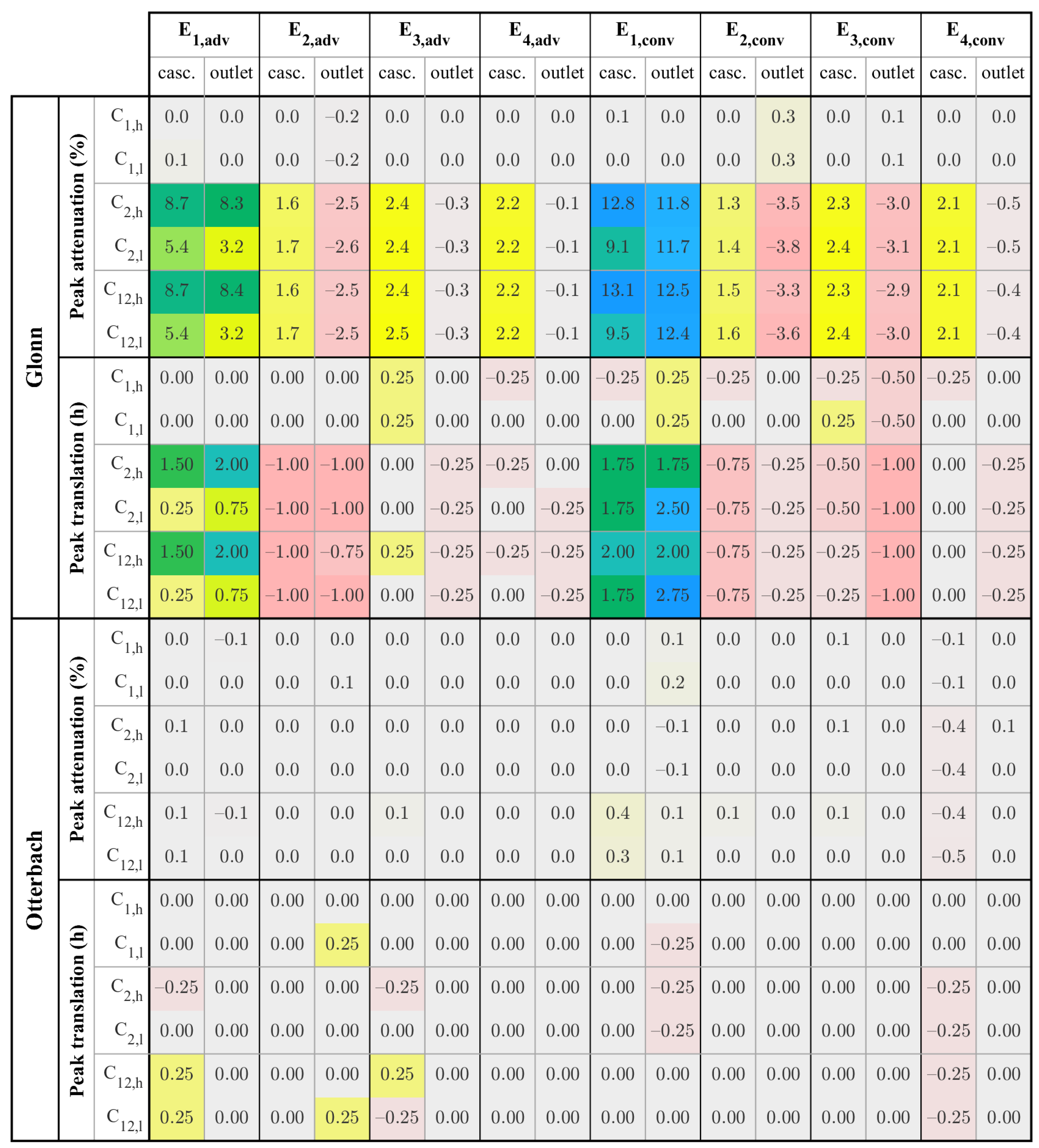
A considerable peak discharge attenuation (>0.5%) and translation (>0.5 h) was only observed as an effect of cascade C at the Glonn and is particularly visible for small flood events (Figure 7). For most events, the peak discharges of the dam scenarios show a local reduction at the cascade, while the effect is slightly lower or even negative at the model outlet. The differences of the defined freeboards have an impact only during the E events. The effects of the other cascade on the hydrograph as well as the effects of both cascades at the Otterbach are negligible. The characteristics of the investigated flood events (E to E, each adv. and conv.) at the dam cascade locations are listed in Table 4 in addition to the characteristics at the outlet (Table 2).
The maximum observed peak attenuation of 13.1% occurred during event E for the C scenario at the Glonn. Generally, all scenarios considering cascade C at the Glonn reached distinctly larger attenuations during the two small flood events E and E compared to the other flood events with higher discharge peaks and flood volumes. The differences in peak reduction of event E and its corresponding advective event E may also be explained by the higher peak discharge (+11%) and (+48%) of the advective event (Table 4). However, the different flood volumes of advective and convective events have no distinct impact on the retention effect for the other events. Another exception to the observed dependency of the peak attenuation from is the low peak reductions during the E events. The reason for this effect is the event-dependent impact of a drainage ditch on the floodplain, which is running parallel to the river channel and enters the river approximately 225 m downstream of cascade C. The inundations in the floodplains, which are caused by cascade C, activate the flow in the drainage ditch during the smaller flood events and result in complex superposition effects depending on the respective timing.
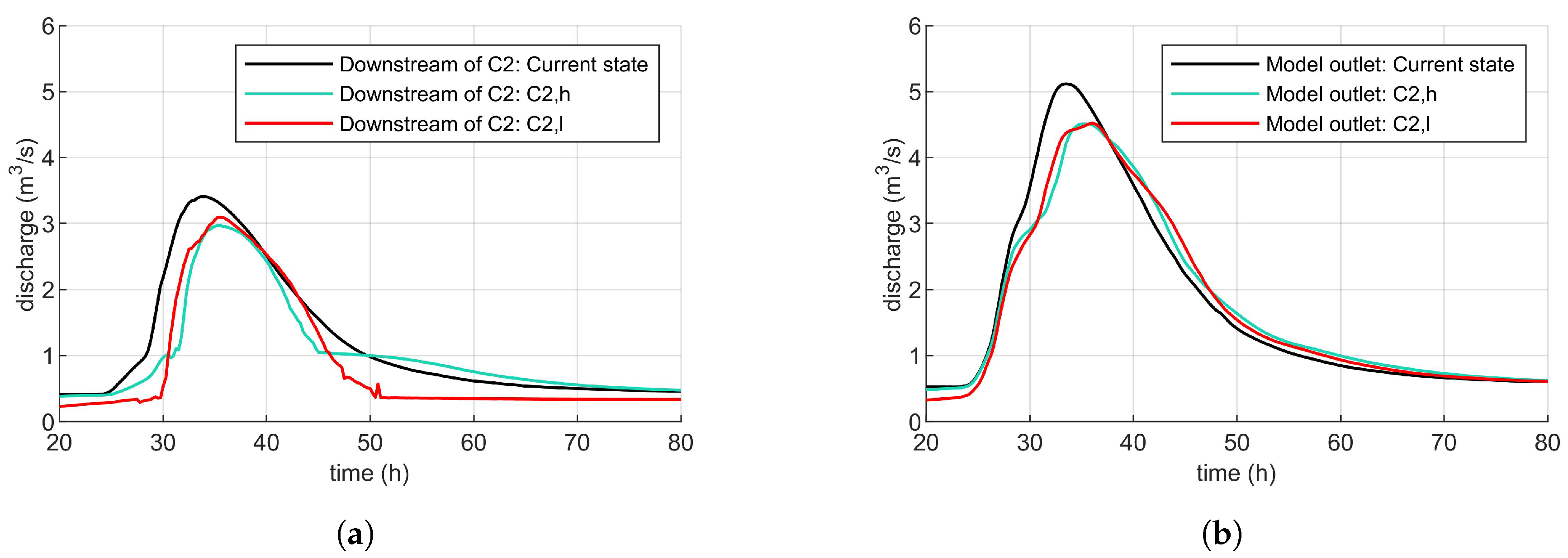
Figure 8 displays the discharge curves of the current state scenario and the scenarios C and C downstream the cascade C (Figure 8a) and at the model outlet (Figure 8b) for event E. Here, the different shapes of the discharge curves of the dam scenarios account for the different permeability parameterizations. At the cascade location, the curve of scenario C raises slower compared to C, as the cascade C has an increased available retention volume due to the larger freeboard. The effect of the permeability can also be observed in the descending part of the curves, where more water is released in scenario C compared to the low-permeability parameterization C. In contrast, the differences between the two shown freeboard scenarios are almost negligible at the model outlet (Figure 8b).
The comparison of the local and the regional effects of dam cascade C at the Glonn mostly shows considerable differences of the peak attenuations (Figure 7). The changes arise due to the superposition of the flood wave with the inflow from a major tributary downstream of the cascade C, which increases the catchment area by 22%. The superposition effect is sensitive to the timing of the peak discharge and thus depends on the event characteristics. It usually results in a decreasing or even negative peak attenuation, but can also cause an increased effect (e.g., cascades C and C during the event E).
The translations show, just as the attenuations, only considerable effects for cascade C at the Glonn. The largest translations with up to 2.5 h are reached during the two small flood events E and E. In this case, the retention effects of the dams cause a decreased and a delayed peak discharge. The translations of these two flood events show a dependency on the definition of the available freebord, which has also been observed for the respective attenuations. Higher freeboards tend to result in larger delays of the peak discharge. The translations at the model outlet are also influenced by the confluence with the already mentioned major tributary. The results of all flood events demonstrate that there is no general dependency between the attenuation and the translation of the discharge curves. Even if there is a positive attenuation at the cascade location, the peak discharge is often reached prematurely in comparison to the current state model. This effect arises due to the impact of the previously mentioned drainage ditch on the floodplain next to cascade C at the Glonn. The additionally or earlier activated flow path in the ditch during the dam scenarios causes the observed earlier peaks in combination with the positive attenuations. In general, the resulting translations of the peak discharges tend to decrease with increasing flood events.
The results of the Otterbach catchment show almost no local or regional impacts on the discharge curves of the investigated flood events.
3.3.2. Impact of Topographical Characteristics on the Effects of Beaver Dam Cascades
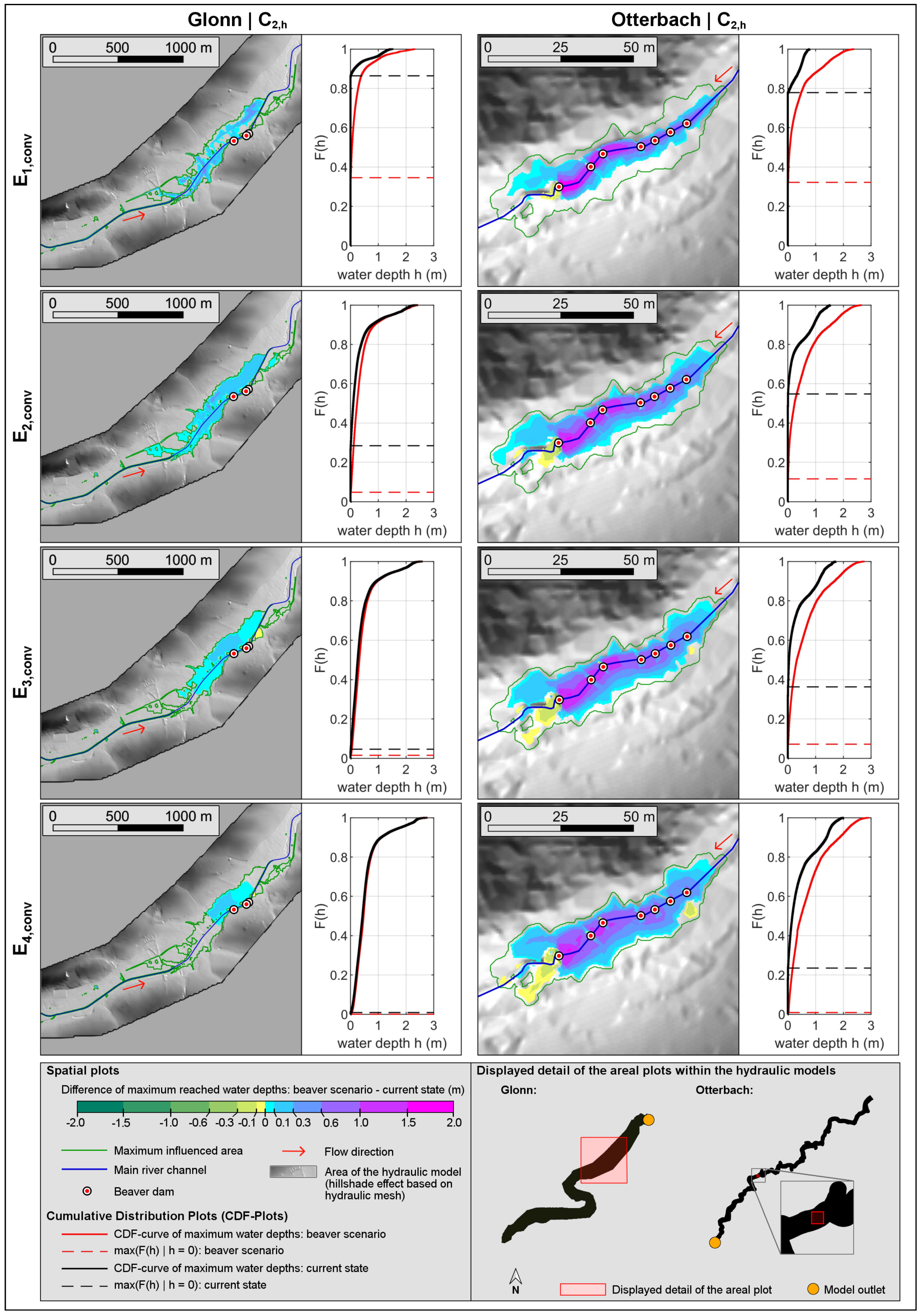
The combination of evaluating the discharge curves and spatial water level analysis showed that the topographical characteristics influence the impacts of the beaver dam cascades on flood events. Figure 9 visualizes the areas influenced by the beaver dam cascades C in the Glonn and Otterbach catchment for the convective flood events E–E. The green line in the spatial plots refers to the area that is maximal influenced by all scenarios containing cascade C during any flood event. The colored areas indicate the differences in the maximal reached water levels between the C scenario and the current state. Additionally, the cumulative distribution functions (CDF) of the corresponding maximal reached water depths within the maximal influenced area are shown. The red line corresponds to the beaver dam scenario while the black line refers to the current state. Consequently, the colored water level differences in the spatial plots map the gaps between the two respective CDF curves. The horizontal dashed lines in the CDF plots indicate the share of dry raster cells ( m) within the maximal influenced area.
For both catchments, the maximal flooded area within the maximal influenced area increases with raising peak discharges, which is indicated by the lower number of dry raster cells represented by the horizontal dashed lines in the CDF plots. Concurrently, the difference between the flooded area of the cascade scenarios and the current state decreases. The differences in the maximal reached water levels show a catchment dependent behavior caused by dissimilar topographic characteristics like the slopes of the river channel, the floodplains, and the valley type (see Section 3.2.2).
The cascade at the Otterbach results in a clearly smaller maximal influenced area compared to the cascade at the Glonn due to the steep and narrow valley section (Otterbach: 2.2 × 10 m, Glonn: 246.2 × 10 m). In the case of the Otterbach catchment, the shapes of the two CDF curves, which describe the cumulative distribution of the maximum reached water depths for each scenario, differ considerably throughout all events. This results in relatively large remarkably influenced areas (displayed by the colored raster plots) compared to the maximum influenced area (displayed by the green line) over all events. On the one hand, the steeper gradient of the lower tails of the red CDF curves indicate that in the dam scenario more raster cells are affected by small flow depths. On the other hand, the lower gradient of the upper tail states a distinct increase of the maximum occurring water depths by the dams. In contrast to the Otterbach, the impact of the dams on the maximum reached water depths at the Glonn is more related to the considered flood events. The CDF curves in the top left corner show that during the E event both the shallow inundated areas and the larger occurring flow depths are increased by the beaver dams. Here, the share of dry cells (horizontal lines) demonstrates that the flooded area in the dam scenario increases by 96.4 × 10 m or 359%, which is the largest relative rise throughout all modeled scenarios. For the events E – E, the influenced areas displayed by the raster plots decrease with increasing discharge peaks. This can also be seen by the approaching CDF curves of the two scenarios. For those events (E – E) the maximum occurring water depths are hardly increased by the dams.
The simulations also show that the water depth is slightly decreased by the dams in some small areas downstream of the cascades. Directly at the locations of the beaver dams, a larger decrease of the water depths occurs (up to 2 m). This results from the implementation of the dams which implies a higher elevated computation mesh resulting in lower flow depths compared to the current state. In contrast, the absolute water levels are often increased.
Beside the two cascade scenarios in Figure 9, the results of all cascade scenarios show the tendency of a decrease of the additionally flooded area with increasing flood peaks. The same trend was observed for the differences in the maximum reached water levels. Consequently, also tends to decrease with increasing peak discharges. There are just a few exceptions in the case of the C cascades in combination with the very small E events. In these cases, the discharges are too small to cause large flooding resulting from the dams. Thus, the can even get negative as there is already a considerable backwater in the river channel for the dam scenario during the warm-up period. Therefore, the increase of the used water volume during a small flood event with small inundation areas in the beaver dam scenario can be slightly lower compared to the current state (see also definition of in Section 2.2.5).
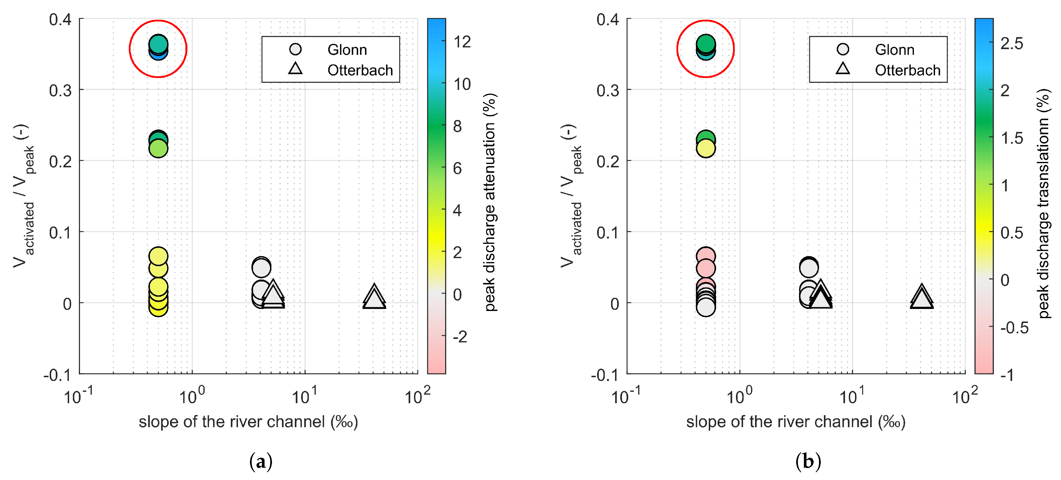
Figure 10 shows the connection between the channel slope and the proportion of (additionally activated water volume in the model by the beaver dams) divided by (flood volume between the end of the warm-up period and the peak discharge) for each dam scenario in both catchments. The is set in relation to as it is relevant to activate preferably large additional retention volumes in order to affect the peak discharge of a flood event. The largest proportions resulted from cascade C at the Glonn, which is located on a river section with a low channel slope in combination with wide floodplains. In contrast, the resulting from the steeper dam cascades at the Otterbach are negligible small compared to . The peak discharge attenuations at the dam cascades (Figure 7) are displayed as a third parameter in Figure 10a. It shows that a relatively large with respect to results in the highest peak attenuations. In some cases, location-specific small-scale effects, like the influences of the drainage ditch in the Glonn catchment, can influence the results. An example for this can be seen in the top left corner of the plot. The four uppermost scatter points indicated by the red circle represent the scenarios including cascade C at the Glonn during the E event. Here, the scenarios with a low freeboard have a higher compared to the scenarios with a high freeboard. However, the scenarios with a low freeboard result in lower peak attenuation, due to the impacts of the drainage ditch. The relatively small resulting from cascade C at the Glonn and both cascades of the Otterbach in combination with a moderate to high channel slope result in negligible attenuations. Figure 10b displays the results with the translations included in Figure 7 as the third parameter. In general, the translations show comparable tendencies to the attenuations. Here, a high ratio of divided by also results in the largest impacts on the translation. In case of the scenarios containing cascade C at the Glonn, the impact of the cascade shows also the small-scale effects of the drainage ditch resulting in negative translations. In accordance with the attenuations, the other three cascades have no remarkable impact on the translations.
4. Discussion
4.1. Survey and Analysis of Beaver Territories
Based on the results of the questionnaire (114 beaver territories, 458 beaver dams) and the detailed field survey (12 beaver territories, 51 beaver dams), an overview of the dam building activities of beavers in the streams of Bavaria was obtained. Our findings revealed that 90% of the beaver dams were observed in small streams with a width ranging from 2 to 11 m and 59% of the streams were in a depth range of 0.5 to 1 m. These results coincide with observations from other studies, which showed water depths of less than one meter and variable widths ranging between 0.5 and 46 m [16,18,43,44,45]. In Bavaria, beavers show similar activity patterns as observed in other regions. Our findings, that about one-third of the cascades consist of only one dam and 50% of the larger cascades include three to eight dams, are comparable to the data compiled by Danilov and Fyodorov [44] (2–9 dams) and Nyssen et al. [22] (1–6 dams). Although 50% of the investigated Bavarian beaver dams have a height of 0.5 to 0.8 m, some of them reached heights of up to 1.7 m. Even though previous studies on beaver dams report dam heights between 0.3 and 5 m [45], the bulk of published data suggests that their height tends to be less than 1.5 m [22,46]. A general range of the dam widths between 1.5 and 75 m was obtained, while 50% of the widths were between 5 and 19 m. Our observations coincide with the numbers obtained by Butler and Malanson [47] indicating that beaver dams typically have a length of 15–70 m.
In general, many beaver territories in Bavaria are influenced by anthropogenic impacts. Approximately two-thirds of the surveyed dams were managed by farmers or local water authorities, which for instance remove dams or resettle beavers. Therefore, the data we collected about territories or dam characteristics can be biased by this effect. Nevertheless, the results of the survey and the investigations of the cascades and dams match observations of the dam building behavior of the Eurasian beaver in Sweden, where the dams are not intensively managed [16].
4.2. Development of Hydraulic Beaver Dam Scenarios
Based on the surveys and the detailed investigations of the beaver territories, we developed a three-stage model, with which reasonable dam cascades in the investigated catchments can be predicted for the hydraulic modeling. The output of this prediction model is mainly based on the statistical occurrences of the observed data. Additionally, a cross-correlation analysis of different parameters has been conducted to acquire near-natural dam cascades. Therefore, the characteristics of the developed beaver dam scenarios match the observed data. No strong correlation between the number of dams per cascade and site-specific characteristics could be determined, but there was a trend ( ), which indicates a higher number of dams per cascade with an increasing river slope. To take these uncertainties into consideration, we modeled four cascades with three to seven dams per cascade, which fit the number among the observed territories. Our decision to restrict the modeled construction type to dams, which are completely within the watercourse, was based on the most probable occurrence of this type and is meaningful with regard to the modeling and computational effort. Nevertheless, this construction type may not be the one resulting in the maximum retention effects during flood events. Thus, future studies about modeling beaver dams should consider the contribution of the construction type on flood mitigation effects. In general, the application of the developed three-stage model ensures the consistency of the generation and the modeling of beaver dam cascades. It increases the comparability of the different investigated scenarios and enables conclusions of site-specific hydromorphological and topographical properties and their impacts on flood events. Different methods for the prediction of beaver habitats and dam building activities of the castor canadensis and the castor fiber have been developed for North America, Sweden, and the lowlands of Belgium and the Netherlands in recent decades [16,17,18]. Most of them include the same parameters to predict suitable beaver territories as we considered in our study (e.g., stream slope, river width, river depth, and riparian vegetative conditions). Nevertheless, the different regional conditions as well as potential species-specific behaviors decrease the transferability of these models to our study areas. We therefore consider our results and the developed prediction model as a valuable contribution to the existing database.
4.3. Model Approach
We coupled the physically based hydrological model WaSiM with the 2D hydraulic model HYDRO_AS-2D to determine the impact of beaver dam cascades on flood events. The modifications of transverse structures without runoff regulation purposes allowed to analyze the pure effects of potential beaver dam cascades, but excluded a calibration of the hydraulic model on measured data. Nevertheless, comparability of the scenarios is guaranteed by the consistency of the models in terms of model setup and roughness parametrization. The investigated flood events, which were generated with the hydrological model, are design events of specific return periods, but correspond to the typical event characteristics of the study areas. The beaver dams are included in the hydrodynamic model as transverse structures with multiple openings. This representation can be considered to be adequate for the chosen throughflow-overflow dam type. The scope of this study was to determine the impact of beaver dam cascades on a local (downstream of the cascades) and a regional scale (at the gauge). 3D hydraulic models could represent the hydraulic conditions directly next to the dams in a more realistic way compared to 2D models. However, the computational effort of 3D models would be too large for a regional analysis, whereas the scale requirements are covered by the capabilities of the chosen 2D model HYDRO_AS-2D. The model as well as the combined application with WaSiM has already been used successfully for the analysis of natural and decentralized flood retention measures [25,27,41,48,49], and thus can be classified as proven approach for the investigation of measures related to the river channel or the floodplains during flood events.
The uncertainties in the hydrodynamic models are hard to estimate, as the scenarios are based on hypothetical beaver dam cascades and thus cannot be compared to measurements. However, the overall results show reliable behavior of the dam cascades indicating almost no effects for large flood events and some small effects during discharges with small return periods. Furthermore, HYDRO_AS-2D was originally developed for modeling dam break scenarios [50], which implies that the internal algorithms can also cope with challenging flow situations, which might also occur in the areas of the beaver dams.
Due to the lack of data regarding the stability of beaver dam cascades during flood events, dam break scenarios were not modeled in this study. Consequently, the modeled cascades represent best case scenarios without considering the risk of a single dam break or a series of dam breaks in a cascade. Further studies should therefore include an evaluation and discussion of comprehensive effects of beavers on flood events. These could for example include the increased risk of log jams due to the material of broken or damaged beaver dams or the influence of beaver digging activities on existing technical flood protection measures like dikes.
4.4. Impact of the Investigated Beaver Dam Cascades on Flood Events
The applied approach, which combines six different beaver dam cascades with eight flood events in two catchments, allowed a profound analysis of the contribution of beaver dams to flood mitigation. The evaluation of the hydraulic simulations showed that the impact of the dam cascades on flood events depends on the hydromorphological and topographical characteristics of the study site as well as on the event itself. The observation that dam cascades only affect small flood events, if the cascade is located in a river section with a low channel slope and flat floodplains highlights the interaction of the influencing factors. This matches the findings of Westbrook et al. [24] stating that beaver dams are only able to extensively increase both the hydraulic head and the flooded areas in flat valleys with broad floodplains.
The noticeable attenuation and translation of small peak discharges with up to 13.1% and 2.75 h support the findings from previous studies [20,22]. Nevertheless, the retention effects resulting from the modeled beaver dam cascades during larger events are only small or even negligible in both catchments and are therefore not relevant in terms of flood mitigation measures. It is not possible to define an exact discharge level or return period at which the flood peak reduction by beaver dams becomes ineffective as local topographical characteristics have a large influence. The impact of the available storage volume influenced by the dam’s permeability is only visible for small peak discharges in case of cascade C at the Glonn (see Figure 8a). The resulting shape of the raising parts of the discharge curves during these events shows the typical behavior of small retention basins. However, this effect is by far not as pronounced as for anthropogenic retention basins, because the available storage capacity of beaver dams is by orders of magnitude lower [26,27,28]. No relevant influences of the dams’ permeabilities could be observed during larger flood events. The simulations also showed that the flooded areas increase by up to 359% due to the occurrence of beaver dams. These additional inundation areas could cause some human–wildlife conflict as it is also assumed by Swinnen et al. [18].
Additionally, the cascade C in the Glonn catchment showed how catchment specific small-scale effects can influence the impact of the beaver dam cascades. On the one hand, artificial constructions like drainage ditches can affect the impacts of the cascade. On the other hand, the superposition effects with flood waves of tributaries can also have an event-dependent positive or negative effect on the reached peak attenuation or translation. Therefore, the impacts of dam cascades on small flood events are hard to predict without the help of appropriate models and emphasize the importance of the evaluation of regional effects. It can be assumed from the results that the transverse structures, which were modified during the model setup, would have an even greater influence on the discharge behavior. Although they were not constructed to regulate runoff, they would mask the effect of the beaver dams and thus prevent their quantification. In contrast, the ditches and tributaries in the floodplains have a discharge function and therefore cannot be removed without changing the natural or deliberately anthropogenically altered discharge behaviour. As a consequence, the transferability of the observed numerical values to other areas is only possible to a limited extent.
Although the investigated dam cascades cannot remarkably contribute to natural flood mitigation measures, the hydraulic characteristics (e.g., flow depths, inundation areas, and occurrence of beaver ponds) of the water courses are changed. Therefore, the observed effects due to the presence of beaver territories is in accordance with the positive impacts on the ecological diversity of the riparian habitats and the water quality stated in recent studies (see, e.g., in [19,20,22,23,24]).
5. Conclusions
The evaluation of 114 beaver dam cascades and the detailed survey of 51 dams enabled the development of a three-stage prediction model for developing likely beaver dam cascade locations and configurations. Based on this prediction model, scenarios were developed to represent different potential beaver dam cascades in 2D hydraulic models using a consistent methodology. By modeling 12 cascade scenarios in total in two catchments during eight different flood events, a well-founded analysis of the hydraulic impacts of beaver dams on flood events is enabled.
Our hypothesis that beaver dam cascades result only for small flood events in remarkable retention effects is proven by the modeling results. As the research demonstrates, the modeled dam cascades have no considerable impact on the peak discharge attenuation for flood events with return periods of 2 or more years in terms of flood mitigation measures. The importance of the site characteristics is demonstrated by the observed differences among the cascades. The three cascades, which were located in a V- or U-shaped valley sections with channel slopes of at least 4.1 resulted in remarkably low peak discharge attenuation and translation. In contrast, the cascade with wide floodplains and a flat river slope of 0.5‰ caused considerable peak attenuation (up to 13.1%) and translation (up to 2.75 h) for smaller peak discharges. For larger flood events (return period ≥ 2 years), the impact on the peak attenuation is notably lower at the cascade (about 2%) and negligible at the basin outlet (about 0%).
Scenarios resulting in a high additionally activated volume compared to the respective flood volume had the largest impact on the peak discharge. The relative magnitude of the activated volume itself depends strongly on local topographical characteristics like the channel and floodplain slope as well as the shape of the valley. Consequently, the impact of beaver dam cascades on flood events depends strongly on the local characteristics of the catchment and the magnitude of the flood event.
We suggest that apart from looking for the effects of dams built within the river channel, future research should also analyze the impact of other construction types (e.g., dams reaching into the meadows) as well as the effect of dam breaks. We conclude from our results that beaver dam cascades only result in a retention effect if the local topographical characteristics support the activation of a sufficiently large additional retention volume compared to the event volume. In consequence, peak reductions may occur for beaver dam cascades at river sections with low channel and floodplain slopes and wide floodplains during small events, but beaver dams still cannot be considered as flood mitigation measures. The results of the study are relevant for the assessment of beaver dams as part of nature-based solutions for flood protection decision-making.
Author Contributions
Conceptualization, M.N., S.T., S.S., V.Z., and W.R.; methodology, M.N., S.T., S.S., V.Z., and W.R.; software, M.N. and S.T.; formal analysis, M.N. and S.T.; investigation, M.N., S.T., S.S. and V.Z.; data curation, M.N., S.T., S.S., and V.Z.; writing—original draft preparation, M.N. and S.T.; writing—review and editing, M.N., S.T., S.S., V.Z., and W.R.; visualization, M.N. and S.T.; project administration, S.T., V.Z., W.R., and M.N.; funding acquisition, W.R. and V.Z. All authors have read and agreed to the published version of the manuscript.
Funding
The study was funded by Bayerisches Staatsministerium für Umwelt und Verbraucherschutz (Project ProNaHo and BiDaRü). This work was supported by the Technical University of Munich (TUM) in the framework of the Open Access Publishing Program.
Acknowledgments
We would like to thank Konrad Eder, Otto Füller, Eileen Büchner, Marlo Sedlmair, and Timo Schaffhauser for their support. We gratefully acknowledge the computation and data resources provided by the Leibniz Supercomputing Centre (www.lrz.de).
Conflicts of Interest
The authors declare no conflicts of interest. The funders had no role in the design of the study; in the collection, analyses, or interpretation of data; in the writing of the manuscript; or in the decision to publish the results.
References
- Bayerisches Staatsministerium für Umwelt und Verbraucherschutz (StMUV). Hochwasserschutz: Aktionsprogramm 2020plus: Bayerns Schutzsstrategie: Ausweiten, Intensivieren, Beschleunigen; StMUV: München, Germany, 2014; 2020p. [Google Scholar]
- Bund/Länder-Arbeitsgemeinschaft Wasser (LAWA). Leitlinien für Einen Zukunftsweisenden Hochwasserschutz: Hochwasser—Ursachen und Konsequenzen; LAWA: Stuttgart, Germany, 1995. [Google Scholar]
- Bayerisches Landesamt für Umwelt. Bayerische Hochwasserschutzstrategien: Bayerisches Gewässer- Aktionsprogramm 2030; Bayerisches Landesamt für Umwelt: Augsburg, Germany, 2018. [Google Scholar]
- Nicholson, A.R.; Wilkinson, M.E.; O’Donnell, G.M.; Quinn, P.F. Runoff attenuation features: A sustainable flood mitigation strategy in the Belford catchment, UK. Area 2012, 44, 463–469. [Google Scholar] [CrossRef]
- Soulsby, C.; Dick, J.; Scheliga, B.; Tetzlaff, D. Taming the flood-How far can we go with trees? Hydrol. Process. 2017, 31, 3122–3126. [Google Scholar] [CrossRef]
- Metcalfe, P.; Beven, K.; Hankin, B.; Lamb, R. A modelling framework for evaluation of the hydrological impacts of nature-based approaches to flood risk management, with application to in-channel interventions across a 29 km2 scale catchment in the United Kingdom. Hydrol. Process. 2017, 31, 1734–1748. [Google Scholar] [CrossRef] [Green Version]
- Dadson, S.J.; Hall, J.W.; Murgatroyd, A.; Acreman, M.; Bates, P.; Beven, K.; Heathwaite, L.; Holden, J.; Holman, I.P.; Lane, S.N.; et al. A restatement of the natural science evidence concerning catchment-based ’natural’ flood management in the UK. Proceedings. Math. Phys. Eng. Sci. 2017, 473, 20160706. [Google Scholar] [CrossRef] [PubMed] [Green Version]
- The River Restoration Centre. The River Restoration Centre–Strategic Plan: 2016 to 2021; The River Restoration Centre: Cranfield, UK, 2016. [Google Scholar]
- Rosell, F.; Bozser, O.; Collen, P.; Parker, H. Ecological impact of beavers Castor fiber and Castor canadensis and their ability to modify ecosystems. Mammal Rev. 2005, 35, 248–276. [Google Scholar] [CrossRef]
- Zahner, V. Einfluß des Bibers auf Gewässernahe Wälder: Ausbreitung der Population Sowie Ansätze zur Integration des Bibers in die Forstplanung und Waldbewirtschaftung in Bayern; Universität München: München, Germany, 1997. [Google Scholar]
- Heidecke, D.; Klenner-Fringes, B. Studie über die Habitatnutzung des Bibers in der Kulturlandschaft und Anthropogene Konfliktbereiche; Universitätsverlag Martin-Luther-Universität Halle-Wittenberg: Halle (Saale), Germany, 1992. [Google Scholar]
- Barkham, P. Dam It! How Beavers Could Save Britain from Flooding; The Guardian: London, UK, 2017. [Google Scholar]
- Müller-Schwarze, D.; Sun, L. The Beaver: Natural History of a Wetlands Engineer, 1st ed.; Cornell University Press: Ithaca, NY, USA, 2003. [Google Scholar]
- Hartman, G. Habitat selection by European beaver (Castor fiber) colonizing a boreal landscape. J. Zool. 1996, 240, 317–325. [Google Scholar] [CrossRef]
- Gorshkov, Y.A.; Easter-Pilcher, A.L.; Pilcher, B.K.; Gorshkov, D. Ecological Restoration by Harnessing the Work of Beavers. In Beaver Protection, Management, and Utilization in Europe and North America; Busher, P.E., Dzięciołowski, R.M., Eds.; Springer US and Imprint and Springer: Boston, MA, USA, 1999; pp. 67–76. [Google Scholar]
- Hartman, G.; Törnlöv, S. Influence of watercourse depth and width on dam-building behaviour by Eurasian beaver (Castor fiber). J. Zool. 2006, 268, 127–131. [Google Scholar] [CrossRef]
- Pollock, M.M.; Lewallen, G.M.; Woodruff, K.; Jordan, C.E.; Castro, J.M. (Eds.) The Beaver Restoration Guidebook: Working with Beaver to Restore Streams, Wetlands, and Floodplains; Version 2.01; United States Fish and Wildlife Service: Portland, ON, USA, 2018. [Google Scholar]
- Swinnen, K.R.R.; Rutten, A.; Nyssen, J.; Leirs, H. Environmental factors influencing beaver dam locations. J. Wildl. Manag. 2019, 83, 356–364. [Google Scholar] [CrossRef]
- Stout, T.L. Development and Application of Hydraulic and Hydrogeologic Models to Better Inform Management Decisions. Master’s Thesis, Utah State University, Logan, UT, USA, 2017. [Google Scholar]
- Puttock, A.; Graham, H.A.; Cunliffe, A.M.; Elliott, M.; Brazier, R.E. Eurasian beaver activity increases water storage, attenuates flow and mitigates diffuse pollution from intensively-managed grasslands. Sci. Total Environ. 2017, 576, 430–443. [Google Scholar] [CrossRef] [Green Version]
- Puttock, A.; Graham, H.A.; Carless, D.; Brazier, R.E. Sediment and nutrient storage in a beaver engineered wetland. Earth Surf. Process. Landf. 2018, 43, 2358–2370. [Google Scholar] [CrossRef]
- Nyssen, J.; Pontzeele, J.; Billi, P. Effect of beaver dams on the hydrology of small mountain streams: Example from the Chevral in the Ourthe Orientale basin, Ardennes, Belgium. J. Hydrol. 2011, 402, 92–102. [Google Scholar] [CrossRef]
- Dalbeck, L.; Janssen, J.; Luise Völsgen, S. Beavers (Castor fiber) increase habitat availability, heterogeneity and connectivity for common frogs (Rana temporaria). Amphibia-Reptilia 2014, 35, 321–329. [Google Scholar] [CrossRef] [Green Version]
- Westbrook, C.J.; Cooper, D.J.; Baker, B.W. Beaver dams and overbank floods influence groundwater-surface water interactions of a Rocky Mountain riparian area. Water Resour. Res. 2006, 42, 288. [Google Scholar] [CrossRef]
- Yörük, A. Unsicherheiten bei der Hydrodynamischen Modellierung von Überschwemmungsgebieten; Mitteilungen/Universität der Bundeswehr München, Institut für Wasserwesen, Siedlungswasserwirtschaft und Abfalltechnik; Shaker: Aachen, Germany, 2009; Volume 99. [Google Scholar]
- Kreiter, T. Dezentrale und Naturnahe Retentionsmaßnahmen als Beitrag zum Hochwasserschutz in Mesoskaligen Einzugsgebieten der Mittelgebirge. Ph.D. Thesis, Universität Trier, Trier, Germany, 2007. [Google Scholar]
- Rieger, W. Prozessorientierte Modellierung dezentraler Hochwasserschutzmaßnahmen; Universität der Bundeswehr: Neubiberg, Germany, 2012. [Google Scholar]
- Teschemacher, S.; Rieger, W. Ereignisabhängige Optimierung dezentraler Kleinrückhaltebecken unter Berücksichtigung von Standort, Retentionsvolumen und Drosselweite. Hydrologie und Wasserbewirtschaftung 2018, 62, 321–335. [Google Scholar]
- Ascending Technologies GmbH. AscTec Falcon 8 + AscTec Trinity—Sicherheitsdatenblatt; Ascending Technologies GmbH: Krailling, Germany, 2015. [Google Scholar]
- Sony Corporation. Digitalkamera mit Wechselobjektiv—Handbuch; Sony Corporation: Tokyo, Japan, 2011. [Google Scholar]
- Willems, W.; Stricker, K.; Ansarian, C. Flächendetaillierte Ermittlung der Hochwasserquantile für Bayern: Nachführung; Bayerisches Landesamt für Umwelt: Augsburg, Germany, 2017. [Google Scholar]
- Woo, M.K.; Waddington, J.M. Effects of Beaver Dams on Subarctic Wetland Hydrology. Arctic 1990, 43, 223–230. [Google Scholar] [CrossRef]
- Hydrotec Ingenieurgesellschaft für Wasser und Umwelt mbH; Nujic, M. Benutzerhandbuch HYDRO_AS-2D: 2D-Strömungsmodell für die Wasserwirtschaftliche Praxis; Hydrotec Ingenieurgesellschaft für Wasser und Umwelt mbH: Aachen, Germany, 2018. [Google Scholar]
- Schulla, J. Model Description: WaSiM: (Water Balance Simulation Model); Schulla: Zürich, Switzerland, 2015. [Google Scholar]
- Moriasi, D.N.; Arnold, J.G.; Van Liew, M.W.; Bingner, R.L.; Harmel, R.D.; Veith, T.L. Model Evaluation Guidelines for Systematic Quantification of Accuracy in Watershed Simulations. Am. Soc. Agric. Biol. Eng. 2007, 50, 885–900. [Google Scholar]
- Te Chow, V. Open-Channel Hydraulics; McGraw-Hill Civil Engineering Series; McGraw-Hill Book Company: New York, NY, USA, 1959. [Google Scholar]
- PAN Planungsbüro für Angewandten Naturschutz GmbH. Entwicklung und Anwendung Einer Methodik zur Analyse der Innerhalb der Auenkulisse Wirkenden Restriktionen (Restriktionsanalyse); PAN Planungsbüro für Angewandten Naturschutz GmbH: München, Germany, 2016. [Google Scholar]
- Rieger, W.; Teschemacher, S.; Haas, S.; Springer, J.; Disse, M. Multikriterielle Wirksamkeitsanalysen zum dezentralen Hochwasserschutz. WasserWirtschaft 2017, 107, 56–60. [Google Scholar] [CrossRef]
- Reinhardt, C.; Bölscher, J.; Schulte, A.; Wenzel, R. Decentralised water retention along the river channels in a mesoscale catchment in south-eastern Germany. Phys. Chem. Earth, Parts A/B/C 2011, 36, 309–318. [Google Scholar] [CrossRef]
- Röttcher, K.; Anders, C.; Franke, H.; Honecker, U.; Kirchhoffer, E.; Riedel, G.; Weiß, A. Abschätzung der Retentionsfähigkeit von Gewässernetzen im Hinblick auf einen Beitrag zur Hochwasserminderung. Hydrol. Und Wasserbewirtsch. 2008, 52, 179–186. [Google Scholar]
- Teschemacher, S.; Neumayer, M.; Disse, M.; Rieger, W. Retentionspotenzial von Aufforstungsmaßnahmen in einem voralpinen Einzugsgebiet. LWF Wissen 2017, 82, 11–18. [Google Scholar]
- Bauer, C. Bestimmung der Retentionspotenziale Naturnaher Maßnahmen in Gewässer und Aue mit Hydraulischen Methoden; Kasseler Wasserbau-Mitteilungen; Herkules Verl.: Kassel, Germany, 2004; Volume 16. [Google Scholar]
- Harthun, M. Biber als Landschaftsgestalter: Einfluß des Bibers (Castor fiber albicus Matschie, 1907) auf die Lebensgemeinschaft von Mittelgebirgsbächen; Maecenata-Verlag: Munich, Germany, 1998. [Google Scholar]
- Danilov, P.I.; Fyodorov, F.V. Comparative characterization of the building activity of Canadian and European beavers in northern European Russia. Russ. J. Ecol. 2015, 46, 272–278. [Google Scholar] [CrossRef]
- Müller, G. Ingenieurtechnische Aspekte der Biberdämme. KW Korresp. Wasserwirtsch. 2014, 7, 158–163. [Google Scholar]
- Gurnell, A.M. The hydrogeomorphological effects of beaver dam-building activity. Prog. Phys. Geogr. Earth Environ. 1998, 22, 167–189. [Google Scholar] [CrossRef]
- Butler, D.R.; Malanson, G.P. Sedimentation rates and patterns in beaver ponds in a mountain environment. Geomorphology 1995, 13, 255–269. [Google Scholar] [CrossRef]
- Schwaller, G.; Tölle, U. Einfluss von Maßnahmen der Gewässerentwicklung auf den Hochwasserabfluss; Bayerisches Landesamt für Wasserwirtschaft: Munich, Germany, 2005. [Google Scholar]
- Neumayer, M.; Heinrich, R.; Rieger, W.; Disse, M. Vergleich Unterschiedlicher Methoden zur Modellierung von Renaturierungs- und Auengestaltungsmaßnahmen mit Zweidimensionalen Hydrodynamisch-Numerischen Modellen. In M3—Messen, Modellieren, Managen in Hydrologie und Wasserressourcenbewirtschaftung; Forum für Hydrologie und Wasserbewirtschaftung; Schütze, N., Müller, U., Schwarze, R., Wöhling, T., Grundmann, J., Eds.; Fachgemeinschaft Hydrologische Wissenschaften in der DWA Geschäftsstelle: Hennef, Germany, 2018; Volume 39, pp. 147–156. [Google Scholar]
- Nujic, M. Praktischer Einsatz Eines Hochgenauen Verfahrens für die Berechnung von Tiefengemittelten Strömungen; Mitteilungen des Instituts für Wasserwesen der Universität der Bundeswehr München: Munich, Germany, 1998; Volume 62. [Google Scholar]
Figure 1.
Locations of the investigated beaver territories and the simulation areas in Bavaria.

Figure 2.
Schematic representation of a beaver dam in the numeric calculation mesh (plan view, hillshade effect).
Figure 2.
Schematic representation of a beaver dam in the numeric calculation mesh (plan view, hillshade effect).

Figure 3.
Frequency distributions of characteristic parameters in the surrounding of beaver dam cascades. (a) occurrence of forest at the river borders, (b) river depth, (c) river width, and (d) amount of dams per cascade.
Figure 3.
Frequency distributions of characteristic parameters in the surrounding of beaver dam cascades. (a) occurrence of forest at the river borders, (b) river depth, (c) river width, and (d) amount of dams per cascade.

Figure 4.
Scatter plots of the number of dams per cascade and multiple parameters describing cascade location properties. (a) river slope, (b) river width, and (c) peak discharge for a return period of 2 years.
Figure 4.
Scatter plots of the number of dams per cascade and multiple parameters describing cascade location properties. (a) river slope, (b) river width, and (c) peak discharge for a return period of 2 years.

Figure 5.
Characteristics of beaver dams: (a) freeboards, (b) dam heights, (c) the dam widths, (d) overflow type, (e) the construction type.
Figure 5.
Characteristics of beaver dams: (a) freeboards, (b) dam heights, (c) the dam widths, (d) overflow type, (e) the construction type.

Figure 6.
Three-stage scheme for creating realistic beaver dam scenarios in the hydraulic models.

Figure 7.
Peak flow attenuations and translations analyzed at the respective beaver dam cascades (local effect) and at the model outlet (regional effect).
Figure 7.
Peak flow attenuations and translations analyzed at the respective beaver dam cascades (local effect) and at the model outlet (regional effect).

Figure 8.
Discharge curves for the E1,conv flood event at the Glonn for the scenarios C2,h, C2,l, and the current state model at different cross sections: (a) downstream the cascade C2 and (b) at the model outlet.
Figure 8.
Discharge curves for the E1,conv flood event at the Glonn for the scenarios C2,h, C2,l, and the current state model at different cross sections: (a) downstream the cascade C2 and (b) at the model outlet.

Figure 9.
Spatial plots of the differences in the maximum water depths between the beaver dam scenario C and the current state model in the Glonn (left) and the Otterbach (right) catchment. Additionally, the cumulative distribution functions of the maximum water depths in the respective influenced areas are shown.

Figure 10.
Peak discharge attenuation (a) and translation (b) of the beaver dam scenarios with respect to the slope of the river channel and Vactivated in relation to Vpeak. The red circle indicates the four most effective scenarios in both subplots.
Figure 10.
Peak discharge attenuation (a) and translation (b) of the beaver dam scenarios with respect to the slope of the river channel and Vactivated in relation to Vpeak. The red circle indicates the four most effective scenarios in both subplots.


Table 1.
Characteristics of the Glonn and the Otterbach catchment areas and the respective hydraulic models.
Table 1.
Characteristics of the Glonn and the Otterbach catchment areas and the respective hydraulic models.
| GLONN | OTTERBACH | |||
|---|---|---|---|---|
| Parameter (Unit) | Catchment | Hydraulic Model | Catchment | Hydraulic Model |
| size (km) | 104 | 8.7 | 91 | 3.5 |
| slope (%) | 4.6 | 0.1 | 8.5 | 1.0 |
| river length (m) | 21 | 13.6 | 24 | 15.6 |
| river slope (‰) | 1.6 | 1.5 | 8.7 | 6–15.5 |
| valley type | no specific valley type | V- and U-shaped valley | ||
| region | tertiary molasse hills | granite region | ||
| forest share (%) | 24.0 | 7.8 | 47.3 | 8.3 |
| grassland share (%) | 11.4 | 71.6 | 18.6 | 64.3 |
| cropland share (%) | 53.4 | 13.1 | 24.7 | 11.7 |
| sealed share (%) | 10.8 | 1.3 | 8.8 | 2.1 |
| water share (%) | 0.4 | 6.2 | 0.6 | 13.6 |
(1) slope of the floodplains; (2) share of the maximum flooded area throughout all simulations of this study.
Table 2.
Characteristics of the floods at gauge locations (Glonn: Odelzhausen, Otterbach: Hammermühle) and the respective precipitation events. The flood volumes and the duration refer to the period between the beginning of the flood event and reaching the peak discharge.
Table 2.
Characteristics of the floods at gauge locations (Glonn: Odelzhausen, Otterbach: Hammermühle) and the respective precipitation events. The flood volumes and the duration refer to the period between the beginning of the flood event and reaching the peak discharge.
| FLOOD EVENT | GLONN | OTTERBACH | |||||||||||
|---|---|---|---|---|---|---|---|---|---|---|---|---|---|
| Discharge | Precipitation | Discharge | Precipitation | ||||||||||
| Name | Return Period | Peak Q(m/s) | Volume (mm) | Duration (h) | Max I (mm/h) | Volume (mm) | Duration (h) | Peak Q (m/s) | Volume (mm) | Duration (h) | Max I (mm/h) | Volume (mm) | Duration (h) |
| E | 5 × MD | 4.6 | 1.6 | 21.50 | 3.7 | 31.50 | 18.00 | 4.1 | 2.6 | 32.25 | 3.3 | 38.1 | 29.00 |
| E | 4.7 | 1.0 | 12.00 | 15.3 | 21.50 | 3.00 | 3.7 | 0.7 | 8.75 | 19.2 | 22.9 | 3.00 | |
| E | 2 years | 13.4 | 7.5 | 40.25 | 4.0 | 62.20 | 35.00 | 13.1 | 4.4 | 37.50 | 3.7 | 61.9 | 43.00 |
| E | 14.2 | 4.1 | 14.50 | 23.1 | 32.60 | 3.00 | 11.9 | 2.2 | 8.25 | 26.2 | 31.0 | 3.00 | |
| E | 5 years | 18.1 | 10.2 | 45.00 | 4.1 | 72.40 | 41.00 | 18.2 | 6.6 | 42.00 | 3.9 | 76.7 | 51.00 |
| E | 19.0 | 6.1 | 16.00 | 29.2 | 41.90 | 4.00 | 16.8 | 3.4 | 8.50 | 29.2 | 34.6 | 3.00 | |
| E | 20 years | 28.1 | 14.8 | 50.25 | 4.3 | 93.30 | 51.00 | 26.4 | 12.7 | 51.75 | 4.3 | 96.7 | 63.00 |
| E | 31.4 | 8.8 | 16.25 | 41.0 | 51.00 | 4.00 | 24.7 | 4.9 | 8.00 | 34.0 | 40.3 | 3.00 | |
Table 3.
Characteristics of the developed dam cascades C and C at the Otterbach and the Glonn.
| Investigation Area | Cascade | Number of Dams | Distances Between Dams (M) | River Width (M) | Ø Slope of the River Section (‰) | Catchment Size at Cascade Location (km) |
|---|---|---|---|---|---|---|
| Glonn | C | 4 | 42-22-31 | 7 | 4.1‰ | 18.2 |
| C | 3 | 114-33 | 11 | 0.5‰ | 75.2 | |
| Otterbach | C | 4 | 17-21-46 | 5 | 5.2‰ | 25.8 |
| C | 7 | 9-16-12-14-9-9 | 6 | 41.1‰ | 44.3 |
Table 4.
Characteristics of the flood events at the cascade locations extracted from the HYDRO_AS-2D model of the current state. The duration () refers to the period between the beginning of the event and reaching the peak discharge.
Table 4.
Characteristics of the flood events at the cascade locations extracted from the HYDRO_AS-2D model of the current state. The duration () refers to the period between the beginning of the event and reaching the peak discharge.
| FLOOD EVENT | GLONN | OTTERBACH | ||||||||||
|---|---|---|---|---|---|---|---|---|---|---|---|---|
| C | C | C | C | |||||||||
| (m/s) | (m) | (h) | (m/s) | (m) | (h) | (m/s) | (m) | (h) | (m/s) | (m) | (h) | |
| E | 1.1 | 32,030 | 18.50 | 3.8 | 121,467 | 21.00 | 1.4 | 59,193 | 25.50 | 2.0 | 87,858 | 26.25 |
| E | 1.9 | 34,150 | 9.25 | 3.4 | 63 426 | 11.75 | 2.4 | 30,144 | 6.50 | 3.1 | 41,587 | 7.25 |
| E | 3.8 | 166,952 | 35.25 | 11.8 | 566,257 | 38.50 | 4.2 | 126 700 | 34.75 | 8.0 | 223,549 | 35.75 |
| E | 5.5 | 100,837 | 9.75 | 10.0 | 298,053 | 15.00 | 6.5 | 72,626 | 5.25 | 9.5 | 115,210 | 5.75 |
| E | 5.1 | 211,428 | 38.50 | 15.5 | 787,742 | 43.50 | 6.1 | 203,027 | 40.25 | 11.2 | 330,482 | 40.00 |
| E | 7.4 | 138,944 | 10.25 | 14.0 | 423,990 | 16.00 | 8.9 | 105,401 | 5.50 | 12.4 | 129,826 | 5.00 |
| E | 7.5 | 320,379 | 44.25 | 23.3 | 1,139,651 | 49.00 | 8.9 | 343,951 | 48.75 | 15.2 | 582,287 | 48.50 |
| E | 10.9 | 188,349 | 10.25 | 23.3 | 560,151 | 15.25 | 13.1 | 140,319 | 5.25 | 17.9 | 257,739 | 6.00 |
© 2020 by the authors. Licensee MDPI, Basel, Switzerland. This article is an open access article distributed under the terms and conditions of the Creative Commons Attribution (CC BY) license (http://creativecommons.org/licenses/by/4.0/).
Share and Cite
MDPI and ACS Style
Neumayer, M.; Teschemacher, S.; Schloemer, S.; Zahner, V.; Rieger, W. Hydraulic Modeling of Beaver Dams and Evaluation of Their Impacts on Flood Events. Water 2020, 12, 300. https://doi.org/10.3390/w12010300
AMA Style
Neumayer M, Teschemacher S, Schloemer S, Zahner V, Rieger W. Hydraulic Modeling of Beaver Dams and Evaluation of Their Impacts on Flood Events. Water. 2020; 12(1):300. https://doi.org/10.3390/w12010300
Chicago/Turabian StyleNeumayer, Michael, Sonja Teschemacher, Sara Schloemer, Volker Zahner, and Wolfgang Rieger. 2020. "Hydraulic Modeling of Beaver Dams and Evaluation of Their Impacts on Flood Events" Water 12, no. 1: 300. https://doi.org/10.3390/w12010300
Note that from the first issue of 2016, this journal uses article numbers instead of page numbers. See further details here.