Sediment Transport in Sewage Pressure Pipes, Part II: 1 D Numerical Simulation


1
Department of Water Management, University of Rostock, Satower Straße 48, 18059 Rostock, Germany
2
Institute of Mathematics, University of Rostock, Ulmenstraße 69, 18055 Rostock, Germany
*
Author to whom correspondence should be addressed.
Water 2020, 12(1), 282; https://doi.org/10.3390/w12010282
Submission received: 17 December 2019
/
Revised: 9 January 2020
/
Accepted: 15 January 2020
/
Published: 18 January 2020
(This article belongs to the Special Issue Advances in Modeling and Management of Urban Water Networks)
Abstract
:Urban drainage modelling is a state-of-the-art tool to understand urban water cycles. Nevertheless, there are gaps in knowledge of urban water modelling. In particular pressure drainage systems are hardly considered in the scientific investigation of urban drainage systems, although they represent an important link in its network structure. This work is the conclusion of a series of investigations that have dealt intensively with pressure drainage systems. In particular, this involves the transport of sediments in pressure pipes. In a real-world case study, sediment transport inside a pressure pipe in an urban region in northern Germany was monitored by online total suspended solids measurements. This in situ data is used in this study for the development and calibration of a sediment transport model. The model is applied to investigate sediments transport under low flow velocities (due to energy saving intentions). The resulting simulation over 30 days pumping operation shows that a transport of sediments even at very low flow velocities of 0.27 m/s and under various inflow conditions (dry weather and storm water inflow) is feasible. Hence, with the help of the presented sediment transport model, energy-efficient pump controls can be developed without increasing the risk of deposition formation.
1. Introduction
Numerical simulations are state of the art in challenging problems in urban water management. Whether in wastewater treatment, trying to optimize single or multiple treatment processes, or in sewer systems, for hydraulic optimization or planning and design. Modelling is today’s tool to solve complex problems efficiently.
Dealing with hydraulic problems, modelling focus lies on non-pressure systems (open-channel flow), mainly driven by heavy rain events, combined sewer overflows (CSO), pollutant loads, etc. Hence, the main effort of scientific research concentrates on gravity sewers. Certainly, hydraulic simulation of pressurized systems is mostly a part of urban drainage modelling software, but this becomes almost insignificant in engineering science. Currently, a reason might be due to more relevant problems occurring in gravity sewers such as overload, flooding, CSO’s, or fat deposition. All these issues provide opportunities for research. Whereas pumping systems are considered to be safe and trouble-free systems, which may be due to their controllability (flow control by speed regulation, pumps in series or parallel, pumps switching, etc.). The possibility to control results in an almost absolute steady operation, thus, equal flow processes and subsequently the assumption of a uniform and unchanging environment inside the pressure pipe.
However, there are several disadvantages of pumping systems. One main drawback is the use of energy. For the transportation of fluids, pump power has to overcome, beside the geodetic height difference, the sum of friction losses. This sum increases with the square of the flow velocity (according to the calculation of friction losses by Darcy–Weisbach). Conversely, reducing the speed by half, quarters the dynamic friction losses and subsequently reduces energy consumption. Therefore, a large energy saving potential in urban drainage is related to the operation of sewage pumps. So, reducing flow velocity is the key to energy optimization. The reduction has several benefits (next to energy saving): It increases the pump duration, reduces the off/on switching frequency, and homogenizes the flow to the downstream sewer system. But it also comes with a significant disadvantage. It might increase the risks of sedimentation and subsequently blockages, as solids are settling when velocity and resulting bed shear stress is below a critical level. Another disadvantage may occur due to the increased retention time inside the pressure pipe. The decomposition of sewage may be increased, leading to the formation of toxic and corrosive gases (e.g., hydrogen sulfide). This problem can be engaged by a chemical precipitation.
Especially with regard to sedimentation and erosion, a numerical simulation is now of interest. Within a case study in an urban region in northern Germany (city of Rostock), solids transport inside a pressure pipe was investigated within several ex situ (laboratory) experiments [1,2] and continuously monitored by in situ turbidity measurements for one year under energy efficient pump control [3]. However, the energy efficient control was only permitted in certain range of operation conditions. Especially low flow velocities could not be realized due to the risk of blockages. Monitoring of solids transport under low flow velocities, or after longer pump pauses, could not be investigated. Hence, a sediment transport model was developed and calibrated, to extrapolate the observed data into the restricted range of operation.
In this work, the sediment transport model is introduced, calibrated, and used to simulate the above mentioned conditions. This publication implies the following main objectives:
- Derive a physical, but still simple, numerical model for solids transport inside sewage pressure pipes;
- Calibrate the model based on ex and in situ determined sedimentation and erosion characteristics;
- Determine the accuracy of the transport simulation;
- Investigate and evaluate solids transport under various flow regimes.
Literature Review
The simulation of non-cohesive sediment transport in sewers can be split up into morphological and mathematical models. Morphological (or detailed sediment transport) models uses, as the name suggests, the (mostly abstracted) morphology of the particles to be transported. Common morphological models are the “Bagnold Model” [4], the “Engelund–Hansen Model” [5], the “Ackers–White Model” [6], the “Engelund & Frodsøe Model” [7], and the “van Rijn Sediment Transport Model” [8]. Several morphological models found their way into hydrological and hydraulic modelling, whether in river modeling (e.g., HEC-RAS) or urban water modelling (e.g., DHI Mike Urban). All these models are driven by the main physical force reacting to the particles, which is shear stress. Hydraulic data is received by a hydrodynamic simulation. The sediment transport is then uncoupled (water flow and sediment transport not interacting), semi-coupled (water flow and sediment transport interacting by iteration of uncoupled model, e.g., [9,10,11]), or fully coupled (simultaneous computation of flow and sediment transport, e.g., [12,13]) to the hydraulic computation.
Mathematical models bases on the one-dimensional advection-dispersion equation (ADE), describing the mass conservation of substances transported in direction of the mean flow velocity. The use of the ADE is widely spread, e.g., for modelling the transport of dissolved substances in natural flow processes (e.g., inside ground water bodies or river flows) or modelling substances in urban drainage systems or water distribution.
Hydrodynamic urban drainage models are regarding 1 D channel flow by solving the Saint Venant equation. The ADE is then commonly used by urban water modelling software (DHI Mike Urban [14]) for modelling the transport of dissolved substances/pollutants (e.g., organic pollutions (biochemical oxygen demand)). Nevertheless, the ADE is not exclusively limited to the transport of dissolved substances. [14] mentioned the ADE “can also be used for the simulation of suspended (fine) fraction of particulate pollutants and sediments” ([14] p. 99).
However, irrespective of the substance to be transported or the transport formulation approach (detailed or mathematically), the sediment transport is usually described in literature/computed by software for non-pressure systems (open-channel flow, pipes). The transport of substances in urban drainage pressure pipes is commonly not computed by any transport simulation. Pumping systems are usually modelled without pressure mains, but rather as a direct connection between the sump and the end-node with a fixed pump capacity (see also [14]). As a result, the “dissolved matter is routed through such a system with no time lag between the pump and the end of the conduit” ([14] p. 108).
The application of ADE for modelling transport of dissolved/particulate substances inside pressure pipes is common for water distribution systems. Modelling water quality within the simulation software EPANET 2 provides possibilities to transport dissolved substances through a pressurized system [15] (also implemented in DHI MIKE URBAN WD tool). The basic idea of the substance transport within this study is similar to the water quality modelling idea in EPANET 2.
Next to numerical approximations, soft computing methods (e.g., artificial neural networks, fuzzy logic, and evolutionary computation) also tried to approximate real-life problems and so used to estimate the sediment transport in urban drainage systems ([16,17,18,19,20,21]).
The presented 1 D sediment transport simulation in this publication is computed by an uncoupled mathematical model that is based on the ADE.
2. Materials and Methods
2.1. Study Area, Pump Control, and Monitoring Total Suspended Solids
The supervision of solids transport under an energy efficient pump control was implemented in pumping station (PS) Rostock-Schmarl in the city of Rostock (northern Germany). PS Rostock-Schmarl conveys the raw sewage of ≈40,000 inhabitants directly, via two cast iron pipelines of 600 mm diameter and 4500 m length, to the central wastewater treatment plant (wwtp) in Rostock, by four pumps of 220 kW total pump power. The incoming sewage is filtered by a 20 mm rake at the inflow side of the PS. Under dry weather inflow the total suspended solids (TSS) concentration usually ranges from 150 mg/L up to 350 mg/L. The upstream, usually separating sewer sums up to 80 km. Under rainfall, the main roads storm runoff is connected to the upstream sewer (total suspended solids concentration then increases to >500 mg/L). A parallel storm sewer receives the residual surface and roof runoff. Additional information about the study area are provided by [1,2,3] which includes a detailed schematic view of the sewer system and PS Rostock-Schmarl.
The usual operation mode of PS Rostock-Schmarl is a conventional two-point operation, where pumps switch on and off at pre-defined water levels inside the pump sump (sloped, squared geometry with a volume of 178 m3). When pumps switch on, the variable frequency drive guarantees a soft start of the pumps. After a one minute soft start, the pumps operate at a defined duty point. In full power mode, the pumps duty point is then at ≈166 L/s (head loss ≈ 18.3 m) by ≈0.6 m/s flow velocity, respectively. The usual operation mode is the reduced two-point control where the flow decreases down to ≈100 L/s (head loss ≈ 17 m) by ≈0.35 m/s flow velocity, respectively. For a studied period of one year, an energy saving operation was implemented, to control two pumps and enhance energy efficiency. At low inflow, the duty point decreases to ≈76.5 L/s (head loss ≈ 16.7 m) at 0.27 m/s flow velocity. Energy savings amount to 11% compared to conventional operation. The following constraints mainly hindered additional energy savings: (i) minimum flow rate of ≈53 L/s (flow velocity ≈ 0.2 m/s) and (ii) pumps forced were to start up to maximum flow in each pump sequence, before regulating down to energy efficient flow. These rules are defined by the operator to ensure solids transport and to avoid blockages. For detailed information about the control modes, read [1,22,23].
In parallel, measuring TSS by two turbidity sensors directly inside the pressure pipe (one at pumps pressure side and one at the outflow side in wwtp Rostock) ensured a continuous monitoring of solids transport. Furthermore, the measurements provided data for continuous determination of solids settling and erosion characteristics and subsequently data for model calibration. The monitoring system is explained in depth in [3]. Figure 1 shows a simple schematic view of the study side.
2.2. Sediment Transport Basics
The transportation of solids inside a fluid is mainly influenced by two main physical effects: (i) sedimentation and (ii) erosion. Equally to those two effects, two operation modes can be distinguished in pressurized flow: (i) pump pauses (shut-off mode), where only sedimentation occurs, and (ii) pump sequences (shut-on mode), where solids eroded and subsequently transported under adequately hydraulic conditions.
In pump pauses, solids are settling according to their settling velocity at different speeds, mainly determined by their density and size. The sediment layer at pipes invert is then a superposition of different solid fractions. The settling behavior of various particle fractions can be described as a settling velocity distribution, as conducted in [1]. The computation of several particle fractions is useful for dealing with pollutant transport when specific fractions contain more pollutants than other components (see [24]). However, modelling various velocity classes also requires larger coding and computing effort. In contrast, pure mass growth of solids, when only TSS fluxes are of interest, can be modeled and calculated easily as an appropriate solution of a usual differential equation, e.g., as an exponential decay of solids concentration inside the fluid, as introduced in [3].
In pump sequences, solids eroding due to the force exerted by the turbulent fluid flow inside the pressure pipe (Reynolds number of 240,000 at 0.4 m/s flow velocity). The force is expressed by the shear stress τ (N/m2) or indicated more exactly by the bed shear stress. When pumps speed up, flow velocity increases until τ reaches the critical shear stress level of the particles τcrit (N/m2). Because of the different densities of particles, solids are eroding successively after τcrit level of the lightest particle fraction is reached, until all particles are eroded. Solids are then transported either as bed load (sliding, rolling, and leaping of single particles) or suspended load, where particles are following the swirled streamlines of the turbulent flow. Suspended solids are then also moving transverse to the flow direction. The physical processes within the erosion are by far more complex as pure sedimentation of particles. So, the implementation into a simulation results in high computation effort. If the flow is always turbulent (here Reynolds number of 120,000 by a minimum flow velocity of 0.2 m/s) and only a mass balance is required for a simulation, swirls and micro effects can be neglected.
2.3. Mathematical Approximation
The solid transport is simulated for the above described pressure pipe (length l = 4500 m, diameter d = 0.6 m), conveying (mechanical pre-treated) raw sewage and sequentially combined sewage to the wwtp Rostock. The mathematical model is based on the advection-dispersion equation, Equation (1).
In Equation (1), the advective transport is represented by the first term (kg/(m3 s)), the dispersive transport is represented by the second term (kg/(m3 s)), and the reaction of a substance is represented by the third term r (kg/(m3 s)). With u being the concentration of a substance to be transported (kg/m3), t the time coordinate (s), v the flow velocity in flow direction (m/s), x the space coordinate (m), and Dxx the dispersion coefficient (m2/s). The reaction of substances r is defined by Equation (2). With P being the production of a substance to be transported (kg/(m3 s)) and S the sinking or degradation of a substance to be transported (kg/(m3 s)).
The complex physical processes during sedimentation and erosion are unnecessary for pure modelling of the sediment flux. Hence, the following simplifications are assumed for the simulation. The sedimentation of different solid fractions, as described in [1], is not considered. The settling process is described as an exponential decay of solids, similar to [3]. This minimizes the particle fractions to simulate and approximates the settling of solids adequately. The erosion of solids is described by a single particle fraction as well. Once eroded, the particles are distributed homogeneously over the pipes bottom, as the mean flow velocity is uniformly distributed over the pipes cross section in the model. As already mentioned in [15] (p. 193) “longitudinal dispersion is usually not an important transport mechanism under most operating conditions” (with regard to dissolved substances). As a result, dispersion effects of contiguous grid sections is neglected completely (similar to [15] p. 193). Further simplifications are: No attention is paid to biogenic processes inside the fluid or deposits phase, the pipes geometrical shape is ignored as the 1 D sediment transport is computed in longitudinal direction, the pipes negative or positive slope, and curvature has been ignored too. As a result of the simplification, the advection-dispersion equation simplifies to the one-dimensional advection equation with only the production and sinking left, Equation (3) (similar to [15] p. 193).
The transportation of solids is simulated as a mass balance (conservation of mass) for the suspended load and bed load along the pressure pipe. Equation (4) describes the conservation of mass for suspended load transport. Equation (5) describes the conservation of mass for bed load:
The suspended load transport is defined as feeding minus loss. Therefore, the production P is replaced by the erosion of solids a(w,v) (kg/(m s)) and the degradation S is replaced by the particle loss inside the fluid s(u) (kg/(m3 s)). Thus, eroded mass per pipe length and time a(w,v) divided by pipes cross section A (m2) minus the particle loss inside the fluid s(u) represents the suspended load.
The bed load (Equation (5)) is as well defined as feeding minus loss. Here, the feeding is described by the particle loss s(u) multiplied by A minus the eroded mass a(w,v). Erosion a(w,v) is described by Equation (6), with τpipe(v) (N/m2) the current bed shear stress inside the pressure pipe, τcrit(w) (N/m2) the critical shear stress level of the raw sewage dependent on the particle mass on pipes invert w (kg/m) and the erosion parameter d (s), which describes the strength of the erosion (see [2]).
The sedimentation is described as a first order decay process modeled by Equation (7).
2.4. Numerical Method
The partial differential equations (PDE) are solved by a finite difference method (FDM) (partial derivatives are approximated as finite differences). FDM’s within water-quality modelling were i.a. investigated by [26]. The authors conclude, that the FDM method is, next to others, “capable of adequately representing observed water-quality behavior” ([26], p. 146).
The FDM method applied here is an explicit/implicit finite difference scheme centered in time (discretization in time) and backward in space (discretization in space). The centered in time scheme taking the average value between time steps n and n + 1 (also known as the Crank–Nicolson scheme). The first value n is calculated based on the previously computed value n − 1 (explicit), while the second value n + 1 is calculated based on the formerly computed value n within the same time step (implicit). The advective transport with the mean flow velocity results in the backward in space (or upwind) scheme, where only transport in the flow direction (from backward grid point) is allowed.
For the 1 D sediment transport model, the pipe is separated into 900 segments, with a length of ∆l = 5 m. For a stable solution, the Courant–Friedrichs–Lewy condition is defined as . The time increment ∆t for a simulation step is then defined as . Hence, the advective transport cannot be faster than one grid point per time step. Assuming a flow velocity of v = 0.5 m/s, the time increment of a simulation step is then calculated to ∆t = 10 s.
The numerical simulation is realized in several Matlab functions. The pump control strategies of PS Rostock-Schmarl (several regular and energy efficient control modes) are implemented into the transport simulation to investigate the particle transport under various control modes. Hence, the sediment transport simulation is based on the mean flow velocity, computed by a previous pumping simulation.
2.5. Calibration Parameters
As described by Equations (6) and (8), the parameters α, d, and τcrit are mainly responsible for the sedimentation and erosion behavior and subsequently important for model calibration. The calibration of the transport simulation is based on two parameter sets: (i) ex situ parameters, resulting from laboratory experiments and (ii) in situ parameters, resulting from continuous turbidity measurement.
Ex situ parameters are provided by laboratory experiments, dealing with sedimentation [1] and erosion [2] of raw sewage samples from PS-Rostock Schmarl. Both experiments are explained in a few words: (i) the sedimentation tests are conducted in a vertical cylinder, the deposited mass is determined after various settling durations, and the main outcome are growth curves for settled solids mass. (ii) the erosion is tested in a vertical cylinder, the raw sewage is stirred until particles eroding from the ground level, the resulting erosion rates are detected by a continuous turbidity measurement, and the calibration parameters are derived from the growth curves and erosion rates. Hence, the parameters are based on a great simplification of real-world conditions. For the settling parameter α, values between 0.0036 s−1 and 0.032 s−1 were determined, for settling periods of 24 h. The erosion parameter d was determined between 0.057 s and 0.56 s after settling for 24 h.
Another calibration parameter is τcrit. The critical bed shear stress defines the erosion limit and depends on the previous settling duration (long settling periods resulting in high τcrit values). The determination of τcrit results in values of 0.08 N/m2 for settling periods up to one hour and <0.2 N/m2 for settling periods of up to three days (see [2]). The bed shear stress inside the studied pressure pipe is calculated by Equation (9), based on the fluid density ρ (kg/m3), the flow velocity v (m/s), and the friction factor λ (calculated by the Colebrook–White equation).
τpipe is calculated for the minimum flow velocity of ≈0.2 m/s to ≈0.1 N/m2. Hence, the minimum flow velocity reaches the τcrit value for one hour prior settling (0.08 N/m2). At PS Rostock-Schmarl, pump pauses above one hour are prevented by a control regulation: At least one pump starts per hour to avoid blockages. But due to pumps soft start, the motor speed is regulated from zero flow up to full flow within 60 s, which results temporarily in flow velocities <0.2 m/s. To always have the correct τcrit value before pumps start, τcrit is implemented into the simulation as a function of the prior settling duration. The present value of τcrit is received during the simulation by an interpolation between the laboratory τcrit results of [2].
The second parameter set are the in situ parameters, provided by a continuous turbidity measurement, as described in [3]. Mass growths and erosion rates are determined inside the pressure pipe, as the pump pauses and pump sequences representing the settling and erosion experiments, respectively. By this, a wide range of calibration parameters are derived under real world conditions. After analyzing 6733 single settling events (or pump pauses), the settling parameter α is calculated to an average value of 0.0026 s−1. The erosion parameter d is calculated to an average value of 0.018 s, after an analysis of 6653 single erosion events (or pump sequences).
However, due to the large number of events, a much more precise classification than pure average values can be achieved. In [3], a diurnal variation of the settling and erosion behavior along with the variation of the inflow rate (and accordingly the TSS inflow) was detected. The changing settling and erosion behavior are reflected by the settling parameter α and the erosion parameter d. Hence, if the transport parameters dynamically change with the TSS inflow during simulation, the model always computes the appropriate settling or erosion process. After combining the settling parameter α of each single settling event (6733 in total) to the present TSS value, a simple linear function derives, Equation (10), with uinflow (mg/L), the TSS inflow concentration.
The erosion parameter d changes proportionally with the settling parameter α. The ratio is determined to 1/0.1902. d is then calculated by Equation (11).
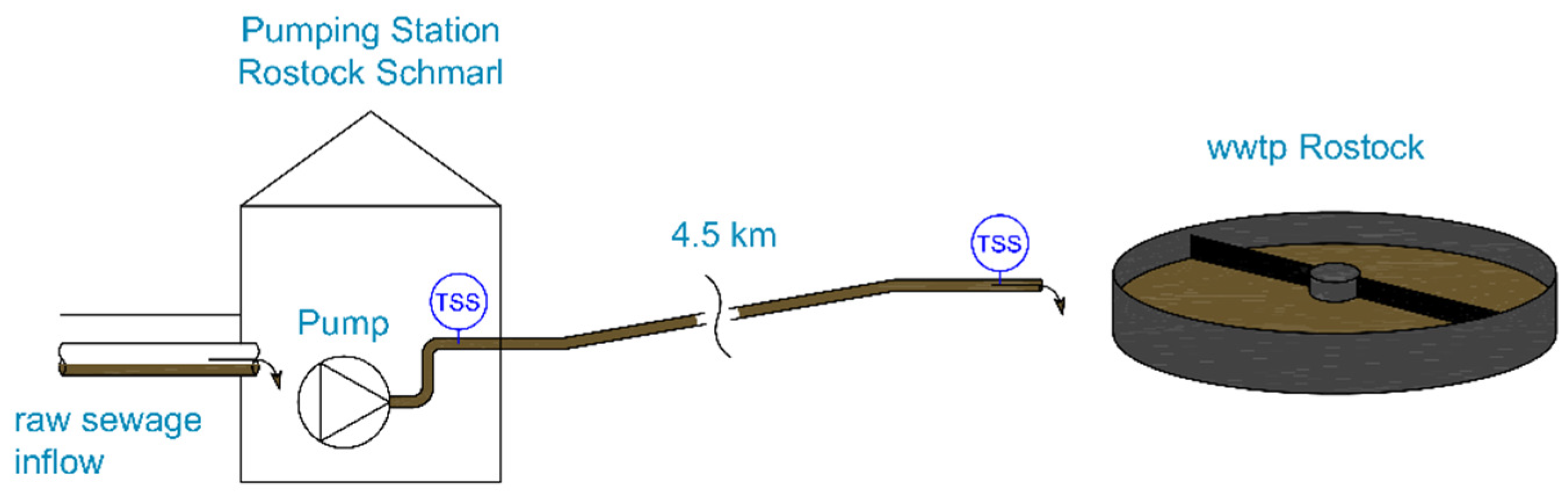
To illustrate the continuous adaptation of the model parameters, Figure 2 shows, exemplarily, the status bar of the sediment transport simulation. At the current simulation time 01:36 p.m. the pumps generate a flow velocity of 0.3 m/s. Figure 2a–d show the simulated values for suspended load (Figure 2a), bed load (Figure 2b), the settling parameter α (Figure 2c), and the erosion parameter d (Figure 2d) over pipe length (4500 m).
3. Results and Discussion
3.1. Evaluation of Model Accuracy
The evaluation of the numerical solution is based on a simple comparison. The reference values were compared to the simulation results. The best solution (minimal deviation to reference values) provides the best parameter set for later simulation of scenarios. The reference values were measured at the pipes end by the calibrated monitoring, see [3]. The simulation was conducted with (i) static ex situ parameters, (ii) static in situ parameters, and (iii) dynamic in situ parameters.
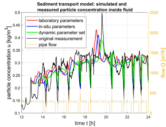
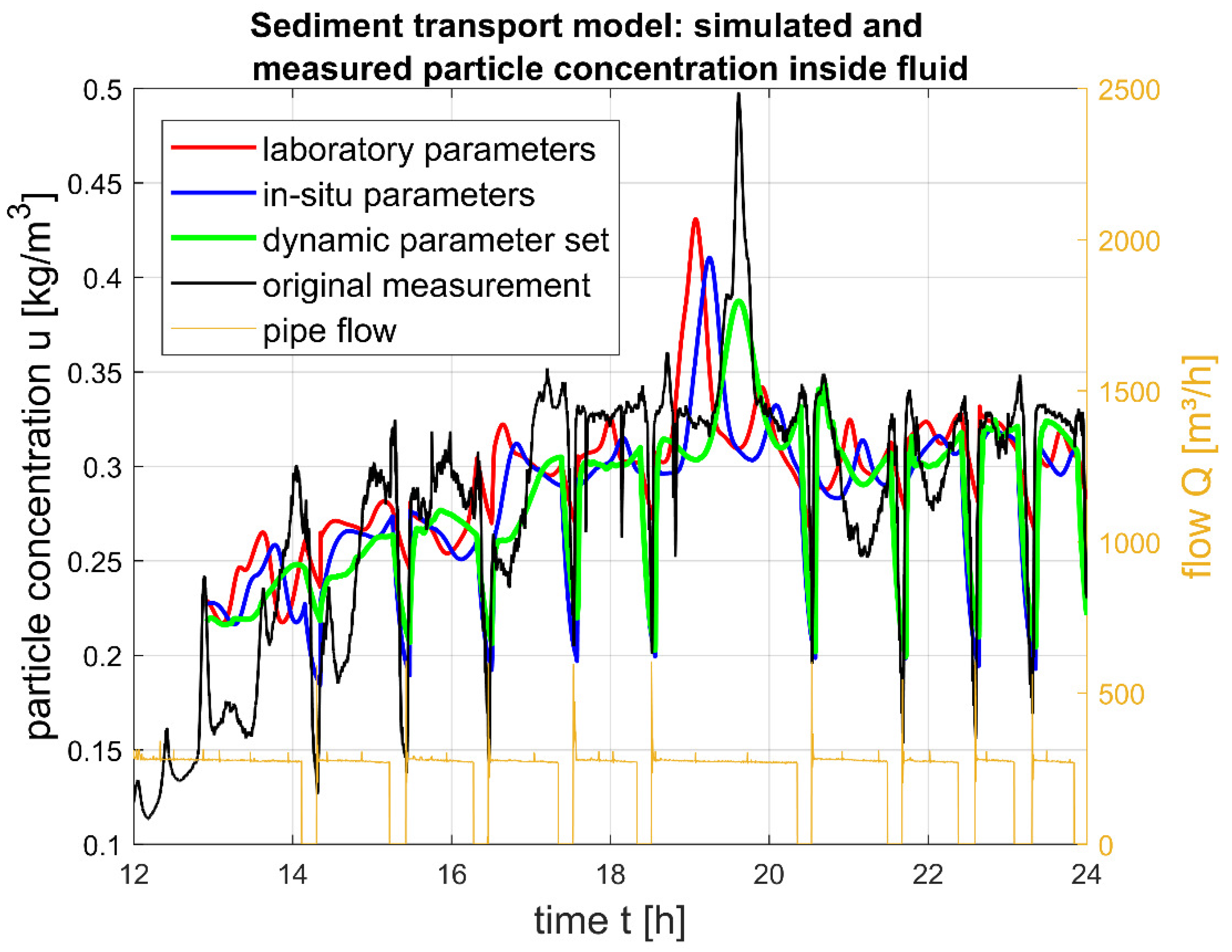
Figure 3 depicts the results of the sediment transport simulation for a typical dry weather inflow at PS-Rostock Schmarl. With the original particle concentration measurement at pipes end representing the reference values (black line). The simulation provides representative results after 13 h, as the pipe is filled with clear water at the beginning of the computation. All three simulations generally follow the measured TSS course. The variable parameter set (green line, , ) only differs marginally from the reference values. The simulation with in situ parameters (blue line, α = 0.0017 s−1, d = 0.0189 s) and laboratory parameters (red line, α = 0.00033 s−1, d = 0.0362 s) differ to larger extent. In particular, particles are transported too fast and reach the end of the pressure pipe too early. This is related to an underestimation of the settling process. The simulated TSS by laboratory parameters never decreases below 0.25 kg/m3, while the original measurement decreases partially below 0.15 kg/m3. So the particles, mostly settle more completely in real life than expected by the laboratory results from [1]. One reason might be in the method (ex situ) itself, as several uncertainties overlay (sampling, experimental setup, and laboratory analysis) and increase the measurement error. The computation with in situ parameters resulted, by far, in better settling prediction, but contains a time shift as well. The simulated curve illustrates the advantage of the real-life measurement with less uncertainties, results in a more precise computation. With the variable parameter set (derived from all in situ parameter sets), a realistic particle concentration profile is simulated. This parameter set will further be used to compute several scenarios.
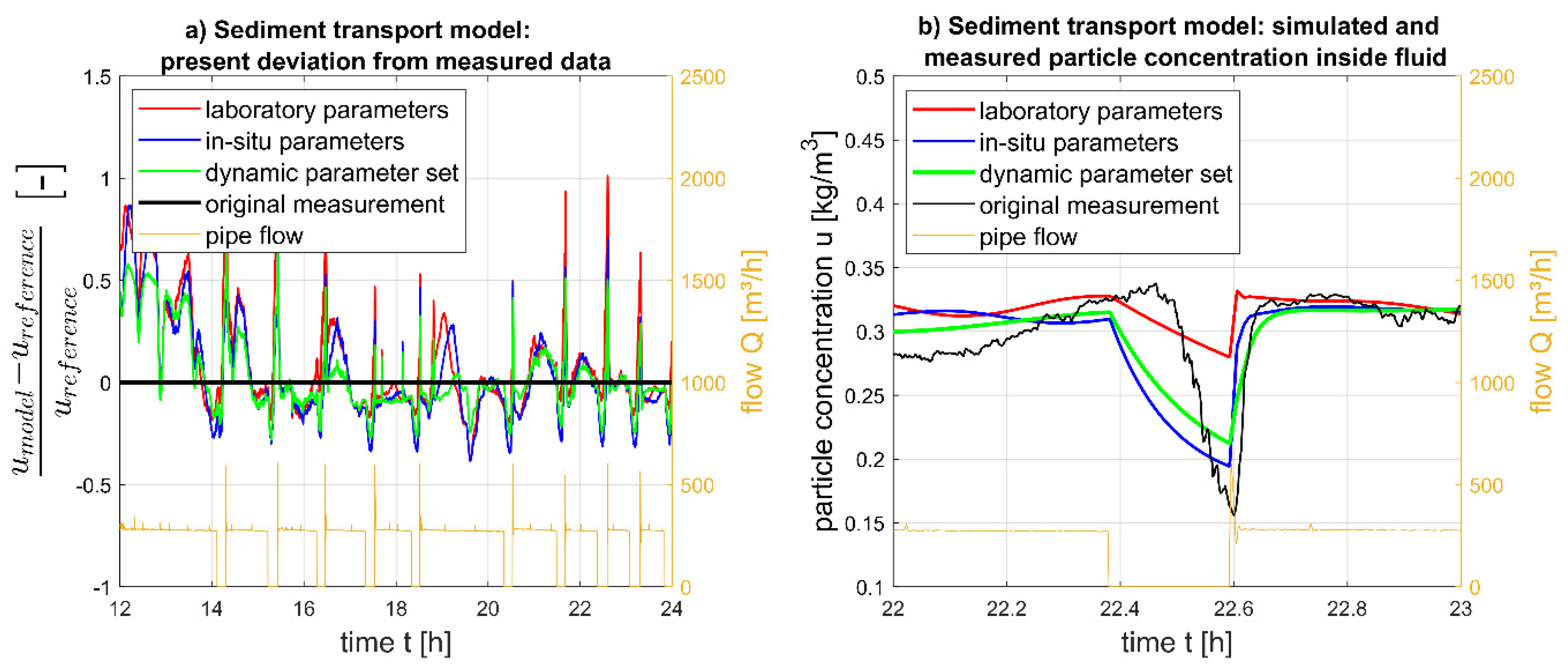
The present deviation to the reference values are shown in Figure 4a and calculated as (umodel − ureference)/ureference. A positive deviation within the settling sequences (Q = 0) remarks an underestimation of the settling process, while reversely a positive deviation within the erosion sequence remarks an overestimation of the real erosion process. Both, under and overestimation occurs within the settling and erosion sequences, with maximum values of ≈+109% (for laboratory parameters) (underestimation of settling sequence). The variable parameter set simulation deviated at a maximum of +75% (underestimation of settling sequence) at the beginning and reduced to ≈+50% during the later simulation.
The largest deviations occur during settling sequences. The negative deviation at the beginning of the settling sequence (see Figure 4a) remarks an overestimation, the particles are settling too fast. Later they are settling too slow, remarked by the positive deviation. Figure 4b shows the simulated particle concentration for an exemplary settling sequence. As one can see, the real settling process (black line) seemed to be delayed. The settling process started significantly after pumps stop (Q = 0). This behavior can be explained by the turbidity measurement. The reference values were measured only in the sensor section (in pipes central region). If the pump process stops, particles settled immediately over the complete pipe section. The particle concentration in the complete fluid section decreases, while it stagnated in the sensor section. Particles settling out of the sensor section were compensated by particles settling into this section. As a result, the reference particle concentration decreases later than expected by the computation.
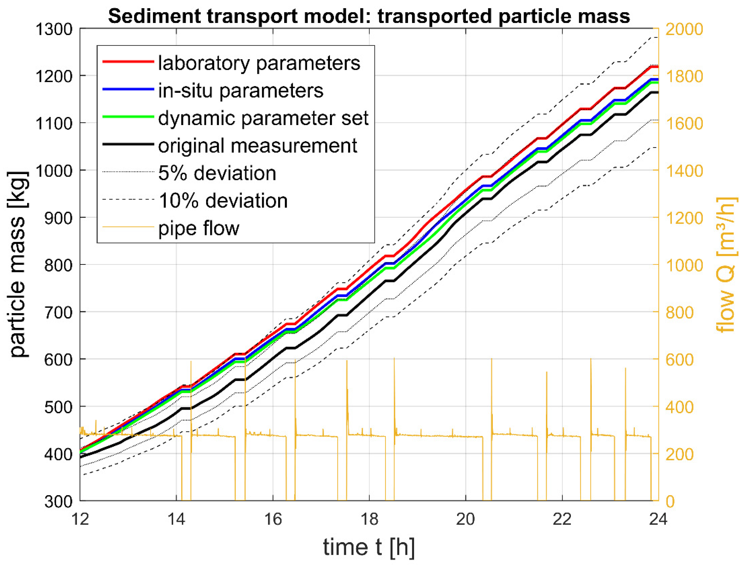
However, the simulated settling illustrates real life conditions, as the computed mass balance relates to the complete fluid section. This results, especially during the pump pauses, in a varying deviation. A trend cannot be detected visually. Therefore, Figure 5 shows the cumulated particle mass, calculated from the measurement and all three simulations. The particle mass, transported through the pipe, amounts to 1164 kg (reference values). All three simulations were within a 10% deviation (±164 kg). The in situ and variable parameter sets were within 5% deviation (±82 kg). Hence, the sediment transport model can be used with the variable parameter set to simulate the particle fluxes inside a pressure pipe appropriately.
3.2. Sediment Transport under Various Regimes
The calibrated sediment transport model offers various possible applications in the field of urban drainage. We concentrate on the investigation of sediment transport inside pressure pipe under different flow regimes. Hence, the simulation of different pump control modes is the basis. Step one: We computed the mean flow velocity over a defined period, by a pump simulation. Step two: We computed the particle transport based on the previously simulated mean flow velocity, by a sediment transport simulation. The simulated pump control modes are summarized in Table 1.
The main control rules from Table 1 represent real life pump control modes of PS Rostock-Schmarl appropriately. The control modes differ mainly in the reduction of the duty. Furthermore, some pump restrictions were added or left out, see Table 1.
The measured inflow and TSS hydrographs at PS Rostock-Schmarl represent the incoming sewage and TSS flow for the pumping simulation. To compare the different pumping strategies, all five control modes were simulated over the same period of 30 days. The results were evaluated for bed load, suspended load, and resulting energy consumption.
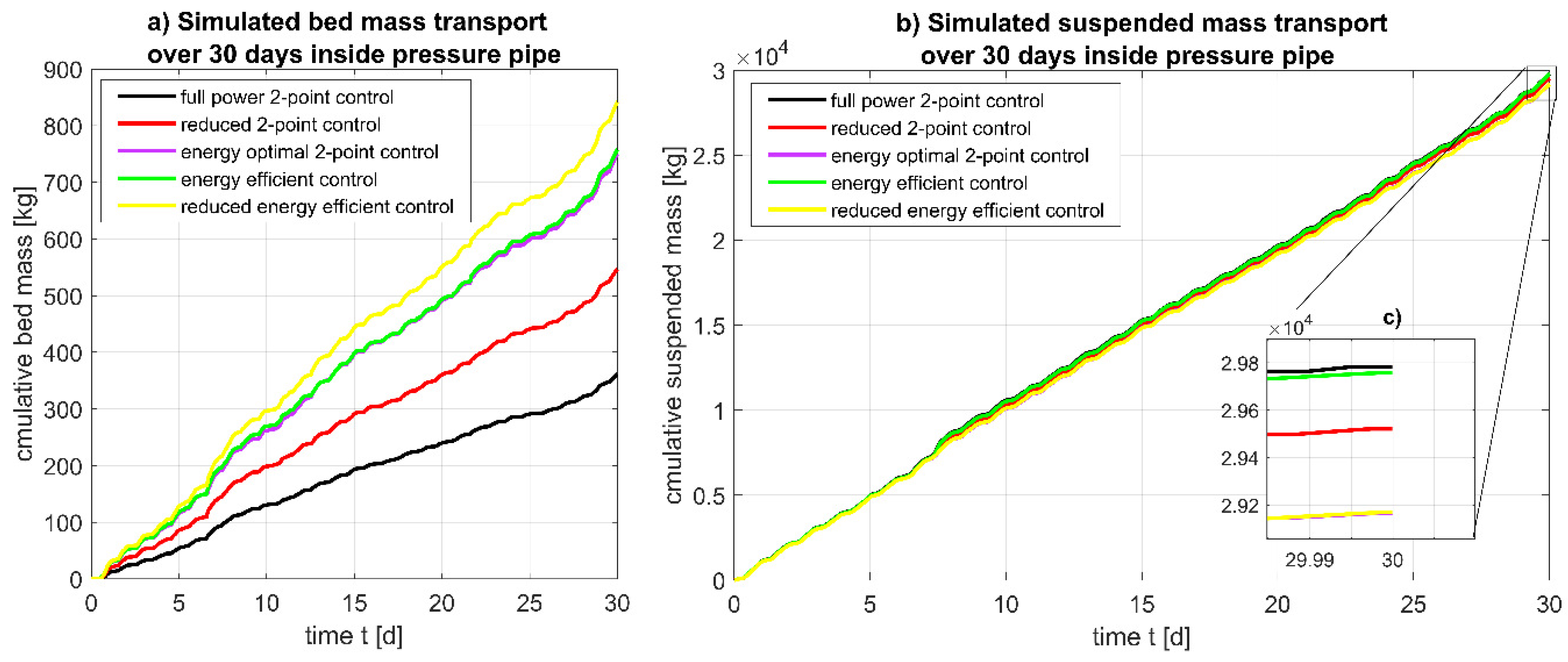
The resulting bed load and suspended load transport is shown in Figure 6. Figure 6a shows the cumulative bed load while Figure 6b,c shows the cumulative suspended load over 30 days simulation. Table 2 summarizes the simulation results for all five pump control modes including the calculated energy demand.
The total transported sediment mass is similar in all five control modes and only differs by ≈2%. In contrast, the ratio between bed load and suspended load varies between control modes. As to be expected, the least amount of bed load was transported within the strongest operation mode: Full power two-point control with ≈360 kg in sum. The suspended load amounts to ≈27,800 kg in full power mode. Hence, the bed load takes only ≈1.3% of the total transported mass (= 28,160 kg) while 98.7% are transported within the suspended load at a flow velocity of ≈0.6 m/s.
This ratio changes due to the weaker control modes on behalf of the bed load. The bed load transport increases with a decreasing duty point (compare to Table 1). However, even at very low flow velocities of ≈0.27 m/s within the energy efficient control modes, the proportion of the bed load transport only amounts up to ≈2.8% of the total transported sediments. This means, a reduction of >50% flow velocity and a loss of ≈80% bed shear stress (from full power two-point control down to energy efficient control, see Table 1) does not results in significant changes of the bed or suspended load transport.
A critical transport limit is reached when the present bed shear stress falls below the critical bed shear stress for eroding sediments. The erosion rate then becomes zero. The least critical limit was calculated based on the results from [2] to ≈ 0.1 m/s flow velocity (≈ 28 L/s flow rate) at a critical bed shear stress of 0.02 N/m2 after 20 min settling. This is below the technical minimum flow possible at PS Rostock-Schmarl of ≈ 53 L/s, which at the same time represents the absolute mean inflow value to the PS. However, the simulation at a duty point of 0.2 m/s flow velocity showed that only 77% of the total sediment mass is transported (compared to 100% sediment transport in full power mode). Applying the calibrated model at a duty point below the technical limitation showed that having specific pure sewage flow velocities down to 0.1 m/s are feasible, but gradually lead to a decrease in transported sediment mass. Apart from this, such a reduction is not feasible for reasons of capacity loss. It is therefore recommended to set the duty point at least above the absolute mean inflow value, or even better to the energy-optimal value. In addition, a flow adjustment should be installed to compensate for inflow peaks, especially when storm runoff is connected. This guarantees both sediment transport and energy savings.
In order to put the sediment transport into context with the energy savings, these were recorded during pump simulation. The simulation of the energy consumption shows a good correlation of the pump simulation with the real system. The power consumption simulated for 30 days under reduced two-point control amounts to ≈10,960 kWh. In the same period, 11,179 kWh are measured in PS Rostock-Schmarl under reduced two-point control. The deviation is only −2%. Concluding, the computed energy consumption can be used to make reliable statements for all five control modes.
Already ≈−9% energy savings were achieved in PS Rostock-Schmarl’s usual operation mode (reduced two-point control) compared to full power two-point control. Further energy savings were obtained by the energy optimal two-point and energy efficient control with ≈−18%. The maximum energy savings of ≈−33% could be achieved with the reduced energy efficient control.
It should be noted that these energy savings were computed for a PS with a very flat system curve. The share of dynamic losses in total pressure losses was only 11% in full power duty point (≈16 m static head to 18.3 m total head loss in duty point = 2.3 m dynamic loss). This proportion decreased with the energy saving control modes to 4%. So, the energy saving potential was low and resulted in moderate energy savings compared to the usual operation mode. The ratio changes in favor of energy saving when greater friction losses occur in the usual duty point of a simple two-point control (e.g., with smaller pipe diameter). However, the reduced flow regime in energy efficient control contribute to the reduction of CO2 emissions and operation costs without dangerously increasing the sedimentation of sewage solids.
3.3. Sediment Transport under Storm Water Inflow
Storm water inflow alter the transport characteristics of the raw sewage, see [1,3]. Sedimentation and erosion are intensified. Storm water inflows are considered by the dynamical adjustment of calibration parameters α and d to the TSS inflow. Hence, the settled mass in the specific grid cell increases faster within pump pauses when storm water inflow enters the cell boundary. Subsequently erosion is intensified when the pumps start up. The critical bed shear stress τcrit increases with the duration of the pump pause, but is not affected by the storm inflow. As the mechanical pre-treatment cleans the inflow from coarse material, it is assumed that the critical bed shear stress value after the pre-treatment is not modified by storm inflow. This assumption was supported by the results from [1]. The laboratory experiments with raw sewage samples from PS Rostock-Schmarl have shown that “the particle spectrum did not change from dry- to wet-weather inflow (…), but rather the proportion of particles, especially in the medium speed fraction” ([1], p. 10). The proportion of the fastest particle class (> 40 mm/s) only increased by 1.19% from dry to wet weather sewage samples. An aggravated erosion was considered by the increased sediment amount on pipes bottom. The erosion process then simply takes longer. An example calculation is given in [2], where the erosion process is prolonged with increasing settling duration.
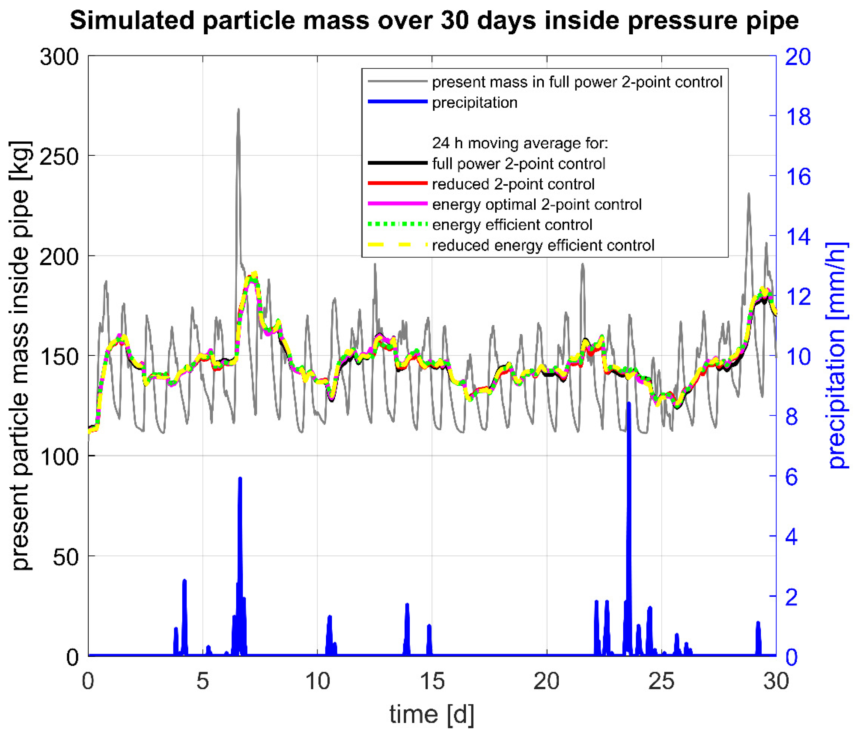
The effect of storm water inflow to sediment transport inside pressure pipe were evaluated for the same 30 days period as described in the previous section. Several rain events are recorded during this period in the catchment area of PS Rostock-Schmarl. Figure 7 shows the present amount of sediments inside the pressure pipe, simulated over 30 days for all five control modes. The present particle mass was calculated as the total sediments quantity in all grid cells per time step (including both suspended and bedload). Figure 6 shows the present particle mass inside the pressure pipe for full power two-point control in detail (grey line) and for better visualization the 24 h simple moving average of the present particle mass of all five control modes (black to yellow lines).
The recorded rain events are shown on the right axis (blue line). Due to the size of the catchment area and the limitation of the connected areas on main roads (see also [3]), not all storm runoffs finally reach the PS. A good example was recorded at day 6. The storm runoff quickly enters the upstream sewer and subsequently the pressure pipe. The present particle mass increases up to ≈270 kg.
Under dry weather inflow, the peaks show the maximum sediment load inside the pipe during the day (at lunch) at ≈160 kg, while the sediment mass decreases in the night down to ≈115 kg.
Due to the 24 h average values, peaks were dampened but it provided the opportunity of supervision. It shows the results of long-lasting trends more clearly. If the moving average value increases constantly without decreasing, permanent deposits forming. However, such a trend cannot be detected. Even the increase in sediment volume due to storm runoff does not lead to a long-term formation of deposits. The sediments mass leveled out at ≈145 kg.
This is, off course, a result of the model calibration with settling parameters α, d, and τcrit. These parameters, calculated from in situ measurements in [3], representing real life conditions inside the pressure pipe. The simulation shows, that even under very low flow velocities, the sediments were transported safely. A permanent deposits formation is prevented by the continuous pump operation regardless of the control mode or the duty point.
4. Conclusions
The paper presents a transport model for 1 D numerical simulation of the sediment transport inside a pressure pipe. The model aims at an exact description of the sediment transport by a limited but case-specific set of transport equations. It is quite simple from a physical point of view. However, an easy but descriptive assessment tool for sediment transport in pressure pipes is available, based on calibration parameter determination by in situ measurements.
The following fields of application are conceivable: Energy-efficient pump control, optimization of sewage disposal and treatment supply to wwtp’s, pollution transport to urban drainage facilities, planning and design of urban drainage systems, and optimization of pipe flushing.
The investigation of hydraulic boundary conditions in pressure pipes under dry weather and storm water inflow have shown in case specific that very low flow velocities and shear stress values are tolerable. Accordingly, the developed energy-efficient pump control with low flow velocities can guarantee the safe disposal of wastewater streams.
Author Contributions
Conceptualization, M.R., J.T. and K.F.; Data curation, M.R.; Formal analysis, M.R. A.F. and K.F.; Funding acquisition, J.T.; Investigation, M.R.; Methodology, M.R., K.F. and J.T.; Project administration, J.T.; Software, A.F., K.F. and M.R.; Supervision, J.T.; Validation, M.R. and A.F.; Visualization, M.R.; Writing—original draft, M.R.; Writing—review & editing, J.T., T.K., A.F. and K.F. All authors have read and agreed to the published version of the manuscript.
Funding
The presented studies are supported by Deutsche Bundesstiftung Umwelt (DBU), Germany (AZ 32253/01).
Acknowledgments
The precipitation data used are available from Germany’s national meteorological service (Deutscher Wetterdienst (DWD)), http://www.dwd.de.
Conflicts of Interest
The authors declare no conflict of interest. The funders had no role in the design of the study; in the collection, analyses, or interpretation of data; in the writing of the manuscript, and in the decision to publish the results.
References
- Rinas, M.; Tränckner, J.; Koegst, T. Sedimentation of Raw Sewage: Investigations for a Pumping Station in Northern Germany under Energy-Efficient Pump Control. Water 2019, 11, 40. [Google Scholar] [CrossRef] [Green Version]
- Rinas, M.; Tränckner, J.; Koegst, T. Erosion characteristics of raw sewage: Investigations for a pumping station in northern Germany under energy efficient pump control. Water Sci. Technol. 2018. [Google Scholar] [CrossRef] [PubMed]
- Rinas, M.; Tränckner, J.; Koegst, T. Sediment Transport in Sewage Pressure Pipes, Part I: Continuous Determination of Settling and Erosion Characteristics by In-Situ TSS Monitoring inside a Pressure Pipe in Northern Germany. Water 2019, 11, 2125. [Google Scholar] [CrossRef] [Green Version]
- Bagnold, R.A. An Approach to the Sediment Transport Problem from General Physics; U.S. Government Publishing Office: Washington, DC, USA, 1966.
- Engelund, F.; Hansen, E. A Monograph on Sediment Transport in Alluvial Streams; Teknisk Forlag: Copenhagen, Denmark, 1967. [Google Scholar]
- Ackers, P.; White, R. Sediment Transport: New Approach and Analysis. J. Hydraul. Div. 1973, 99, 2041–2060. [Google Scholar]
- Engelund, F.; Fredsøe, J. A Sediment Transport Model for Straight Alluvial Channels. Hydrol. Res. 1976, 7, 293–306. [Google Scholar] [CrossRef] [Green Version]
- van Rijn, L.C. Sediment Transport, Part I: Bed Load Transport. J. Hydraul. Eng. 1984, 110, 1431–1456. [Google Scholar] [CrossRef] [Green Version]
- Campisano, A.; Creaco, E.; Modica, C. Numerical modelling of sediment bed aggradation in open rectangular drainage channels. Urban Water J. 2013, 10, 365–376. [Google Scholar] [CrossRef]
- Shirazi, R.H.S.M.; Campisano, A.; Modica, C.; Willems, P. Modelling the erosive effects of sewer flushing using different sediment transport formulae. Water Sci. Technol. 2014, 69, 1198–1204. [Google Scholar] [CrossRef] [Green Version]
- Creaco, E.; Bertrand-Krajewski, J.-L. Numerical simulation of flushing effect on sewer sediments and comparison of four sediment transport formulas. J. Hydraul. Res. 2009, 47, 195–202. [Google Scholar] [CrossRef]
- Correia, L.P.; Krishnappan, B.G.; Graf, W.H. Fully Coupled Unsteady Mobile Boundary Flow Model. J. Hydraul. Eng. 1992, 118, 476–494. [Google Scholar] [CrossRef]
- Bonakdari, H.; Ebtehaj, I.; Azimi, H. Numerical Analysis of Sediment Transport in Sewer Pipe. Int. J. Eng. 2015, 28, 1564–1570. [Google Scholar] [CrossRef]
- Danish Hydraulic Institute (DHI). MOUSE—Pollution Transport Reference Manual; Danish Hydraulic Institute: Hørsholm, Denmark, 2017. [Google Scholar]
- Rossman, L.A. EPANET 2 Users Manual; U.S. Environmental Protection Agency: Cincinnati, OH, USA, 2000.
- Ebtehaj, I.; Bonakdari, H. Evaluation of Sediment Transport in Sewer using Artificial Neural Network. Eng. Appl. Comput. Fluid Mech. 2013, 7, 382–392. [Google Scholar] [CrossRef]
- Azamathulla, H.M.; Ab Ghani, A.; Fei, S.Y. ANFIS-based approach for predicting sediment transport in clean sewer. Appl. Soft Comput. 2012, 12, 1227–1230. [Google Scholar] [CrossRef] [PubMed] [Green Version]
- Bizimana, H.; Altunkaynak, A. A novel approach for the prediction of the incipient motion of sediments under smooth, transitional and rough flow conditions using Geno-Fuzzy Inference System model. J. Hydrol. 2019, 577, 123952. [Google Scholar] [CrossRef]
- Safari, M.J.S.; Danandeh Mehr, A. Multigene genetic programming for sediment transport modeling in sewers for conditions of non-deposition with a bed deposit. Int. J. Sediment Res. 2018, 33, 262–270. [Google Scholar] [CrossRef]
- Roushangar, K.; Ghasempour, R. Estimation of bedload discharge in sewer pipes with different boundary conditions using an evolutionary algorithm. Int. J. Sediment Res. 2017, 32, 564–574. [Google Scholar] [CrossRef]
- Ebtehaj, I.; Bonakdari, H.; Khoshbin, F. Evolutionary design of a generalized polynomial neural network for modelling sediment transport in clean pipes. Eng. Optim. 2016, 48, 1793–1807. [Google Scholar] [CrossRef]
- Fricke, A. Optimale Steuerung und Ihre Anwendungen in der Abwassertechnik (Optimal Control and Its Application in Wastewater Technology). Ph.D. Thesis, University of Rostock, Rostock, Germany, 2015. [Google Scholar]
- Knubbe, A.; Fricke, A.; Ecktädt, H.; Neymeyr, K.; Schwarz, M.; Tränckner, J. Energieeffizienter Betrieb von Abwasserfördersystemen [Energy Efficient Strategies for Wastewater Pumping Systems]. GWF Wasser Abwasser 2014, 155, 640–646. [Google Scholar]
- Tränckner, J.; Bönisch, G.; Gebhard, V.R.; Dirckx, G.; Krebs, P. Model-based assessment of sediment sources in sewers. Urban Water J. 2008, 5, 277–286. [Google Scholar] [CrossRef]
- Rossman, L.A.; Boulos, P.F.; Altman, T. Discrete Volume-Element Method for Network Water-Quality Models. J. Water Resour. Plan. Manag. 1993, 119, 505–517. [Google Scholar] [CrossRef] [Green Version]
- Rossman, L.A.; Boulos, P.F. Numerical Methods for Modeling Water Quality in Distribution Systems: A Comparison. J. Water Resour. Plan. Manag. 1996, 122, 137–146. [Google Scholar] [CrossRef]
Figure 1.
Schematic view of the study side. Total suspended solids (TSS) are measured inside the pressure pipe in pumping station (PS) Rostock-Schmarl and at the outflow side in the wastewater treatment plant (wwtp) Rostock after 4.5 km.
Figure 1.
Schematic view of the study side. Total suspended solids (TSS) are measured inside the pressure pipe in pumping station (PS) Rostock-Schmarl and at the outflow side in the wastewater treatment plant (wwtp) Rostock after 4.5 km.

Figure 2.
Status panel of the sediment transport simulation. (a) present suspended load inside the pressure pipe at each grid position. (b) present bed load inside the pressure pipe at each grid position. (c) present settling parameter α inside the pressure pipe at each grid position. (d) present erosion parameter d inside the pressure pipe at each grid position.

Figure 3.
Results of the sediment transport simulation. Particle concentration measured and simulated with laboratory, in situ, and dynamic parameters with slightest deviation.
Figure 3.
Results of the sediment transport simulation. Particle concentration measured and simulated with laboratory, in situ, and dynamic parameters with slightest deviation.

Figure 4.
Results of the sediment transport simulation. (a) present deviation from all three simulated parameter sets. (b) settling sequence detail.
Figure 4.
Results of the sediment transport simulation. (a) present deviation from all three simulated parameter sets. (b) settling sequence detail.

Figure 5.
Results of the sediment transport simulation. Cumulative particle mass transport measured and simulated with laboratory, in situ, and dynamic parameters.
Figure 5.
Results of the sediment transport simulation. Cumulative particle mass transport measured and simulated with laboratory, in situ, and dynamic parameters.

Figure 6.
Sediment transport simulation for five different pumping modes over 30 days. Cumulative bed mass (a) and suspended mass (b) transport.
Figure 6.
Sediment transport simulation for five different pumping modes over 30 days. Cumulative bed mass (a) and suspended mass (b) transport.

Figure 7.
Sediment transport simulation for five different pumping modes over 30 days. Present particle mass inside pressure pipe on left axis and precipitation data on right axis (rain events are measured by a German Weather Service (DWD) meteorological station located inside the catchment area).
Figure 7.
Sediment transport simulation for five different pumping modes over 30 days. Present particle mass inside pressure pipe on left axis and precipitation data on right axis (rain events are measured by a German Weather Service (DWD) meteorological station located inside the catchment area).


Table 1.
Simulated pump control modes with significant settings.
| Pump Data | Simulated Pump Control Modes | ||||
|---|---|---|---|---|---|
| Full Power 2-Point Control | Reduced 2-Point Control | Energy Optimal 2-Point Control | Energy Efficient Control | Reduced Energy Efficient Control | |
| Flow in duty point (L/s) | 166.5 | 100 | 76.5 | 76.5 | 76.5 |
| Flow velocity in duty point (m/s) | 0.6 | 0.35 | 0.27 | 0.27 | 0.27 |
| Head loss in duty point (m) | 18.3 | 17 | 16.7 | 16.7 | 16.7 |
| Bed shear stress in duty point (N/m2) | 0.95 | 0.32 | 0.2 | 0.2 | 0.2 |
| Power Input in Duty Point (kW) | 55 | 33.5 | 22.5 | 22.5 | 22.5 |
| Power start-up * | yes | yes | yes | yes | no |
| Adjusted pump flow to inflow ** | no | no | no | yes | no |
| Parallel pumping from critical sump level | yes | yes | yes | yes | yes |
| Forced operation at least 1/hour | yes | yes | yes | yes | yes |
* Pumps start-up to maximum power over one minute before regulating down to duty point in each pump sequences, ** If the inflow exceeds the present duty point, pump regulates up to the inflow rate.
Table 2.
Resulting bed and suspended load for five different pumping modes.
| Simulated Pump Control Modes | |||||
|---|---|---|---|---|---|
| Full Power 2-Point Control | Reduced 2-Point Control | Energy Optimal 2-Point Control | Energy Efficient Control | Reduced Energy Efficient Control | |
| Total sediment transport (kg) | 30,140 (100%) | 30,066 (100%) | 29,918 (100%) | 30,517 (100%) | 30,011 (100%) |
| Bed load transport (kg) | 360 (1.2%) | 546 (1.8%) | 750 (2.5%) | 757 (2.5%) | 841 (2.8%) |
| Suspended load transport (kg) | 29,780 (98.8%) | 29,520 (98.2%) | 29,170 (97.5%) | 29,760 (97.5%) | 29,170 (97.2%) |
| Power consumption (kWh) | 11,982 | 10,960 (−9%) | 9868 (−18%) | 9874 (−18%) | 7974 (−33%) |
© 2020 by the authors. Licensee MDPI, Basel, Switzerland. This article is an open access article distributed under the terms and conditions of the Creative Commons Attribution (CC BY) license (http://creativecommons.org/licenses/by/4.0/).
Share and Cite
MDPI and ACS Style
Rinas, M.; Fricke, A.; Tränckner, J.; Frischmuth, K.; Koegst, T. Sediment Transport in Sewage Pressure Pipes, Part II: 1 D Numerical Simulation. Water 2020, 12, 282. https://doi.org/10.3390/w12010282
AMA Style
Rinas M, Fricke A, Tränckner J, Frischmuth K, Koegst T. Sediment Transport in Sewage Pressure Pipes, Part II: 1 D Numerical Simulation. Water. 2020; 12(1):282. https://doi.org/10.3390/w12010282
Chicago/Turabian StyleRinas, Martin, Alexander Fricke, Jens Tränckner, Kurt Frischmuth, and Thilo Koegst. 2020. "Sediment Transport in Sewage Pressure Pipes, Part II: 1 D Numerical Simulation" Water 12, no. 1: 282. https://doi.org/10.3390/w12010282
Note that from the first issue of 2016, this journal uses article numbers instead of page numbers. See further details here.