Article

Application of a Self-Organizing Map of Isotopic and Chemical Data for the Identification of Groundwater Recharge Sources in Nasunogahara Alluvial Fan, Japan

Institute for Rural Engineering, National Agriculture and Food Research Organization, Ibaraki 305-8609, Japan
*
Author to whom correspondence should be addressed.
Water 2020, 12(1), 278; https://doi.org/10.3390/w12010278
Submission received: 26 November 2019 / Revised: 15 January 2020 / Accepted: 16 January 2020 / Published: 18 January 2020
(This article belongs to the Special Issue Use of Water Stable Isotopes in Hydrological Process)

Abstract

:
Paddy rice fields on an alluvial fan not only use groundwater for irrigation but also play an important role as groundwater recharge sources. In this study, we investigated the spatial distribution of isotopic and hydrochemical compositions of groundwater in the Nasunogahara alluvial fan in Japan and applied a self-organizing map (SOM) to characterize the groundwater. The SOM assisted with the hydrochemical and isotopic interpretation of the groundwater in the fan, and clearly classified the groundwater into four groups reflecting the different origins. Two groundwater groups with lower isotopic ratios of water than the mean precipitation values in the fan were influenced by the infiltration of river water flowing from higher areas in the catchments and were differentiated from each other by their Na+ and Cl concentrations. A groundwater group with higher isotopic ratios was influenced by the infiltration of paddy irrigation water that had experienced evaporative isotopic enrichment. Groundwater in the fourth group, which was distributed in the upstream area of the fan where dairy farms dominated, showed little influence of recharge waters from paddy rice fields. The findings of this study will contribute to proper management of the groundwater resources in the fan.

Graphical Abstract

1. Introduction

Alluvial fans are important lowland areas in Japan because approximately 70% of the total land area of Japan is mountainous or hilly. Vast paddy rice fields are situated on alluvial fans, which occupy more than half (54%) of Japan’s lowland area [1]. River water is usually diverted at the apexes of such alluvial fans and then delivered through a network of irrigation canals to each paddy rice field by gravity [2]. Alluvial fans are also vital aquifer systems that support local agricultural, industrial, and socio-economic development worldwide, wherever groundwater is utilized as an important water resource [3]. Aquifers of permeable sand and gravel formed in alluvial fans are vulnerable to contamination from the surface, and therefore interactions between surface water and groundwater can even affect hydrochemical processes (e.g., [4,5,6,7]). In addition, the infiltration of irrigation water contributes considerably to groundwater recharge [8] and also produces complex groundwater flows in paddy-dominant alluvial fans. For the sustainable use of groundwater resources in fans, it is important to understand these groundwater flows and recharge sources.
Environmental isotopes and hydrochemical data are powerful tools for investigating groundwater flow conditions (e.g., [9,10]), including hydrogeological investigations of alluvial fans (e.g., [8,11,12]). A multifaceted analysis using a suite of tracers (multi-tracer approach) can be effectively used to interpret complex groundwater flow conditions that cannot be observed directly. Multivariate analysis methods, such as principal component analysis and factor analysis, which allow for the dimensionality of multiple hydrochemical indicators to be reduced and features of groundwater flow conditions to be extracted, have been widely applied in hydrological system analysis (e.g., [13,14,15]). However, these multivariate analyses are generally based on linear principles and they cannot overcome difficulties arising from biases due to the complexity and nonlinearity of the datasets and from inherent correlations between variables [16]. Therefore, a self-organizing map (SOM) approach, a neural network–based pattern analysis with unsupervised learning, has recently been applied to map changes in groundwater levels and chemistry in space and time (e.g., [17,18,19,20]). An SOM, which can cluster a set of hydrochemical data into two or more independent groups, is superior to other statistical tools because it can: (1) deal with system nonlinearities, (2) be developed from data without requiring mechanistic knowledge of the system, (3) handle noisy or irregular data and be easily and quickly updated, and (4) be used to interpret and visualize information of multiple variables or parameters [16,21].
In this study, we performed an environmental isotopic and hydrochemical investigation of the Nasunogahara alluvial fan in central Japan, which was formed by several rivers and has a vast area (400 km2), about 40% of which is used for rice production. The paddy rice fields are irrigated by both river water and groundwater. The river water is transmitted through the Nasu canal system, one of the three major canals for paddy field irrigation in Japan. The yield of groundwater pumped out of the fan for irrigation is the second largest for agricultural use in Japan [22]. The groundwater in this fan also emerges as numerous springs in the central to lower part of the fan. These springs support a unique ecosystem inhabited by freshwater fish (three-spined stickleback, Gasterosteus aculeatus) that has been designated as a natural monument [23]. The groundwater in the alluvial fan is recharged not only by direct percolation of precipitation but also by the infiltration of water from the rivers that flow across the fan and water from irrigated paddy rice fields [24]. Thus, a part of the irrigation water used in the alluvial fan, whether derived from surface water or groundwater, returns from the paddy rice fields to the aquifer.
Previous studies of groundwater in this area have focused on spatio-temporal variations in the groundwater quality [25,26], groundwater nitrate dynamics [27], and the groundwater budget, as simulated by a 2D horizontal model [28]. Stable isotope ratios of water have been effectively used to identify recharge sources of the groundwater in the central part of the fan [24], but the applicability of the method to the whole fan remains to be demonstrated, and how different recharge sources influence the flow of groundwater in the aquifer is still unclear. Therefore, further research is needed to provide information for farmers and other local residents to enable sustainable use of groundwater in the fan and conservation of the springs. Therefore, we measured multiple environmental isotopes and the hydrochemistry of groundwater in the Nasunogahara alluvial fan during two paddy cultivation periods, one with and one without irrigation. We then applied an SOM based on our results to identify the groundwater recharge sources and interpret groundwater flow through the aquifer system.

2. Study Area

2.1. Location, Land Use, and Water Use

The Nasunogahara alluvial fan in central Japan was formed by the Naka, Sabi, Kuma, and Houki rivers, which flow out of the mountainous region to the northwest of the fan (Figure 1). The alluvial fan extends over an area of approximately 400 km2 and is bounded by the Naka River along its eastern edge and the Houki River along its western edge. The flow in the upper reaches of the Sabi and Kuma rivers is usually underground, but these rivers emerge above ground in the central part of the fan and join the Houki River in the toe of the fan. Then, the Houki and Naka rivers converge in the southeasternmost part of the fan. As a result, the Nasunogahara fan is spindle-shaped, different from most alluvial fans. The topography of the fan is mainly flat; its elevation ranges from 60 to 560 m a.s.l., although scattered hills dissected by numerous streams occupy the lower part of the fan. The slope near the fan apex is 3/100, and the slope in the central and lower parts of the fan is 1/100; the average slope is 1.6/100. Paddy rice fields cover about 40% of the fan surface [29] and are densely distributed in the central and lower parts (Figure 1). About one-quarter of the paddy rice fields are irrigated by surface water diverted from the rivers, and the rest are irrigated by groundwater. In 2008, 240 million m3 of groundwater from the fan was used for agriculture [22]. Livestock farms (mostly dairy farms) are located mainly in the upper part of the fan, where there is less groundwater available for irrigation. The mean air temperature and annual precipitation from 1981 to 2010, measured at Kuroiso weather station (343 m a.s.l) (Figure 1), were 11.7 °C and 1526 mm, respectively.

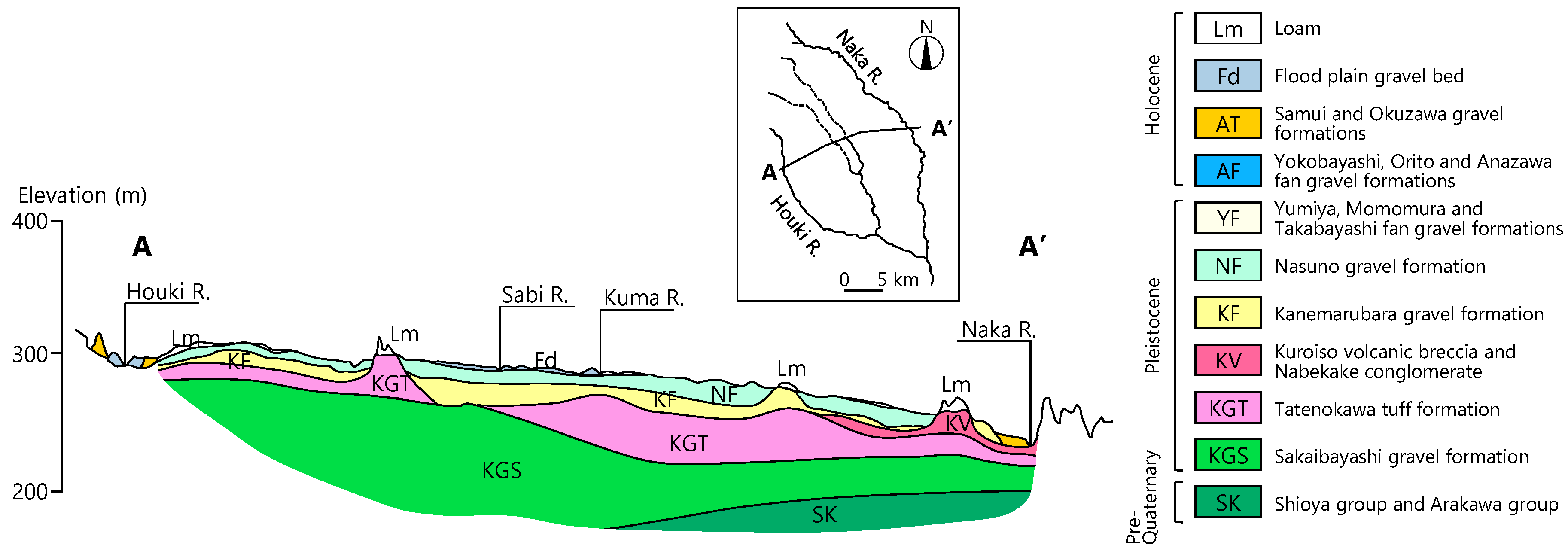
2.2. Hydrogeological Settings

The Nasunogahara alluvial fan consists mostly of Quaternary deposits overlying a basement composed of pre-Quaternary green tuff and mudstone (Shioya and Arakawa groups). In order of decreasing depth, the Sakaibayashi gravel formation, Tatenokawa tuff formation, Kuroiso volcanic breccia, Nabekake conglomerate, Kanemarubara gravel formation, Nasuno gravel formation, the Samui and Okuzawa gravel formations, and a flood plain gravel bed overlie the basement rocks (Figure 2).
An unconfined aquifer is in the flood plain gravel bed and the Samui and Okuzawa formations; in this aquifer, the groundwater table is higher during summer and disappears during winter. A second unconfined aquifer in the Nasuno gravel formation supplies most of the groundwater used for irrigation; it typically has a high hydraulic conductivity of 10−4 to 10−3 m/s [31,32]. The Tatenokawa tuff formation is impermeable and the gravels of overlying formations cover a paleotopography of hills and valleys on the upper surface of the Tatenokawa tuff. The Sakaibayashi gravel formation underlies the Tatenokawa tuff formation and is a confined aquifer. In this study, groundwater samples were collected from depths down to 30.3 m in wells installed in the first and second unconfined aquifers, as described in Section 3.1. The groundwater level of the fan begins to rise in April, reaches a maximum in October, and then declines through March, echoing changes in precipitation [24]. Groundwater levels are thus high from April to September, the paddy rice irrigation period, suggesting that the groundwater may be recharged by paddy irrigation water.

3. Methods

3.1. Sample Acquisition

Many hand-dug wells for paddy irrigation (as well as for upland crop irrigation and domestic use) are distributed across the Nasunogahara alluvial fan, although there are a few wells in the upper part of the fan (Figure 1). We collected samples for the analyses of stable isotopic composition, radon radioisotope (222Rn), and major ion concentrations of water from wells, river waters, and paddy waters, both during the irrigation period (IP, 15–18 May 2018) and during the non-irrigation period (NP, 4–7 March 2019). In the IP, groundwater was collected from 124 wells, but in the NP, some of the wells had dried up because of a drop in the groundwater level (white circles in Figure 1), so groundwater was collected from only 98 wells. The ground elevation of the wells ranged from 134 to 417 m a.s.l., and the well depth ranged from 3.3 to 30.3 m, with an average depth of 9.6 m below ground level. Toward the apex of the fan, the wells were deeper, and toward the toe of the fan, they were shallower. The mean depths of groundwater in the wells in the IP and NP were 3.8 and 2.5 m, respectively. Therefore, isotopic and chemical compositions of groundwaters were considered to be the same regardless of water depth. An acrylic well bailer was used to collect groundwater samples from the wells. Paddy waters were collected from the irrigation water inlet and outlet of seven paddy rice fields only in the IP. Spring waters were collected at six sites (SP1–6) in the IP and three sites (SP4–6) in the NP. Some springs dried up in the NP because of the drop in the groundwater level. A polyethylene cup or EVA (ethylene-vinyl acetate copolymer) bucket were used to sample the paddy and spring waters. River water samples were collected from each of the four rivers (Naka, Kuma, Sabi, and Houki rivers), either from the bank or from a bridge, using an EVA bucket. A relatively low rainfall was observed and the maximum daily rainfalls in and before the IP and NP were 8 and 14 mm, respectively. Therefore, the collected river waters were close to baseflow conditions. Rainwater was collected at site P1 (321 m a.s.l.; Figure 1) from 14 March 2018 to 21 August 2019 (527 days) and site P2 (179 m a.s.l.) from 9 August 2018 to 21 August 2019 (377 days) at a mean interval of 33 days in rain collectors designed, following recommendations described in International Atomic Energy Agency (IAEA)/Global Network of Isotopes in Precipitation (GNIP) [33], to prevent water re-evaporation. The electrical conductivity (EC) of the sampled surface water and groundwater was measured by using a portable EC sensor (TOA-DKK, WM-32EP, Tokyo, Japan) immediately after the sampling. All water samples for chemical and isotopic analyses were transferred to clean polyethylene vials and brought to the laboratory of the Institute for Rural Engineering, National Agriculture, and Food Research Organization (Ibaraki, Japan), where they were filtered through syringe filters with a polytetrafluoroethylenemembrane (0.45 μm) and stored in a refrigerator until analysis.

3.2. Analysis of Environmental Isotopic and Hydrochemical Compositions

Major ions (Na+, K+, Mg2+, Ca2+, Cl, NO3, SO42−) were quantified using ion chromatography (TOA-DKK, ICA-2000, Tokyo, Japan) using multicomponent standard solutions. Nitrate (NO3) is reported as the nitrate-nitrogen (NO3-N) concentration. Alkalinity was determined using titration to pH 4.8 and is reported as HCO3. For all water samples, errors in the cation–anion charge balance were less than 5%. 222Rn, which is a radioactive gas generated by the decay of 226Ra in geological strata, is soluble in water and has a half-life of 3.8 days. The 222Rn concentration in groundwater finally reaches radioactive equilibrium. It reaches 92% of the value at secular equilibrium after two weeks underground. Using these characteristics, 222Rn is often used as a target tracer to investigate the hydrological aspects of groundwater (e.g., estimation of infiltration from surface water to aquifers [34] and groundwater flow rate [35]), because far more 222Rn is contained in groundwater than in surface water. The radioactivity of 222Rn in samples was analyzed using a liquid scintillation counter (Packard, 2250 CA, CT, USA) after extraction with toluene within one week after collecting the water, and the concentrations of 222Rn were calculated based on the count rate [36]. The stable isotopic compositions of the water were measured using a cavity ringdown spectrometer-based water isotope analyzer (Picarro, L2140-i, Santa Clara, CA, USA). They were reported with respect to Vienna Standard Mean Ocean Water (VSMOW) and are described here in “delta” notation as δ18O and δ2H (in parts per thousand, ‰). Three working standards calibrated by international measurement standards were used for the analysis of δ18O and δ2H. The analytical precision in this study was ±0.05‰ for δ18O and ±0.50‰ for δ2H. The deuterium excess (d-excess, used to indicate the kinetic fractionation effect of evaporation [37]) of each water sample was calculated as d-excess = δ2H − 8δ18O [38]. The Mann–Whitney U test, which is applicable to non-normally distributed variables, was used to assess the independence of the measured isotopic and hydrochemical compositions between the IP and NP.

3.3. SOM

An SOM is an unsupervised training algorithm of an artificial neural network model developed by Kohonen [39]. An SOM can project high-dimensional target data onto a low-dimensional format (typically a two-dimensional grid map called a “feature map”) [40]. Therefore, it is an effective and powerful analysis tool for the detection of data characteristics using pattern classification and visualization [16]. An SOM consists of an input layer and an output layer. The output layer often consists of a rectangular grid map with a hexagonal lattice (“nodes”). Each node in the output layer has a vector of coefficients associated with the input data, the so-called reference vector (also referred to as the weight vector and the codebook vector). The vectors can be obtained using iterative updates during a training phase consisting of three main procedures: competition between nodes, selection of a winning node, and updating of the reference vectors [40,41].
The determination of the SOM structure (calculation of the total number of nodes and the ratio of the number of map rows to the number of map columns) is an important step in the application of an SOM. If the number of nodes (i.e., map size) is too small, it might not explain some important differences that should be detected. Conversely, if the map size is too big, the differences between adjoining nodes are too small [42]. The optimal number of nodes in an SOM can be selected by using the heuristic rule m = 5 n , where m denotes the total number of nodes and n is the number of samples in the data set [40,43]. The ratio of the number of rows to the number of columns in the feature map is determined by calculating the square root of the ratio of the largest eigenvalue of the correlation matrix of the input data to the second-largest eigenvalue [19]. In this study, the eigenvalues were obtained using principal component analysis of the input dataset. Normalization of the data was necessary prior to the application of the SOM to ensure that all values of the chemical parameters were given similar importance. The results of the SOM application are sensitive to the method used for data pre-processing because the SOM is trained to organize itself according to the Euclidean distances between input data [40]. In this study, all variables of the input data were transformed to have a range of 0 to 1 such that they would have equal importance in the formation of the SOM.
For clustering the trained SOM, several methods, each with advantages and disadvantages, are available. Agglomerative clustering and partition clustering result in clear groupings on the trained map, whereas application of a U-matrix (unified distance matrix), which is commonly used to create a rough visualization of the classification, may not define clear boundaries (e.g., [44]). Ward’s agglomerative hierarchical clustering (Ward’s method) is an easy way to cluster nodes on the trained map because it is not necessary in this method to determine the optimum number of groups before performing the clustering calculations [42]. Ward’s method has been commonly used to subdivide the trained map into several groups according to the similarity of the reference vectors of the nodes (e.g., [43,45]). Thus, Ward’s method was applied in this study to identify groups on the trained map.
In this study, the input layer of the SOM consisted of 11 chemical and isotopic parameters (δ2H, δ18O, 222Rn, and the major ion concentrations) of groundwater samples collected at 124 and 98 wells in the IP and NP, respectively. In accordance with the heuristic rules described above, a feature map with 72 (9 × 8) nodes was selected. The “kohonen” package in the R statistical software environment (version 3.5.1, Vienna, Austria) [46] was used to implement the SOM. Default values of the package parameters (e.g., learning rate and size of the neighborhood) were used. The observed hydrochemical and isotopic data of the groundwater in the fan were preprocessed by the proposed SOM, and then the groundwater data were spatially clustered into different homogeneous groups on the trained map. To identify the groundwater recharge sources, the hydrochemical and isotopic compositions of the groups were plotted on various types of diagrams (i.e., hexa-diagrams, a trilinear diagram, a δ18O–δ2H scatter diagram, and spatial distribution maps) and compared.

4. Results

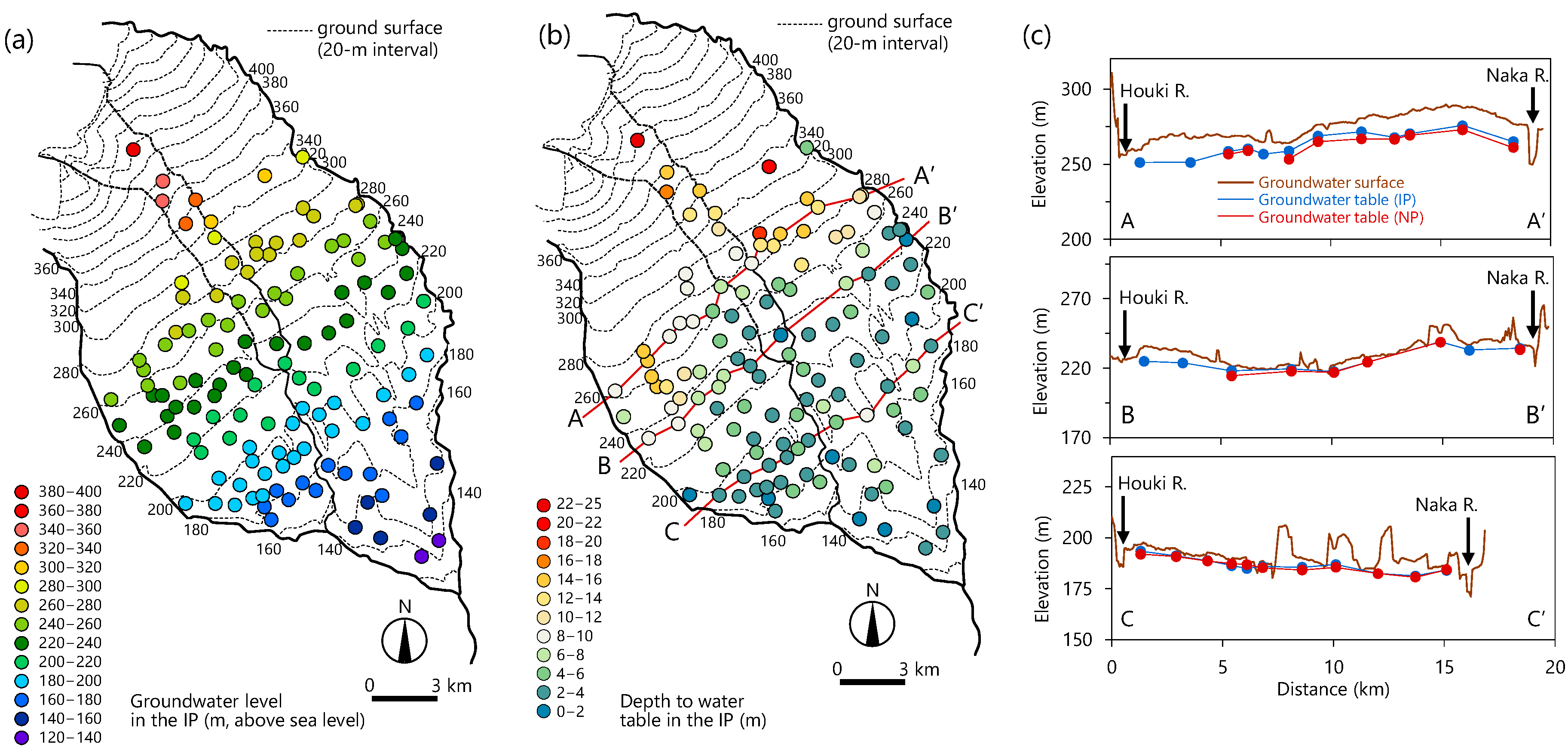
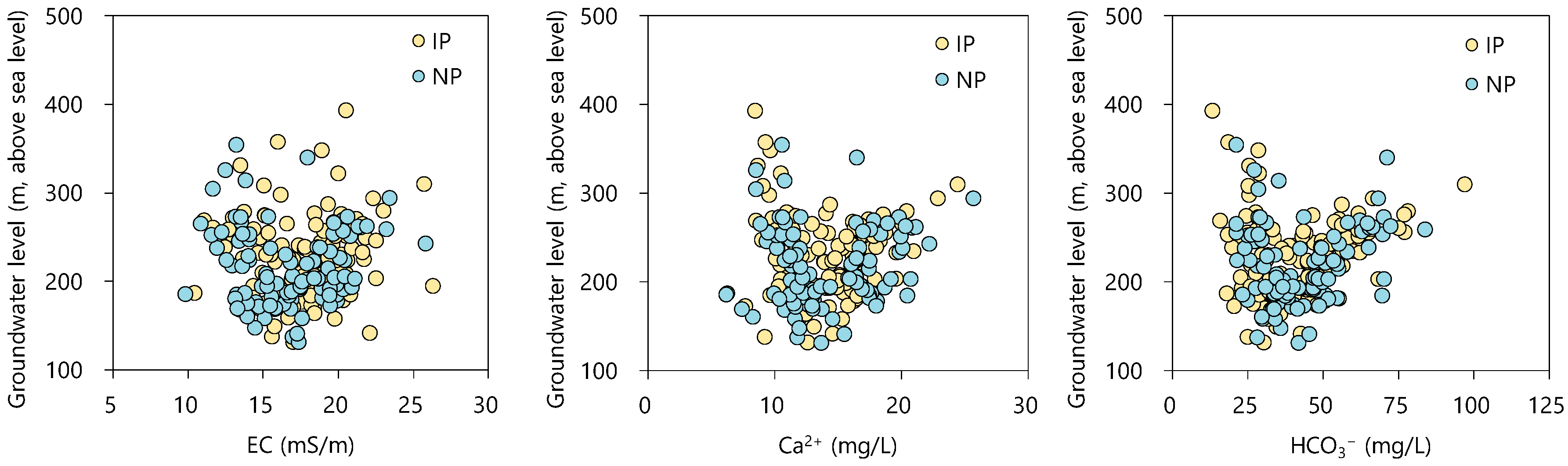
4.1. Groundwater Level

We mapped groundwater levels, depth to the water table, and cross-sections of the water table in Figure 3. The groundwater table was almost parallel to the ground surface of the fan, which sloped toward the southeast, and the groundwater flowed in the same direction.
The depth to the groundwater table in the upper to middle part of the fan (from the apex to about 260 m above sea level) was relatively large. In this area, the Sabi and Kuma rivers were losing streams and hence recharged the aquifer. The terrace cliffs on the right bank of the Naka River along the eastern edge of the fan varied from several meters to several tens of meters in height (Figure 3c), and therefore, the river bed of the Naka River was lower than the groundwater table. This means that there was no recharge from the Naka river to the aquifer. The riverbed of the Houki River was about 10 m higher than the groundwater surface near the middle part of the fan. The Houki River recharged the aquifer in this part and the infiltrated river water flowed in the downstream direction in accordance with hydraulic gradient, whereas the groundwater table became higher toward the toe of the fan. The lower part of the fan, where the water level became closer to the ground surface, corresponded to the groundwater discharge area.

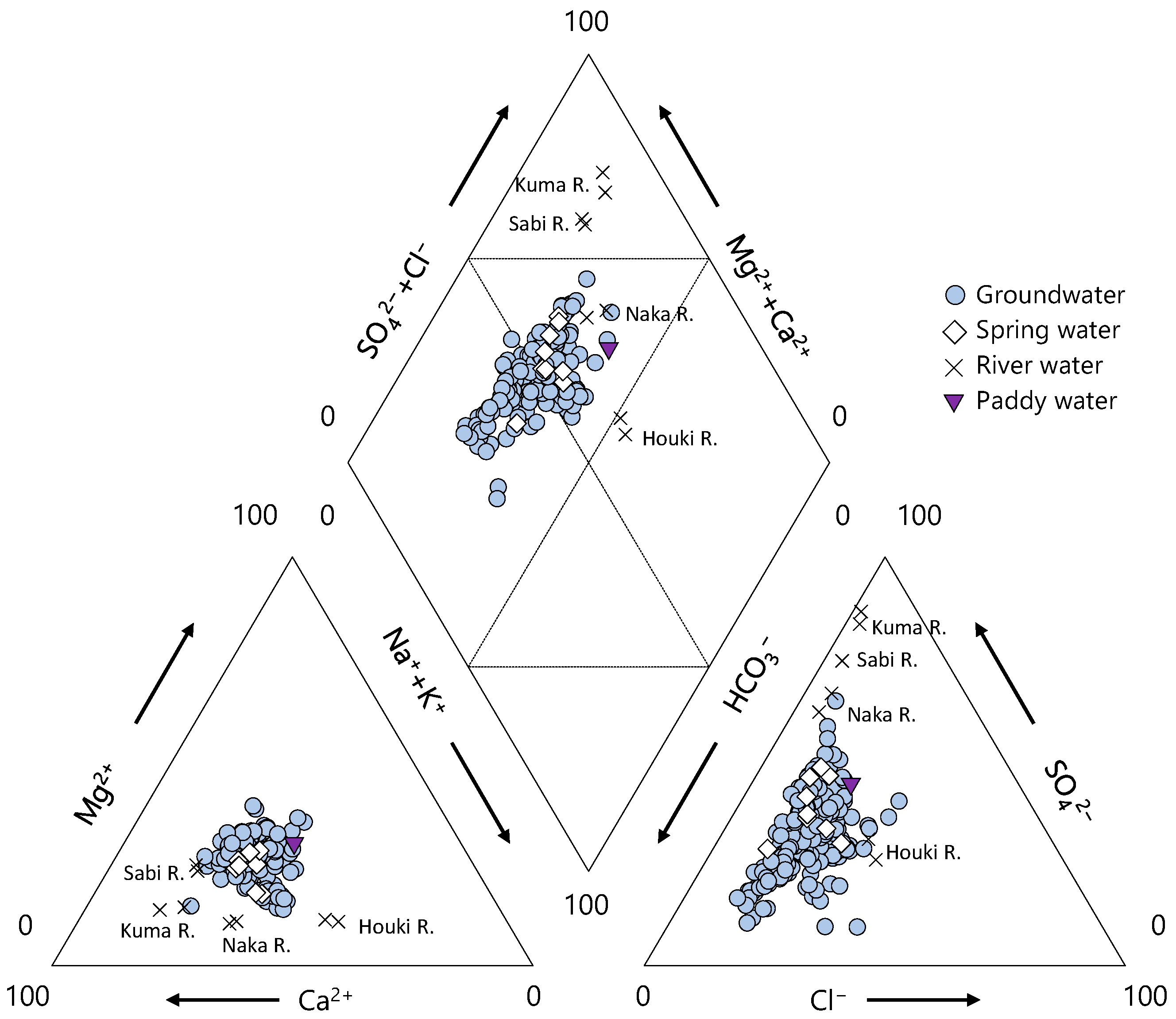
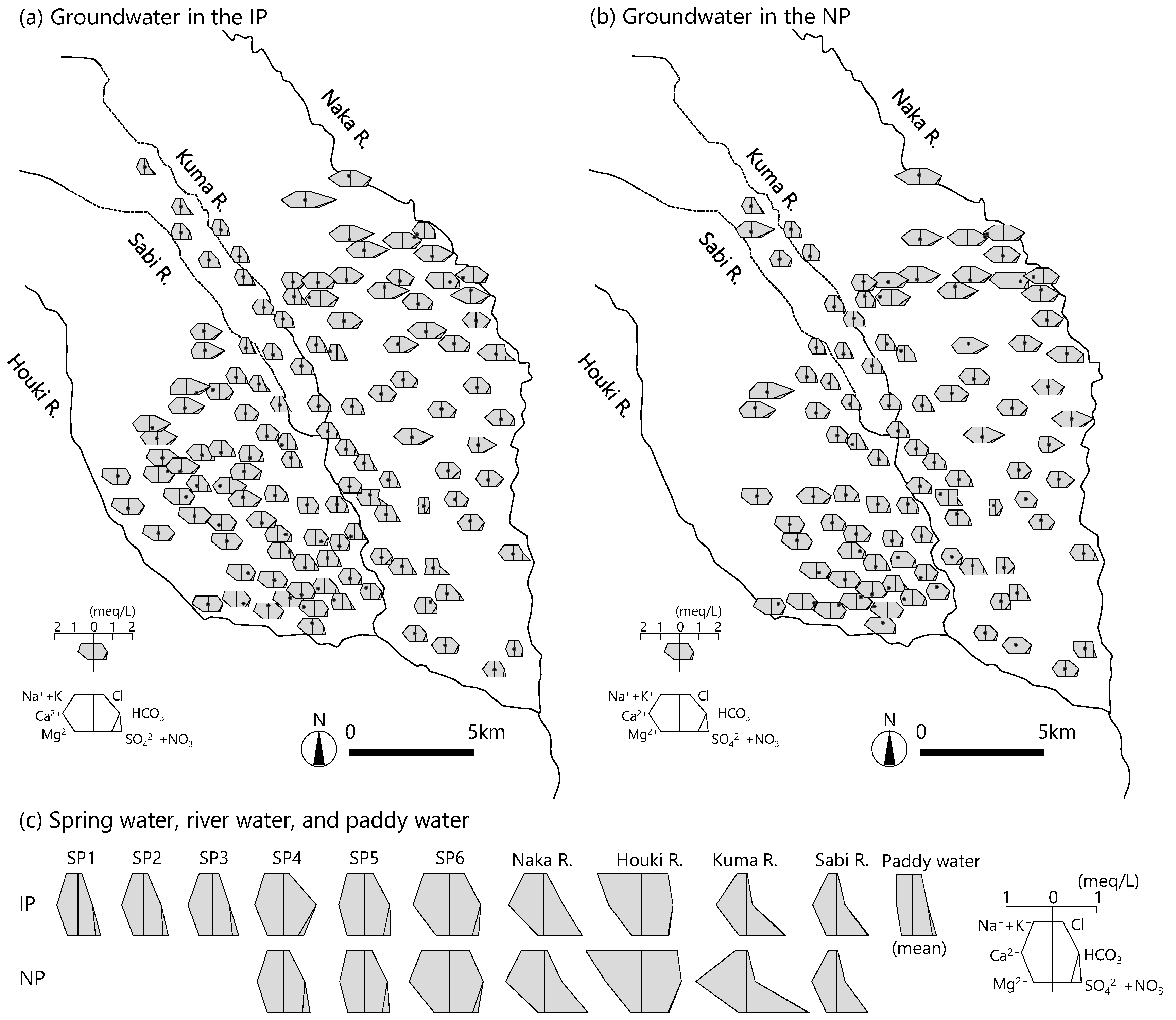
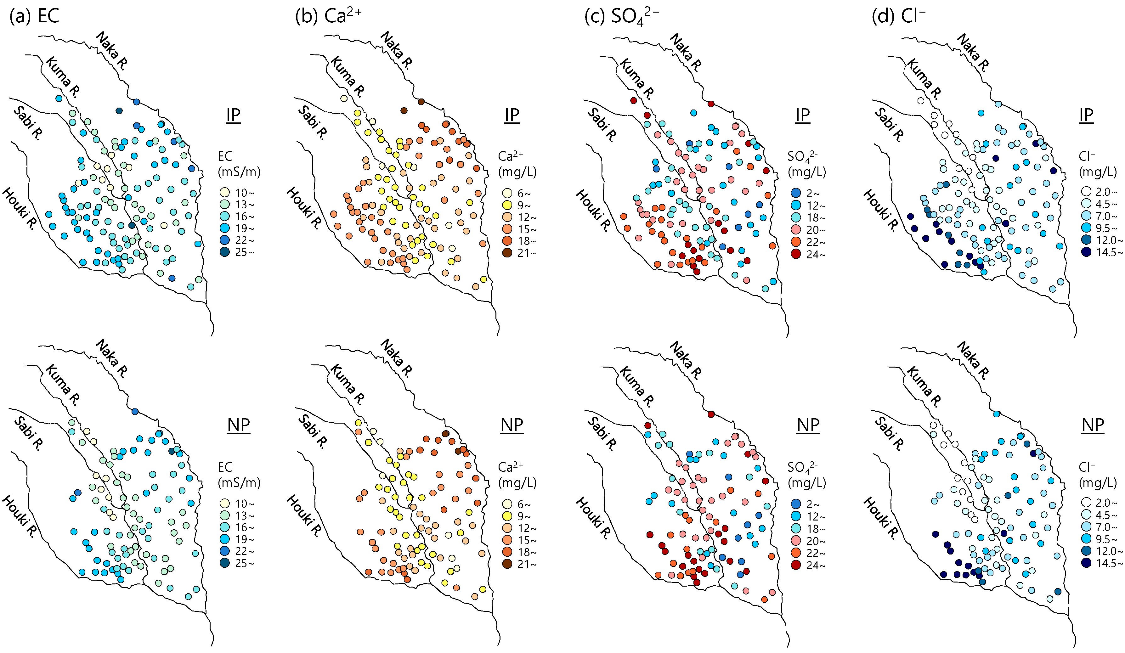
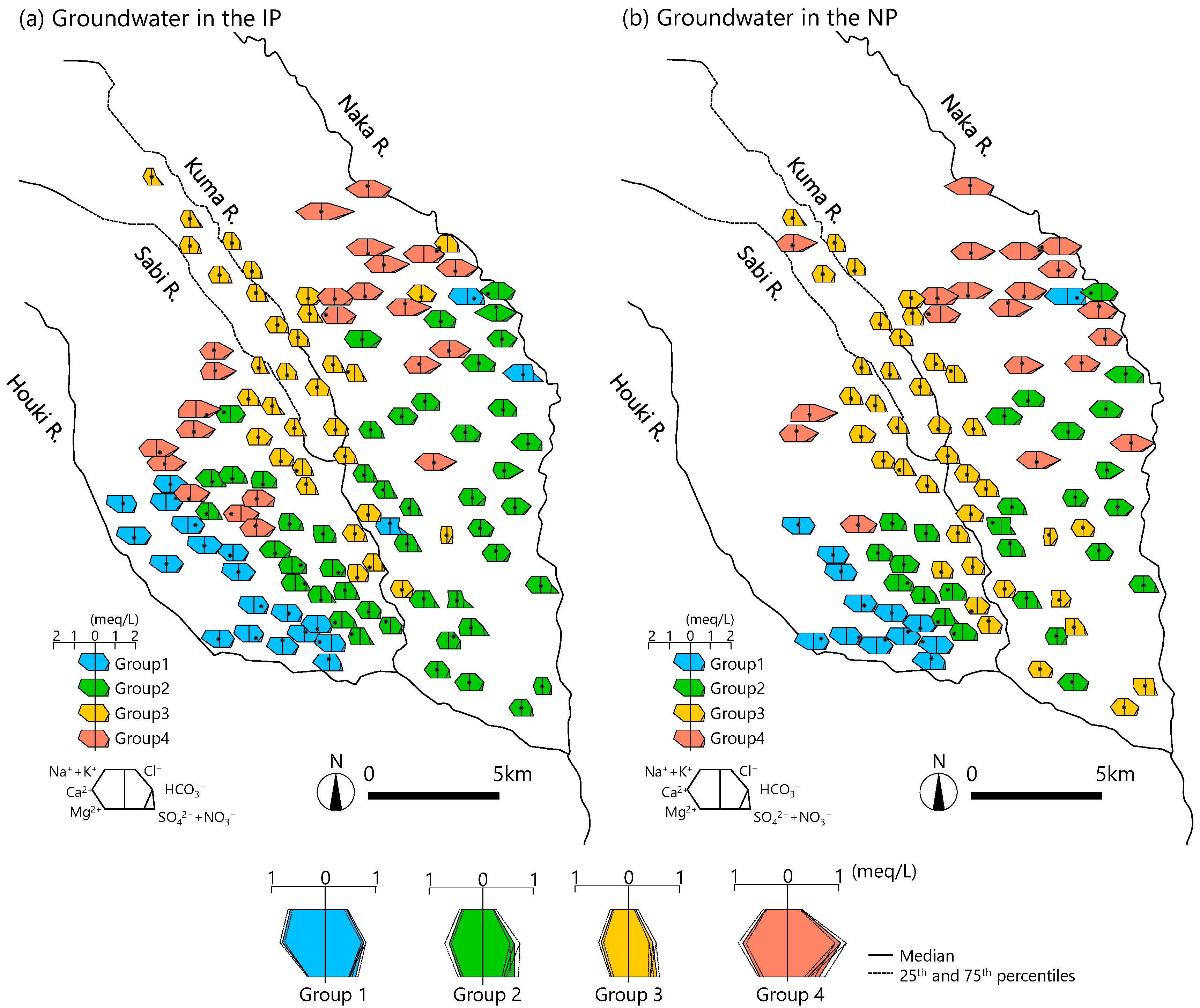
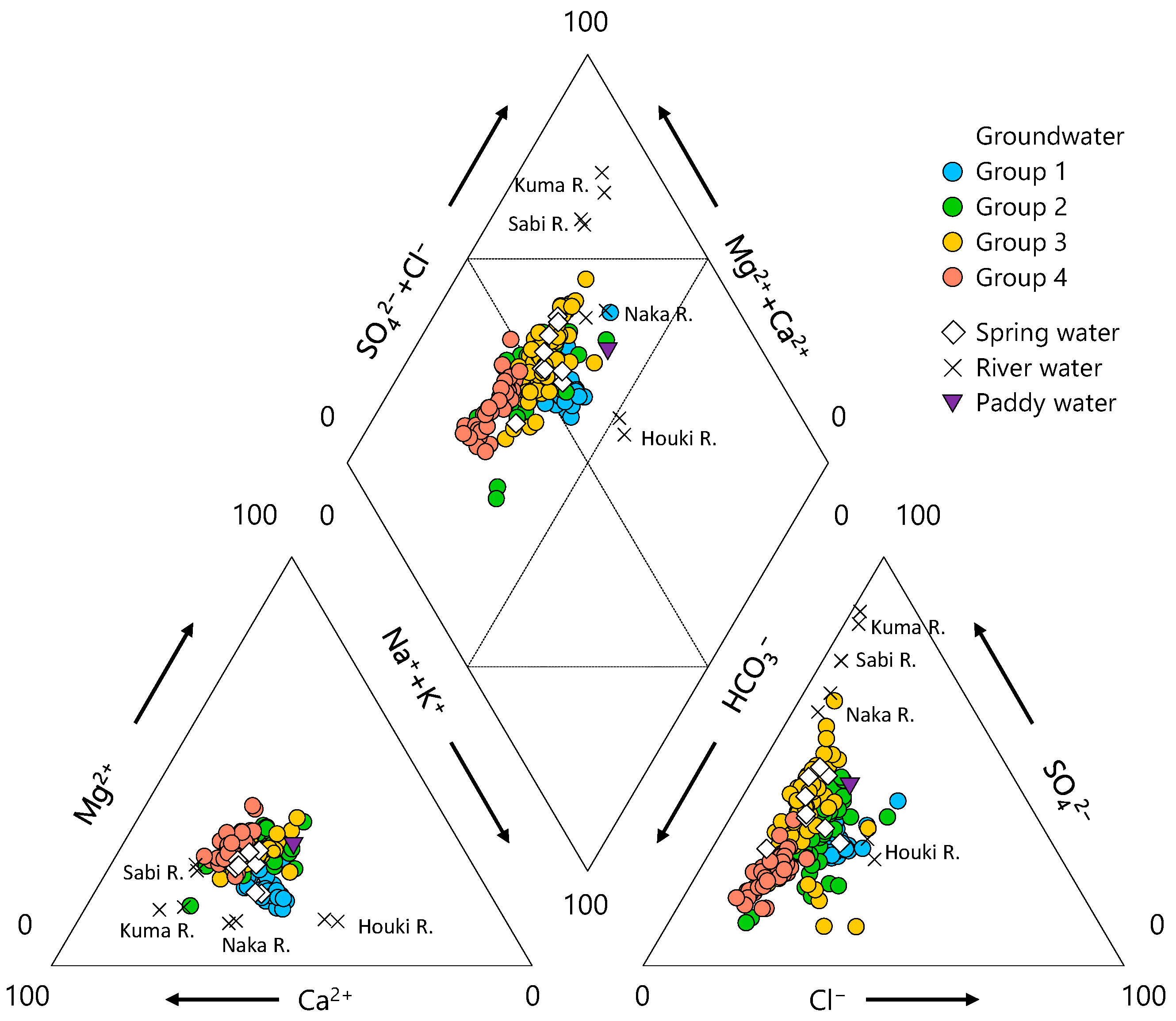
4.2. Chemical Compositions

Analytical results of the chemical and isotopic parameters of the groundwater, along with those of spring water, paddy water, river water, and rainwater, are shown in Table 1. Four groups of the groundwater were classified using the SOM, as described later in Section 4.4. The chemical compositions of the groundwater, spring water, and river water are shown as a Piper (trilinear) diagram in Figure 4 and as hexa-diagrams in Figure 5. The Ca-HCO3 type typically indicates shallow fresh groundwater, while Na-HCO3 type typically indicates weathering and ion exchange processes. As shown by the key diagram and hexa-diagrams, some groundwater samples had a Ca-HCO3-to-Ca-SO4-Cl-type composition, whereas the Ca-HCO3-type composition was dominant. Groundwater samples were plotted near the center of the cation ternary diagram (Figure 4), suggesting little variability in the relative proportions of these cations. The anion ternary diagram indicated larger variability among samples: Groundwater samples were mostly HCO3-type water, whereas some groundwater samples were scattered between HCO3 and SO42− types.
Table 2 shows the matrix of the Pearson correlation coefficients for EC and major ions of all groundwater samples. Ca2+, which is highly correlated with EC, is a major controlling factor of EC. A strong positive correlation between Ca2+ and HCO3 indicates that a dominant water type of the groundwaters in this aquifer was Ca-HCO3 type. Concentrations of Ca2+ and HCO3 in aquifers of alluvial fans increased due to mineralization induced by a water–rock interaction during the groundwater flow process (e.g., [47]). Figure 6 shows the relationships between EC, Ca2+, and HCO3 of the groundwater with groundwater level. These values did not increase with the downstream direction in the fan. The spatial distribution of the hexa-diagrams in Figure 5 indicates that the chemical compositions varied greatly depending on the location, especially the distances from the rivers.
Figure 7 illustrates the spatial distributions of EC and the concentrations of the three characteristic ions Ca2+, SO42−, and Cl of groundwater in the IP and NP. The spatial distribution of EC, which was low along the Sabi and Kuma rivers in the central part of the fan, was very consistent with previous survey results [25,48]. Along these two rivers, Ca2+, like EC, was relatively low, whereas SO42− was relatively high. In contrast, Cl concentrations were higher along the western edge of the fan near the Houki River than elsewhere in the fan. As is shown by the hexa-diagrams and ternary diagrams, the Naka, Sabi, and Kuma River waters were characterized by large SO42− contents, whereas the Houki River water samples had higher Na+ and Cl concentrations than the waters from the other rivers. Spring waters were plotted between the HCO3 and SO42− types on the anion ternary diagram; SP1, SP2, and SP3 were characterized by larger SO42− contents, as indicated by their hexa-diagram shapes. No significant seasonal difference between the IP and NP was observed in the chemical compositions of the river and spring waters.

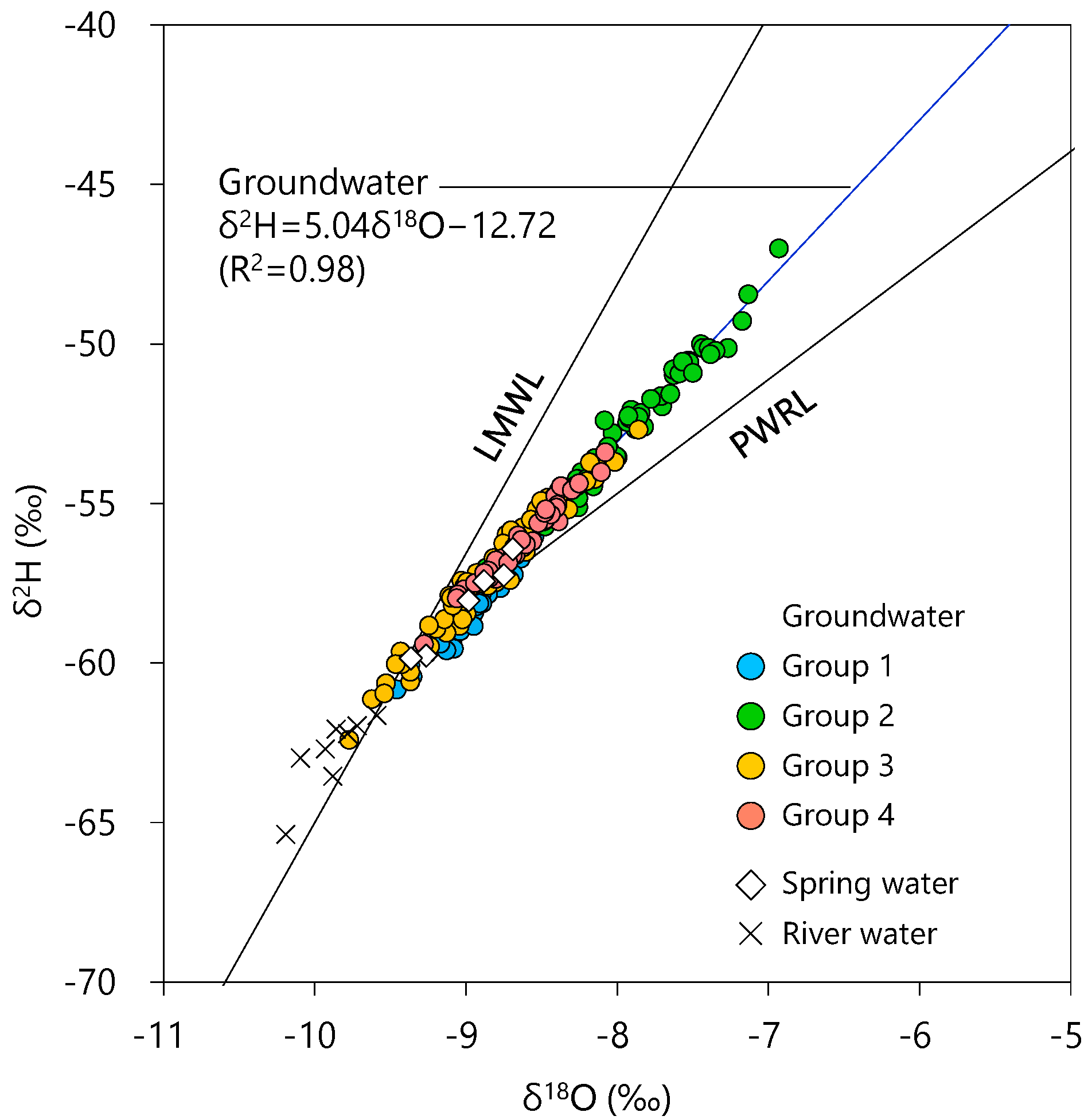
4.3. Isotopic Compositions

The relationship between δ18O and δ2H (δ18O–δ2H scatter diagram) in all water samples is shown in Figure 8. In rainwater collected at sites P1 and P2, δ18O and δ2H varied over relatively wide ranges, from −12.9‰ to −3.1‰ and from −85‰ to −5‰, respectively. The local meteoric water line (LMWL) in this study area was determined to be δ2H = 8.48δ18O + 20.09. The slope of the LMWL was slightly larger than the global meteoric water line (GMWL) slope of 8 [49] and the slope of the meteoric water line on the Pacific Ocean side in Japan (7.8) [50]. The weighted means of δ18O and δ2H (weighted using the precipitation amount during the sampling time interval) were −8.3‰ and −54‰ at P1 and P2, respectively; these values, which were plotted below the LMWL, reflect the low d-excess value of rainwater in summer in Japan [51] because the region of the Nasunogahara fan receives more precipitation in summer than in winter.
The slope of the regression line between δ18O and δ2H of paddy waters, denoted as PWRL in Figure 8, was 3.6. The plots of the paddy water data deviated from the LMWL and the d-excess value of the paddy water (−2.2‰) was extremely low compared to those of the groundwater, rainwater, and river water (Table 1). Generally, kinetic fractionation of oxygen and hydrogen isotopes during evaporation causes the remaining water to become enriched in the heavier isotopes (18O and 2H); as a result, trends with slopes ranging from 4 to 7 are seen on the δ18O–δ2H scatter diagram, whereas the equilibrium isotopic fractionation line lies near the LMWL and has a slope close to 8 [52]. If there is no rain, irrigation water is supplied to the paddy fields almost every day and is affected by evaporative enrichment, even in just one day. Paddy waters affected by evaporative isotopic enrichment would have higher isotopic ratios and lower d-excess values [53] and effects the isotopic compositions in groundwater [54]. In this study, paddy waters collected at paddy field outlets had higher isotopic ratios than those collected at the inlets because evaporative isotopic enrichment occurred during the residence time of the water in the paddy rice fields. The slope of the regression line fitted to all groundwater data was 5.04, between those of the LMWL and the PWRL (Figure 8b). The isotopic ratios of the river water samples were smaller than those of groundwater samples and plotted near the LMWL.
The spatial distributions of δ18O, d-excess, and the 222Rn concentration in groundwater in the IP and NP are shown in Figure 9. The groundwater along the Sabi and Kuma rivers had comparatively low δ18O (less than −8.5‰) and high d-excess values (more than 12.0‰), whereas groundwater in the southeastern part of the fan had high δ18O (more than −8.0‰) and low d-excess values (less than 11.0‰). Compared with the IP, the domain with a high δ18O and low d-excess values in the southeastern fan shrank in the NP. Spatial differences in the 222Rn concentration in groundwater were indistinct, although concentrations in the NP were higher than those in the IP. The 222Rn concentration in waters of the four rivers was close to zero (Table 1).

4.4. SOM and Clustering Results

Figure 10 shows the component planes of the hydrochemical and isotopic parameters finally obtained after iterative training of the SOM. Each component plane shows the value of one component of the reference vector in each of the 72 nodes. Visualization of the data using component planes is helpful for finding interrelationships among the different parameters [21]. For example, the component plane patterns of Na+ and Cl were visibly similar; both had larger values in the lower-left and smaller values in the upper-left part of the plane (Figure 10). The component planes of several other parameter combinations (e.g., δ18O–δ2H, Ca–HCO3, and Mg2+–NO3-N) also showed similar patterns (Figure 10), whereas the component planes of SO42−, K+, and 222Rn did not exhibit any similarity with those of other parameters.
The SOM nodes were subdivided into four groups (groups 1 to 4, comprising 34, 73, 72, and 43 groundwater samples, respectively) according to the dendrogram produced by the hierarchical cluster analysis (Figure 11). Figure 12 shows the spatial distributions of the color-coded hexa-diagrams of the four groups in the IP and NP. Group 1 was mostly distributed near the Houki River, which flows along the western edge of the fan. Group 2 was distributed in the central and lower parts of the fan. Group 3 was distributed along the Sabi and Kuma rivers. Group 4 was distributed across the middle part of the fan.
The EC of group 3 groundwater was lower than that of the other groups (Table 1), indicating that it contained lower amounts of dissolved components. Groundwater in groups 1 and 4 had higher EC than groundwater in groups 2 and 3. In particular, concentrations of Na+ and Cl were notably higher in group 1, whereas those of Ca2+ and HCO3 were higher in group 4. The mean NO3-N concentration was the highest in group 4, but all groundwater samples in this study had nitrate concentrations below the standard level of 10 mg/L NO3-N in Japan. The width of each hexa-diagram is an approximate indication of the total ionic content. Thus, the hexa-diagram width of group 3, which had a low EC, was small, whereas the hexa-diagram widths of groups 1 and 4, which had higher ECs, were large (Figure 12). Chemical compositions of groundwaters in the four groups, spring water, and river water are shown as a trilinear diagram in Figure 13. Groundwater samples of group 4 were mostly HCO3-type water, whereas those of groups 1 to 3 tended to be scattered between HCO3 and SO42 types. In addition, the relative abundance of Cl in group 1 samples was somewhat large.
The δ18O–δ2H scatter diagram of groundwater in the four groups is shown in Figure 14. The groundwater in each of the four groups had characteristic δ18O and δ2H values: group 2 waters had the highest values, followed by waters of groups 4 and 1, and group 3 waters had the lowest values (Figure 14, Table 1). Group 2 waters had the lowest d-excess value and group 3 waters had the highest d-excess value.

5. Discussion

5.1. Influence of Recharge Sources on Groundwater Hydrochemical and Isotopic Compositions

It has been pointed out that shallow groundwater in the Nasunogahara alluvial fan is recharged by multiple sources, including the infiltration of rainwater, river water, and paddy irrigation water (e.g., [24]). The isotopic ratios of groundwater in this study, which were plotted as an elongated cluster between the LMWL and the PWRL in the δ18O–δ2H diagram (Figure 8), also indicate a mixture of groundwaters recharged from three different sources. The fact that the isotopic ratios of the groundwater were plotted between the LMWL and PWRL is strong evidence that groundwater in the fan was influenced by the infiltration of not only rainwater but also paddy irrigation water (Figure 8). In addition, the comparison between groundwater levels and ground surface elevations indicated that there was infiltration from the Houki, Sabi, and Kuma rivers to the aquifer (Figure 3). The isotopic ratios of river waters (mean values of four rivers of −9.9‰ for δ18O and −63‰ for δ2H) were much less than the weighted means of rainwater (see Section 4.3) (Figure 8). The reason for the lower ratios of these river waters was that the rivers gathered precipitation that falls at high altitude in the mountains, which had lower isotopic ratios because of the isotopic altitude effect. The isotopic ratios of some groundwater samples were lower than the weighted mean rainwater δ18O and δ2H values, suggesting that these samples represented a mixture of waters with low isotopic ratios. We therefore inferred that the groundwaters in the western part and upper part of the fan were affected by the infiltration of waters from the Houki River, and the Kuma and Sabi rivers, respectively. The river waters contained baseflows supplied from the mountainous watersheds, but 222Rn concentrations of river waters were low. This indicates that dissolved 222Rn in river waters was lost through dispersion to the atmosphere and radioactive decay before reaching the fan. It had been expected that the 222Rn concentration of the groundwater near the rivers decreased due to river water infiltration, but the concentrations were not lower than those far away from the rivers (Figure 9). This means that the residence time of infiltrated waters to reaching sampling wells was more than two weeks, which were required to reach radioactive equilibrium.
The hydrochemical data also implied that infiltration of river water recharged some groundwaters. The groundwater around the Sabi and Kuma rivers, the EC, and some dissolved ion concentrations, such as that of Ca2+, were relatively low, but SO42− was relatively high; thus, we can infer that the groundwaters were influenced by the infiltration of waters from these rivers, which had similar compositions, and this inference was supported by the low isotopic ratios and high d-excess values of the groundwaters. The groundwater in the western part of the fan had relatively high Na+ and Cl concentrations, reflecting the infiltration of Houki River water, which was also characterized by relatively high Na+ and Cl concentrations (Figure 5 and Figure 7). Similarly, the relatively low isotopic ratios and high EC of the groundwaters suggested a large contribution of infiltration from the Houki River (Figure 7 and Figure 9). Thus, groundwater in the fan reflected three different recharge sources and the fraction of the contribution from each source varied by location.

5.2. Characterization of Groundwater Using SOM

The SOM classified the groundwater in the fan into four groups with different hydrochemical and isotopic compositions. The groundwater of each group was inferred to be affected by different recharge sources. Group 1 groundwaters, distributed in the western part of the fan, had low isotopic ratios and high Na+ and Cl, suggesting the infiltration of the Houki River. The relatively high isotopic ratios and low d-excess values of group 2 groundwaters indicated a large recharge contribution due to infiltration from paddy rice fields. Group 3 groundwaters around the Sabi and Kuma rivers were inferred to be influenced by infiltration of these rivers, which had similar chemical and isotopic compositions: low EC, low dissolved ion concentrations excluding SO42−, and low stable isotopic ratios. Group 4 groundwaters, distributed at higher elevations than group 2 groundwaters, had lower isotopic ratios than the weighted means of rainwater, suggesting that these samples were affected by a mixture of Sabi and Kuma river waters. However, the relatively large EC and ionic contents indicated a smaller contribution of infiltration from these river waters compared to group 3 groundwaters. In the upper part of the fan, there are few paddy rice fields but many livestock farms (Figure 1). Reflecting this difference in land use, NO3-N concentrations in group 4 groundwaters were higher than those in the other groups (Table 1). We inferred that these higher concentrations reflected the high nitrogen load associated with livestock farming (e.g., [27]). It can be readily seen that the contribution of infiltration from paddy rice field to groundwater recharge was smaller for group 4 than for group 2 groundwaters. In contrast, smaller ionic contents, including NO3-N, in group 2 groundwaters indicate a dilution due to infiltration of paddy waters.
The application and results of the SOM assisted the interpretation of the difference in hydrochemical and isotopic compositions depending on the location and the influence of multiple recharge sources on the groundwater. Data that produce a scattered distribution in the trilinear diagram, hexa-diagrams, and δ18O–δ2H diagram make it difficult to resolve ambiguous boundaries and to produce reasonable classification of the groundwaters influenced by multiple recharge sources, especially for the shallow groundwater with similar chemical and isotopic compositions. The SOM application could automatically establish the four different groups, independent of human-subjective criteria, and summarized the spatial distribution of each group with the readily understandable visualization (Figure 15).
Figure 12 illustrates the differences in the spatial distribution of the four groundwater groups classified by the SOM between the IP and NP. We focus here on the central and eastern parts of the fan because we could not collect groundwater samples in the western part of the fan in the NP. One large seasonal change was that the distribution area of group 2 shrank in the NP, whereas that of group 3 expanded in the downstream direction. EC, δ18O, δ2H, and d-excess values and 222Rn concentrations of groundwater at the observation sites classified into group 2 in the IP differed significantly between the IP and NP (p < 0.05) (Figure 16). Although the EC apparently decreased in the NP in the southeastern part of the fan (where only group 2 samples were distributed in the IP) (Figure 7), the EC in group 2 groundwaters did not differ significantly between the IP and NP (p = 0.12). The major ion concentrations in group 2 groundwaters also did not differ significantly between the two periods (p > 0.10). The median δ18O and δ2H values of group 2 groundwaters in the IP were −8.0‰ and −53‰, respectively, and the median values at the same sites in the NP decreased to −8.4‰ and −55‰, respectively, whereas the median d-excess value increased from 11.0‰ in the IP to 12.3‰ in the NP. These results indicated that, with respect to the relation between δ18O and δ2H, the group 2 groundwaters deviated more from the LMWL in the IP than in the NP. The high isotopic ratios of the group 2 groundwaters indicated that they were likely more greatly affected by recharge from paddy rice fields than groundwaters of the other groups. This inference is consistent with the higher isotopic ratios that were observed in the IP than in the NP. As a result of this seasonal difference, some sampling sites shifted from group 2 in the IP to group 3 in the NP, reflecting a reduced influence of recharge from paddy rice fields in the NP and a corresponding relative increase in the influence of infiltration of river waters at these sites. In addition, 222Rn concentrations of groundwaters were lower in the IP than in the NP (Figure 16). Generally, 222Rn concentrations in groundwater decrease during the irrigation period because of downward flow of soil water pushed out by irrigation water [55]. Accordingly, the difference in 222Rn concentrations between the IP and NP also indicated a change in the relative contributions of infiltration from paddy rice fields and rivers to groundwater recharge.

6. Conclusions

The groundwater in the Nasunogahara alluvial fan, which is mostly covered by paddy rice fields, was investigated by using environmental isotopes and hydrochemical investigations and the application of an SOM. The obtained isotopic and hydrochemical data indicated that the groundwater in the fan was affected by three different recharge sources: precipitation, river waters, and paddy rice field irrigation water. Furthermore, the SOM clearly classified the groundwater in the fan into four groups (groups 1 to 4), reflecting different recharge sources. The characteristics of the groundwater of each group can be summarized as follows:
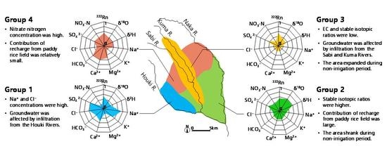
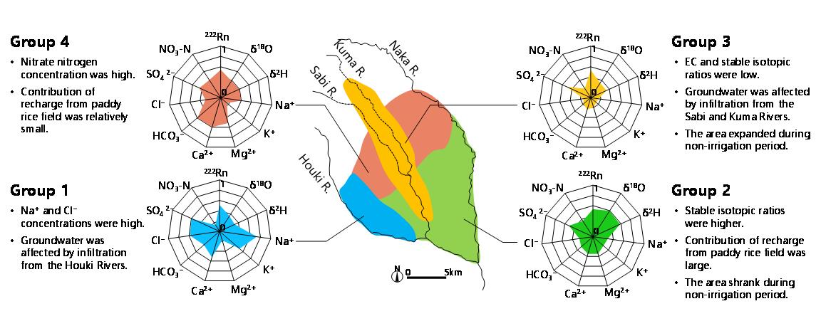
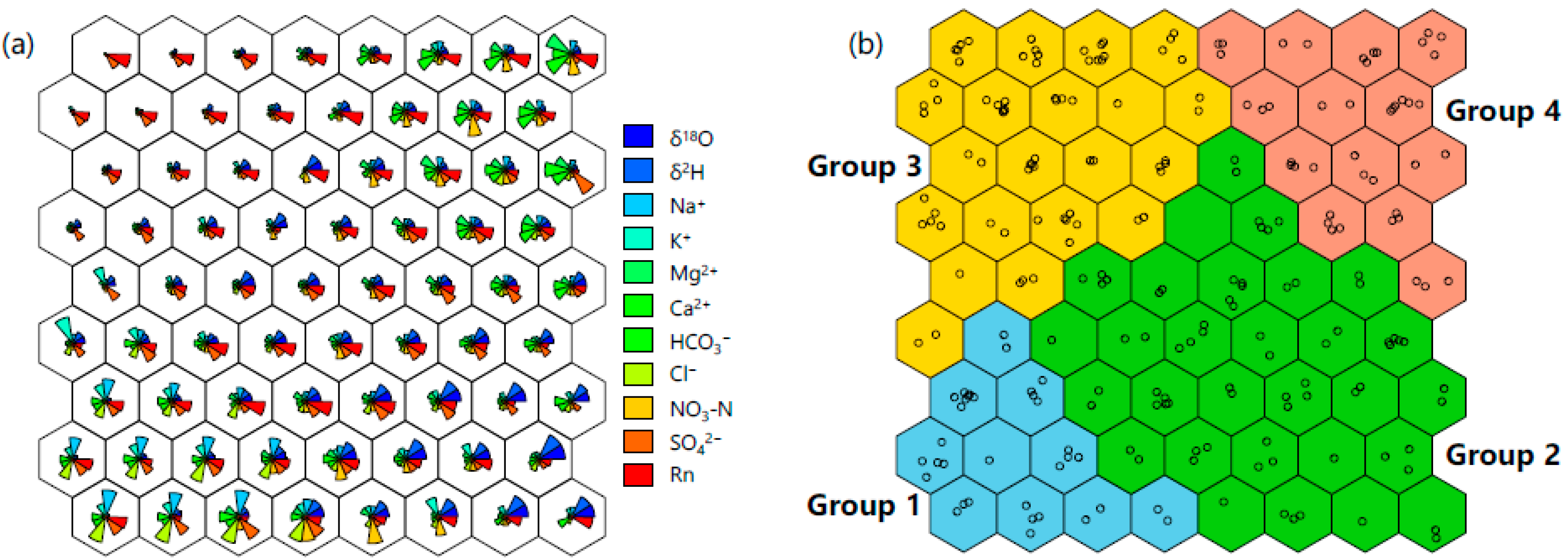
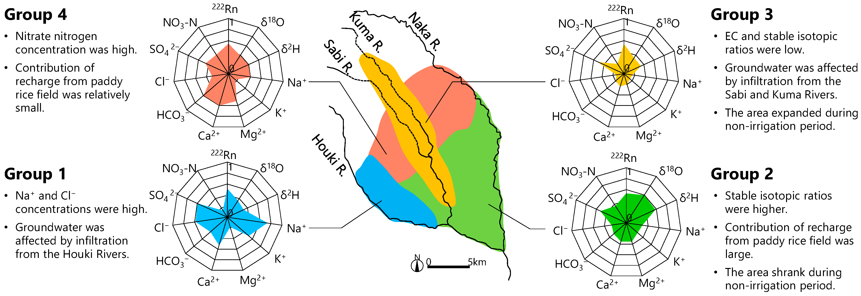
  • Group 1 groundwater, distributed around the Houki River, which flows along the western edge of the fan, had relatively low isotopic ratios, but high EC values and high Na+ and Cl concentrations. Group 1 groundwater was thus inferred to have been greatly affected by infiltration from the Houki River, which had water of a different chemical composition compared to the other rivers.
  • Group 2 groundwater, distributed in the central and lower part of the fan, had high isotopic ratios and was inferred to be recharged mainly by infiltration of paddy waters that had been affected by evaporative isotopic enrichment. However, the area of group 2 shrank during the non-irrigation period when the infiltration of paddy water did not occur.
  • Group 3 groundwater, distributed around the Sabi and Kuma Rivers, which flows down the center of the fan, had a low EC and low isotopic ratios, indicating a greater influence of infiltration of water from the two rivers compared to other recharge sources.
  • Group 4 groundwater, distributed on the upstream side of group 2 groundwater, had lower isotopic ratios than group 2 groundwater. In the upper part of the fan, few paddy rice fields but many livestock farms are distributed throughout this region; thus, recharge from paddy rice fields was relatively small. Furthermore, NO3-N concentrations in group 4 groundwaters were higher than those in the other groups.
These results show that multiple tracers could be effectively used to evaluate the influence of different groundwater recharge sources, including paddy water in rice cultivation areas, and the application of an SOM can provide understandable and readily visualized results to assist in the interpretation of the characteristics of groundwater in the fan. The findings of this study can therefore contribute to proper planning for regional groundwater use and the preservation of spring waters in the fan.

Author Contributions

Design of the study framework, T.T. and S.I.; director of the field survey and analysis T.T.; water sample collection, all authors; writing, T.T.; reviewing and editing, K.S., S.I., and S.Y. All authors have read and agreed to the published version of the manuscript.

Funding

This study was partly supported by JSPS KAKENHI (grant number JP19K06301).

Acknowledgments

We express our gratitude to the Union Nasunogahara Land Improvement District (LID: farmers’ water management organization), other LIDs, and the individual well owners for permission to sample groundwater for this study. Finally, we would like to thank the academic editors and four anonymous reviewers for their helpful comments and suggestions.

Conflicts of Interest

The authors declare no conflict of interest.

References

  1. Seto, R. Land use by landform classification in Japan -Analysis with the data of grid square basis-. Map 1986, 24, 1–11, (In Japanese with English abstract). [Google Scholar]
  2. Tabayashi, A. Irrigation systems in Japan. Geogr. Rev. Jpn. 1987, 60, 41–65. [Google Scholar] [CrossRef] [Green Version]
  3. Li, F.; Pan, G.; Tang, C.; Zhang, Q.; Yu, J. Recharge source and hydrogeochemical evolution of shallow groundwater in a complex alluvial fan system, southwest of north China plain. Environ. Geol. 2008, 55, 1109–1122. [Google Scholar] [CrossRef]
  4. Yu, H.L.; Chu, H.J. Understanding space-time patterns of groundwater system by empirical orthogonal functions: A case study in the Choshui River alluvial fan, Taiwan. J. Hydrol. 2010, 381, 239–247. [Google Scholar] [CrossRef]
  5. Eastoe, C.J.; Hutchison, W.R.; Hibbs, B.J.; Hawley, J.; Hogan, J.F. Interaction of a river with an alluvial basin aquifer: Stable isotopes, salinity and water budgets. J. Hydrol. 2010, 395, 67–78. [Google Scholar] [CrossRef]
  6. Bourke, S.A.; Cook, P.G.; Shanafield, M.; Dogramaci, S.; Clark, J.F. Characterisation of hyporheic exchange in a losing stream using radon-222. J. Hydrol. 2014, 519, 94–105. [Google Scholar] [CrossRef] [Green Version]
  7. Karan, S.; Sebok, E.; Engesgaard, P. Air/water/sediment temperature contrasts in small streams to identify groundwater seepage locations. Hydrol. Process. 2017, 31, 1258–1270. [Google Scholar] [CrossRef]
  8. Yoshioka, Y.; Nakamura, K.; Nakano, T.; Horino, H.; Shin, K.C.; Hashimoto, S.; Kawashima, S. Multiple-indicator study of groundwater flow and chemistry and the impacts of river and paddy water on groundwater in the alluvial fan of the Tedori River, Japan. Hydrol. Process. 2016, 30, 2804–2816. [Google Scholar] [CrossRef]
  9. Doveri, M.; Mussi, M. Water isotopes as environmental tracers for conceptual understanding of groundwater flow: An application for fractured aquifer systems in the “Scansano-Magliano in Toscana” area (Southern Tuscany, Italy). Water 2014, 6, 2255–2277. [Google Scholar] [CrossRef] [Green Version]
  10. Yeh, H.F.; Lin, H.I.; Lee, C.H.; Hsu, K.C.; Wu, C.S. Identifying seasonal groundwater recharge using environmental stable isotopes. Water 2014, 6, 2849–2861. [Google Scholar] [CrossRef]
  11. Zhong, C.H.; Yang, Q.C.; Ma, H.Y.; Bian, J.M.; Zhang, S.H.; Lu, X.G. Application of environmental isotopes to identify recharge source, age, and renewability of phreatic water in Yinchuan Basin. Hydrol. Process. 2019, 33, 2166–2173. [Google Scholar] [CrossRef]
  12. Liu, Y.; Yamanaka, T. Tracing groundwater recharge sources in a mountain-plain transitional area using stable isotopes and hydrochemistry. J. Hydrol. 2012, 464, 116–126. [Google Scholar] [CrossRef] [Green Version]
  13. Valder, J.F.; Long, A.J.; Davis, A.D.; Kenner, S.J. Multivariate statistical approach to estimate mixing proportions for unknown end members. J. Hydrol. 2012, 460–461, 65–76. [Google Scholar] [CrossRef]
  14. Cortes, J.E.; Muñoz, L.F.; Gonzalez, C.A.; Niño, J.E.; Polo, A.; Suspes, A.; Siachoque, S.C.; Hernãndez, A.; Trujillo, H. Hydrogeochemistry of the formation waters in the San Francisco field, UMV basin, Colombia—A multivariate statistical approach. J. Hydrol. 2016, 539, 113–124. [Google Scholar] [CrossRef]
  15. Islam, M.M.; Lenz, O.K.; Azad, A.K.; Ara, M.H.; Rahman, M.; Hassan, N. Assessment of spatio-temporal variations in water quality of Shailmari River, Khulna (Bangladesh) using multivariate statistical techniques. J. Geosci. Environ. Protect. 2017, 5, 1–26. [Google Scholar] [CrossRef]
  16. Dieng, N.M.; Orban, P.; Stumpp, C.; Faye, S.; Dassargues, A. Temporal changes in groundwater quality of the Saloum coastal aquifer. J. Hydrol. Reg. Stud. 2017, 9, 163–182. [Google Scholar] [CrossRef]
  17. Chen, I.T.; Chang, L.C.; Chang, F.J. Exploring the spatio-temporal interrelation between groundwater and surface water by using the self-organizing maps. J. Hydrol. 2018, 556, 131–142. [Google Scholar] [CrossRef]
  18. Choi, B.Y.; Yun, S.T.; Kim, K.H.; Kim, J.W.; Kim, H.M.; Koh, Y.K. Hydrogeochemical interpretation of South Korean groundwater monitoring data using Self-Organizing Maps. J. Geochem. Explor. 2014, 137, 73–84. [Google Scholar] [CrossRef]
  19. Nakagawa, K.; Amano, H.; Kawamura, A.; Berndtsson, R. Classification of groundwater chemistry in Shimabara, using self-organizing maps. Hydrol. Res. 2017, 48, 840–850. [Google Scholar] [CrossRef] [Green Version]
  20. Agoubi, B. Assessing hydrothermal groundwater flow path using Kohonen’s SOM geochemical data and groundwater temperature cooling trend. Environ. Sci. Pollut. Res. 2018, 25, 13597–13610. [Google Scholar] [CrossRef]
  21. An, Y.; Zou, Z.; Li, R. Descriptive Characteristics of Surface Water Quality in Hong Kong by a Self-Organising Map. Int. J. Environ. Res. Public Health 2016, 13, 115. [Google Scholar] [CrossRef] [PubMed]
  22. Rural Development Bureau, Ministry of Agriculture, Forestry and Fisheries (MAFF). Actual Use of Groundwater for Agriculture; MAFF: Tokyo, Japan, 2011; pp. 1–13. (In Japanese) [Google Scholar]
  23. Otawara City Habitat of Three-Spined Stickleback (Taya River). Available online: https://www.city.ohtawara.tochigi.jp/docs/2013082781284/ (accessed on 28 October 2019). (In Japanese).
  24. Wakui, H.; Yamanaka, T. Source of groundwater recharge and their local differences in the central part of Nasu fan as revealed by stable isotopes. J. Groundw. Hydrol. 2006, 48, 263–277, (In Japanese with English abstract). [Google Scholar] [CrossRef]
  25. Hiyama, T.; Suzuki, Y. Groundwater in the Nasuno basin -Spatial and seasonal changes in water quality-. J. Jpn. Assoc. Hydrol. Sci. 1991, 21, 143–154, (In Japanese with English abstract). [Google Scholar]
  26. Babiker, I.S.; Mohamed, M.A.A.; Hiyama, T. Assessing groundwater quality using GIS. Water Resour. Manag. 2007, 21, 699–715. [Google Scholar] [CrossRef]
  27. Somura, H.; Goto, A.; Matsui, H.; Elhassan, A.M. Impacts of nutrient management and decrease in paddy field area on groundwater nitrate concentration: A case study at the Nasunogahara alluvial fan, Tochigi Prefecture, Japan. Hydrol. Process. 2008, 22, 4752–4766. [Google Scholar] [CrossRef]
  28. Elhassan, A.M.; Goto, A.; Mizutani, M. Combining a tank model with a groundwater model for simulating regional groundwater flow in an alluvial fan. Trans. Jpn. Soc. Irrig. 2001, 215, 21–29. [Google Scholar]
  29. National Land Information Division, National Spatial Planning and Regional Policy Bureau, MILT of Japan. National Land Numerical Information Download Service. Available online: http://nlftp.mlit.go.jp/ksj/ (accessed on 4 September 2019).
  30. Geospatial Information Authority of Japan. GSI Map. Available online: https://maps.gsi.go.jp/ (accessed on 4 September 2019).
  31. Hydrogeological Map of Nasuno-ga-hara Area. Kanto Regional Agricultural Administration Office; MAFF of Japan: Tokyo, Japan, 1993. (In Japanese)
  32. The Survey Report of Subsurface Dam in Kanto Area. Kanto Regional Agricultural Administration Office; MAFF of Japan: Tokyo, Japan, 1999. (In Japanese)
  33. IAEA/GNIP Precipitation Sampling Guide (V2.02). September 2014. Available online: http://www-naweb.iaea.org/napc/ih/documents/other/gnip_manual_v2.02_en_hq.pdf (accessed on 31 October 2019).
  34. Hoehn, E.; von Gunten, H.R. Radon in groundwater: A tool to assess infiltration from surface waters to aquifers. Water Resour. Res. 1989, 25, 1795–1803. [Google Scholar] [CrossRef] [Green Version]
  35. Hamada, H. Estimation of groundwater flow rate using the decay of 222Rn in a well. J. Environ. Radioact. 2000, 47, 1–13. [Google Scholar] [CrossRef]
  36. Hamada, H.; Komae, T. Investigation on shallow groundwater in a small basin using natural radioisotopes. Radioisotopes 1996, 45, 71–81. [Google Scholar] [CrossRef] [Green Version]
  37. Gat, J.R. Oxygen and hydrogen isotopes in the hydrologic cycle. Annu. Rev. Earth Planet. Sci. 1996, 24, 225–262. [Google Scholar] [CrossRef] [Green Version]
  38. Dansgaard, W. Stable isotopes in precipitation. Tellus 1964, 16, 436–468. [Google Scholar] [CrossRef]
  39. Kohonen, T. Self-organized formation of topologically correct feature maps. Biol. Cybern. 1982, 43, 59–69. [Google Scholar] [CrossRef]
  40. Jin, Y.H.; Kawamura, A.; Park, S.C.; Nakagawa, N.; Amaguchi, H.; Olsson, J. Spatiotemporal classification of environmental monitoring data in the Yeongsan River basin, Korea, using self-organizing maps. J. Environ. Monit. 2011, 13, 2886–2894. [Google Scholar] [CrossRef] [PubMed]
  41. Nguyen, T.T.; Kawamura, A.; Tong, T.N.; Nakagawa, N.; Amaguchi, H.; Gilbuena, R. Clustering spatio–seasonal hydrogeochemical data using self-organizing maps for groundwater quality assessment in the Red River Delta. J. Hydrol. 2015, 522, 661–673. [Google Scholar] [CrossRef]
  42. Farsadnia, F.; Rostami Kamrood, M.; Moghaddam Nia, A.; Modarres, R.; Bray, M.T.; Han, D.; Sadatinejad, J. Identification of homogeneous regions for regionalization of watersheds by two-level self-organizing feature maps. J. Hydrol. 2014, 509, 387–397. [Google Scholar] [CrossRef]
  43. Hentati, A.; Kawamura, A.; Amaguchi, H.; Iseri, Y. Evaluation of sedimentation vulnerability at small hillside reservoirs in the semi-arid region of Tunisia using the Self-Organizing Map. Geomorphology 2010, 122, 56–64. [Google Scholar] [CrossRef]
  44. Vesanto, J.; Alhoniemi, R. Clustering of the self organizing map. IEEE Trans. Neural Netw. 2000, 11, 586–600. [Google Scholar] [CrossRef]
  45. Faggiano, L.; Zwart, D.; García-Berthou, E.; Lek, S.; Gevrey, M. Patterning ecological risk of pesticide contamination at the river basin scale. Sci. Total Environ. 2010, 408, 2319–2326. [Google Scholar] [CrossRef]
  46. Wehrens, R.; Buydens, L.M.C. Self-and super-organizing maps in r: The kohonen package. J. Stat. Softw. 2017, 21, 1–19. [Google Scholar]
  47. Ogawa, R.; Yamanaka, M. Hydrogeochemical controlling on groundwater in the Hadano Basin, Kanagawa Prefecture: Processes of mineral weathering and dissolved inorganic carbon supply. In Proceedings of the Institute of Natural Sciences. Sect; Nihon University: Tokyo, Japan, 2018; Volume 53, pp. 125–134, (In Japanese with English abstract). [Google Scholar]
  48. Yamanaka, T.; Tanaka, T.; Asanuma, J.; Hamada, Y. Interaction Between Groundwater and River Water in the Nasu Fan, Tochigi; Bull Terr Environment Research Ctr., University of Tsukuba: Tsukuba, Japan, 2003; Volume 4, pp. 51–59, (In Japanese with English abstract). [Google Scholar]
  49. Craig, H. Isotopic variations in meteoric waters. Science 1961, 133, 1702–1703. [Google Scholar] [CrossRef]
  50. Ichiyanagi, K.; Tanoue, M. Spatial analysis of annual mean stable isotopes in precipitation across Japan based on an intensive observation period throughout 2013. Istopes Environ. Health Stud. 2016, 52, 353–362. [Google Scholar] [CrossRef] [PubMed]
  51. Yoshimura, K.; Ichiyanagi, K. A reconsideration of seasonal variation in precipitation deuterium excess over East Asia. J. Jpn. Soc. Hydrol. Water Res. 2009, 22, 262–276, (In Japanese with English abstract). [Google Scholar] [CrossRef] [Green Version]
  52. Gibson, J.J.; Prepas, E.E.; McEachern, P. Quantitative comparison of lake throughflow, residency, and catchment runoff using stable isotopes: Modelling and results from a regional survey of Boreal lakes. J. Hydrol. 2002, 262, 128–144. [Google Scholar] [CrossRef]
  53. Tsuchihara, T.; Shirahata, K.; Yoshimoto, S.; Ishida, S. National-scale variations in the stable isotopic compositions of irrigation-pond and spring waters across Japan. Paddy Water Environ. 2019, 17, 429–438. [Google Scholar] [CrossRef]
  54. Mahindawansha, A.; Breuer, L.; Chamorro, A.; Kraft, P. High-frequency water isotopic analysis using an automatic water sampling system in rice-based cropping systems. Water 2018, 10, 1327. [Google Scholar] [CrossRef] [Green Version]
  55. Hamada, H.; Komae, T. Analysis of recharge by paddy field irrigation using 222Rn concentration in groundwater as an indicator. J. Hydrol. 1998, 205, 92–100. [Google Scholar] [CrossRef]
Figure 1. Maps showing the (a) location of the study site, (b) land use, and (c) water sampling sites. Groundwater was not sampled at the sites denoted by white circles in March 2019 because the wells were dry owing to a drop in the groundwater level. The land use map was created by using National Land Numerical Information [29]. The gray topographic base map in (c) was from the Geospatial Information Authority of Japan [30].
Water 12 00278 g001
Figure 2. Geological cross section of the Nasunogahara alluvial fan (modified from the Kanto Regional Agricultural Administration Office [31]).
Water 12 00278 g002
Figure 3. (a) Spatial distribution of the groundwater level in the irrigation period (IP), (b) depth to the water table in the IP, and (c) cross-sections of the groundwater table. The contour line of the ground surface was modified from the Geospatial Information Authority of Japan [30].
Water 12 00278 g003
Figure 4. Trilinear diagram of groundwater, spring water, river water, and paddy water.
Water 12 00278 g004
Figure 5. Hexa-diagrams of groundwater, spring water, river water, and paddy water.
Water 12 00278 g005
Figure 6. Relationships between EC, Ca2+, and HCO3 with groundwater level.
Water 12 00278 g006
Figure 7. Distributions of (a) EC, (b) Ca2+, (c) SO42−, and (d) Cl concentrations in the groundwater. The upper and lower maps show the data in the IP and NP, respectively.
Water 12 00278 g007
Figure 8. Relationship between δ18O and δ2H of (a) rainwater and paddy water and (b) groundwater. LMWL is the local meteoric water line identified by fitting a regression line to observations at sites P1 and P2. PWRL is the regression line fitted to the paddy water data.
Water 12 00278 g008
Figure 9. Distributions of (a) δ18O, (b) d-excess, and (c) the 222Rn concentration in groundwater in the IP (upper maps) and NP (lower maps).
Water 12 00278 g009
Figure 10. Component planes of the isotopic and hydrochemical parameters: (a) δ18O, (b) δ2H, (c) Na+, (d) K+, (e) Mg2+, (f) Ca2+, (g) HCO3, (h) Cl, (i) NO3-N, (j) SO42−, and (k) 222Rn. Each plane shows the standardized value of each parameter (transformed to the range from 0 to 1) in each node.
Water 12 00278 g010
Figure 11. (a) All reference vectors in each of the 72 nodes and (b) classification of the self-organizing map (SOM) nodes into four groups. The circles on each map hexagon represent the groundwater samples assigned to that node.
Water 12 00278 g011
Figure 12. Spatial distribution of hexa-diagrams of groundwaters in four groups classified by the SOM in the (a) IP and (b) NP.
Water 12 00278 g012
Figure 13. Trilinear diagram of the four groundwater groups.
Water 12 00278 g013
Figure 14. Relationship between δ18O and δ2H of the four groundwater groups. LMWL and PWRL are the local meteoric water line and the paddy water regression line, respectively, as shown in Figure 8.
Water 12 00278 g014
Figure 15. Characteristics of the Nasunogahara alluvial fan groundwaters in each of the four groups. Medians of all variables plotted on the radar charts were transformed to range from 0 to 1.
Water 12 00278 g015
Figure 16. Comparison of groundwater EC values and isotopic compositions between the IP and NP at observation sites classified into group 2 in the IP.
Water 12 00278 g016
Table 1. Analytical results for groundwater, spring water, paddy water, river water, and rainwater.
TypeGroup/SitenPeriod ECNa+K+Mg2+Ca2+HCO3ClSO42−NO3-Nδ18Oδ2Hd-Excess222Rn
mS/mmg/Lmg/Lmg/Lmg/Lmg/Lmg/Lmg/Lmg/LBq/L
GroundwaterAll222IP, NPMean17.39.00.31.34.942.08.720.12.6−8.5−5612.512.4
Median17.48.60.31.24.640.38.120.72.5−8.6−5612.612.9
25th15.17.10.20.93.930.46.118.21.9−8.9−5711.410.7
75th19.710.10.31.65.850.810.222.83.1−8.2−5413.414.5
Group 134IP, NPMean20.313.92.04.116.846.415.424.01.9−8.8−5712.911.6
Median20.013.82.13.816.446.915.423.51.6−8.8−5713.012.4
25th19.513.31.93.615.844.413.822.81.2−9.1−5912.410.1
75th20.615.12.34.117.550.316.524.42.0−8.6−5613.313.5
Group 273IP, NPMean17.28.61.45.113.539.08.620.23.0−8.0−5311.012.5
Median17.08.51.45.213.038.48.120.63.0−8.1−5411.112.9
25th16.27.61.14.612.133.67.118.62.6−8.3−5510.210.6
75th18.09.11.55.714.645.29.823.53.4−7.7−5211.814.6
Group 372IP, NPMean14.46.81.13.910.729.65.519.22.1−8.8−5713.512.2
Median14.06.71.03.910.828.95.220.42.0−8.8−5713.512.9
25th13.26.10.73.59.724.94.318.31.7−9.1−5812.810.4
75th15.27.31.44.211.733.76.421.32.3−8.6−5614.515.0
Group 443IP, NPMean20.09.71.06.718.264.49.118.33.4−8.6−5612.913.2
Median20.09.81.06.617.862.88.918.53.2−8.7−5612.913.0
25th19.39.20.86.016.456.38.315.82.8−8.8−5712.311.2
75th21.210.31.27.119.869.79.820.74.0−8.4−5513.414.8
Spring waterSP11IP11.85.30.62.89.019.43.619.11.4−9.4−6015.113.3
SP21IP11.35.30.72.89.524.43.820.91.5−9.3−6014.38.4
SP31IP13.65.90.83.410.522.05.121.01.9−9.0−5813.811.3
SP42IP, NPMean14.17.71.24.011.536.94.918.91.9−8.9−5713.711.7
SP52IP, NPMean14.47.91.14.311.031.76.019.12.2−8.8−5713.412.6
SP62IP, NPMean18.412.22.03.716.442.613.123.81.9−8.9−5813.113.3
Paddy water14IPMean11.76.23.32.97.119.16.920.50.5−5.4−45−2.2
River waterNaka R.2IP, NPMean15.710.20.21.615.925.32.742.70.1−10.0−6317.30.3
Kuma R.2IP, NPMean14.85.00.22.017.69.61.052.50.2−9.9−6216.40.2
Sabi R.2IP, NPMean11.13.60.42.510.611.91.232.50.2−9.7−6215.40.5
Houki R.2IP, NPMean23.223.32.82.814.947.523.927.50.3−10.0−6415.80.3
RainwaterP116All yearMean−8.5−5612.1
P212All yearMean−8.0−5212.1
EC: electrical conductivity, IP: irrigation period, NP: non-irrigation period, –: not analyzed, 25th and 75th: 25th and 75th percentiles, mean values of rainwater were weighted using the precipitation amount.
Table 2. Pearson correlation coefficients for EC and major ions of all groundwater samples.
ECNa+K+Mg2+Ca2+HCO3ClSO42−NO3-N
EC1
Na+0.671
K+0.240.451
Mg2+0.520.19−0.191
Ca2+0.820.600.190.561
HCO30.670.500.020.700.841
Cl0.660.910.540.150.610.421
SO42−0.310.290.19−0.010.26−0.130.231
NO3-N0.320.01−0.070.690.270.280.08−0.181

