Climate Change Impacts on Reservoir Inflow in the Prairie Pothole Region: A Watershed Model Analysis


1
Department of Civil Engineering, University of Manitoba, Winnipeg, MB R3T 5V6, Canada
2
Department of Food, Agricultural and Biological Engineering, The Ohio State University, 590 Woody Hayes Dr, Columbus, OH 43210, USA
3
Hydrologic Forecasting & Coordination, Manitoba Infrastructure, 2nd Floor-280 Broadway, Winnipeg, MB R3C 0R8, Canada
4
Department of Geography, University of Calgary, ESB 458, 2500 University Dr NW, Calgary, AB T2N 1N4, Canada
*
Author to whom correspondence should be addressed.
Water 2020, 12(1), 271; https://doi.org/10.3390/w12010271
Submission received: 6 December 2019
/
Revised: 6 January 2020
/
Accepted: 15 January 2020
/
Published: 17 January 2020
(This article belongs to the Special Issue Effects of Climate Change on Water Resources)
Abstract
:The Prairie Pothole Region (PPR) is known for its hydrologically complex landscape with a large number of pothole wetlands. However, most watershed-scale hydrologic models that are applied in this region are incapable of representing the dynamic nature of contributing area and fill-spill processes affected by pothole wetlands. The inability to simulate these processes represents a critical limitation for operators and flood forecasters and may hinder the management of large reservoirs. We used a modified version of the soil water assessment tool (SWAT) model capable of simulating the dynamics of variable contributing areas and fill-spill processes to assess the impact of climate change on upstream inflows into the Shellmouth reservoir (also called Lake of the Prairie), which is an important reservoir built to provide multiple purposes, including flood and drought mitigation. We calibrated our modified SWAT model at a daily time step using SUFI-2 algorithm within SWAT-CUP for the period 1991–2000 and validated for 2005–2014, which gave acceptable performance statistics for both the calibration (KGE = 0.70, PBIAS = −13.5) and validation (KGE = 0.70, PBIAS = 21.5) periods. We then forced the calibrated model with future climate projections using representative concentration pathways (RCPs; 4.5, 8.5) for the near (2011–2040) and middle futures (2041–2070) of multiple regional climate models (RCMs). Our modeling results suggest that climate change will lead to a two-fold increase in winter streamflow, a slight increase in summer flow, and decrease spring peak flows into the Shellmouth reservoir. Investigating the impact of climate change on the operation of the Shellmouth reservoir is critically important because climate change could present significant challenges to the operation and management of the reservoir.
1. Introduction
Climate change is predicted to significantly impact the availability of water resources around the world [1]. Scientific consensus is that increasing temperature will alter both the quantity and timing of regional precipitation, evapotranspiration, and soil moisture, which will in-turn affect hydrologic flows into lakes and streams [2,3,4,5]. Climate change is also predicted to increase precipitation intensity, which could lead to higher rates of surface runoff causing an increased risk of floods. Increasing temperature will enhance evapotranspiration rate, which may increase the demand for water availability during the peak growing season [3,6]. With more than one-sixth of the earth population relying on glaciers and seasonal snowpacks for their water supply, the consequences of climate change and interrelated hydrological changes for future water availability are likely to be severe [7]. In order to better tackle these future water resource management issues, the impact of climate change on components of the water balance must be quantified from regional to local scales [8].
Based on numerous studies, climate change over the Prairie Pothole Region (PPR) of North America, which spans across Alberta, Saskatchewan, and Manitoba in Canada and extends into North Dakota, South Dakota, Iowa, Minnesota, and Montana in the United States, will significantly impact runoff that is driven by seasonal snowmelt [3,9,10,11,12,13]. The Canadian portion of the Prairie region, especially the central part, is projected to warm over the next 60 years [3,14], which may result in excessive moisture risk [15] and frequent drought conditions. The latest report from Environment and Climate Change Canada (ECCC) projected a 6.5 °C rise in temperature for the Canadian Prairies [16]. In the PPR, winter snowfall accounts for 30% of total annual precipitation yet is responsible for approximately 80% to the total annual surface runoff. Climate change may disturb the seasonality and amount of precipitation and air temperature causing significant impact on the distribution, volume and timing of snowfall, which in turn will alter the hydrology of the prairies.
Few past studies have evaluated the impact of climate change on the hydrology of the Canadian Prairie region. For example, Canadian Regional Climate Model (CRCM) ver. 5 was utilized [3] to assess impacts of climate and land use change on the hydrology of the Upper Assiniboine River basin. While the study outlined that climate will play far more significant role in changing hydrologic regime of the watershed in comparison to the land use changes, the study’s primary recommendation focused on the use of multiple climate models to conduct similar studies to come into a comprehensive recommendation. The soil water assessment tool (SWAT) hydrologic model was used to assess climate-induced changes in hydrologic and nutrient fluxes in the Upper Assiniboine watershed [17]. Results of the study revealed clear evidence of changes in the distribution of snowmelt and runoff regimes. Uncertainties in hydrologic responses to climate changes [18] was assessed in the Assiniboia watershed that lies in the Canadian portion of the PPR. The study revealed that uncertainties in hydrologic responses are mainly due to the choice of RCM and downscaling techniques and that result of any climate change study based on only one RCM should be interpreted with caution. In a different study [19], a weighted multi-RCM ensemble and stochastic weather generator is used to generate future climate change projections for the Assiniboia watershed in Canada. It was noted that using ensemble reduces biases in both precipitation and temperature.
Several other studies highlighted how climate change would impact the distribution of water availability in the Prairie region. For example, while evaluating the impact of climate change on the Smith Creek Research Basin, it was noted that climate change has brought gradual increases in rainfall, an earlier snowmelt by 2 weeks, and a 50% increase in the multiple -day rainfall events [20]. In a different study [21], it was indicated that impact of climate change will likely cause a 26% difference in the availability of water resources including significant shifts in the intensity, duration, and frequency of precipitation events over the Qu’Appelle watershed that lies within the Canadian prairie region. Other studies such as those by [22,23,24,25] suggested an earlier snowmelt due to increasing temperature which may then affect an earlier spring peak runoff and drier late summer.
Previous studies serve as an important guide to our understanding regarding climate change impacts on hydrological processes within the PPR. Hydrological model constructed to assess hydrology of the Prairie region must pay close attention to the important role that pothole wetlands play in the hydrology of the prairie region. Pothole wetlands also known as geographically isolated wetlands (GIWs) are wetlands that do not have any apparent surface water connections with the stream network. Based on several studies [26,27,28,29], it is well documented that surface runoff in the prairie region often drains into these pothole wetlands, retaining water for longer time periods while not necessarily contributing flow to the stream under normal conditions. However, during times of high runoff, these depressions fill to capacity and spill, to other downgradient wetlands or to the stream. Hence, temporary hydrologic connections can form which result in dynamic increases in the contributing area within the watershed [30].
A modified version of the SWAT model was constructed to better represent pothole wetlands and their impact on watershed hydrology [31,32,33]. Though the modification addressed some of the Prairie region modeling limitations, it imposed significant and sometimes prohibitive computational challenges [34]. Such limitations are particularly important in the context of climate change analyses, for which models are commonly executed over longer time periods. Thus, there is a pressing need to address both climate change impact assessment and model computational challenges while using the enhanced representation of pothole wetlands.
In this study, we utilized a new concept of pothole wetland representation based on pothole wetlands storage capacity, which significantly reduced model computational demand. We then constructed a series of climate change scenarios to assess future water resource availability in the Upper Assiniboine River Basin (UARB) with the goal of quantifying the impact of climate change on reservoir inflow. The UARB is a headwater catchment to the Shellmouth reservoir, also known as the ‘Lake of the Prairie’, which is an important reservoir that provides multiple functions including flood control, water supply, irrigation, and recreation. This study is of critical importance for the Hydrologic Forecast Centre of Manitoba (HFC-MI), which has a mandate of managing and operating the Shellmouth reservoir, in understanding the effect of climate change in the future inflow trends into the reservoir and the associated operational challenges.
2. Materials and Methods
2.1. The Shellmouth Reservoir Watershed
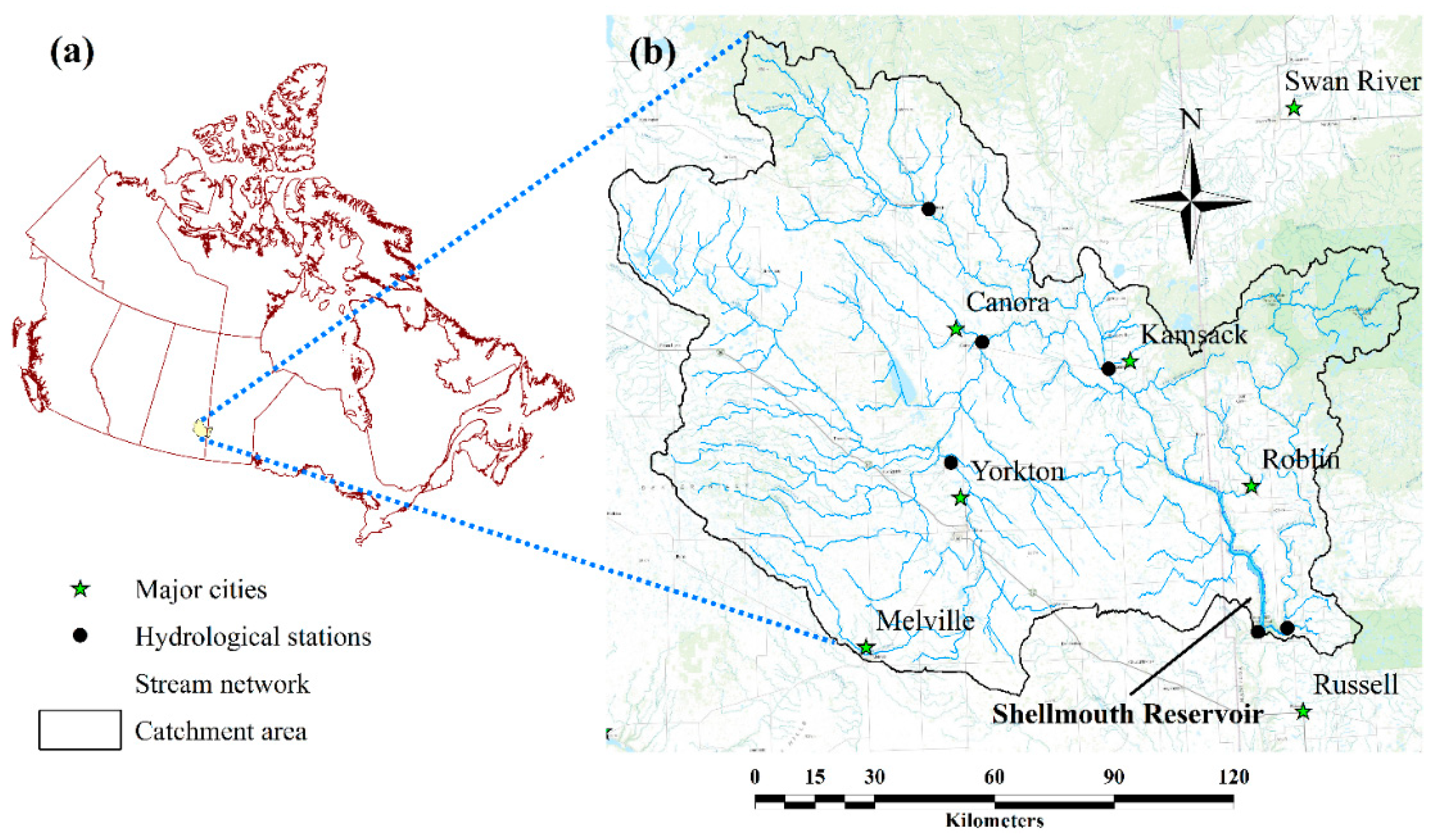
The Shellmouth reservoir is located within the Upper Assiniboine River Basin (UARB) catchment, which spans across the provinces of Manitoba and Saskatchewan in Canada (Figure 1). Total watershed area of the UARB is 18,000 km2 and is known for its hydrologically complex landscape due the presence of a large number of pothole wetlands.
The Shellmouth dam is a multipurpose, earth-filled embankment dam, constructed in 1972 by the Prairie Farm Rehabilitation Administration (PFRA) in a deep, wide portion of the Assiniboine River valley. The dam is 21 m high and 64 m wide. The storage capacity of the dam is 480 × 106 m3 at spillway crest (429.3 m above mean sea level, masl). The surface area of the dam at full reservoir capacity is 6151 m2. The dam and reservoir were part of a strategy to reduce the risk of flooding on the Assiniboine River and in Winnipeg city, while providing water supply and irrigation benefits to downstream residents. For more details, the readers are referred to the Hydrologic Forecasting Centre website (https://www.gov.mb.ca/mit/wms/shellmouth/index.html) where a complete description, benefit and services of the dam is provided.
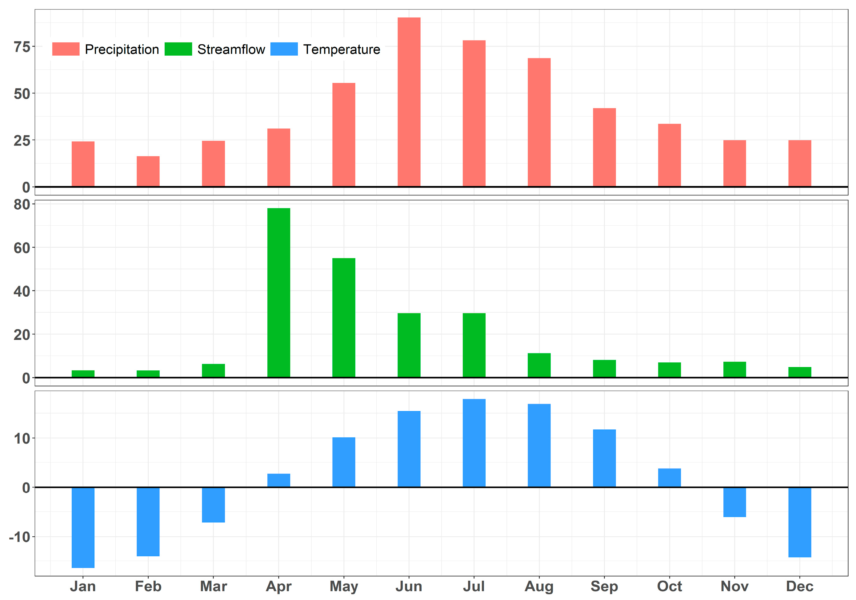
The climate of UARB is continental sub-humid characterized by long cold winters and a short summer [3,9]. Mean annual precipitation is 510 mm and mean annual temperature is 1.5 °C during the periods 1988–2017. Approximately 26% of the watershed’s precipitation falls as snow, which melts during spring. Snowmelt accounts for 82% of total mean annual streamflow [17] (Figure 2). Agriculture is the dominant land use, which covers 70% of the watershed area followed by forest (17%) and grassland (6.5%) [35]. Wetlands covers 2.5% of the total watershed area (525 km2). Most of the watershed area is level with an average elevation of 577 masl. The lowest point is 388 masl, which is located in Shellmouth reservoir while the highest point, which is 788 masl, is located in the upland of the UARB. Approximately 70% of the UARB is characterized by black chernozemic soils that are high in organic matter and developed under native grassland vegetation [36].
2.2. Hydrological Model
We used a modified version of the SWAT hydrologic model to assess the impact of climate change on the operation of the Shellmouth reservoir based on projection of upstream inflows. SWAT is a continuous processes-based and semi-distributed model [37]. The model partitions the watershed into a series of sub-basins, which are further sub-divided into hydrologic response units (HRUs). HRUs are the smallest computational units in the model and are delineated as unique combinations of land use, soil type, and elevation within each sub basin. A daily hydrologic balance is simulated for each HRU that includes surface runoff, evapotranspiration, redistribution of water within soil profile, sediments yield, nutrient cycles, and return flow [38,39]. The simulated water, nutrient and sediment export from each HRU is then routed to the sub basin’s river channel and progressively downstream [37].
The modified version of the SWAT model has an enhanced representation of Prairie pothole wetlands. The modified model has been previously demonstrated to better replicate streamflow and other dominant physical processes such as the fill-spill of the prairie pothole wetlands, which are the defining characteristics of the PPR [28,32,34]. As noted in earlier studies, a limitation of the modified model was the computational cost in representing pothole wetlands at larger spatio-temporal scales [32,34]. Hence, we further modified the model to include a threshold wetland storage capacity to decrease computational cost without significantly reducing the enhanced spatial representation of pothole wetlands and model simulation accuracy. It should be noted that our goal was to more accurately predict inflows to the reservoir impacted by the prairie pothole landscape and climate change, but not to utilize SWAT to project the outflows. Hydrologic forecasters utilize their own operational models to predict outflow based on knowing the reservoir inflow.
2.3. SWAT Model Data Requirement
Soil type, topography, land use, and climate data are the basic datasets required to construct a SWAT model (Table 1). The Soil Landscapes of Canada version 3.2 (SLC ver. 3.2) was used to extract soil properties for the study watershed [40]. The 30-m resolution Land use map [35] and the 90 m digital elevation model (DEM) from the Canadian Digital Elevation Model Data (CDED) were obtained from the Canadian GeoGratis open data portal (http://geogratis.gc.ca/). HFC-MI provided climate data at a daily time step for the period 1988–2017. Environment and Climate Change Canada (ECCC) is the main source of climate data, however, HFC-MI through an agreement with Agriculture and Agri-Food Canada (AAFC) receives quality assured data, which was also used in this study. The observed daily streamflow time series, required for model calibration and validation, was obtained from Water Survey of Canada (WSC) hydrometric database (HYDAT). The HFC-MI records daily inflow to the Shellmouth reservoir, which is not provided through the HYDAT database. The daily inflow data into the reservoir was used in the calibrating and validating the model.
2.4. Experimental Setup
We used the ArcGIS-ArcSWAT interface for SWAT 2012 (rev 627) to develop the UARB model. We used a DEM [31] to delineate and discretized the UARB into 33 sub-watersheds while inserting a reservoir at the catchment outlet. Following watershed discretization, we delineated HRUs using the land use, soil type, and slope map of the area. We used a weather generator based on the HFC-MI furnished climate data to develop and imported precipitation and temperature inputs for the model. The reservoir database was updated with Shellmouth reservoir data obtained from the HFC-MI.
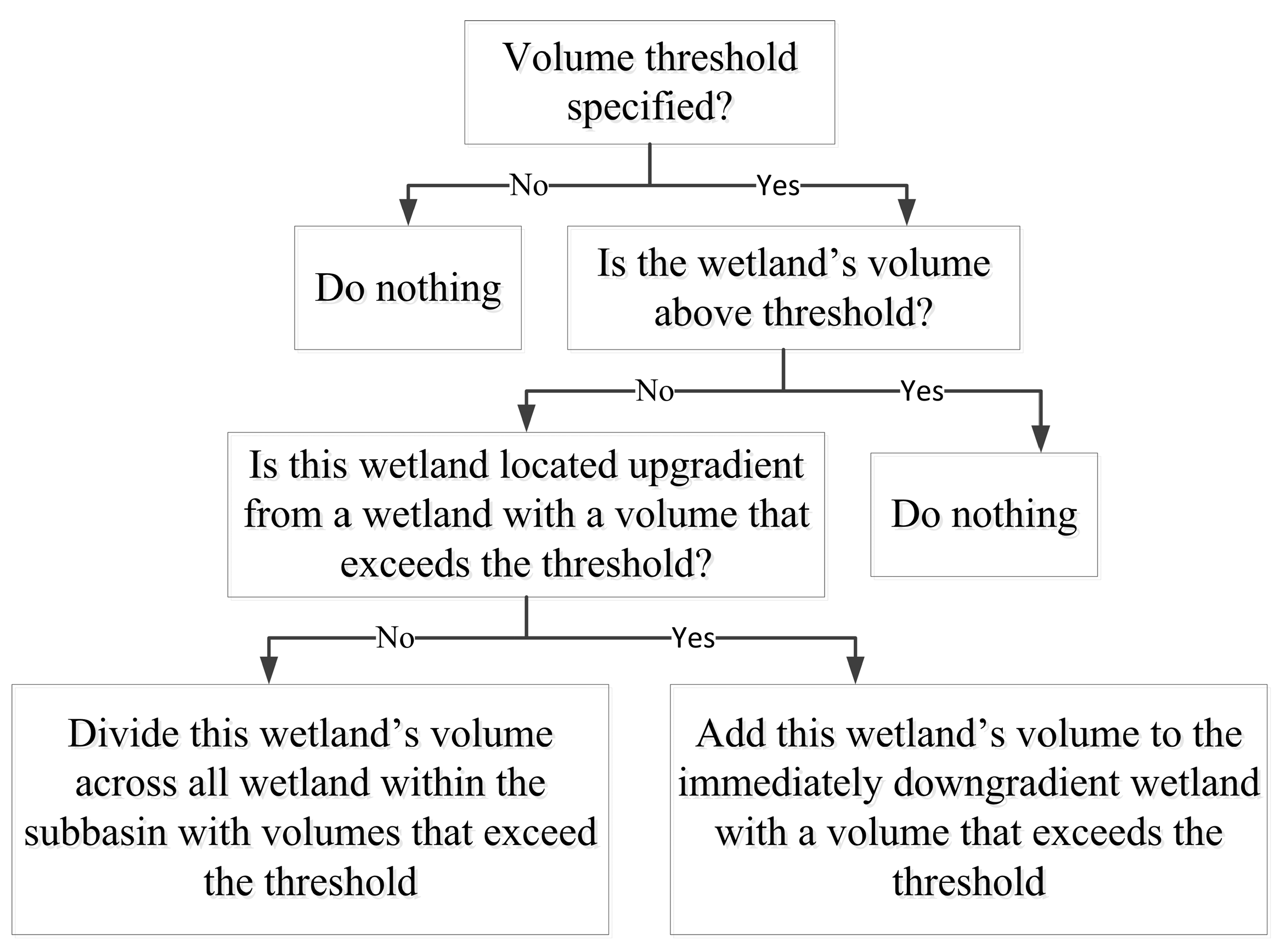
The modified SWAT model provides an improved representation of pothole fill-spill routing processes among pothole wetlands within a sub-basin [3,32]. The standard representation of pothole at HRU level was redefined following a procedure similar to [34]. The pothole modification significantly increased the number of HRUs; elevating the number from 912 in the standard version to 24,000 in the modified version. The increased number of HRUs increased model complexity, model runtime, and other computational demands. Model execution time is of critical importance in this study due to reservoir inflow forecasts and the long-term simulation of climate change impacts across multiple scenarios. Hence, we introduced a wetland storage capacity threshold to balance model accuracy with computational resource requirements (Figure 3).
We elected to use a threshold value of 50 × 103 m3, after testing several variants and finding an acceptable computational cost. Wetlands with storage capacities greater than the threshold were simulated as separate GIW-HRUs, and wetlands with storage capacities smaller than the threshold were excluded from the model, with their storage capacity added to wetlands that otherwise exceeded the threshold value. Wetlands not meeting the threshold requirement and not existing within the catchment of any larger wetland contributed to a total summation of wetland area (along with all other, smaller wetland areas) for a given HRU. The summed volume of wetland area is then evenly divided across all remaining wetlands (this division is completed on a sub-basin-by-sub-basin basis). This threshold-based modification reduced the number of HRUs from 24,000 to 3292, without diminishing the spatial representation of pothole wetlands.
2.5. Model Calibration and Validation
We calibrated our modified model using the Sequential Uncertainty Fitting version 2 (SUFI-2) algorithm within the SWAT-Calibration and Uncertainty program (CUP) [32]. SUFI-2 uses parallel processing features to increase the efficiency of model calibration and uncertainty evaluations, which greatly speeds up the calibration process. Parameter uncertainty in SUFI-2 is described by a multivariate uniform distribution, which is expressed in ranges, while output uncertainty is described by the 95% prediction uncertainty band (95PPU). The 95PPU is calculated at the 2.5% and 97.5% levels of the cumulative distribution function (CDF) for the output variables [44]. Latin hypercube sampling is used to draw independent parameter sets [45].
The model simulation period is split into three segments to carry out calibration processes. These segments encompass a warming period (1988–1990) to stabilize state variables such as soil moister content, a calibration period (1991–2000), and a validation period (2005–2014). The calibration and validation periods were chosen to include both dry and wet antecedent conditions in order to generate a more robust calibration of the model for long-term simulation. In this study, all streamflow gauging stations listed in Table 2 were considered during the calibration and validation of the model.
A large number of parameters exist in the SWAT model that are used to describe the spatially distributed water movement through the watershed system [46]. To ease the process of parameter selection, this study benefited from the previously published literature focusing on modeling the same watershed [3,9,34]. A total of 27 parameters were identified that most significantly affect runoff generation in the UARB watershed.
2.6. Model Performance Evaluation Statistics
Both graphical and quantitative metrics were used to evaluate model performance efficiency. The King-Gupta [47] efficiency (KGE) metric was used as a guide for selecting the most optimal parameters and for evaluating model performance (Equation (1)).
where
where σs and σm are the standard deviation of simulated and measured data; µs and µm are the means for simulated and measured data, respectively; and is the linear regression coefficient between measured and simulated data. KGE allows for a multi-objective perspective by focusing on correlation error, variability error, and bias (volume) error [48]. KGE is the decomposition of the means squared error (MSE) and NSE performance criteria [47]. A KGE > 0.5 is set as the threshold value for selecting any simulation run while running the auto calibration program.
In addition, the p-factor, a measure of the percent observation bracketed by the 95PPU and r-factor, a measure of the width of the 95PPU, were used to evaluate prediction uncertainty of the SWAT model. The p-factor of 1 means that all observations fall within the 95PPU while a p-factor of 0 means that no observations fall within the 95PPU. An r-factor of 0 indicates that the width of the 95PPU is same as that of the observation. A p-factor value above 0.7 and r-factor value below 1.5 are suggested as satisfactory [49].
2.7. Future Climate Change Scenarios
Selecting a single model simulation neglects possible perturbations introduced by future variations in climate or hydrologic (land surface) response, which may exhibit quite different behaviors when used to make operational decisions. This study utilized two Regional Climate Model (RCMs): the Rossby Centre regional atmospheric model (RCA) version 4 and the Canadian Regional Climate Model (CRCM) version 5. Future climate change projections for RCPs 4.5 and 8.5 of near future (2030s: 2011–2040) and middle future (2050s: 2041–2070) were used to extract future climate data. RCP 4.5 assumes moderate economic and population growth with a 1.4 °C average rise in temperature, while RCP 8.5 assumes rapid population growth, modest technological changes, and relatively slow income growth with an average rise of 2.0 °C in temperature [50,51]. Data were bias corrected using quantile–quantile (Q–Q) mapping based on the recommendation of previous studies [3,52]. A total of eight future climate change scenarios, together with a baseline scenario (1988–2017), were used to assess climate change impacts on the UARB watershed and on the operation of the Shellmouth reservoir in general.
3. Results
3.1. Model Computational Cost
We first assessed how the computational demand of the modified SWAT model changed due to our threshold storage capacity. We introduced different threshold settings starting with no threshold and subsequently increasing it by 10 × 103 m3, until reaching 50 × 103 m3. With no threshold the modified concept of pothole wetland representation caused a significant increase in the number of HRUs from 912 in standard model to 24,000 HRUs. For 10 years daily time step, execution of the model with such a large number of HRUs required 578 h using eight cores, 8 gigabyte, 2.7 gigahertz dual processing machine per 500 simulations. This constituted prohibitively large computational costs. The introduction of threshold-based approach with a storage capacity of 50 × 103 m3 reduced the number of HRUs to 3292 and decreased the computation requirement to 76 h using same machine. To further enhance model run time, a 16 cores parallel processing machine with 32 gigabyte memory machines was utilized that reduced the run time to 4 h. Hence, model runtime was reduced to 2 min per model-run, which made the implementation of the climate change component possible using the modified model that has enhanced representation of prairie pothole.
3.2. Calibration and Validation
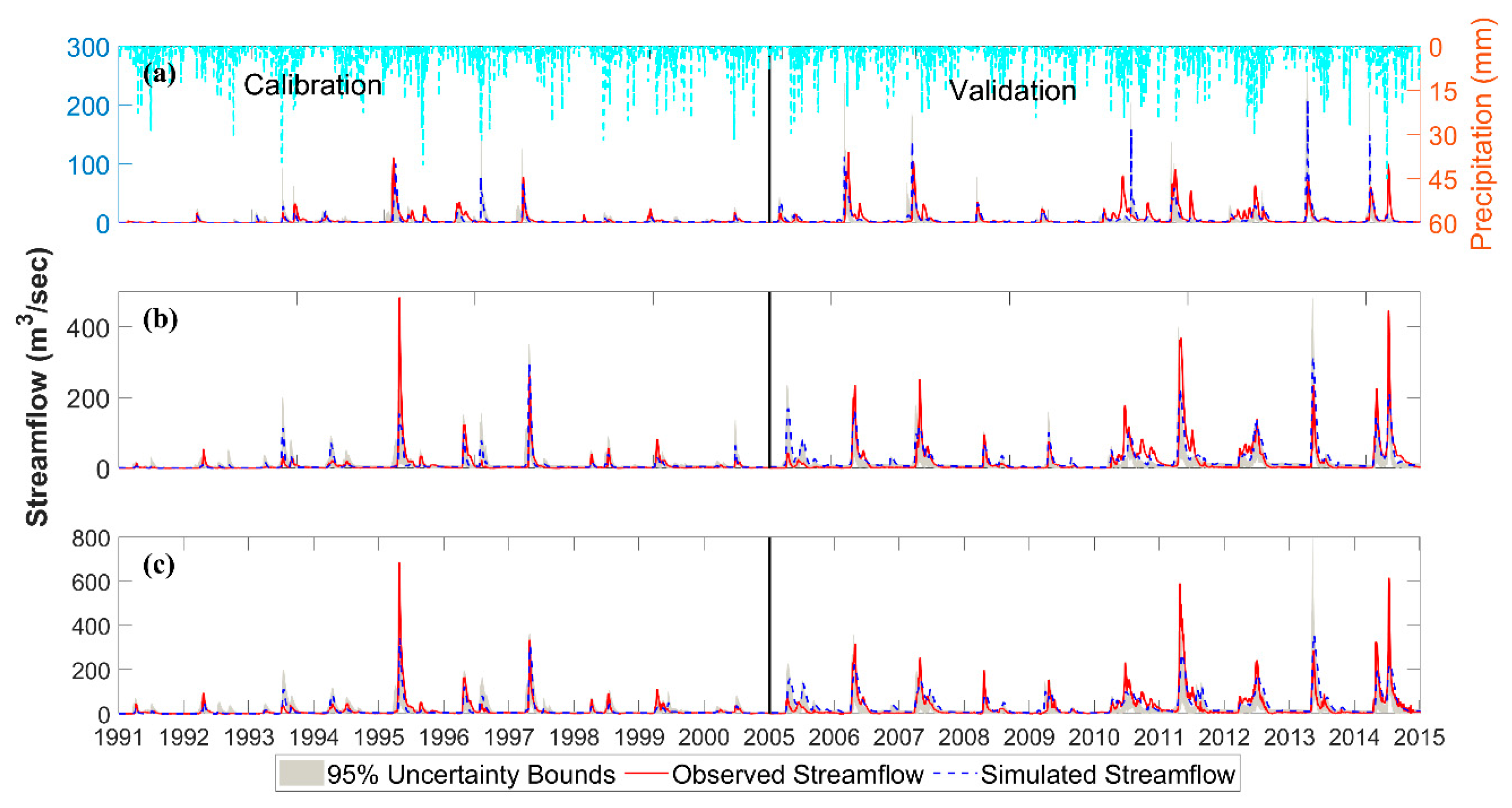
The initial range and fitted parameter values from model calibration are presented in Table 3. A procedure suggested by [49] was followed to better optimize parameters that govern hydrologic processes. For example, over prediction response of the model is controlled by decreasing CN2, increasing SOL_AWC, and ESCO. Similarly, low-flow (baseflow) response is corrected by increasing REVAPMN, and decreasing GWQMN, as well as decreasing GW_REVAP. The simulated and observed daily hydrographs for the upstream catchment (WSC station ID: 05MC001), mid catchment (WSC station ID: 05MD004) and reservoir inflow gauge (HFC station ID: 05MB999) are presented in Figure 4.
The model was able to produce simulated hydrographs that are representative of the observed daily average flow during the calibration and validation periods for all the three locations (Figure 4). Further, the model captured the trend in observed streamflow including the timing and duration of the peaks. The model, however, tended to under predict the larger peak flows (e.g., 1995, 2011, and 2014 events). The 1995 peak streamflow was estimated as a one in 100-year event, the 2011 as one in 300-year event, and the 2014 alike in size to that of 2011. To our understanding recreating such a large magnitude, low frequency events are almost impossible to predict. This is mainly because these events are rare in nature thus the data corresponding to such events are limited. Consequently, the model cannot be calibrated against these rare events due to insufficient data.
We further assessed model performance using multiple statistical metrics (Table 4). The rating of the model performance was based on the guideline presented by [47,49,53,54]. The performance of the model can be linked to the fitted parameters as all parameters are within suggested range [55] and reflect watershed hydrological processes. For example, the groundwater delay (GW_DELAY) parameter has a value of 479, which is close to the upper bound value. The GW_DELAY parameter represents the time taken by a water particle exiting the soil profile and entering the shallow aquifer. As our watershed is mostly clay, rich in organic matter, it makes sense to why the water particle takes such a long time in exiting the soil profile. Likewise, hydraulic conductivity through the bottom of the wetland (WET_K) is set at 0.33 mm h−1 which is within the range as set forth for this type of soils (https://structx.com/Soil_Properties_007.html).
3.3. Future Climate Projections Relative to Baseline Period
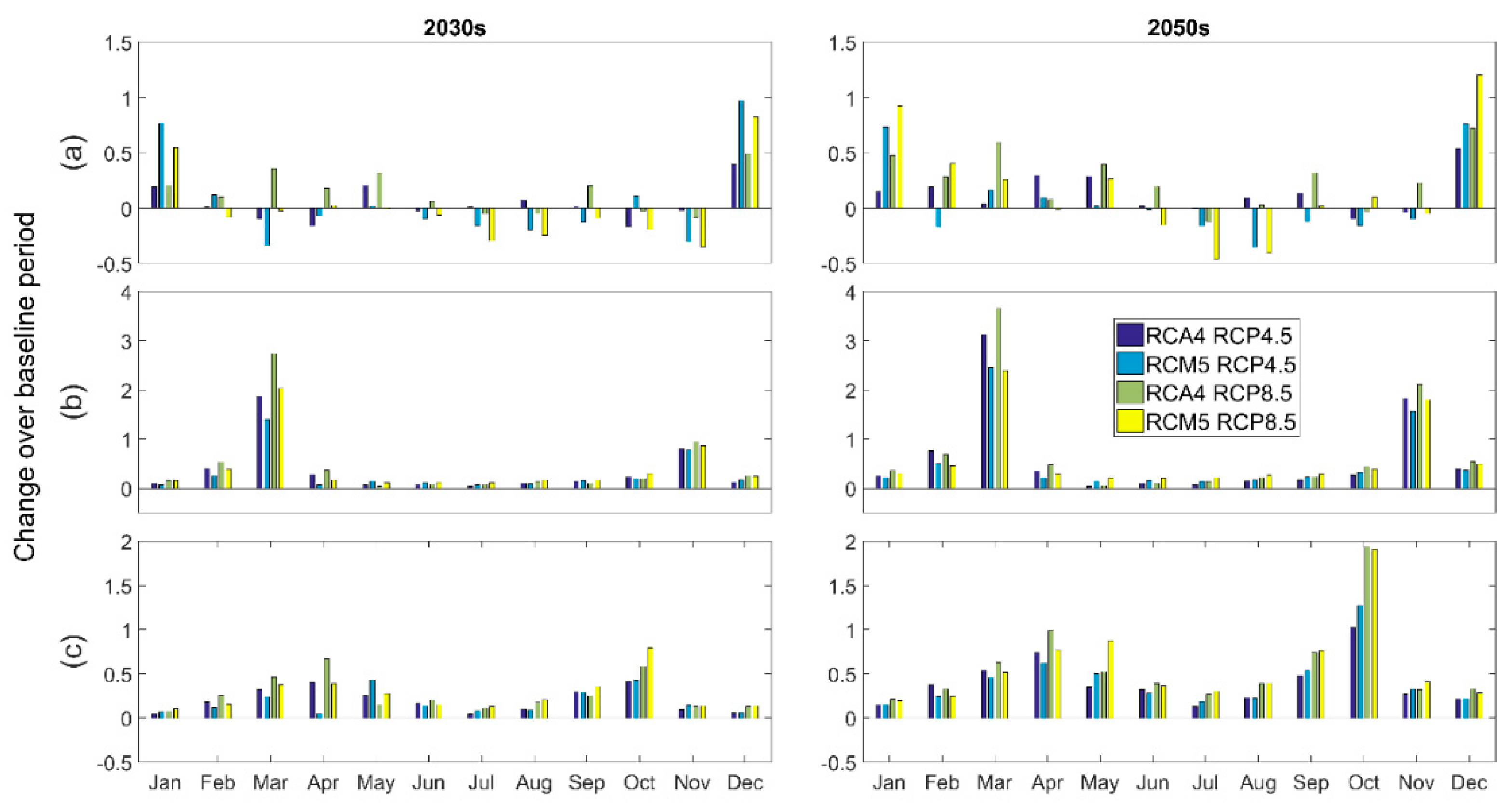
We first analyzed changes in future climate projections relative to baseline climate scenario (Figure 5). For ease of comparison, seasonally averaged values were used. The seasons are defined as winter: December, January, and February (DJF), spring: March, April, and May (MAM), summer: June, July, and August (JJA), and fall: September, October, and November (SON).
From the Figure 5a, precipitation increased during the winter under all scenarios and generally decreased during the summer. There is more consensus among scenarios from the two RCMs for temperature, projecting an increase in both maximum (Figure 5b) and minimum (Figure 5c) temperature over the catchment. The rise in temperature for the middle future (2050s) was markedly higher than the rise for the near future (2030s). On an annual average basis (Table 5), there was a 30% increase in temperature for the near future while there was a 52% increase for the middle future under both RCP 4.5 and 8.5, suggesting it is likely that the climate would continue to get warmer as we step further into the future. Regarding precipitation, RCA4 projected a 3.5% increase under RCP4.5, while RCM5 projected a 2% decrease for the near future. Under RCP8.5, RCA4 projected an 11% increase in precipitation compared to a 6% decrease in precipitation from RCM5 relative to the baseline period. For the middle future under RCP 4.5, RCA projected an 11% increase in precipitation while RCM5 projected a 2% decrease in precipitation. For RCP8.5, RCA4 projected a 20% increase in precipitation as compared to a 1% increase from RCM5.
Overall, there is agreement among the scenarios that conditions in the future for the basin are expected to be warmer and wetter in the winter months, with only one scenario (RCM5-RCP4.5) suggesting drier conditions in February. There was less agreement among scenarios in the spring and fall seasons, particularly for the near future (2030s), however, the scenarios more consistently projected drier summers and wetter winters. Combined with warmer temperatures across the basin, this is anticipated to increase winter flows and promote more drought-like summer conditions, which is in agreement with other climate change studies for the Prairies [16,25].
3.4. Impact of Future Climate Change on Streamflow
3.4.1. Overall Flow Regime
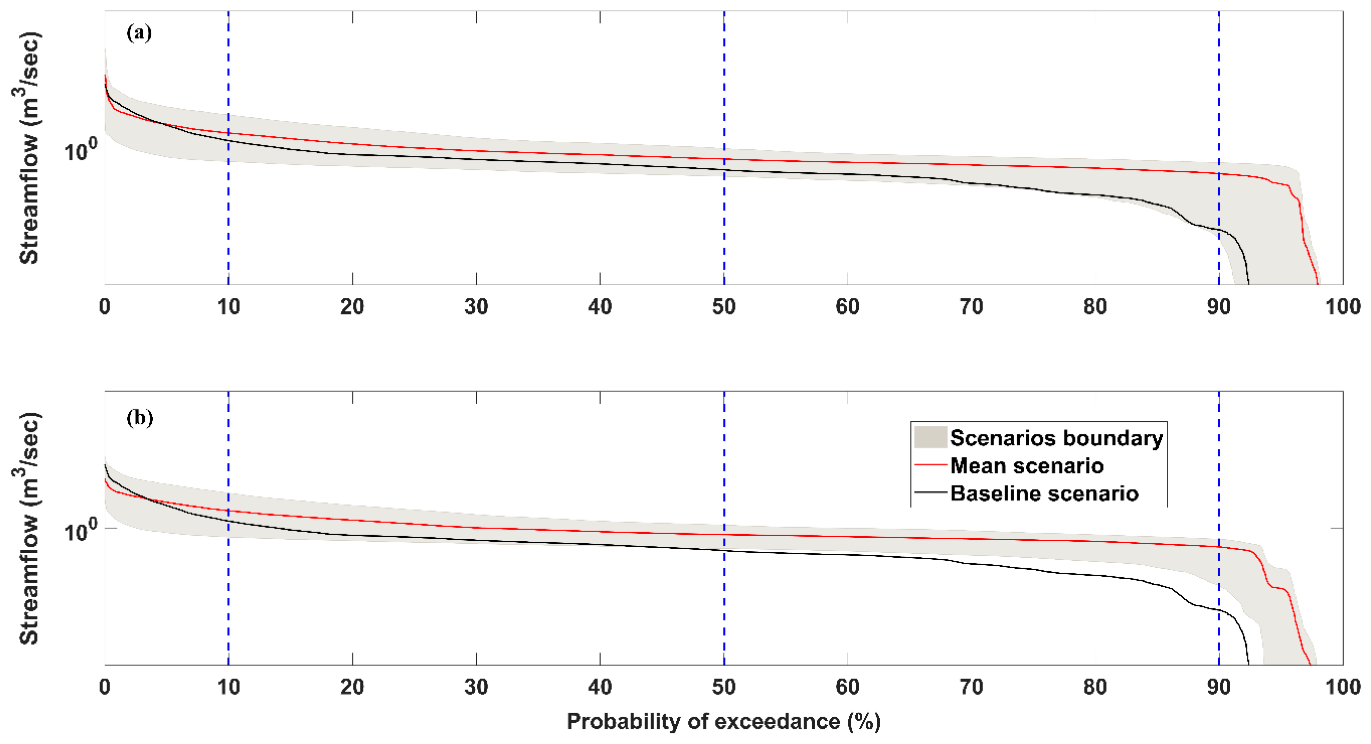
We assessed the overall flow regime of the future scenarios in comparison to baseline period using flow duration curves. The flow duration curve is a useful plot that shows the probability that flow will equal or exceed a specified value of interest. Figure 6 shows flow duration curve at reservoir inflow gauging point (HFC station ID: 05MB999) for baseline conditions: extreme climate (high and low), and the ensemble mean of the future climate scenarios, along with 10%, 50%, and 90% exceedance probabilities, using log10- normal probability curves to enhance the visibility of extreme quantiles.
In comparison to the baseline period (Figure 6), it can be observed that the probability of low and median flows has increased while the probability of high flows decreased under all future projections. These results suggest that, in the future, there will be more frequent occurrence of low flows, and less frequent occurrence of high flows. This is in agreement with the climate scenario results suggesting higher winter (low) flows due to warmer and wetter conditions and decreasing summer flows due to warmer and drier conditions [3]. Increasing low and median flows and decreasing peak flows result in a more uniform distribution of streamflow throughout the year, essentially ‘flattening’ the hydrograph (Figure 6). The lack of seasonal variability in streamflow is often not beneficial for the ecological community, and decreasing summer flows can result in higher stream temperatures which endanger fish populations [56]. Moderate fluctuations in streamflow stabilize channel structure through sediment transport and interaction between river and its floodplain and drives nutrient exchange and breeding cycles.
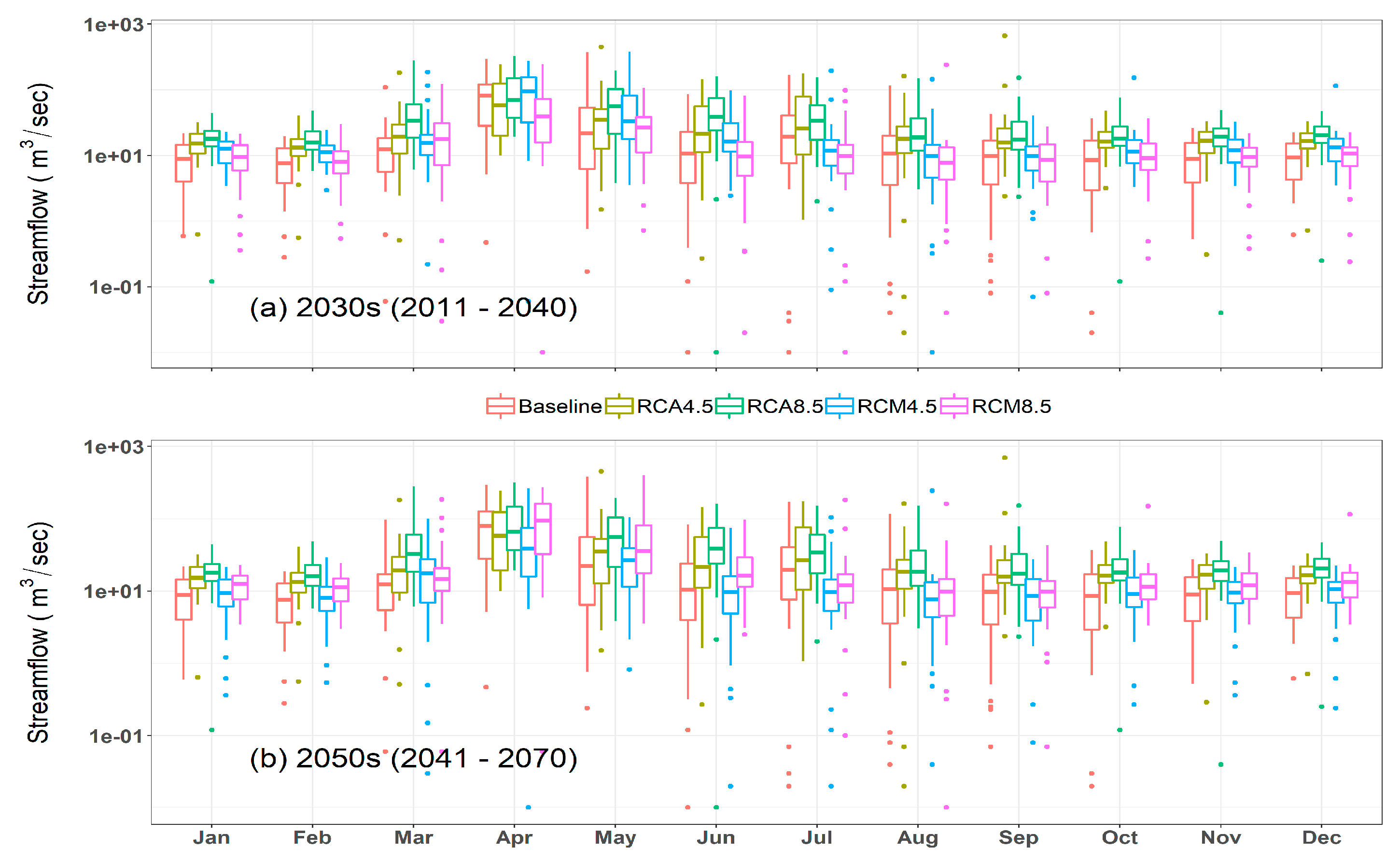
3.4.2. Mean Monthly Streamflow
All scenarios showed increasing streamflow during December, January, and March for both time periods i.e., 2030s and 2050s (Figure 7). Changes under RCA projections were, however, more aggressive in comparison to those resulting from the RCM, mostly predicting high flows, a feature that has previously been observed [57]. On an annual average basis, RCA scenarios showed increasing streamflow from 86% (RCP4.5) to 133% (RCP8.5) compared to 24% (RCP4.5) to 26% (RCP8.5) from the RCM scenarios over the 2011–2070 time period. During June to September, the RCM showed decreasing streamflow for both RCP scenarios and both time periods, consistent with warmer and drier conditions and the results previously reported by [3]. Increasing streamflow in the case of RCA could be linked to higher precipitation relative to the RCM scenarios for both near (2030s) and middle (2050s) under RCP4.5 and RCP8.5.
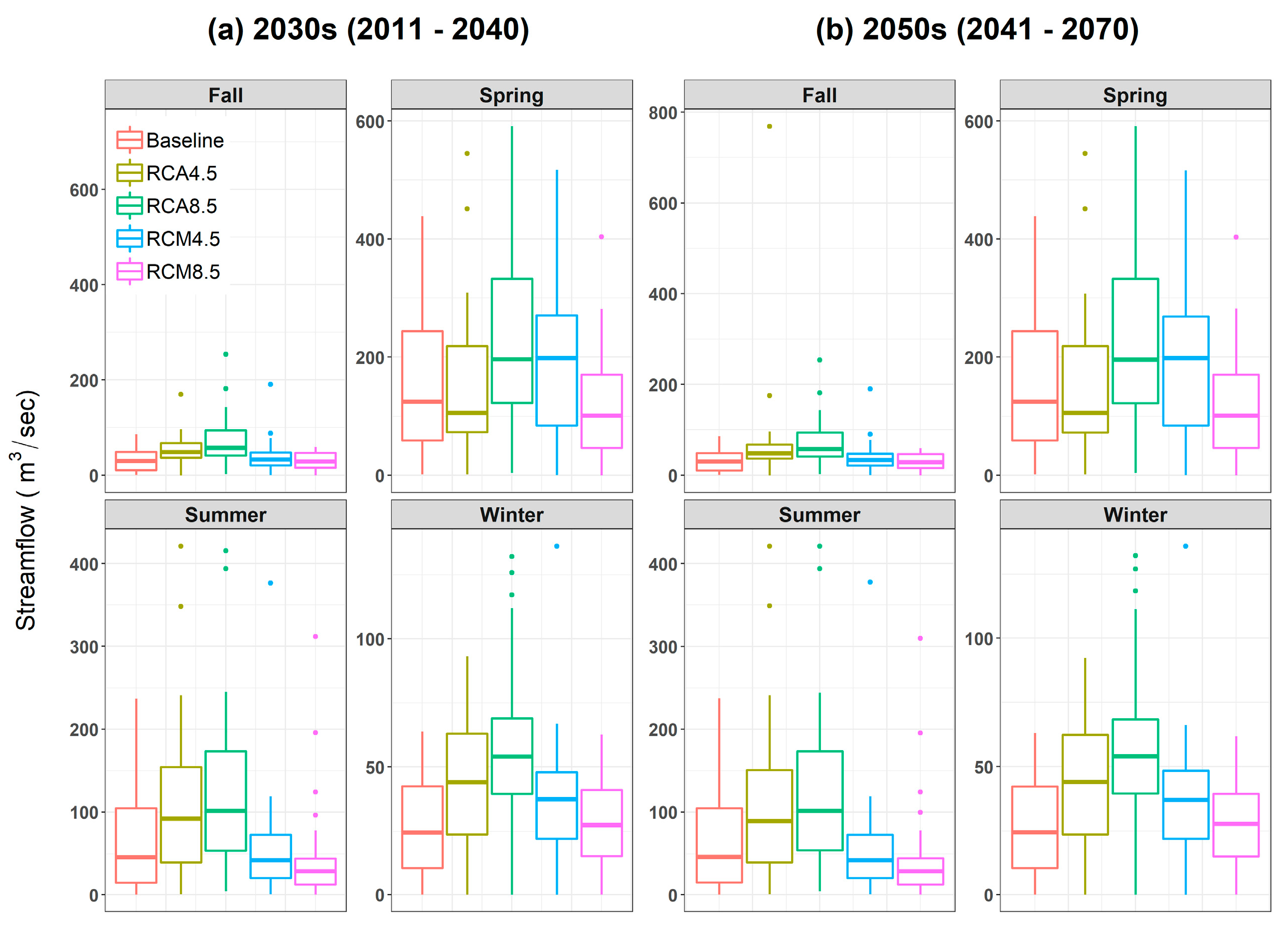
3.4.3. Seasonal Streamflow
We assessed the impact of climate change on seasonal flow for all climate projections, along with the baseline simulation (Figure 8). All climate change scenarios suggested a likely increase in winter flow (Figure 8a,b) due to the projected warmer and wetter conditions, with a likely increase in winter precipitation falling as rain and rain-on-snow events. The magnitude of change differs among RCPs and by model. RCA under RCP4.5 and RCP8.5 showed a likely increase of 66% to 110% during 2030s, whereas the RCM scenarios showed a 4%–40% increase in winter streamflow for the same time period. In the middle future (2050s), RCA showed 113% (RCP4.5) and 200% (RCP8.5) increased in winter flow compared to 48% (RCP4.5) and 120% (RCP8.5) from the RCM scenarios. The scenarios were in agreement, however, that winter flows will likely increase.
Both models however, projected opposing results for summer streamflow, with striking differences. RCA scenarios showed a likely increase of 76% under RCP4.5, up to a 155% increase under RCP8.5 for the 2030s; whereas RCM scenarios showed a decrease of 3% (RCP4.5)–23% (RCP8.5) for the same period. It is likely that disagreements in magnitude and direction of changing flow were the result of uncertainty in evapotranspiration response under higher temperatures (of differing magnitudes, depending on the scenario) and slightly higher moisture availability. Higher variability and uncertainty in summer flow regimes would have a significant impact on the future operation of the Shellmouth reservoir. For example, increasing winter flows would mean more water needs to be released throughout the winter. On the other hand, decreasing spring peaks and the potential for drier summers would require flows to be held back to address potential water supply shortages when demands are higher. Thus, predictability in seasonal variability is important for operations to mitigate any potential threat due flood and/or drought.
4. Discussions
This study had some limitations. Firstly, there were only three active meteorological stations available within the catchment, which were 100 km apart proximity. While calibration and validation of the model indicated satisfactory performance, our model may be further improved via use of gauges that are outside the catchment. Secondly, the study was only based on assessing the impact of climate change on the upstream water resources under stationary watershed conditions, ignoring the impact of land use and land cover changes. While climate change may likely be the main driver of changing hydrological regime of the watershed [3], incorporating land use change may further improve or complicate decision-making for reservoir control and management. Thirdly, the SWAT model works based on a weather generator that uses precipitation, temperature, wind speed, solar radiation, and relative humidity. Except precipitation and temperature, all other variables were taken from the NARR data set. Although the NARR dataset has been previously tested, showing good results across the study region [9], our model may be further improved by including ground-based observation stations to increase confidence in the modeling results. Fourthly, to expedite and manage simulation run time, a storage threshold was introduced to lump pothole wetlands, which affects the spatial representation these wetlands. Though the current concept is far better than the lumped representation of pothole wetlands [28,47], availability of a high performance computer could afford the full spatial representation of pothole wetlands to be implemented in the hydrologic model. Finally, due to resource limitation, climate projections from only two regional climate models were used, though these are the most up-to-date models, our analysis may be further improved via inclusion of more RCMs to add confidence on the overall climate change impact results.
The prairie pothole region is a hydrologically complex landscape with millions of pothole wetlands, left behind by the glacier activity about 10,000 years ago. The presence of these wetlands imposes significant challenges with respect to the use of hydrologic models in this region [58,59]. To date, there has not been an integrated approach taken to improve our understanding of how the region functions hydrologically [60]. Earlier studies proposed methods to capture the dynamics of variable contributing areas that incurred significant computational costs [32,34].
Our study represents an advance beyond preceding studies by implementing a threshold storage capacity to decrease computational costs and thereby facilitate climate change analyses.
Climate change projections rely on assumptions regarding future technological advances, economic and population growth, and natural processes such as changes in solar activity. Thus, there are numerous uncertainties in the climate models used to produce future climate change projections. These uncertainties may increase as they incorporate additional components of earth’s climate system—e.g., from projecting atmospheric circulation to projecting land surface interactions including soil and vegetation, also known as earth system modeling (ESM) [61]. Thus, assuming that the most up-to-date model will always perform better may not be true as investigated by several scholar [62,63]. While dynamic downscaling and bias corrected climate data may reduce uncertainty in individual model projections, each climate model is based on a unique set of mathematical equations that may provide unique climate projections. This is why we see differences in future streamflow projections while using forcing of the two difference climate models.
5. Conclusions
The Environment and Climate Change Canada (ECCC), in its latest report, indicated a projected 2.3–6.5 °C rise in surface temperature for the Canadian Prairies. Consequently, it is very likely that extreme precipitation events will become more intense and frequent, altering the hydrologic cycle and water availability of the region. Thus, the focus of the paper was on the use of modified SWAT model for assessing the impact of climate change on inflows to the Shellmouth reservoir across a prairie pothole region. The modified model was calibrated and validated using historical hydro-meteorological data, showing reasonably good simulation accuracy in both cases. A spatial calibration approach was adopted using all the available streamflow gauges in the catchment, making sure that the hydrology of each discretized piece of the watershed is reasonably replicated.
The study highlighted the important role that future climate projections would play in changing the hydrologic regime of the upper Assiniboine River Basin (UARB) catchment, especially its effect on the operation of the Shellmouth reservoir. All the climate change scenarios indicated a likely increase in winter streamflow. The increase in winter streamflow may require change of the operation rules of the reservoir in order to adapt the new changing reality. While RCA projected a likely increase in summer streamflow, the RCM suggest a 23% decrease. Water availability in summer season are of critical importance for the Shellmouth reservoir especially for meeting agricultural and water supply demands, thus serious adaptation strategies may need to be developed to address any potential water scarcity issues.
Although the model was specifically developed to assess climate change impact on the reservoir inflow, we see many other applications of the current concept. For example, the modified model can be expanded to the entire Assiniboine River Basin to evaluate couple impact of climate and land use change. Quantifying the coupled impact of climate and land use change on nutrient loading and how best management practices may reduce the overall nutrient export to the Lake Winnipeg are additional opportunities to apply our modified model.
Author Contributions
A.M. conceptualized, designed, analyzed results, and wrote original draft of the manuscript. G.R.E. helped with model source code modification. F.U. provided access to the HFC data bank, space, and computer resources. T.A.S. contributed to the design of the climate change study methodology, provided edits, and interpretation of the model results. All the co-authors review the manuscript prior to and during the submission process to the Water-MDPI Journal. All authors have read and agreed to the published version of the manuscript.
Funding
The Natural Sciences and Engineering Research Council (NSERC) of Canada provided funding, in part, to support this research through NSERC FloodNet (Grant number: NETGP 451456), a strategic research network. The Hydrologic Forecasting Centre (HFC) of Manitoba Infrastructure (MI) provided grants through Summer Temporary Employment Program (STEP).
Acknowledgments
The authors greatly appreciate the support, data, and other research related resources furnished by the Manitoba Hydrologic Forecast Centre of Manitoba Infrastructure (HFC-MI).
Conflicts of Interest
The authors declare no conflict of interest.
Disclaimer
This research article is the product of professional research and represents opinion of the authors. It is not meant to represent the opinion or position of the authors affiliated organization.
References
- Carvalho-Santos, C.; Monteiro, A.T.; Azevedo, J.C.; Honrado, J.P.; Nunes, J.P. Climate Change Impacts on Water Resources and Reservoir Management: Uncertainty and Adaptation for a Mountain Catchment in Northeast Portugal. Water Resour. Manag. 2017, 31, 3355–3370. [Google Scholar] [CrossRef] [Green Version]
- Park, J.Y.; Park, M.J.; Ahn, S.R.; Park, G.A.; Yi, J.E.; Kim, G.S.; Srinivasan, R.; Kim, S.J. Assessment of future climate change impacts on water quantity and quality for a mountainous dam watershed using SWAT. Am. Soc. Agric. Biol. Eng. 2011, 54, 1725–1737. [Google Scholar]
- Muhammad, A.; Evenson, G.R.; Stadnyk, T.A.; Boluwade, A.; Jha, S.K.; Coulibaly, P. Assessing the importance of potholes in the Canadian Prairie Region under future climate change scenarios. Water 2018, 10, 1657. [Google Scholar] [CrossRef] [Green Version]
- Dibike, Y.; Prowse, T.; Bonsal, B.; O’Neil, H. Implications of future climate on water availability in the western Canadian river basins. Int. J. Climatol. 2017, 37, 3247–3263. [Google Scholar] [CrossRef]
- Zheng, H.; Chiew, F.H.S.; Charles, S.; Podger, G. Future climate and runoff projections across South Asia from CMIP5 global climate models and hydrological modelling. J. Hydrol. Reg. Stud. 2018, 18, 92–109. [Google Scholar] [CrossRef]
- Wang, K.; Dickinson, R.E.; Liang, S.; Wang, K.; Dickinson, R.E.; Liang, S. Global Atmospheric Evaporative Demand over Land from 1973 to 2008. J. Clim. 2012, 25, 8353–8361. [Google Scholar] [CrossRef]
- Barnett, T.P.; Adam, J.C.; Lettenmaier, D.P. Potential impacts of a warming climate on water availability in snow-dominated regions. Nature 2005, 438, 303–309. [Google Scholar] [CrossRef] [PubMed]
- Kumar, N.; Tischbein, B.; Kusche, J.; Laux, P.; Beg, M.K.; Bogardi, J.J. Impact of climate change on water resources of upper Kharun catchment in Chhattisgarh, India. J. Hydrol. Reg. Stud. 2017, 13, 189–207. [Google Scholar] [CrossRef]
- Shrestha, R.R.; Dibike, Y.B.; Prowse, T.D. Modelling of climate-induced hydrologic changes in the Lake Winnipeg watershed. J. Gt. Lakes Res. 2012, 38, 83–94. [Google Scholar] [CrossRef]
- Johnson, W.C.; Poiani, K.A. Climate Change Effects on Prairie Pothole Wetlands: Findings from a Twenty-five Year Numerical Modeling Project. Wetlands 2016, 36, 273–285. [Google Scholar] [CrossRef]
- Qian, B.; De Jong, R.; Huffman, T.; Wang, H.; Yang, J. Projecting yield changes of spring wheat under future climate scenarios on the Canadian Prairies. Theor. Appl. Climatol. 2016, 123, 651–669. [Google Scholar] [CrossRef]
- Betts, A.K.; Desjardins, R.; Worth, D.; Cerkowniak, D. Impact of land use change on the diurnal cycle climate of the Canadian Prairies. J. Geophys. Res. Atmos. 2013, 118, 11-996. [Google Scholar] [CrossRef]
- Herring, S.C.; Hoerling, M.P.; Kossin, J.P.; Peterson, T.C.; Stott, P.A.; Herring, S.C.; Hoerling, M.P.; Kossin, J.P.; Peterson, T.C.; Stott, P.A. Explaining Extreme Events of 2014 from a Climate Perspective. Bull. Am. Meteorol. Soc. 2015, 96. [Google Scholar] [CrossRef]
- Brath, B.; Friesen, T.; Guérard, Y.; Jacques-Brissette, C.; Lindman, C.; Lockridge, K.; Mulgund, S.; Walke, B.-J. Climate Change and Resource Sustainability: An Overview for Actuaries; Canadian Institute of Actuaries: Ottawa, ON, Canada, 2015; pp. 1–57. [Google Scholar]
- Olmstead, S.M. Climate change adaptation and water resource management: A review of the literature. Energy Econ. 2014, 46, 500–509. [Google Scholar] [CrossRef]
- Bush, E.; Lemmen, D.S. Canada’s Changing Climate Report; Environment and Climate Change Canada, Government of Canada: Ottawa, ON, Canada, 2019; ISBN 978-0-660-30222-5. [Google Scholar]
- Shrestha, R.R.; Dibike, Y.B.; Prowse, T.D. Modeling Climate Change Impacts on Hydrology and Nutrient Loading in the Upper Assiniboine Catchmen. J. Am. Water Resour. Assoc. 2012, 48, 74–89. [Google Scholar] [CrossRef]
- Zhang, H.; Huang, G.H.; Wang, D.; Zhang, X. Uncertainty assessment of climate change impacts on the hydrology of small prairie wetlands. J. Hydrol. 2011, 396, 94–103. [Google Scholar] [CrossRef] [Green Version]
- Zhang, H.; Huang, G.H. Development of climate change projections for small watersheds using multi-model ensemble simulation and stochastic weather generation. Clim. Dyn. 2013, 40, 805–821. [Google Scholar] [CrossRef]
- Dumanski, S.; Pomeroy, J.W.; Westbrook, C.J. Hydrological regime changes in a Canadian Prairie basin. Hydrol. Process. 2015, 29, 3893–3904. [Google Scholar] [CrossRef]
- Clark, R.; Andreichuk, I.; Sauchyn, D.; McMartin, D.W. Incorporating climate change scenarios and water-balance approach to cumulative assessment models of solution potash Mining in the Canadian Prairies. Clim. Chang. 2017, 145, 321–334. [Google Scholar] [CrossRef]
- Joyce, C.B.; Simpson, M.; Casanova, M. Future wet grasslands: Ecological implications of climate change. Ecosyst. Health Sustain. 2016, 2, e01240. [Google Scholar] [CrossRef] [Green Version]
- Gaur, A.; Gaur, A.; Simonovic, S.P. Future Changes in Flood Hazards across Canada under a Changing Climate. Water 2018, 10, 1441. [Google Scholar] [CrossRef] [Green Version]
- O’Neil, H.C.L.; Prowse, T.D.; Bonsal, B.R.; Dibike, Y.B. Spatial and temporal characteristics in streamflow-related hydroclimatic variables over western Canada. Part 1: 1950–2010. Hydrol. Res. 2017, 48, 915–931. [Google Scholar] [CrossRef]
- St-Jacques, J.-M.; Andreichuk, Y.; Sauchyn, D.J.; Barrow, E. Projecting Canadian Prairie Runoff for 2041–2070 with North American Regional Climate Change Assessment Program (NARCCAP) Data. JAWRA J. Am. Water Resour. Assoc. 2018, 54, 660–675. [Google Scholar] [CrossRef]
- Spence, C.; Woo, M. Hydrology of subarctic Canadian shield: Soil-filled valleys. J. Hydrol. 2003, 279, 151–166. [Google Scholar] [CrossRef]
- Shook, K.; Pomeroy, J.W.; Spence, C.; Boychuk, L. Storage dynamics simulations in prairie wetland hydrology models: Evaluation and parameterization. Hydrol. Process. 2013, 27, 1875–1889. [Google Scholar] [CrossRef]
- Evenson, G.R.; Golden, H.E.; Lane, C.R.; Amico, E.D.; D’Amico, E. Geographically isolated wetlands and watershed hydrology: A modified model analysis. J. Hydrol. 2015, 529, 240–256. [Google Scholar] [CrossRef] [Green Version]
- Zhang, Z.; Stadnyk, T.A.; Burn, D.H. Identification of a preferred statistical distribution for at-site flood frequency analysis in Canada. Can. Water Resour. J. Rev. Can. Ressour. Hydr. 2019. [Google Scholar] [CrossRef]
- Shook, K. Complexity of Prairie Hydrology Distinctiveness of Prairie Hydrology. Available online: https://www.google.com.sg/url?sa=t&rct=j&q=&esrc=s&source=web&cd=1&ved=2ahUKEwjN3uz53onnAhXaad4KHVTGBpAQFjAAegQIBhAB&url=https%3A%2F%2Fwiki.usask.ca%2Fdownload%2Fattachments%2F516948256%2F01_ComplexityOfPrairieHydrology_KShook.pdf&usg=AOvVaw1gWgzZDRY-iJiVc6aiSERo (accessed on 16 January 2020).
- Mekonnen, B.A.; Mazurek, K.A.; Putz, G. Incorporating landscape depression heterogeneity into the Soil and Water Assessment Tool (SWAT) using a probability distribution. Hydrol. Process. 2016, 30, 2373–2389. [Google Scholar] [CrossRef]
- Evenson, G.R.; Golden, H.E.; Lane, C.R.; D’Amico, E. An improved representation of geographically isolated wetlands in a watershed-scale hydrologic model. Hydrol. Process. 2016, 30, 4168–4184. [Google Scholar] [CrossRef]
- Wang, X.; Yang, W.; Melesse, A.M. Using hydrologic equivalent wetland concept within SWAT to estimate streamflow in watersheds with numerous wetlands. Trans. ASABE 2008, 51, 55–72. [Google Scholar] [CrossRef]
- Muhammad, A.; Evenson, G.R.; Stadnyk, T.A.; Boluwade, A.; Jha, S.K.; Coulibaly, P. Impact of model structure on the accuracy of hydrological modeling of a Canadian Prairie watershed. J. Hydrol. Reg. Stud. 2019, 21, 40–56. [Google Scholar] [CrossRef]
- Olthof, I.; Latifovic, R.; Pouliot, D. Development of a circa 2000 land cover map of northern Canada at 30 m resolution from Landsat. Can. J. Remote Sens. 2009, 35, 152–165. [Google Scholar] [CrossRef]
- Saskatchewan Water Security Agency. Upper Assiniboine River Basin Study; Saskatchewan Water Security Agency: Moose Jaw, SK, Canada, 2000. [Google Scholar]
- Neitsch, S.L.; Arnold, J.G.; Kiniry, J.R.; Williams, J.R. Soil and Water Assessment Tool Theoretical Documentation Version 2009; Texas Water Resources Institute: Forney, TX, USA, 2011; Available online: http://hdl.handle.net/1969.1/128050 (accessed on 16 January 2020).
- Gassman, P.W.; Reyes, M.R.; Green, C.H.; Arnold, J.G.; Gassman, P.W. The soil and water assessment tool: Historical development, applications, and future research directions. Trans. ASABE 2007, 50, 1211–1250. [Google Scholar] [CrossRef] [Green Version]
- Muhammad, A.; Stadnyk, T.A.; Unduche, F.; Coulibaly, P. Multi-Model Approaches for Improving Seasonal Ensemble Streamflow Prediction Scheme with Various Statistical Post-Processing Techniques in the Canadian Prairie Region. Water 2018, 10, 1604. [Google Scholar] [CrossRef] [Green Version]
- Soil Landscapes of Canada Working Group Soil Landscapes of Canada Version 3.2. Available online: http://sis.agr.gc.ca/cansis/nsdb/slc/v3.2/index.html (accessed on 5 December 2018).
- NRC. Level 1 Canadian Digital Elevation Data Product Specifications; NRC: Ottawa, ON, Canada, 2007. [Google Scholar]
- Mesinger, F.; DiMego, G.; Kalnay, E.; Mitchell, K.; Shafran, P.C.; Ebisuzaki, W.; Jović, D.; Woollen, J.; Rogers, E.; Berbery, E.H.; et al. North American Regional Reanalysis. Bull. Am. Meteorol. Soc. 2006, 87, 343–360. [Google Scholar] [CrossRef] [Green Version]
- Mearns, L.O.; McGinnis, S.; Korytina, D.; Arritt, R.; Biner, S.; Bukovsky, M. The NA-CORDEX Dataset, Version 1.0; NCAR Climate Data Gateway: Boulder, CO, USA, 2017. [Google Scholar]
- Abbaspour, K.C.; Yang, J.; Maximov, I.; Siber, R.; Bogner, K.; Mieleitner, J.; Zobrist, J.; Srinivasan, R. Modelling hydrology and water quality in the pre-alpine/alpine Thur watershed using SWAT. J. Hydrol. 2007, 333, 413–430. [Google Scholar] [CrossRef]
- Abbaspour, K.C.; Johnson, C.A.; van Genuchten, M.T. Estimating Uncertain Flow and Transport Parameters Using a Sequential Uncertainty Fitting Procedure. Vadose Zone J. 2004, 3, 1340–1352. [Google Scholar] [CrossRef]
- Zhang, X.; Srinivasan, R.; Van Liew, M.; Van Liew, M.; Member, A. Multi-Site Calibration of the Swat Model for Hydrologic Modeling. Trans ASABE 2008, 51, 2039–2049. [Google Scholar] [CrossRef] [Green Version]
- Gupta, H.V.; Kling, H.; Yilmaz, K.K.; Martinez, G.F. Decomposition of the mean squared error and NSE performance criteria: Implications for improving hydrological modelling. J. Hydrol. 2009, 377, 80–91. [Google Scholar] [CrossRef] [Green Version]
- Pechlivanidis, I.G.; Arheimer, B. Large-scale hydrological modelling by using modified PUB recommendations: The India-HYPE case. Hydrol. Earth Syst. Sci. 2015, 19, 4559–4579. [Google Scholar] [CrossRef] [Green Version]
- Abbaspour, K.C.; Rouholahnejad, E.; Vaghefi, S.; Srinivasan, R.; Yang, H.; Kløve, B. A continental-scale hydrology and water quality model for Europe: Calibration and uncertainty of a high-resolution large-scale SWAT model. J. Hydrol. 2015, 524, 733–752. [Google Scholar] [CrossRef] [Green Version]
- Riahi, K.; Rao, S.; Krey, V.; Cho, C.; Chirkov, V.; Fischer, G.; Kindermann, G.; Nakicenovic, N.; Rafaj, P. RCP 8.5—A scenario of comparatively high greenhouse gas emissions. Clim. Chang. 2011, 109, 33–57. [Google Scholar] [CrossRef] [Green Version]
- Collins, M.; Knutti, R.; Arblaster, J.; Dufresne, J.-L.; Fichefet, T.; Friedlingstein, P.; Gao, X.; Gutowski, W.J.; Johns, T.; Krinner, G.; et al. Chapter 12—Long-term climate change: Projections, commitments and irreversibility. In Climate Change 2013: The Physical Science Basis; IPCC Working Group I Contribution to AR5; IPCC, Ed.; Cambridge University Press: Cambridge, UK, 2013. [Google Scholar]
- Vieira, M.J.F. 738 Years of Global Climate Model Simulated Streamflow in the Nelson-Churchill River Basin. Master’s Thesis, University of Manitoba, Winnipeg, MB, Canada, 2016. [Google Scholar]
- Moriasi, D.N.; Arnold, J.G.; Van Liew, M.W.; Binger, R.L.; Harmel, R.D.; Veith, T.L. Model evaluation guidelines for systematic quantification of accuracy in watershed simulations. Trans. ASABE 2007, 50, 885–900. [Google Scholar] [CrossRef]
- Singh, J.; Knapp, H.V.; Arnold, J.G.; Demissie, M. Hydrological modeling of the Iroquois River watershed using HSPF and SWAT. J. Am. Water Resour. Assoc. 2005, 41, 343–360. [Google Scholar] [CrossRef]
- Abbaspour, K.; Vejdani, M.; Haghighat, S. SWAT-CUP calibration and uncertainty programs for SWAT. In Proceedings of the MODSIM 2007 International Congress on Modelling and Simulation, Modelling and Simulation Society of Australia and New Zealand, Melbourne, Australia, 1–6 December 2007; pp. 1596–1602. [Google Scholar]
- Du, X.; Shrestha, N.K.; Wang, J. Assessing climate change impacts on stream temperature in the Athabasca River Basin using SWAT equilibrium temperature model and its potential impacts on stream ecosystem. Sci. Total Environ. 2019, 650, 1872–1881. [Google Scholar] [CrossRef] [PubMed]
- Dosio, A. Projections of climate change indices of temperature and precipitation from an ensemble of bias-adjusted high-resolution EURO-CORDEX regional climate models. J. Geophys. Res. Atmos. 2016, 121, 5488–5511. [Google Scholar] [CrossRef]
- Muhammad, A. Uncertainty in Streamflow Simulation of the Upper Assiniboine River Basin. PhD Thesis, University of Manitoba, Winnipeg, MB, Canada, 2019. [Google Scholar]
- Muhammad, A.; Jha, S.; Rasmussen, P. Challenges and Model Limitations in Predicting Streamflow in the Canadian Prairie Region; Flash FloodNet. 2016. Available online: https://uploads-ssl.webflow.com/5dc2ef924a9b7e7f028da6f7/5de676baec6ca43a0e1cff53_FlashFloodNet_Vol2.pdf (accessed on 16 January 2020).
- Spence, C.; Wolfe, J.D.; Whitfield, C.J.; Baulch, H.M.; Basu, N.B.; Bedard-Haughn, A.K.; Belcher, K.W.; Clark, R.G.; Ferguson, G.A.; Hayashi, M.; et al. Prairie water: A global water futures project to enhance the resilience of prairie communities through sustainable water management. Can. Water Resour. J. Rev. Can. Ressour. Hydr. 2019, 44, 115–126. [Google Scholar] [CrossRef]
- USGCRP. Climate Science Special Report. Available online: https://science2017.globalchange.gov/chapter/4/ (accessed on 30 December 2019).
- Kumar, D.; Kodra, E.; Ganguly, A.R. Regional and seasonal intercomparison of CMIP3 and CMIP5 climate model ensembles for temperature and precipitation. Clim. Dyn. 2014, 43, 2491–2518. [Google Scholar] [CrossRef]
- Knutti, R.; Sedláček, J. Robustness and uncertainties in the new CMIP5 climate model projections. Nat. Clim. Chang. 2013, 3, 369–373. [Google Scholar] [CrossRef]
Figure 1.
Geospatial location of the Upper Assiniboine River basin including the Shellmouth reservoir (Lake of the Prairie): (a) shows area of interest in Canada while (b) shows study area along with major cities and hydrometric stations utilized to construct the model.
Figure 1.
Geospatial location of the Upper Assiniboine River basin including the Shellmouth reservoir (Lake of the Prairie): (a) shows area of interest in Canada while (b) shows study area along with major cities and hydrometric stations utilized to construct the model.

Figure 2.
Hydro-climatic data of the Upper Assiniboine River basin at Shellmouth reservoir: mean monthly precipitation (mm), mean monthly streamflow (m3/s), and mean monthly average temperature (°C) over 1988–2017 time period.
Figure 2.
Hydro-climatic data of the Upper Assiniboine River basin at Shellmouth reservoir: mean monthly precipitation (mm), mean monthly streamflow (m3/s), and mean monthly average temperature (°C) over 1988–2017 time period.

Figure 3.
Decision tree of the modified SWAT wetland module based on the specified threshold concept.
Figure 3.
Decision tree of the modified SWAT wetland module based on the specified threshold concept.

Figure 4.
Calibration and validation result for the Upper Assiniboine River basin at (a) upstream catchment (WSC station ID: 05MC001) with precipitation on the secondary axis, (b) mid-stream catchment (WSC station ID: 05MD004), and (c) lower stream catchment or reservoir inflow gauging point (HFC station ID: 05MB999).

Figure 5.
Average annual monthly bias corrected projected change in climate variables relative to the baseline period (1988—2017): (a) precipitation in mm, (b) maximum temperature in °C, and (c) minimum temperature in °C.
Figure 5.
Average annual monthly bias corrected projected change in climate variables relative to the baseline period (1988—2017): (a) precipitation in mm, (b) maximum temperature in °C, and (c) minimum temperature in °C.

Figure 6.
Streamflow duration curve of the Upper Assiniboine River basin at Shellmouth reservoir (HFC station ID: 05MB999) for all climate change scenarios over the period (a) 2030s (2011–2040), and (b) 2050s (2041–2070).
Figure 6.
Streamflow duration curve of the Upper Assiniboine River basin at Shellmouth reservoir (HFC station ID: 05MB999) for all climate change scenarios over the period (a) 2030s (2011–2040), and (b) 2050s (2041–2070).

Figure 7.
Average projected mean monthly streamflow for the (a) 2030s and (b) 2050s under RCP4.5 and RCP8.5 along with the baseline simulation (1988–2017). Whiskers are 1.5 times the interquartile range.
Figure 7.
Average projected mean monthly streamflow for the (a) 2030s and (b) 2050s under RCP4.5 and RCP8.5 along with the baseline simulation (1988–2017). Whiskers are 1.5 times the interquartile range.

Figure 8.
Seasonal streamflow boxplot for (a) 2030s (2011–2040) and (b) 2050s (2041–2070) under RCP4.5 and RCP8.5 for all climate change scenarios at the reservoir inflow point (HFC-MI gauge: 05MB999) along with the baseline simulation (1988–2017).
Figure 8.
Seasonal streamflow boxplot for (a) 2030s (2011–2040) and (b) 2050s (2041–2070) under RCP4.5 and RCP8.5 for all climate change scenarios at the reservoir inflow point (HFC-MI gauge: 05MB999) along with the baseline simulation (1988–2017).


Table 1.
Input data sources and description used to configure the soil water assessment tool (SWAT) model.
Table 1.
Input data sources and description used to configure the soil water assessment tool (SWAT) model.
| Data Type | Application | Source | Reference |
|---|---|---|---|
| Land use | Land use properties | http://geogratis.gc.ca/ | [35] |
| Soil type | Soil properties | http://www.agr.gc.ca/ | [40] |
| Digital Elevation Model | Catchment delineation, channel slopes, and length | http://geogratis.gc.ca/ | [41] |
| Reservoir feature | Fully supply level, storage capacity, surface area, etc. | https://www.gov.mb.ca/ | HFC-MI 1 |
| Weather | Precipitation and temperature | https://weather.gc.ca/ | ECCC 2 |
| NARR data | Wind speed, relative humidity, and solar radiation | ftp://nomads.ncdc.noaa.gov/NARR/ | [42] |
| Climate change | Future climate change projections | https://na-cordex.org | [43] |
| Streamflow | Model calibration and validation | https://wateroffice.ec.gc.ca/ | WSC 3 |
1 Hydrologic Forecasting Centre of Manitoba Infrastructure; 2 Environment and Climate Change Canada; 3 Water Survey of Canada.
Table 2.
Hydro-meteorological stations utilized to construct Shellmouth reservoir SWAT model.
| S. No | Station ID | Operator | Station Name | Latitude | Longitude |
|---|---|---|---|---|---|
| Hydrometric Stations | |||||
| 1 | 05MC001 | WSC 1 | Assiniboine River at Sturgis | 51.94 | −102.54 |
| 2 | 05MB003 | WSC | Whitesand River near Canora | 51.63 | −102.36 |
| 3 | 05MD004 | WSC | Assiniboine River at Kamsack | 51.56 | −101.91 |
| 4 | 05MB001 | WSC | Yorkton creek near Ebenezer | 51.36 | −102.49 |
| 5 | 05MD005 | WSC | Shell River near Inglis | 50.96 | −101.31 |
| 6 | 05MD999 | HFC–MI 2 | Shellmouth reservoir inflow | 50.97 | −101.42 |
| Meteorological Stations | |||||
| 1 | 5040FJ3 | CCN 3 | Cowan | 52.03 | −100.65 |
| 2 | 4013660 | CCN | Kelliher | 51.26 | −103.75 |
| 3 | 4014145 | CCN | Langenburg | 50.90 | −101.72 |
| 4 | 4085052 | CCN | Mckague 2 | 52.58 | −103.83 |
| 5 | 4086000 | ECCC 4 | Pelly | 52.08 | −101.87 |
| 6 | 4086001 | ECCC | Pelly 2 | 51.73 | −101.90 |
| 7 | 5012469 | ECCC | Roblin | 51.18 | −101.37 |
| 8 | 501B4G2 | CCN | Roblin Friesen 3 Northwest | 51.27 | −101.40 |
| 9 | 4019082 | ECCC | Tonkin | 51.20 | −102.23 |
| 10 | 4019073 | ECCC | Yorkton | 51.26 | −102.46 |
| 11 | 501KE01 | CCN | Rossburn 4 North | 50.75 | −100.82 |
1 Water Survey of Canada; 2 Hydrologic Forecasting Centre of Manitoba Infrastructure; 3 Co-operative Climate Network; 4 Environment and Climate Change Canada.
Table 3.
Initial and final calibrated parameters for the Shellmouth reservoir catchment in the Upper Assiniboine River Basin (UARB).
Table 3.
Initial and final calibrated parameters for the Shellmouth reservoir catchment in the Upper Assiniboine River Basin (UARB).
| Parameter | Parameter Range | Descriptions (Units, If Applicable) | ||
|---|---|---|---|---|
| Min | Max | Fitted Value | ||
| ALPHA_BF | 0.01 | 0.80 | 0.36 | Base flow alpha factor (days) |
| GW_DELAY | 0.00 | 500.00 | 479.92 | Groundwater delays (days) |
| GW_REVAP | 0.02 | 0.20 | 0.11 | Groundwater revap coefficient |
| GWQMN | 0.00 | 5000.00 | 4978.00 | Threshold depth of water in the shallow aquifer required for return flow (mm) |
| RCHRG_DP | 0.00 | 1.00 | 0.15 | Deep aquifer percolation faction |
| REVAPMN | 0.00 | 500.00 | 296.93 | Threshold depth of water in the shallow aquifer required for revap to occur (mm) |
| CH_K1 | 0.00 | 150.00 | 21.26 | Effective hydraulic conductivity in tributary channel alluvium (mm h−1) |
| CH_K2 | 0.00 | 150.00 | 108.35 | Effective hydraulic conductivity in main channel alluvium (mm h−1) |
| CH_N1 | 0.01 | 0.30 | 0.17 | Manning’s N value for the tributary channel |
| CH_N2 | 0.01 | 0.30 | 0.10 | Manning’s N value for the main channel |
| CN2 a | −0.25 | 0.25 | −0.03 | SCS runoff curve number |
| SOL_AWC a | −0.25 | 0.25 | −0.18 | Available water capacity (mm H2O mm−1) |
| EPCO | 0.00 | 1.00 | 0.58 | Plant uptake compensation factor |
| ESCO | 0.00 | 1.00 | 0.41 | Soil evaporation compensation factor |
| TIMP | 0.01 | 1.00 | 0.18 | Snowpack temperature lag factor |
| SFTMP | −3.00 | 3.00 | 0.06 | Snowfall temperature |
| SMTMP | −3.00 | 3.00 | 0.41 | Snowmelt base temperature |
| SMFMN | 0.00 | 10.00 | 1.71 | Melt factor for snow on winter solstice (mm c−1 day−1) |
| SNOCOVMX | 5.00 | 500.00 | 174.86 | Minimum snow water content that corresponds to 100% snow cover (mm) |
| SNO50COV | 0.05 | 0.80 | 0.21 | Snow water equivalent that corresponds to 50% snow cover (%) |
| SMFMX | 0.00 | 10.00 | 8.18 | Maximum melt rate for snow on summer solstice (mm c−1 day−1) |
| OV_N a | −0.20 | 0.20 | 0.56 | Manning’s N value for overland flow |
| CH_L1 a | −1.00 | 1.00 | 0.44 | Longest tributary channel length in sub basin |
| CH_W1 a | −1.00 | 1.00 | 0.16 | Average width of tributary channels (m) |
| CH_L2 a | −1.00 | 1.00 | −0.31 | Length of main channel (m) |
| CH_W2 a | −1.00 | 1.00 | 0.21 | Average width of main channel (m) |
| WET_K | 0.00 | 3.60 | 0.33 | Hydraulic conductivity of bottom of wetland (mm h−1) |
a Parameters handled with relative change.
Table 4.
Statistical measure of baseline model performance: Calibration (1991–2000) validation (2005–2014).
Table 4.
Statistical measure of baseline model performance: Calibration (1991–2000) validation (2005–2014).
| Model Performance at Daily Time Step: Calibration (Validation) | ||||||
|---|---|---|---|---|---|---|
| Station Code | Station Name | p-Factor | r-Factor | KGE | R2 | PBIAS |
| 05MC001 | Assiniboine River at Sturgis | 0.7 (0.7) | 0.6 (0.5) | 0.7 (0.6) | 0.6 (0.4) | 8.5 (1.3) |
| 05MD004 | Assiniboine River at Kamsack | 0.9 (0.8) | 0.5 (0.5) | 0.6 (0.7) | 0.6 (0.7) | −1.5 (−16.2) |
| 05MB999 | Shellmouth Reservoir inflow | 0.9 (0.8) | 0.6 (0.6) | 0.7 (0.7) | 0.8 (0.6) | 13.5 (−21.9) |
Table 5.
Annual average precipitation and temperature for baseline and future climate projections.
| Scenario | 2030s (2011–2040) | 2050s (2041–2070) | ||
|---|---|---|---|---|
| Precipitation (mm) | Temperature (°C) | Precipitation (mm) | Temperature (°C) | |
| Baseline | 513.00 | 1.68 | 513.00 | 1.68 |
| RCA4–RCP4.5 | 530.97 | 3.43 | 569.07 | 4.93 |
| RCA4–RCP8.5 | 568.75 | 4.01 | 614.97 | 5.88 |
| RCM5–RCP4.5 | 505.73 | 3.29 | 504.89 | 4.87 |
| RCM5–RCP8.5 | 481.52 | 4.00 | 518.99 | 5.80 |
© 2020 by the authors. Licensee MDPI, Basel, Switzerland. This article is an open access article distributed under the terms and conditions of the Creative Commons Attribution (CC BY) license (http://creativecommons.org/licenses/by/4.0/).
Share and Cite
MDPI and ACS Style
Muhammad, A.; Evenson, G.R.; Unduche, F.; Stadnyk, T.A. Climate Change Impacts on Reservoir Inflow in the Prairie Pothole Region: A Watershed Model Analysis. Water 2020, 12, 271. https://doi.org/10.3390/w12010271
AMA Style
Muhammad A, Evenson GR, Unduche F, Stadnyk TA. Climate Change Impacts on Reservoir Inflow in the Prairie Pothole Region: A Watershed Model Analysis. Water. 2020; 12(1):271. https://doi.org/10.3390/w12010271
Chicago/Turabian StyleMuhammad, Ameer, Grey R. Evenson, Fisaha Unduche, and Tricia A. Stadnyk. 2020. "Climate Change Impacts on Reservoir Inflow in the Prairie Pothole Region: A Watershed Model Analysis" Water 12, no. 1: 271. https://doi.org/10.3390/w12010271
Note that from the first issue of 2016, this journal uses article numbers instead of page numbers. See further details here.