The Drag Effect of Water Resources on China’s Regional Economic Growth: Analysis Based on the Temporal and Spatial Dimensions

Abstract

Studying the influencing factors of the drag effect of water resources and its temporal–spatial variation can help governments to solve the problem of water resource constraints on the economic growth of different regions. Based on Romer’s hypothesis, this paper uses panel data to empirically analyze the drag effect of water resources in China’s 31 provinces from 1987 to 2017. The research shows that: (1) Water resources have certain constraints on the economic growth of each region. Regional economic growth has declined by 0.23% (eastern), 0.07% (western), 0.43% (central) and 0.09% (northeastern) annually. (2) In provinces with rapid labor growth, water resources have a greater impact on economic growth. In provinces with low labor growth rates, the drag effect of water resources on economic growth is affected by the capital stock of the region. (3) Through the analysis of the water drag effect in different time periods, this paper finds that in some periods, the government’s mobilization of water resources for the economic growth in some regions will not only promote the transfer of labor between regions, but also cause changes in the regional water resources. According to the results of this paper, the following conclusions can be drawn: (1) It is necessary to vigorously develop water-saving agriculture, improve technical efficiency, and reduce the strong dependence of economic growth on water resources in the provinces which has a strong water drag effect on economic growth; (2) Provinces with moderate water resource constraints should take the lead in deploying strategic emerging industries, and accelerate the development of the tertiary industry; (3) Provinces with weakly water resource restrictions can promote the development of capital-based industries. Not only can the development of the economy be rational, but it can also reduce the economy’s dependence on resources, thereby achieving the sustainable use of water resources and sustainable economic growth.

1. Introduction

Water resources are an important material basis for human survival and a necessary strategic resource for social and economic growth [1]. In recent years, China’s economy has developed rapidly, with an average annual growth rate of nearly 10% [2]. In 2017, China’s total GDP exceeded 80 trillion yuan, accounting for 15% of the world economy. China’s economic growth miracle has been coupled with the increasing pressures of limited resources [3]. While China has a vast territory, its population accounts for 22% of the world’s total population. The per capita water resources are only 27% of the world’s per capita level, which is far below the world average [4]. The lack of water and the uneven distribution of water resources in time and space are China’s basic national conditions and water conditions. Water shortages, serious water pollution, and the deterioration of water ecology are prominent issues and have become the main bottleneck restricting sustainable economic and social development [5]. There is a contradiction between limited water resources and economic growth. At the same time, the high consumption of water resources and the high dependence of economic growth on water resources have also affected stable economic growth [6]. Nowadays, the regional differences in economic growth in China are becoming more and more obvious, and the imbalance in regional development has become a realistic problem in the process of regional economic growth in China [7]. In this context, studying the drag effect of water resources on the economic growth of various regions in China in order to allow for a balance between the maximum economic growth and minimum water consumption is of great significance in connection with achieving the sustainable use of water resources, improving the quality of economic growth, and narrowing regional disparities.

The “drag effect model” is used to analyze the impact of water resources on economic growth [8] The earliest research on the “drag effect” mainly involved introducing economic growth models or production functions to analyze the impact mechanism of resource constraints on the economy [9,10,11]. Dasgupta et al. [8,9] suggest that non-renewable resources will have a drag effect on economic growth and that economic growth can only achieve steady growth when non-renewable resources are not important for production. Nordhaus [10] uses the extended Cobb–Douglas production function to study the drag effect. This production function study found that the US economy is reduced by about 0.24% per year due to the constraints of various resources, such as land. Bruvoll et al. [11] found that the resources’ drag effect caused some losses to Norwegian social welfare. The constraints of resources and environment on economic growth are increasingly evident and hinder the promotion of sustainable economic growth and social welfare [10,11,12]. Over the past 30 years, the inputs of water resources have been the engine of China’s economic growth and have made important contributions to sustainable and rapid economic growth in the country’s metropolitan areas. Some scholars also analyzed and studied the drag effect of water resources on China’s economic growth based on the Romer’s [8] hypothesis and found that the constraints of water resources on China’s economic growth are widespread. Based on this study, this article poses the following questions: What is the extent of the drag effect of water resources on economic growth in China’s eastern, western, central, and northeastern regions? What is the difference between the provinces in each region? How did the drag effect of water resources on the economic growth in different regions change from 1987 to 2017? Does the change in the drag effect in different periods have a certain relationship with the implementation of policies in this period?

By combing the relevant literature, it was found that the existing research on the drag effect of water resources on economic growth has three main aspects. Firstly, due to the different perspectives and focus of the indicators, the existing research on the measurement of the drag effect of water resources results shows different results [6,13,14,15,16]. Water resources include agricultural water (water from agricultural products), consumption water (water for household use), industry water (water for industry use), and ecological water (water for ecological use). Among them, agricultural water accounts for 65% of the total water, but the current statistical methods for agricultural water use are too rough. Virtual water can accurately measure and express agricultural water use, which has been recognized by most scholars [17,18]. Based on this, this paper uses the crop virtual water [19], consumption water, industry water, and ecological water consumption to assess the amount of water resources in order to more accurately evaluate the drag effect of water resources on economic growth. Secondly, the existing research on the drag effect of water resources on China’s economic growth is divided into the national level [6,20,21] and, to some extent, the regional level [16]. Does the uneven distribution of water resources in different regions of China lead to different economic growth speeds in different regions? If so, what is the difference between the impacts of water resources on the economic growth in different regions? What is the reason? Answers to these questions will provide useful guidance for economic growth in different regions. Thirdly, the existing research focuses on the drag effect of water resources on China’s economic growth mainly during a certain period of time [2,6,20], and research on the dynamic drag effect of different time periods is lacking. Economic growth and the utilization of water resources constitute a dynamic process. The measurement of the drag effect at a specific time is not conducive to exploring the long-term dynamic development law of the drag effect. Therefore, in order to accurately evaluate the changes in the drag effect of water resources in different periods of economic growth in different regions, this paper will use panel data to measure the degree of the constraints and change trends of China’s water resources in different periods from 1987 to 2017.

The objective of this paper is to use the panel data to analyze the spatial and temporal dimensions of the drag effect of water resources on China’s economic growth based on the “Growth Drag” model of Romer [8]. The true extent of China’s regional economic growth and its changing trends will also be studied. The research results will answer relevant questions associated with China’s regional economic growth under the constraints of water resources on the empirical level and provide empirical evidence for governments at all levels to formulate relevant policies. We believe that the research in this paper will provide a valuable reference for the study of water resources in other countries, and it is of great significance for the promotion of the stable and sustainable development of the world’s economy, with minimum water resources constraints.

The paper is organized as follows. Section 2 introduces the two models used in the study. Section 3 introduces the division of the study area, the selection and calculation of variables, and the stability and robustness of the data. Section 4 uses the model to analyze the drag effect of water resources, from both time and space perspectives. Section 5 discusses the main findings relating to the drag effect of water resources on economic growth in China’s four major sub-districts, then summarizes them and draws some conclusions.

2. Theoretical Framework

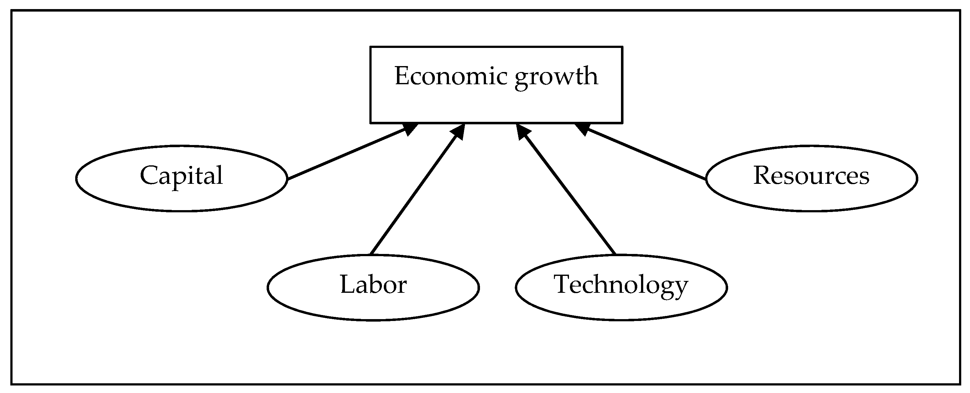
Factors driving economic growth include capital, labor, technology, and natural resources (Figure 1). Natural resources refer to the materials that human beings can directly obtain from nature and use for production and living. They mainly include land resources, water resources, climate resources, biological resources, mineral resources and energy [22]. Natural resources are the material basis of economic development [6]. The unsustainable use of natural resources is closely related to the principles or principles followed in the course of human economic activities [7]. The specific way of combining human and natural resources fundamentally determines the specific path of social and economic development.

2.1. Economic Growth Theory Ignores the Contribution of Natural Resources

In economic growth theory, economic growth is generally considered to be just a function of capital, technology, employment, etc. Resources are often be replaced by each other or by “other factors of production”. Adam Smith [23] believes that the core role in wealth growth is the improvement of “labor productivity”, which is mainly achieved through: the improvement of human skills and tools, the accumulation of capital, and the system. Ricardo [24] believes that a reasonable distribution system and incentives can increase people’s enthusiasm for production, and then promote economic growth. Marshall [25] emphasized the role of capital accumulation, investment, and entrepreneurial management activities in promoting economic growth. Keynes [26] analyzed the reasons for economic growth from a macro perspective, and he believes that by stimulating effective consumer demand and investment demand, economic growth can be promoted. Solow [27] developed a neo-classical economic growth model, arguing that long-term economic growth comes from technological progress. From classical economics to neoclassical economics, from neoclassical economic growth theory to endogenous growth theory, it can be seen that resources are not considered as the determinants of economic growth, and can always be replaced.

The theory of economic growth translates the “resource problem” into a simple “production cost problem”, and regards natural resources as “independent production factors” extracted from nature. For economic development, the reduction in the amount of resources is only a matter of increasing costs. The fact is that resources are used as factors of production to promote economic growth. Water resources, as basic natural resources and strategic economic resources, are the irreplaceable and indispensable core elements of productivity of human economic and social development [6,7].

2.2. Sustainable Economic Growth Must Consider Natural Resource Constraints

When the amount of resources is decreasing, people have begun to realize that resources will be the limiting factors of economic growth and development, seeing the limits of growth and development, and also causing theoretical debates about the limits of growth [28]. Due to changes in quantity, the overall characteristics of natural resources in the ecosystem will also change accordingly, which will affect the structure and function of the natural resource system in which they are located. Due to the mutual restraint relationship, the natural environment system in which the economic system is located has changed and become fragile, which further shakes the foundation of the entire economic growth [29]. Therefore, starting from the resources themselves, economic growth is limited by natural resources. The new growth theory proposes that for any country or region, it is inevitable to consume resources in the process of economic growth [8]. Due to the limitation of resources, the economic growth rate will be lowered to a certain extent than the growth rate without resource constraints. This reduction is called “drag effect” of resources on economic growth [8]. With the rapid economic development and increasing population, the supply and demand relationship of water resources is mostly unstable [5]. Water resources are limited, and the contradiction between supply and demand is growing due to the increasing demand of economic growth [6]. In addition, the problem of water pollution is becoming more and more serious, resulting in a serious shortage of water resources, which has become a bottleneck restricting social and economic development [20]. However, economic growth also provides conditions for investment in water development and utilization and governance, which is related to the pattern of water resources development, utilization and management [17].

In view of this, this paper considers the interaction between water resources and the socio-economic composite system in a coordinated manner, and studies the drag effect of water resources on economic growth and its changing trends deeply. So as to provide theoretical basis for the development and utilization of water resources and socio-economic development.

3. Model and Data

3.1. Improved Solow Growth Model

The classic model for measuring economic growth is the Solow Growth Model [8]. It has four main variables, namely, the output (Y), capital (K), labor (L) and “knowledge or labor validity” (A). The production function expression is as follows:

$$\mathrm{Y}\left(\mathrm{t}\right)=\mathrm{F}\left[\mathrm{K}\left(\mathrm{t}\right),\mathrm{A}\left(\mathrm{t}\right)\mathrm{L}\left(\mathrm{t}\right)\right]$$

(1)

This paper analyzes the drag effect of water resources on China’s economic growth, following Romer’s [8] Cobb–Douglas production function. Equation (1) becomes:

$$\mathrm{Yt}=\mathrm{K}{\left(\mathrm{t}\right)}^{\mathsf{\alpha }}\mathrm{W}{\left(\mathrm{t}\right)}^{\mathsf{\beta }}{\left[\mathrm{A}\left(\mathrm{t}\right)\mathrm{L}\left(\mathrm{t}\right)\right]}^{1-\mathsf{\alpha }-\mathsf{\beta }},(\mathsf{\alpha }>0,\mathsf{\beta }>0,\mathsf{\alpha }+\mathsf{\beta }<1)$$

(2)

where the dependent variable Y is the economic output, and the independent variables are K(t), W(t) and A(t)L(t), which indicate the fixed capital stock, water resources and labor force. α is the elasticity of the capital production, β is the elasticity of the water resources [8].

Taking the natural logarithm of both sides of Equation (2), the following can be obtained:

$$\ln \mathrm{Yt}=\mathsf{\alpha }\ln \mathrm{K}\left(\mathrm{t}\right)+\mathsf{\beta }\ln \mathrm{W}\left(\mathrm{t}\right)+\left(1-\mathsf{\alpha }-\mathsf{\beta }\right)\left[\ln \mathrm{A}\left(\mathrm{t}\right)+\ln \mathrm{L}\left(\mathrm{t}\right)\right]$$

(3)

Hence, the growth rate can be represented by Equation (4), after taking time as a derivative on both sides of Equation (3), as follows [30,31]:

$${\mathrm{g}}_{\mathrm{Y}}\left(\mathrm{t}\right)={\mathsf{\alpha }\mathrm{g}}_{\mathrm{K}}\left(\mathrm{t}\right)+{\mathsf{\beta }\mathrm{g}}_{\mathrm{W}}\left(\mathrm{t}\right)+\left(1-\mathsf{\alpha }-\mathsf{\beta }\right)\left[{\mathrm{g}}_{\mathrm{A}}\left(\mathrm{t}\right)+{\mathrm{g}}_{\mathrm{L}}\left(\mathrm{t}\right)\right]$$

(4)

where ${\mathrm{g}}_{\mathrm{Y}}\left(\mathrm{t}\right)$, ${\mathrm{g}}_{\mathrm{K}}\left(\mathrm{t}\right)$, ${\mathrm{g}}_{\mathrm{W}}\left(\mathrm{t}\right)$, ${\mathrm{g}}_{\mathrm{A}}\left(\mathrm{t}\right)$, and ${\mathrm{g}}_{\mathrm{L}}\left(\mathrm{t}\right)$ represent the growth rates of Y, K, W, A, and L, respectively.

Assuming that labor, knowledge, water resources, and land all increase at a constant rate, the capital and output needed to balance the growth path increase at a constant rate [8]. The Equation for the motion of capital is $\dot{\mathrm{K}}\left(\mathrm{t}\right)=\mathrm{sY}\left(\mathrm{t}\right)-\mathsf{\delta }\mathrm{K}\left(\mathrm{t}\right)$, from which the growth rate of capital is:

$$\dot{\mathrm{K}}\left(\mathrm{t}\right)/\mathrm{K}\left(\mathrm{t}\right)=\mathrm{s}\left[\mathrm{Y}\left(\mathrm{t}\right)/\mathrm{K}\left(\mathrm{t}\right)\right]-\mathsf{\delta }$$

(5)

In order to keep the growth rate of K constant, Y/K must be constant; that is, the growth rates of Y and K must be equal. In addition, there is a balanced growth path, which is ${\mathrm{g}}_{\mathrm{Y}}\left(\mathrm{t}\right)={\mathrm{g}}_{\mathrm{K}}\left(\mathrm{t}\right)$ [8]. The growth rate of Y on the path of balanced economic growth under constraints can then be obtained [22,23]:

$$\mathrm{s}{\mathrm{g}}^{\mathrm{bgp}}{}_{\mathrm{Y}}=\left[{\mathsf{\beta }\mathrm{g}}_{\mathrm{W}}\left(\mathrm{t}\right)+\left(1-\mathsf{\alpha }-\mathsf{\beta }\right)\left(\mathrm{g}+\mathrm{n}\right)\right]/\left(1-\mathsf{\alpha }\right)$$

(6)

where ${\mathrm{g}}^{\mathrm{bgp}}{}_{\mathrm{Y}}$ represents the growth rate of Y on the balanced growth path, n represents the labor growth rate, and g represents the knowledge growth rate. From this, the average output growth rate of the unit labor force on the balanced growth path can be derived as:

$$\begin{array}{c}{\mathrm{g}}^{\mathrm{bgp}}{}_{\mathrm{Y}/\mathrm{L}}={\mathrm{g}}^{\mathrm{bgp}}{}_{\mathrm{Y}}-{\mathrm{g}}^{\mathrm{bgp}}{}_{\mathrm{L}}\\ =\left\{\left[{\mathsf{\beta }\mathrm{g}}_{\mathrm{W}}\left(\mathrm{t}\right)+\left(1-\mathsf{\alpha }-\mathsf{\beta }\right)\left(\mathrm{g}+\mathrm{n}\right)\right]/\left(1-\mathsf{\alpha }\right)\right\}-\mathrm{n}\\ =\left[\left(1-\mathsf{\alpha }-\mathsf{\beta }\right)\mathrm{g}+{\mathsf{\beta }\mathrm{g}}_{\mathrm{W}}\left(\mathrm{t}\right)-\mathsf{\beta }\mathrm{n}\right]/\left(1-\mathsf{\alpha }\right)\end{array}$$

(7)

The drag effect of water resources equals the value of water resources that are unconstrained, subtracting the value of the water resources that are constrained [30,31]. When water resources are unconstrained in economic growth and increase with the growth of labor, the growth rate of water resources is equal to the growth rate of labor (growth rate is n) [30,31]. When water resources are constrained, the growth rate of water resources is 0 [30,31]. Based on this:

$$\begin{array}{c}\begin{array}{ll}{\mathrm{Drag}}_{\mathrm{water}}& ={\tilde{\mathrm{g}}}^{\mathrm{bgp}}{}_{\mathrm{Y}/\mathrm{L}}-{\mathrm{g}}^{\mathrm{bgp}}{}_{\mathrm{Y}/\mathrm{L}}\\ & =\left[\left(1-\mathsf{\alpha }-\mathsf{\beta }\right)\mathrm{g}+\mathsf{\beta }\mathrm{n}-\mathsf{\beta }\mathrm{n}\right]/\left(1-\mathsf{\alpha }\right)-\left[\left(1-\mathsf{\alpha }-\mathsf{\beta }\right)\mathrm{g}+\mathsf{\beta }*0-\mathsf{\beta }\mathrm{n}\right]/\left(1-\mathsf{\alpha }\right)\end{array}\\ {\mathrm{Drag}}_{\mathrm{water}}=\mathsf{\beta }\mathrm{n}/\left(1-\mathsf{\alpha }\right)\end{array}$$

(8)

3.2. Virtual Water Model

At present, the internationally authoritative software for virtual water measurement is CROPWAT, as recommended by the UN Food and Agriculture Organization [17,18]. Therefore, this paper also uses CROPWAT software to calculate the virtual water content of China’s agricultural products. The CROPWAT software is a computer program, established by FAO for irrigation planning and management. The CROPWAT software is developed based on the revised Penman formula, which calculates the water demand of a reference crop based on the climate and soil parameters of each region [32]. For the benchmark, the Penman formula is used to correct the values based on different crop coefficients. The meteorological data, which are required by the CROPWAT software, are derived from FAO’s CLIMATAT database. The unit virtual water content of each crop can be calculated as follows:

$$\mathrm{SWD}=\mathrm{CWR}/\mathrm{CY}$$

(9)

where SWD is the virtual water content per unit weight of the crop (m³/kg); CWR is the water requirement per unit area of the crop (m³/hm²); and CY is the yield per unit area of the crop (kg/hm²). Additionally, the data of CY are obtained from the China Statistical Yearbook (1987–2017). The crop water requirement (CWR) can be obtained by calculating the amount of soil evaporation (${\mathrm{ET}}_{\mathrm{c}}$) accumulated during the whole growth period of the crop [32]:

$$\mathrm{CWR}=10\times {\displaystyle \sum }_{\mathrm{i}=1}^{\mathrm{nd}}{\mathrm{ET}}_{\mathrm{C}}=10\times {\mathrm{K}}_{\mathrm{c}}{\displaystyle \sum }_{\mathrm{i}=1}^{\mathrm{nd}}{\mathrm{ET}}_0$$

(10)

where ${\mathrm{ET}}_{\mathrm{c}}$ is the soil evaporation; ${\mathrm{ET}}_0$ is the daily potential evaporation (mm/d) during the crop growth period; ${\mathrm{K}}_{\mathrm{c}}$ is the corresponding crop coefficient; and nd is the total number of days in the crop growth period.

Using the meteorological data for each site in the CLIMWAT database to select the soil type of the study area, the value of ${\mathrm{ET}}_{\mathrm{c}}$ can be directly obtained using the CROPWAT software, and then the virtual water content per unit weight of the crop can be obtained using Equation (9). The Equation for calculating the total amount of crop virtual water is shown in Equation (11):

$$\mathrm{TVW}=\mathrm{SWD}\times \mathrm{TCY}$$

(11)

where TVW is the total amount of virtual water (t) of a crop; and TCY is the total yield (kg) of the crop in that year.

3.3. Study Area and Data Sources

In order to scientifically reflect the social and economic development of different regions of China, according to the criteria of the National Bureau of Statistics, China’s economic region is divided into the eastern region (Beijing, Tianjin, Hebei, Shanghai, Jiangsu, Zhejiang, Fujian, Guangdong, Shandong, and Hainan), western region (Neimenggu, Guangxi, Chongqing, Sichuan, Guizhou, Yunnan, Xizang, Shaanxi, Gansu, Qinghai, Ningxia, and Xinjiang), central region (Shanxi, Anhui, Jiangxi, Henan, Hubei, and Hunan) and the northeast region (Liaoning, Jilin, and Heilongjiang). Hong Kong, Macao and Taiwan are not within the scope of this study.

The main variables in this paper are the output (Y), water resources (W), labor force (L), and fixed capital stock (K). The selection criteria are listed in

Table 1. Variable Selection.

Variable	Variable Interpretation	References and Data Sources
Output	The economic output is expressed in terms of the gross domestic product (GDP), and the GDP is adjusted at a constant price based on the figures from 1978.	[6,30,31,33,34,35]
Labor force	The labor force is represented by the data on social workers at the end of the year in each region.	[20,30,31,33,34,35]
Water resources	The water resources are represented by the sum of the virtual agricultural water (water from agricultural products), consumption water (water for household use), industry water (water for industry use), and ecological water (water for ecological use), where virtual agricultural water is the sum of the calculated virtual water of crops and the virtual water of animal products.	[20,34,35]
Fixed capital stock	The fixed capital stock refers to the total amount of fixed capital in the economic society at a certain point in time. The fixed capital was calculated using a depreciation rate of 0.06 with the perpetual inventory method, and the fixed capital stock is adjusted at a constant price based on the figures from 1978.	[30,31,33,34,35]

.

The measurement results concerning the virtual water content of major agricultural product units (SWD) in various provinces of China are shown in

Table 2. Virtual water content of major agricultural product units in various provinces of China (unit: m³/kg).

Cities	Paddy	Wheat	Corn	Beans	Potato	Cotton	Oil	Hemp	Sugar Cane	Beet	Tobacco Leaf	Tea	Apple	Citrus	Pear	Grape	Banana
China	1.29	1.26	0.80	1.94	1.20	4.69	1.59	3.32	0.19	0.32	2.13	12.43	0.61	0.66	0.91	0.53	0.53
Beijing	1.25	0.95	0.73	2.22	0.88	5.34	2.25	5.07			4.83		0.84		0.67	0.60
Tianjin	1.05	0.74	0.75	2.29	0.65	3.18	1.14	5.46					0.49		0.54	0.20
Hebei	1.11	0.67	0.77	2.05	1.20	5.27	1.07	2.50		0.10	1.77		0.40		0.27	0.27
Shanxi	1.28	1.07	0.85	5.76	2.41	4.09	3.10	6.84		0.09	1.61	31.34	0.29		0.39	0.23
Neimenggu	1.76	1.21	0.64	2.65	1.61	3.67	1.77	1.80		0.11	1.11		0.84		0.57	0.40
Liaoning	1.10	1.11	0.75	1.98	0.34	4.38	1.73	4.60		0.11	4.27		0.47		0.65	0.25
Jilin	0.98	0.95	0.53	2.19	0.59	2.96	1.19	4.37		0.11	1.24		0.76		0.83	0.44
Heilongjiang	1.50	1.21	0.69	2.29	1.02		1.85	0.97		0.13	1.63		0.45		0.56	0.27
Shanghai	1.06	1.19	0.68	1.38	0.98	2.13	1.66	5.32	0.18					0.13	0.45	0.34
Jiangsu	0.97	0.89	0.71	1.09	0.73	4.98	1.11	2.05	0.15	0.33	1.81	18.34	0.42	0.53	0.38	0.28
Zhejiang	1.12	1.16	0.84	1.06	0.87	3.56	1.48	1.50	0.12		1.47	7.58		0.32	0.40	0.18
Anhui	1.26	0.88	0.79	2.59	2.16	6.03	1.23	1.86	0.26	0.12	1.51	12.12	0.30	0.98	0.28	0.22
Fujian	1.40	1.82	0.97	1.15	0.91	7.68	1.30	2.10	0.17		1.83	4.26		0.29	0.67	0.25	0.28
Jiangxi	1.64	2.86	1.11	1.78	1.08	4.72	2.30	4.38	0.24		1.96	11.85		0.68	1.40	0.58
Shandong	0.95	0.75	0.64	1.31	0.61	4.70	0.81	3.04		0.19	1.49	6.77	0.21		0.25	0.17
Henan	1.38	0.90	0.94	2.37	1.78	6.90	1.17	1.07	0.17		2.09	17.00	0.34	2.41	0.45	0.32
Hubei	1.16	1.39	1.00	1.47	1.72	7.10	1.71	2.58	0.27	0.95	2.16	6.65	0.96	0.41	0.56	0.26
Hunan	1.27	1.34	0.81	1.27	1.10	5.32	2.16	2.70	0.20		1.78	5.06		0.55	1.70	0.73
Guangdong	1.23	1.49	0.82	1.12	0.86		1.02	2.23	0.12		1.43	4.71	0.49	0.43	1.00		0.30
Guangxi	1.57	3.00	0.95	2.00	1.78	5.77	1.40	2.30	0.14		2.36	8.57		0.56	0.57	0.37	0.39
Hainan	2.37		1.12	1.50	1.33		1.44	1.05	0.21		7.93	14.70		1.10			0.38
Chongqing	0.97	1.31	0.71	1.35	1.06	8.22	1.67	3.31	0.20		1.83	5.84	0.98	0.52	0.59	0.39	0.39
Sichuan	0.73	0.90	0.56	1.01	0.87	3.81	1.11	2.32	0.17	0.63	1.34	5.81	0.32	0.38	0.42	0.30	0.34
Guizhou	1.24	1.18	0.84	2.11	1.28	4.67	1.72	2.95	0.15	1.25	1.93	12.51	1.40	1.05	1.05	0.57	1.70
Yunnan	1.05	1.43	0.58	0.99	1.16	3.23	1.32	3.71	0.16	0.29	1.31	8.56	0.82	0.71	0.70	0.15	0.47
Xizang	1.99	0.98	0.94	0.92	0.81		1.34							0.68	0.50
Shaanxi	1.17	1.05	0.98	1.75	1.95	2.05	1.90	4.47	0.36	0.57	2.25	11.49	0.43	0.39	0.35	0.36
Gansu	1.56	1.18	0.80	2.11	0.60	3.88	1.71	3.92		0.09	1.39	43.04	0.57	0.38	0.64	0.45
Qinghai		1.44	0.72	1.43	1.41		1.97	7.19		0.21	1.00		1.30		9.37	4.82
Ningxia	0.88	1.71	0.64	5.58	2.43		2.00	5.62		0.29	1.18		0.54		0.55	0.98
Xinjiang	1.79	0.99	0.81	1.33	0.99	3.70	1.72	2.29		0.10	3.09		0.44		0.45	0.34

and

Table 3. Animal product quality virtual water content (unit: m³/kg).

	Pork	Beef	Lamb	Milk	Egg	Aquatic Products
Virtual water	2.522	12.596	5.948	5.982	6.165	5.000

(the blank in the table indicates that the crop is not grown in the area).

4. Results and Analysis

4.1. Data Stationarity and Cointegration Test

This paper uses a panel data model to analyze the drag effect of water resources in the four major economic zones (East, Central, West, and Northeast China) based on data from 1987 to 2017 for 31 provinces (municipalities and autonomous regions). The stability and co-integration of the data will have an impact on the analysis of the drag effect of economic growth [3,8,20,21]. At the same time, due to the two-dimensional nature of the panel data, the stability of the data directly determines the credibility of the results, so a panel data model is adopted. Before the regression analysis, the data should be tested for stationarity and co-integration. The most common method is the unit root test [8,20,21]. In this paper, two-unit root test methods are used, the same-root LLC (Levin–Lin–Chu) test and different-root Fisher-ADF test. If the hypothesis of the existence of a unit root is rejected in both tests, the data is considered to be stationary. If the hypothesis of the existence of a unit root is accepted, the data is considered to be unstable.

Based on formula 3, the logarithms of GDP, Water, Labor, and Capital are calculated—$\ln \mathrm{Y}\left(\mathrm{t}\right)$, $\ln \mathrm{W}\left(\mathrm{t}\right)$, $\ln \mathrm{L}\left(\mathrm{t}\right)$, and $\ln \mathrm{K}\left(\mathrm{t}\right)$, respectively. The unit root tests were performed using STATA software. By testing the first-order difference values of $\ln \mathrm{Y}\left(\mathrm{t}\right)$, $\ln \mathrm{W}\left(\mathrm{t}\right)$, $\ln \mathrm{L}\left(\mathrm{t}\right)$, and $\ln \mathrm{K}\left(\mathrm{t}\right)$, it is found that there are no unit roots at the significance level of 1%, indicating that these four variables are all first-order single integer I (1) (

Table A1. Unit root test results.

Regions		LLC Test	Fisher-ADF Test
		Adjusted t	Inverse chi-squared	Inverse normal	Inverse logit t	Modified inv. chi-squared
Eastern Region	LnY(t)	−2.3614 ***	58.1872 ***	−4.5777 ***	−4.8404 ***	6.0379 ***
	LnL(t)	−6.8928 ***	55.2886 ***	−4.1441 ***	−4.4513 ***	5.5796 ***
	LnW(t)	−16.4979 ***	55.5169 ***	−4.5330 ***	−4.6324 ***	5.6157 ***
	LnK(t)	−2.1354 **	62.8900 ***	−5.0898 ***	−5.3508 ***	6.7815 ***
Western Region	LnY(t)	−3.7450 ***	70.1643 ***	−4.8760 ***	−5.0960 ***	6.6632 ***
	LnL(t)	−9.2896 ***	53.9717 ***	−3.9194 ***	−3.8922 ***	4.3260 ***
	LnW(t)	−15.3768 ***	62.7292 ***	−4.7308 ***	−4.7477 ***	5.5901 ***
	LnK(t)	−2.3007 **	60.9894 ***	−4.5402 ***	−4.5705 ***	5.339 ***
Central Region	LnY(t)	−1.4489 **	32.8865 ***	−3.4768 ***	−3.5722 ***	4.2634 ***
	LnL(t)	−6.6827 ***	29.9360 ***	−2.6454 ***	−2.7659 ***	3.6612 ***
	LnW(t)	−16.8324 ***	33.5124 ***	−3.3366 ***	−3.5270 ***	4.3912 ***
	LnK(t)	−2.1286 **	32.0596 ***	−3.4153 ***	−3.4867 ***	4.0946 ***
Northeast Region	LnY(t)	−5.1730 ***	14.3247 **	−2.0435 **	−2.1126 **	2.4031 ***
	LnL(t)	−2.6477 ***	15.1747 **	−2.2596 **	−2.3185 **	2.6485 ***
	LnW(t)	−5.9413 ***	14.5111 **	−2.3115 **	−2.2761 **	2.4570 ***
	LnK(t)	−2.1952 **	20.2018 ***	−2.6094 ***	−3.0787 ***	4.0997 ***
Entire Country	LnY(t)	−5.1558 ***	154.1801 ***	−6.9654 ***	−7.0112 ***	8.278 ***
	LnL(t)	−13.8978 ***	145.2444 ***	−6.3203 ***	−6.2978 ***	7.4756 ***
	LnW(t)	−23.9241 ***	152.1200 ***	−7.0760 ***	−7.0231 ***	8.0930 ***
	LnK(t)	−2.8927 ***	162.3613 ***	−7.4548 ***	−7.5328 ***	9.0127 ***

***, ** and *, respectively, represent that the significant is under the level of 1, 5 and 10%. The same below.

).

Co-integration refers to the sequence of a linear combination of two or more non-stationary variables; that is, the sequence of these variables has a long-term equilibrium co-integration relationship [8,20,21]. The unit root test results show that the variables are the same order and single, so the co-integration test can be performed. Through the data stability and co-integration tests, it is found that $\ln \mathrm{Y}\left(\mathrm{t}\right)$, $\ln \mathrm{W}\left(\mathrm{t}\right)$, $\ln \mathrm{L}\left(\mathrm{t}\right)$, and $\ln \mathrm{K}\left(\mathrm{t}\right)$ are an unstable sequence (

Table A2. Co−integration test results.

Regions	Kao Test			Pedroni Test
	Modified Dickey-Fuller	Dickey-Fuller	Augmented Dickey-Fuller	Modified Phillips-Perron	Phillips-Perron	Augmented Dickey-Fuller
Eastern Region	−4.5345 ***	−5.3641 ***	−6.5600 ***	0.9164	−1.9340 **	−3.1989 ***
Western Region	−7.2003 ***	−5.7966 ***	−5.2559 ***	0.1312	−5.9060 ***	−4.4322 ***
Central Region	−4.8577 ***	−4.0680 ***	−5.7364 ***	1.9139 **	−0.3784	−1.5683 **
Northeast Region	−2.1379 ***	−2.8561 ***	−4.3306 ***	0.7748	−1.2143	−2.5258 **
Entire Country	−8.5806 ***	−8.8069 ***	−10.9698 ***	0.9116	−5.4188 ***	−6.0502 ***

). However, there is at least one co-integration relationship between them, indicating that there is a long-term stable equilibrium relationship between the variables, and the regression residuals of the equations are stable. Therefore, further regression analysis can be done.

4.2. Analysis of the Spatial Dimension of the Drag Effect of Water Resources

According Equation (8), ${\mathrm{Drag}}_{\mathrm{water}}=\mathsf{\beta }\mathrm{n}/\left(1-\mathsf{\alpha }\right)$. α is the elasticity coefficient of the capital, β is the elasticity coefficient of the water resources, n is the labor growth rate. Based on the results of Variable coefficient panel model in

Table 4. Variable coefficient panel model and “Drag” measurement results for China’s 31 provinces.

Cities and Regions	Water	Capital	Labor	N-GDP	N-Capital	N-Labor	N-Water	D-Water
Entire Country	0.06	0.42	0.07	11.11	13.11	1.54	3.06	0.1478
Beijing	0.02	0.19	0.11	10.03	11.22	2.58	1.38	0.0596
Tianjin	0.10	0.63	0.01	11.72	12.92	2.21	3.78	0.6198
Hebei	0.12	0.44	0.41	10.77	13.28	1.48	4.65	0.3269
Shanghai	0.01	0.50	0.01	10.18	10.91	1.86	−0.25	0.0420
Jiangsu	0.07	0.95	−0.14	12.04	14.74	1.10	2.00	1.4693
Zhejiang	0.06	0.90	0.12	12.28	13.90	0.86	1.42	0.5024
Fujian	0.25	0.29	0.35	12.34	14.10	2.77	2.84	0.9762
Shandong	0.19	0.67	0.17	11.65	13.22	1.92	3.78	1.1040
Guangdong	−0.03	0.76	0.73	13.35	14.54	2.63	1.65	−0.3364
Hainan	0.03	0.52	0.07	10.99	12.83	2.47	6.63	0.1603
Eastern Region	0.05	0.61	0.06	11.80	13.47	1.83	2.69	0.2316
Neimenggu	0.07	0.52	−0.07	11.98	16.72	1.58	6.56	0.2249
Guangxi	0.07	0.30	0.35	10.68	13.74	1.24	2.37	0.1201
Chongqing	0.01	0.58	0.68	11.68	14.09	0.43	4.70	0.0128
Sichuan	−0.03	0.49	0.60	10.53	10.73	0.69	1.40	−0.0350
Guizhou	−0.01	0.29	−0.22	10.15	11.80	1.15	2.82	−0.0092
Yunnan	0.02	0.21	0.40	10.13	14.09	1.82	4.30	0.0450
Xizang	0.05	0.37	0.10	11.29	13.27	3.16	3.52	0.2650
Shaanxi	0.05	0.55	0.39	11.04	12.63	1.20	3.22	0.1270
Gansu	0.04	0.25	0.06	10.00	11.61	1.06	3.04	0.0622
Qinghai	−0.02	0.31	0.01	9.60	13.13	1.76	1.99	−0.0586
Ningxia	0.06	0.24	−0.05	9.81	12.54	2.29	6.79	0.1772
Xinjiang	0.01	0.20	0.09	9.71	13.26	2.78	5.48	0.0506
Western Region	0.04	0.34	0.05	10.72	13.06	1.22	3.45	0.0741
Shanxi	0.12	0.29	−0.05	9.78	10.82	1.50	3.40	0.2430
Anhui	0.18	0.52	0.29	10.93	11.87	1.80	2.12	0.6814
Jiangxi	0.06	0.36	−0.10	10.49	13.11	1.64	2.45	0.1490
Henan	0.11	0.31	−0.25	10.73	14.32	1.98	3.72	0.3202
Hubei	0.21	0.50	−0.08	10.87	13.58	1.44	2.32	0.5960
Hunan	0.02	0.45	0.45	10.34	11.86	0.95	2.00	0.0385
Central Region	0.17	0.37	−0.13	10.61	12.98	1.60	2.62	0.4341
Liaoning	−0.01	0.52	0.26	9.13	11.52	0.59	4.84	−0.0075
Jilin	0.03	0.44	−0.02	10.02	13.70	1.30	3.47	0.0587
Heilongjiang	0.05	0.35	0.18	8.98	9.99	1.59	5.08	0.1251
Northeast Region	0.04	0.46	0.15	9.28	11.65	1.11	4.64	0.0863

“Water” is the elasticity coefficient of water resources; “Capital” is the elasticity coefficient of capital; “Labor” is the elasticity coefficient of labor; “N-GDP” is the growth rate of GDP; “N-Capital” is the growth rate of capital; “N-Labor” is the growth rate of labor; “N-Water” is the growth rate of water resources; and “D-Water” is the “Growth Drag” of water resources. N-GDP; N-Capital; N-Labor; N-Water; D-Water; unit: %. The same abbreviation definitions apply to the table below.

, we can get the second column (Water) is equal to β, the third column (Capital) is equal to α, and the seventh column (N-Labor) is equal to n. Therefore, we can get the growth drag of water resources, and the results is in the ninth column (D-Water).

Under water resource constraints, China’s overall economic growth rate dropped by 0.15%. The average annual growth rate of the eastern, western, central and northeastern regions declined by 0.23%, 0.07%, 0.43%, and 0.09% (Table 4). That is to say, the economic growth of the central region is more affected by water resources, followed by the east, west and northeast. It can be seen that the drag effect of water resources on the central region, which is affected by rapid economic growth (a GDP growth rate of 10.61%), cannot be ignored. Water resources constrain the economic growth of the central region at a rate of 0.43% per year. If this rate continues, the economic growth rate in the central region will be reduced to 91.34% in 2040. From the perspective of regional characteristics, Henan Province in the central region is a large grain province, and Hunan Province is a land of rice. The economic growth of these provinces is highly dependent on water resources, so there is a large water drag effect on the economic growth of the central region. The eastern region is a coastal city with a developed aquaculture industry and a high degree of dependence on water resources. Therefore, the economic growth of the region is also constrained by there being less available water. The economic growth of the western and northeastern regions is less constrained by water resources, which is mainly related to the development direction of the region. The economic growth in the northeast region mainly relies on the development of energy, such as oil and coal. The labor force growth rate in the western region is small (1.22%), and the capital stock accumulation rate is relatively fast (13.06%). The economic growth is mainly related to the accumulation of capital stock and has little dependence on water resources. Therefore, the water resources efficiency of the economic growth in the western region is lower than that in other parts of the country.

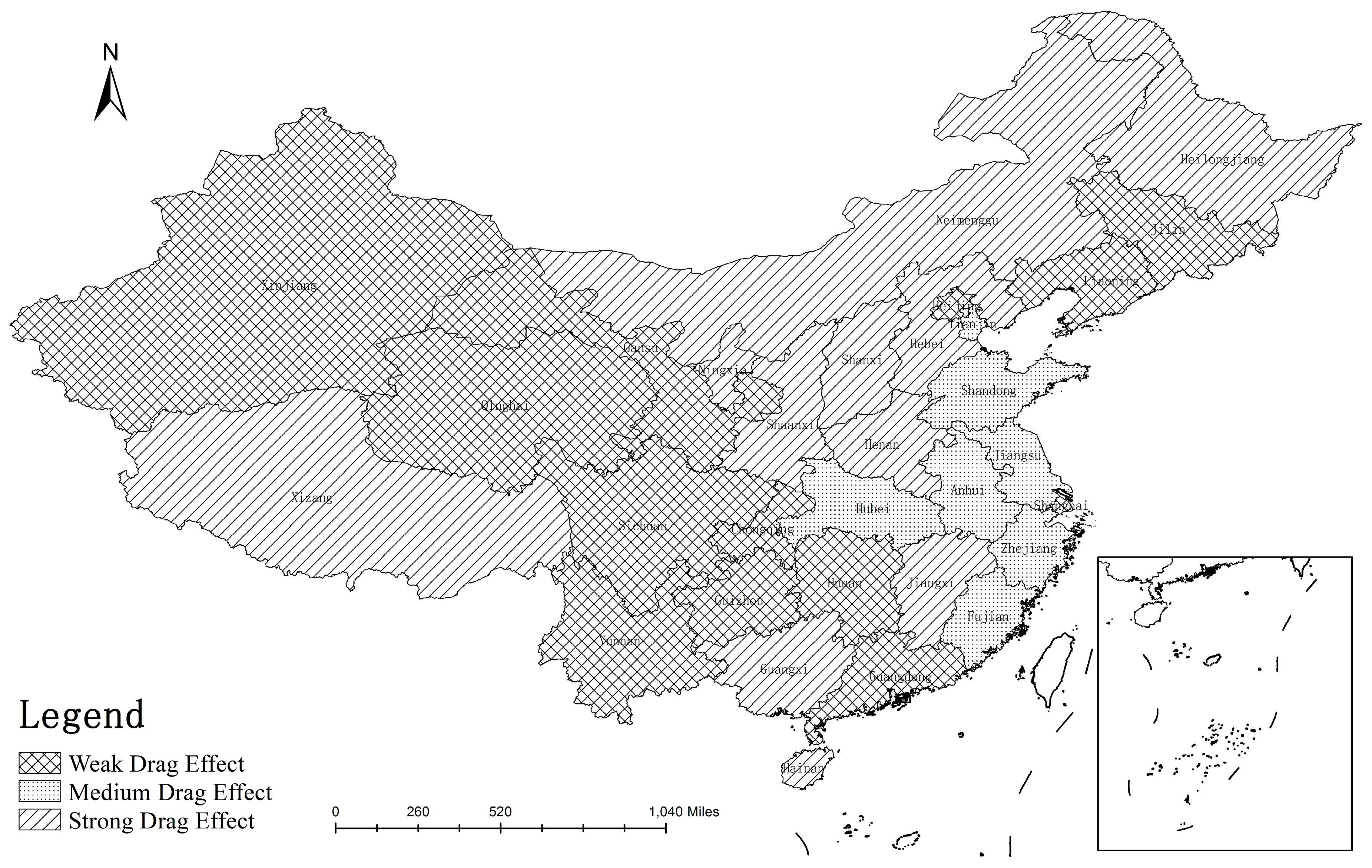
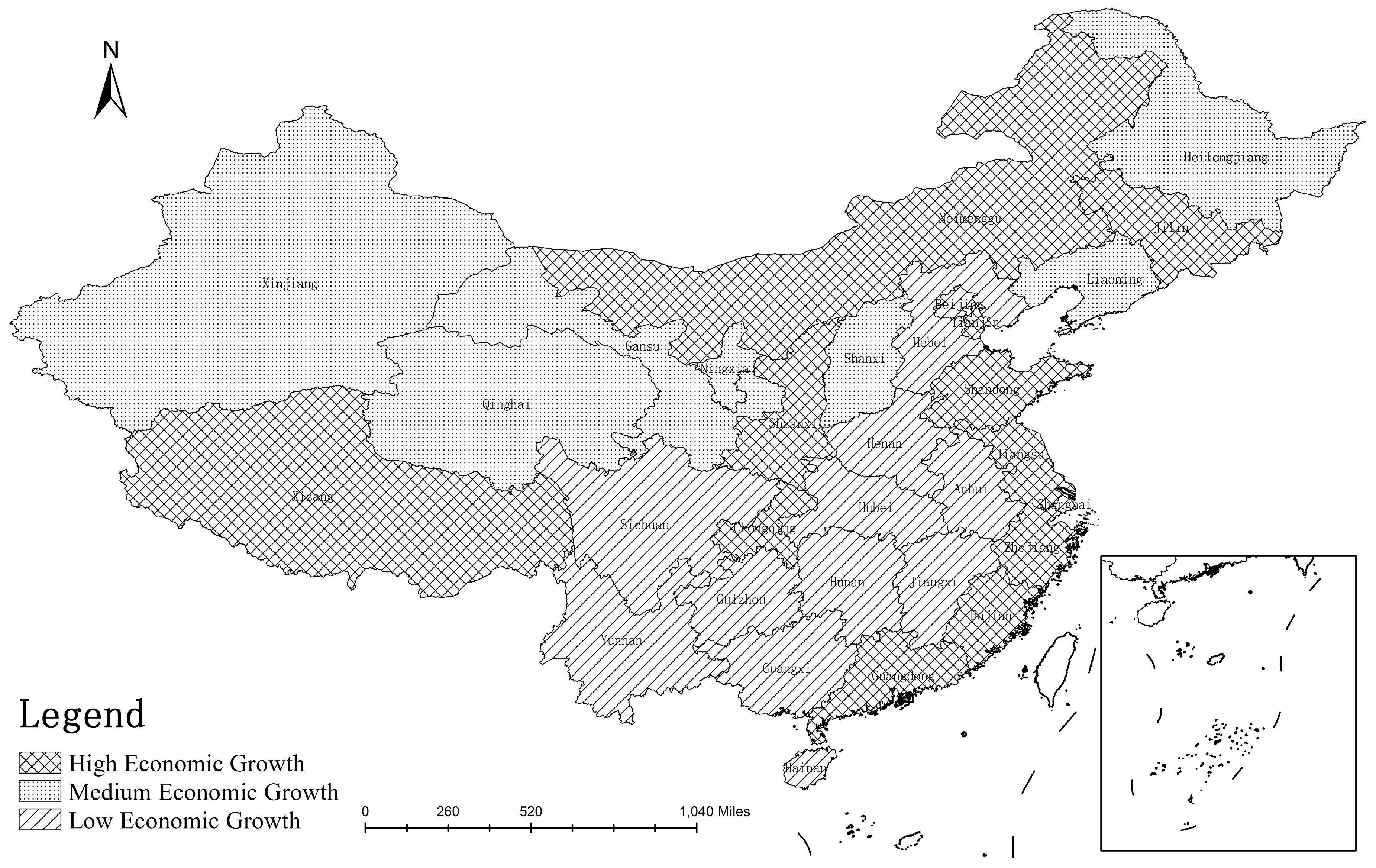
There is a large regional imbalance in China’s water resources, and there are also serious regional imbalances in economic growth [36]. Therefore, there are also differences in resource constraints to economic growth in different regions. In order to more fully reveal the impact of water resources in different regions of China on the economic growth of the region, this paper conducts regression analysis on 31 provinces and cities, based on panel data from 1987 to 2017 (Table 4). At the same time, according to the size of D-Water and N-GDP, 31 provinces and cities are divided into weak, medium and strong, which constitute three “Growth Drag” constraint levels (Figure 2), and low, medium and high, which constitute three economic growth types (Figure 3).

The drag effect of water resources in Beijing, Gansu and other provinces are weakly constrained. There are two main reasons for why water resources are less constrained by the economic growth of these provinces: the economic growth rate of provinces, such as Beijing, Shanghai, and Chongqing, ranks in the top 10 in the country, the labor growth rate is medium-speed, and the accumulation of capital stock is fast, indicating that it is local. The greater degree of economic growth is related to the accumulation of capital, so water resources are relatively less restrictive to these areas. In the central and western regions of Hunan and Gansu, the economic growth rate is slow, and the labor growth rate is lower than the national average. The current situation of sparsely populated land has largely alleviated the pressure of water resources on economic growth.

The water resources of Hebei, Shaanxi, Henan and other provinces have moderate constraints on the economy. The reasons are mainly divided into two categories: In Tibet, Guangxi, Henan and other large and medium-sized land areas, the capital stock growth rate is higher than 13.5%, and the labor growth rate is higher than 1.20%. The high-speed accumulated capital and increasing labor force have led to an increasing demand for water resources in these areas, which has led to a moderate constraint on water resources growth. Hainan and Hebei have developed coastal cities with a medium-speed growth. The growth rate of the labor force is remarkable, and the increasing demand for water resources by the labor force is also increasing. Therefore, the water resources in these areas have a moderate constraint on economic growth.

Water resources are strongly constrained in economically developed areas, such as Tianjin and Jiangsu, mainly because the region attracts a large amount of high-quality labor, resulting in an increase in the labor growth rate. At the same time, the demand for water resources in aquaculture and high-speed industries is increasing, so water resources have created strong constraints on the fast-growing economy of the region. There are two main reasons for the strong constraints on the economic growth of Anhui and Hubei. On the one hand, the fast-growing agriculture in these two provinces is heavily dependent on water resources. At the same time, these areas have a large area, but the available water resources are limited. Therefore, the per capita water resources are low, which leads to the drag effect of water resources on economic growth being higher than that in other provinces. On the other hand, the elasticity coefficient of water resources in these areas is greater than that in most provinces, that is, the contribution of water resources to economic growth is very high. In the case of low water resources, a high dependence on water resources has a strong constraint on economic growth.

4.3. Analysis of the Temporal Dimensions of the Drag Effect of Water Resources

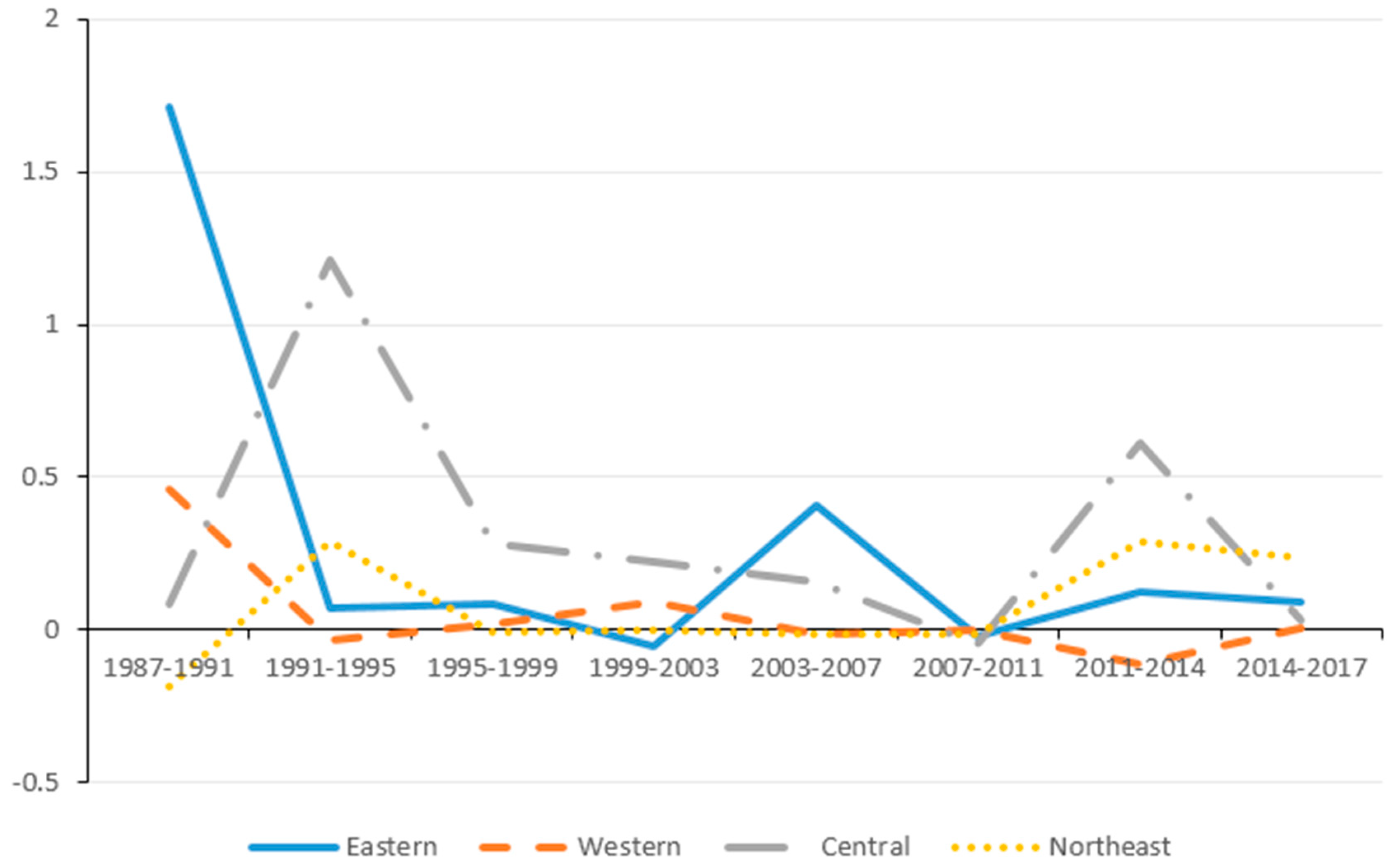
Economic growth is a dynamic process, and the impact of water resources on economic growth is also a dynamic process. In order to further study the impact degree and dynamic change process of water resources in regional economic growth, this paper uses the time variation method of the panel data to examine the changes of the drag effect of water resources on China’s eastern, western, central and northeastern regions from 1987–2017 (Figure 4,

Table A3. Drag effect of water resources and policies of water project.

Drag and Water Projects		1987–1991	1991–1995	1995–1999	1999–2003	2003–2007	2007–2011	2011–2014	2014–2017
D-Water	Eastern	1.7095	0.0726	0.0846	−0.0575	0.4065	−0.0244	0.1210	0.0890
	Western	0.4622	−0.0347	0.0200	0.0881	−0.0179	−0.0051	−0.1112	0.0049
	Central	0.0809	1.2132	0.2783	0.2247	0.1537	−0.0501	0.6112	0.0299
	Northeast	−0.1849	0.2862	−0.0070	−0.0034	−0.0168	−0.0156	0.2909	0.2376
Policies of Water Project	Project 1	Water Diversion Project from Luanhe River to Tianji City (Run since 1983)
	Project 2	Water Diversion Project from Luanhe River to Tangshan City (Run since 1984)
	Project 3	Water Diversion Project from Yellow River to Qingdao City (Run since 1986)
	Project 4	Water Diversion Project from Datong River to Qinwangchuan (Run since 1994)
	Project 5	East Line Project of South-to-North Water Diversion (Run since 2012)
	Project 6	Central Line Project of South-to-North Water Diversion (Run since 2014)

).

4.3.1. Analysis of the Drag Effect in the Eastern Region of China

From 1991 to 1999, the economic growth rate and the accumulation rate of fixed capital in the eastern region were the fastest in the past 30 years (averages of 16.81% and 15.04%, respectively). A large influx of labor and rapid capital accumulation caused the demand for resources to increase rapidly. The drag effect of water resources on economic growth became greater. During the period of 1999–2003, the strategy of developing the western region introduced water resources from the central and western regions into the eastern region, which alleviated the restrictions on water resource growth in the eastern region to some extent. Between 1987 and 2017, the economic growth in the eastern region consistently ranked first in the country. The water-end effect of economic growth in the region presents the dynamic characteristics of “obstruction–promotion–obstruction–promotion–obstruction” and gradually approaches a zero value, indicating that the dependence of economic growth on water resources in the eastern region is gradually decreasing. The slowdown in regional agricultural development is mainly related to the transformation of the economy by means of technological progress and capital accumulation. It shows that the economy of the eastern region is gradually entering a stage of sustainable development.

4.3.2. Analysis of the Drag Effect in the Western Region of China

Between 1987 and 2017, the trend of water resources in the western region on economic growth was “obstruction–promotion–obstruction–promotion–obstruction”. Since 2000, China has implemented the strategy of developing the western region. This policy has also accelerated the economic growth of the western region. At the same time, it has also attracted some labor backflow. The return of labor to drive production and living in the western region has increased the demand for water resources, further leading to water shortages. The water resources drag effect became larger. To achieve sustainable development in the western region, it is necessary to optimize the industrial structure, improve technical efficiency, promote the development of green agriculture, reduce the dependence of economic development on water resources, and gradually achieve sustainable economic development.

4.3.3. Analysis of the Drag Effect in the Central Region of China

Between 1987 and 2017, the drag effect of water resources in the central region was second only to that of the eastern region. The main reasons are as follows: First, the labor growth rate in the central region has been declining year-by-year, and the situation of labor loss in the eastern region is more serious. The demand for water resources is reduced. Second, the growth rate of capital stock is “growth-decrease-growth-decrease”, which is basically consistent with the law of economic growth, indicating that economic growth in the central region is mainly related to the accumulation of capital. Third, the growth rate of water consumption in the central region of each period is greater than that of other regions, that is, its economic growth relies heavily on water resources. Fourth, water resources have always imposed constraints on economic growth in the central region and particularly in Henan and Hunan. The agricultural development of Shanxi and other provinces is mainly dependent on water resources. Therefore, water resources have a continuous drag effect on the economic growth of the central region. In response to this problem, the central region should promote water-saving irrigation technology, improve the efficiency of agricultural technology, and reduce the constraints of water resources on economic growth.

4.3.4. Analysis of the Drag Effect in the Northeast Region of China

Between 1987 and 2017, the drag effect of water resources in Northeast China gradually increased. The main reasons are as follows: First, it is related to the industrial layout of the Northeast. From 1987 to 2007, the exploitation of oil fields and coal mines in the three provinces constituted the main economic growth initiatives. Since 2010, the state has gradually controlled the development of small coal mines in the northeast region, banned some small coal mines, transformed the industry in the northeast region, and rapidly developed ice and snow tourism. Therefore, the drag effect of water resources on economic growth in Northeast China during 2012–2017 declined. Second, after 2000, the labor force increased year-by-year, and capital stock was rapidly accumulated. The demand for water resources for living production in Northeast China has been increasing, making the consumption rate of water resources significantly higher than that in other regions, further leading to water resource constraints in the northeast region. The dependence is much higher than that in other regions.

5. Conclusions and Discussions

5.1. Conclusions

According to Romer’s [8] hypothesis, it is inevitable to consume resources in the process of economic growth. Due to the limitation of resources, the economic growth rate will be lowered to a certain extent than the growth rate without resource constraints. Therefore, this paper uses panel data to calculate both the time and space dimensions of the drag effect of water resources on China’s economic growth. By measuring the drag effect of water resources on different regions, we can compare and analyze the dependence of the economic growth of different regions on water resources. By analyzing the trends of the drag effect of water resources in different regions from 1987 to 2017, corresponding policy recommendations can be proposed for different regions. This paper aims to answer questions relating to China’s economic growth under water resource constraints and provide empirical evidence for governments at all levels to formulate relevant policies, with a view to promoting the stable, sustainable development of the Chinese economy and achieving minimum water resource constraints.

This paper studies the drag effect of water resources on the economic growth of China’s eastern, western, central and northeastern regions. Find and answer the questions from the beginning of the article. (1) Water resources have certain constraints on the economic growth of each region. And regional economic growth has declined by 0.23% (eastern), 0.07% (western), 0.43% (central), and 0.09% (northeastern) annually. (2) In provinces with rapid labor growth, water resources have a greater impact on economic growth (for example, in Fujian, Tianjin, etc.). In provinces with low labor growth rates, the drag effect of water resources on economic growth is affected by the capital stock of the region. In provinces with fast capital stock growth (for example, in Zhejiang and Guangxi), the water resources have a great drag effect on economic growth. In provinces with low capital stock growth (for example, in Sichuan, Guizhou, etc.), the water resources have a low drag effect on economic growth. (3) Through the analysis of the water drag effect of different time periods, this paper finds that the drag effect of water resources in different regions has changed a lot in different periods. The change in the drag effect in different periods have a certain relationship with the implementation of policies in this period. In some periods, the government’s mobilization of water resources for economic growth in some regions will not only promote the transfer of labor between regions, but also cause changes in the regional water resources.

5.2. Discussions

According to the results provided in this paper, only under the conditions of good government supervision, a reasonable allocation of existing water resources, the simultaneous strengthening of physical and human capital inputs for growth, and other aspects can the water resources have a good role in promoting economic growth. Therefore, in order to achieve the coordinated development of water resources and economic growth, future macro policies should focus on:

(1) For the provinces with strongly water resources constraints (such as Jiangsu and Shandong, etc.), as the population of these provinces continues to grow, and the size of cities continues to expand, water resources will constraint economic growth more and more. It is necessary to vigorously develop water-saving agriculture, improve technical efficiency, and reduce the strong dependence of economic growth on water resources. To further utilize internal and external resources to ease water resource constraints by adjusting the market.

(2) Provinces with moderate water resources constraints (such as Hebei, Shaanxi, etc.) have relatively low economic growth rates, but the rate of water consumption is far above the national average. These provinces should take the lead in deploying strategic emerging industries, and accelerate the development of the tertiary industry to reduce water consumption. So as to achieve the goal of reducing the drag effect of water resources on economic growth.

(3) Provinces with weakly water resources constraints (such as Guangdong, Qinghai, etc.) are mostly located in coastal water-rich areas. The labor growth rate in these provinces is low, but the capital stock is growing faster, so these provinces can promote the development of capital-based industries. Not only can the development of the economy be rational, but it can also reduce the economy’s dependence on water resources, thereby achieving the sustainable use of water resources and sustainable economic growth.

In this paper, the evaluation of the “growth drag effect” of regional water resources is only a preliminary study, and there are some problems that must be considered in further research: (1) Water resources are the premise and foundation of economic growth. The difference in water resource endowment determines the direction of regional economic growth and its development speed. At the same time, regional economic growth is a dynamic process. The drag effect of water resources in different regions varies greatly with time, and the water elasticity coefficient, capital elasticity coefficient and labor growth rate affect the drag effect of water resources. The changes in different regions, as well as the influence of multiple factors, such as the statistics and caliber, have been greater in different periods, so the research in this paper has certain difficulties, and the solution to these problems needs to be continuously improved in further research. (2) This paper only calculates the drag effect of water resources on the overall economy, but water resources are not only the lifeblood of agricultural production, but also an indispensable resource in industrial production. The drag effect of water resources on the development of industry and agriculture has not yet been answered.

References

- Li, Y.H. Research Progress on Optimal Allocation of Water Quality and Water Quality. J. Irrig. Drain. 2008, 27, 103–105. [Google Scholar]
- Shen, K.R.; Li, Y. Energy growth drag analysis of China’s economic growth. Ind. Econ. Res. 2010, 2, 1–8. [Google Scholar]
- Xu, J.; Zhou, M.; Li, H. The drag effect of coal consumption on economic growth in China during 1953–2013. Resour. Conserv. Recycl. 2016, 129, 326–332. [Google Scholar] [CrossRef]
- Huang, X.P.; Zhang, Z.J. Main Problems and Solutions to Hydrology and Water Resources. Energy Conserv. Environ. Prot. 2019, 3, 50–51. [Google Scholar]
- Zhang, C.J.; Zhang, H.Q.; Chen, Q.Y.; Gong, Y.Y. An Empirical Study of the Relationship between Water Consumption and Economic Growth. Resour. Sci. 2015, 37, 2228–2239. [Google Scholar]
- Xie, S.L.; Wang, W.; Xue, J.B. Analysis of the Drag Effect of Water and Soil Resources in China’s Economic Development. Manag. World 2005, 7, 22–25. [Google Scholar]
- Wang, G.Y. Unbalance and Coordination in China’s Regional Economic Development. J. Beijing Inst. Graph. Commun. 2006, 1, 73–76. [Google Scholar]
- Romer, D. Advanced Macroeconomics, 2nd ed.; Shanghai University of Finance and Economics Press: Shanghai, China; The McGraw-Hill Companies: New York, NY, USA, 2001. [Google Scholar]
- Dasgupta, P.; Heal, G. The Optimal Depletion of Exhaustible Resources. Rev. Econ. Stud. 1974, 41, 3–28. [Google Scholar] [CrossRef]
- Nordhaus, W.D. Lethal model 2: The limits to growth revisited. Brook. Pap. Econ. Act. 1992, 2, 1–59. [Google Scholar] [CrossRef] [Green Version]
- Bruvoll, A.G.; Glomstrd, S.; Vennemo, H. Environmental drag: Evidence from Norway. Ecol. Econ. 1999, 30, 235–249. [Google Scholar] [CrossRef]
- Davis, G.A. The resource drag. Int. Econ. Econ. Policy 2011, 8, 155–176. [Google Scholar] [CrossRef]
- Yang, Y.; Wu, C.F.; Luo, Y.H.; Wei, S.C. Research on the Drag Effect of China’s Land and Water Resources to the Economy. Econ. Geogr. 2007, 27, 529–532. [Google Scholar]
- Liu, Y.B.; Chen, F. Analysis of the drag effect of resource consumption in China’s urbanization process. China Ind. Econ. 2007, 11, 48–55. [Google Scholar]
- Liu, Y.B.; Huang, M.Y. “Resource Growth Drag” and “Resource Curse” in Urbanization Process—Based on Panel Data Analysis of 27 Coal Cities in China. East China Econ. Manag. 2015, 29, 55–61. [Google Scholar]
- Wan, Y.K.; Dong, S.C.; Wang, Y.N.; Mao, Q.L.; Liu, J.J. Study on Damping Effect of Urban Water and Soil Resources on Economic Growth. Resour. Sci. 2012, 34, 475–480. [Google Scholar]
- Sun, C.Z.; Liu, Y.Y.; Zhang, L. Time and Space Matching Analysis of Virtual Water and Resource Environmental Economic Factors in China’s Agricultural Products. Resour. Sci. 2010, 32, 512–519. [Google Scholar]
- Yan, M.D.; Song, X.Y.; Zhang, W.H. Calculation and Analysis of Virtual Water Content of Main Crops in Chongqing. Resour. Environ. Yangtze River Basin 2013, 22, 6–10. [Google Scholar]
- Yan, D.; Jia, Z.W.; Xue, J.; Sun, H.W.; Gui, D.W.; Liu, Y.; Zeng, X.F. Inter-Regional Coordination to Improve Equality in the Agricultural Virtual Water Trade. Sustainability 2018, 10, 4561. [Google Scholar] [CrossRef] [Green Version]
- Xue, J.B.; Wang, W.; Zhu, J.W.; Wu, B. Analysis of the Drag Effect of China’s Economic Growth. J. Financ. Econ. 2004, 30, 5–14. [Google Scholar]
- Lei, M.; Yang, C.M.; Wang, D.D. Quantitative Analysis of Energy Shortage Constraints in China’s Economic Growth. Energy Technol. Manag. 2007, 5, 101–104. [Google Scholar]
- Lu, C.Y. Resource and Environmental Economics; Tsinghua University Press: Beijing, China, 2004; pp. 3–5. [Google Scholar]
- Adam, S. An Inquiry into the Nature and Causes of the Wealth of Nations; Irwin: Homewood, IL, USA, 1776. [Google Scholar]
- Ricardo, D. On the Principles of Political Economy and Taxation; Kessinger Publishing: Whitefish, MT, USA, 1817. [Google Scholar]
- Marshall, A. Principles of Economics; Cengage Learning: Boston, MA, USA, 1890. [Google Scholar]
- Keynes, J.M. The Economic Consequences of the Peace; De Economist; Routledge: New York, NY, USA, 1919; Volume 69, pp. 161–169. [Google Scholar]
- Robert, M.S. A Contribution to the Theory of Economic Growth. Q. J. Econ. 1956, 70, 65–94. [Google Scholar]
- Ding, R.Z. Economic Growth: Theoretical Debates on Resources, Environment and Limits and Humanity Choice Facing. Economist 2005, 5, 15–16. [Google Scholar]
- Ma, Z.H. A Summary of the Research on the Relationship between Natural Resources and Economic Growth. Econ. Dev. 2006, 2, 92–93. [Google Scholar]
- Xue, J.B.; Zhao, M.Z.; Zhu, Y.X. Growth drag effect, factor contribution rate and resource redundancy—Analysis based on agriculture. Technol. Econ. 2017, 36, 65–74. [Google Scholar]
- Zhao, M.Z.; Chen, Z.H.; Zhang, H.L.; Xue, J.B. Impact Assessment of Growth Drag and Its Contribution Factors: Evidence from China’s Agricultural Economy. Sustainability 2018, 10, 3262. [Google Scholar] [CrossRef] [Green Version]
- Allen, R.G.; Pereira, L.S.; Raes, D.; Smith, M. Crop evapotranspiration-guidelines for Computing Crop Water Requirements-FAO irrigation and drainage paper 56. Rome 1998, 300, D05109. [Google Scholar]
- An, M.; Butsic, V.; He, W.J.; Zhang, Z.F. Drag Effect of Water Consumption on Urbanization—A Case Study of the Yangtze River Economic Belt from 2000 to 2015. Water 2018, 10, 1115. [Google Scholar] [CrossRef] [Green Version]
- National Bureau of Statistics (NBS). China Statistical Yearbook; 1980–2019; China Statistic Press: Beijing, China, 2019. [Google Scholar]
- National Bureau of Statistics (NBS), Rural Social and Economic Investigation Division. China Urban Statistical Yearbook; 1980–2019; China Statistic Press: Beijing, China, 2019.
- Zhang, J.; Wu, G.Y.; Zhang, J.P. Estimation of China’s Inter-Provincial Material Capital Stock: 1952–2000. Econ. Res. 2004, 10, 35–44. [Google Scholar]
Figure 1.
Factors of economic growth.
Figure 2.
Water resources drag effect level for China’s 31 provinces.
Figure 3.
Economic growth mode for China’s 31 provinces.
Figure 4.
Tendency of the drag effect of water resources in different regions of China.