A Fuzzy Transformation of the Classic Stream Sediment Transport Formula of Yang
by
 ,
,
Konstantinos Kaffas
1, 
Matthaios Saridakis
2,
Mike Spiliotis
2,*,
Vlassios Hrissanthou
2 and 
Maurizio Righetti
1 1
Faculty of Science and Technology, Free University of Bozen–Bolzano, 39100 Bozen–Bolzano, Italy
2
Department of Civil Engineering, Democritus University of Thrace, 67100 Xanthi, Greece
*
Author to whom correspondence should be addressed.
Water 2020, 12(1), 257; https://doi.org/10.3390/w12010257
Submission received: 29 November 2019
/
Revised: 9 January 2020
/
Accepted: 11 January 2020
/
Published: 16 January 2020
(This article belongs to the Special Issue Modeling of Soil Erosion and Sediment Transport)
Abstract
:The objective of this study is to transform the arithmetic coefficients of the total sediment transport rate formula of Yang into fuzzy numbers, and thus create a fuzzy relationship that will provide a fuzzy band of in-stream sediment concentration. A very large set of experimental data, in flumes, was used for the fuzzy regression analysis. In a first stage, the arithmetic coefficients of the original equation were recalculated, by means of multiple regression, in an effort to verify the quality of data, by testing the closeness between the original and the calculated coefficients. Subsequently, the fuzzy relationship was built up, utilizing the fuzzy linear regression model of Tanaka. According to Tanaka’s fuzzy regression model, all the data must be included within the produced fuzzy band and the non-linear regression can be concluded to a linear regression problem when auxiliary variables are used. The results were deemed satisfactory for both the classic and fuzzy regression-derived equations. In addition, the linear dependence between the logarithmized total sediment concentration and the logarithmized subtraction of the critical unit stream power from the exerted unit stream power is presented. Ultimately, a fuzzy counterpart of Yang’s stream sediment transport formula is constructed and made available to the readership.
1. Introduction
The need for knowledge of the amount of sediment reaching specific points of streams and river segments became evident from the early 20th century [1,2,3]. As a consequence of that, the investigation of the sediment transport processes and mechanisms emerged as a high significance research topic for hydrologists, physicists and engineers in the years that followed. Sediments constitute an integral part of river flows, relentlessly forming the shape of fluvial systems and variously affecting everything in their path [4,5]. Water-quality issues, changes in the wet cross-section, increased flooding risk and obstruction of navigation, as a result of excessive depositions, effects on the aquatic ecosystems, decline of macrophyte growth, clogging of spawning gravel, pressures inflicted on coastal zones, effective diminution of dams’ storage volume, due to excessive sedimentation, and extreme erosion rates in the case of sediment-starved water (usually below storage dams—theory of hungry water) [6,7,8,9,10,11], are some of the effects of sediments, which constitute the driving force behind the investigation of sediment transport processes, as well as modeling and quantification efforts. Moreover, knowledge about the interrelated interactions among water-biota-sediment in natural rivers is one of the central issues in today’s sustainable river management [12].
The total sediment load results as the sum of the suspended load and the bed load, with the suspended load being the largest part of it. According to the literature, bed and bank erosion, in rivers, can be considered as a percentage of 10–20% of the total load [13,14,15], although this largely depends on whether they are sandy-bed or gravel-bed rivers [16]. Naturally, the finer the bed material is, the more easily it is entrained and transported downstream. Hence, the bed load ratio—as a fraction of the total load—increases, as the bed material becomes finer.
The result of decades of intensive research on river sedimentology and sediment transport is an amplitude of formulas, models, and theoretical concepts, aiming at the estimation of sediment load in natural streams. Depending on their target, these models can be divided into three principal classes: (a) bed-load models [17,18], (b) suspended-load models [19,20], (c) total-load models [21,22]. Despite most of the above-cited models were developed half a century—or more—ago, their theoretical basis and fundamental equations are so powerful, that even today they dominate the stream sediment transport research. The models for total sediment load can be further categorized as follows [23]: (a) stochastic models and regression models [24,25,26], (b) energy models [22,27,28], (c) shear stress models [20,29,30].
Yang first introduced his unit stream power theory for the determination of total sediment concentration, in open channels, in 1972 [27]. This new theory questioned the assumption, made by conventional sediment transport equations, that sediment transport rate could be determined on the basis of water discharge, average flow velocity, energy slope, or shear stress [31]. Yang [22], primarily, implemented his unit stream power theory for sandy-bed open channels, and thus developed a formula applicable for bed material with particle size less than 2 mm. In 1984, Yang [32] extended his unit stream power equation from sand transport to gravel transport, for gravel beds with particle sizes between 2 mm and 10 mm. Yang’s unit stream power theory has been extensively applied in the literature, and with more than 2000 citations, it constitutes one of the most esteemed formulas for the determination of total sediment yield.
Fuzzy logic has proved a particularly useful tool in the hands of engineers, and its use in recent decades has been widespread in hydrology, hydraulics and sediment transport [33,34,35]. Fuzzy linear regression provides a functional fuzzy relationship between dependent and independent variables [36], where uncertainty manifests itself in the coefficients of the independent variables.
Fuzzy logic has been utilized in a variety of cases to study the sediment transport processes, as well as to estimate the total sediment concentration. As a recent paradigm, Chachi et al. [36] introduced a fuzzy regression method based on the Multivariate Adaptive Regression Splines (MARS) technique, to estimate suspended load, based on discharge and bed-load transport data, using fuzzy triangular numbers. The comparison of the model’s results with real data and two other fuzzy regression models (fuzzy least-absolutes and fuzzy least-squares regressions) showed that the fuzzy regression model performs well for predicting the fuzzy suspended load, by discharge, as well as the fuzzy bed load transport data. In 2018, Spiliotis et al. [37] transformed the threshold—expressed by a dimensionless critical shear stress—for incipient sediment motion into a fuzzy set, by means of Zanke’s formula [38], for the computation of the dimensionless critical shear stress, by using fuzzy triangular numbers instead of crisp values. The fuzzy band produced included almost all the used experimental data with a functional spread. The same group of researchers carried out similar studies, with an adaptive fuzzy-based regression and data from several gravel-bed rivers from mountain basins of Idaho, USA [39], and with conventional fuzzy regression analysis and a goal programming-based fuzzy regression using experimental data [40]; the results were satisfactory in both cases. In 2015, Özger and Kabataş [41] successfully applied fuzzy logic and combined wavelet and fuzzy logic techniques (WFL) to predict suspended sediment load data which, then, were compared with monthly measured suspended sediment data from Corukhi River and miscellaneous East Black Sea basins. Kişi, in 2009 [42], and Kişi et al. [43] efficiently elaborated evolutionary fuzzy models (EFMs) and triangular fuzzy membership functions for suspended sediment concentration estimation using data from the US Geological Survey (USGS). Lohani et al. [44] applied Zadeh’s [45] fuzzy rule-based approach to derive stage-discharge-sediment concentration relationships. Firat (2010) [46] used an Adaptive Neuro-Fuzzy Inference System (ANFIS) approach as a monthly total sediment forecasting system.
The present study aims to redefine the coefficients of the stream sediment transport formula of Yang [22] with a fuzzy regression, using the very same experimental data that Yang used for the original equation. Basically, it is intended to build a functional “fuzzy twin” of the original equation, which will provide a fuzzy band for the total sediment concentration for natural sandy-bed rivers. The study initiated with the collection, analysis and processing of the primary experimental data, which, by itself, was a painstaking process. Finally, the 93.3% of the original experimental data was possible to be collected. Based on this data, a fuzzy “duplicate” of Yang’s equation was built, by means of the fuzzy regression model of Tanaka [47]. In addition, the original sediment transport equation was reconstructed, by means of classic multiple linear regression, in order to validate the quality of data by comparing the calculated coefficients with the original ones. Apart from the coefficients, an efficiency assessment was carried out on the basis of comparison between the measured crisp total sediment concentrations and the calculated concentrations with a fuzzy band. It was shown that all the elaborated methods produced successful results for both the classic and the fuzzy multiple regressions.
It is the authors’ belief that fuzzy logic efficiently deals with the uncertainties that naturally envelop the complex sediment transport processes, by providing a fuzzy band for the final result—whichever this might be.
2. Unit Stream Power Theory of Yang for Sediment Transport in Natural Rivers
In 1972, Yang [27], with the introduction of the unit stream power theory, fundamentally questioned the applicability of most sediment transport models which until then argued that sediment transport rate could be determined on the basis of physical magnitudes, such as discharge, flow velocity, energy slope or shear stress.
Yang defines the unit stream power as the velocity-slope product. The rate of energy per unit weight of water available for transporting water and sediment in an open channel of reach length x and total drop Y is [31]:
where Y is the elevation above a datum which also equals the potential energy per unit weight of water above a datum; x is the longitudinal distance; V is the mean flow velocity; S is the energy slope; and VS is the unit stream power.
To determine total sediment concentration, Yang regarded a relation between several physical quantities of the following form:
where Ct is the total sediment concentration (ppm), with wash load excluded; is the shear velocity (m/s); ν is the water kinematic viscosity (m2/s); ω is the fall velocity (m/s); and d50 is the median particle diameter (m).
By means of Buckingham’s π theorem, the total sediment concentration can be expressed as a function of dimensionless parameters, as follows:
Yang added a critical unit stream power in the formula, to account for incipient motion of sediment, and after dimensional analysis, he derived the following equation for the total sediment concentration:
where CF is the calculated total sediment concentration (ppm); and VcrS is the critical unit stream power, derived as the product of mean critical flow velocity and energy slope.
Equation (4) is the dimensionless unit stream power equation that can be used to calculate the total sediment concentration, in ppm by weight, in both laboratory flumes and natural sandy-bed rivers, with median particle size less than 2 mm. Knowing the discharge and the geometric characteristics of the channel, and with simple calculations, the aforementioned sediment concentration can easily be transformed into any form of sediment load, sediment yield, or sediment discharge.
Yang’s unit stream power theory has been applied in a plethora of cases in literature, both continuously [48,49] and event-based [50,51]. Quaintly, nonetheless successfully, it has also been applied for estimating overland flow erosion capacity [52,53]. Because of the fact that Yang’s equations for total load [22,54] were built with data in the sand-size range, their application should be limited only in sandy rivers. However, Moore and Burch [52] proved that Equation (4) can be applied equally well to predict the sediment transport rate in sheet and rill flows, when soil particles are in ballistic dispersion. It should be mentioned, however, that Moore and Burch used a constant value, of 0.002 m/s, for the critical unit stream power [31].
3. “Fuzzy Twin”—The Physical Meaning
As mentioned above, the ultimate goal of this research is to build a functional “fuzzy twin” of the unit stream power formula of Yang. In an effort to explain the physical meaning of the term “fuzzy twin”, it is considered meaningful to separately analyze “fuzzy” and “twin”.
While a portion of the engaging parameters, such as the flow velocity, the flow depth, the bed slope and the water temperature, can be determined with a fairly high precision in natural streams, still the overall uncertainty that blankets the stream sediment transport processes, let alone the determination of the in-stream sediment concentration, is appreciably high. This is not only associated with the bed morphology and the grain size distribution, but also with the constantly altering flow conditions that prevail in natural rivers. Yet, any uncertainty due to measurement errors seems to be small compared to uncertainties in the computational part. This is due to simplifications and assumptions made by sediment transport formulas, in which reality is usually poorly reflected. Hence, apart from the measurement errors, the fuzzy band is even more meant to deal with uncertainties in the computational part, namely uncertainties that have to do with the representation of all the involved physical processes in a formula. Just to give an example, fall velocity, for instance, can be measured with much greater accuracy than it can be computed by any existing formula. Obvious reasons for this are that in all fall velocity formulas the particle is considered a sphere, and is usually represented by the median particle diameter, d50, and not by its actual diameter, as well as the disregard of turbulence. Going further, the uncertainty raises by the subjectivity in the estimation of the incipient motion criterion [54] and the turbulence impact on sediment transport. To better identify the source of uncertainty in Yang’s formula, the assumption of one-dimensional, uniform and steady flow (especially, in the case of natural rivers), as well as the regression analysis between sediment transport rate and stream discharge, which partly neglects the physical mechanisms of the sediment transport phenomenon, must be considered, as well. The uncertainties would significantly be reduced in the case of an analytical physically based model. The complex nature of sediment transport and the associated uncertainties have been very well documented in literature [54,55,56,57,58,59]. In terms of uncertainty, Kleinhans (2005) [57] compares the notoriety of the sediment transport problem with that of the roughness problem and he stresses the necessity of calibration. In such cases, fuzzy regression, contrarily to conventional solutions such as classic regression, offers an efficient and applicable solution, by producing a fuzzy band within which the measured values are most likely included. Indeed, Azamathulla et al. [60] state that classic regression does not efficiently cope with the uncertainties that dominate both input and output data and instead they use a Fuzzy Inference System (FIS) as a prediction model. Hence, “fuzzy” is justified by the fact that the computed sediment concentration is not a crisp value, as it would be if the classic formula of Yang Equation (4) had been used, but a range of values which is expected to contain the observed data.
As already mentioned, and as it is thoroughly presented in Section 4, the construction of the fuzzy total sediment concentration formula is based on the exact same datasets that Yang used 47 years ago to derive his unit stream power formula. Hence, both formulas were built upon the same foundation and this makes them “twins”.
4. Materials and Methods
4.1. Experimental Data for the Derivation of Yang’s Formula
Yang determined the coefficients of Equation (4) by considering the logarithmic total sediment concentration, logCF, as the dependent variable and the log(ω·d50/ν), log(/ω), log(VS/ω−VcrS/ω), log(ω·d50/ν)·log(VS/ω−VcrS/ω), log(/ω)·log(VS/ω−VcrS/ω), as the independent variables, and applying a multiple regression analysis for 463 sets of data in laboratory flumes.
These data were obtained by the following hydraulic and sediment transport related surveys, in laboratory flumes:
It should be mentioned that this research initiated with collecting and organizing the experimental data of the above surveys which, by itself, was a very laborious task. Moreover, an appreciable effort was put in dealing with inaccuracies and incorrect values found in bibliography, in order to record the exact and correct data, as they result from the initial surveys.
4.1.1. Nomicos’ Data (1956)
Nomicos [61] investigated the friction characteristics of streams with sediment load. Velocity and sediment profiles were measured, and friction factor and von Karman’s constant were calculated in a 40-foot long and 0.875-foot wide flume. Nomicos conducted seven sets of experiments with 43 runs under uniform flow conditions and with various bed configurations, using sands ranging from 0.1 mm to 0.16 mm. Yang [22] utilized a portion of 12 runs, with the same particle size (0.152 mm) and flow depth (0.24 foot), for his regression analysis.
4.1.2. Vanoni and Brooks’ Data (1957)
Vanoni and Brooks [62] carried out a total of 94 experimental runs, in the context of four different experiments, in two laboratory flumes with fine sand of several size distributions under uniform flow conditions. Fine sand with median particle diameter of 0.137 mm was used for the channel bed. During these experiments, the relationship between sediment transport rates and the hydraulic variables was investigated. A number of 14 runs, from the experiments conducted in a 60-foot long and 2.79-foot wide flume, was used by Yang.
4.1.3. Kennedy’s Data (1961)
In 1961, Kennedy [63] carried out a series of experiments with the objective of investigating the factors involved in the formation of antidunes, the characteristics of stationary waves, as well as the effect of these on the friction factor and sediment transport. Three experiments, in three flumes with different geometric characteristics, were executed for the needs of Kennedy’s survey. More specifically, fine sand of 0.233 mm and 0.549 mm was used in a 40-foot long and 0.875-foot wide flume, and 0.233 mm sand was used in a 60-foot long and 2.79-foot wide flume. These are the very same flumes utilized by Nomicos [61], and Vanoni and Brooks [62], in their laboratory experiments. A corresponding number of 14, 13 and 14 sets of data were considered by Yang from each of Kennedy’s experiments.
4.1.4. Stein’s Data (1965)
Stein [64] executed experiments for the determination of total load and total bed materials by fractional sampling, static and dynamic dune properties, and head losses encountered by flow over an alluvial bed. Stein’s results showed that in the presence of moving dunes, mean flow velocity appeared to be the decisive parameter for the determination of total load and total bed load. The experiments were conducted in a 100-foot long and 4-foot wide flume with a bed material of 0.4 mm. From the 73 runs of Stein, Yang [22] selected 42 sets of experimental data.
4.1.5. Guy, Simons and Richardson’s Data (1966)
The primary purpose of Guy et al. [65] was to summarize and make available to the public, the results of the hydraulic and sediment data that were collected by Simons et al. [68] in a unique series of experiments at Colorado State University, between 1956 and 1961. During these experiments, 339 equilibrium runs were executed in order to determine the effects of bed material size, water temperature, and fine sediment in the flow on the hydraulic and transport variables.
More than half (286 sets of data) of the 463 sets of data Yang used for his unit stream power sediment transport formula, were derived from the Guy et al. [65] survey. A number of 10 sets of experiments with different conditions were conducted in two 150-foot long and 8-foot wide, and 60-foot long and 2-foot wide flumes for fine sand beds with a variety of median particle diameters for the bed material, ranging from 0.19 mm to 0.93 mm.
4.1.6. Williams’ Data (1967)
Williams (1967) [66] used the coarser sand (1.35 mm), compare to the other studies, in a 52-foot long and 1-foot wide laboratory flume in order to study sediment transport in a series of 37 runs with bed forms ranging from an initial plane bed to antidunes. For the range of conditions examined, unique relationships were found between any two variables as long as depth was constant [66]. All the 37 sets of data from William’s survey were imported to Yang’s multiple regression.
4.1.7. Schneider’s Data (1971)
Schneider’s data [67] constitutes an exception, compare to the rest of the surveys, as it is the only data not coming from a published research. Indeed, it was observed, by the authors, that in several of Yang’s relative publications from 1973 onwards, Schneider’s data is cited as “personal communication”. Yang [22] has published the values and ranges of the physical quantities of this data (i.e., 1.67–6.45 m/s, for mean flow velocity, 18–17,152 ppm, for total sediment concentration, etc.), yet the 31 sets of data of Schneider remain unknown. Despite the appreciable efforts put by the authors to obtain this data, this was not possible.
The data of the aforementioned surveys, which Yang used, in 1973, to construct his well-known and widely used formula, for the determination of total sediment concentration, are summarized in Table 1. Though all calculations in the mathematical part of this study were executed in System International (SI) units, the values in Table 1 are given in the original US customary units, so that they are more easily recognizable and correlated to previous literature. It must be highlighted that the values displayed in this table, whether they were obtained directly in the correct units or they were first converted (i.e., lbs/ft/s into ppm, for measured total sediment concentration, or °F into °C, for temperature), are the exact values with no rounding, whatsoever. This is said because there are some slight or, in some cases, major differences with earlier publishing.
Yang [22] used, in his analysis, only data in the sand size range 0.0625 mm < d < 2 mm. It is important to note that the particle size, d50, is the median sieve diameter of the sediment, while Guy et al. [65] published their data in terms of fall diameter. According to Yang [22], the difference between these two measurements of particle size is insignificant when either one is smaller than 0.4 mm. The fall diameter was converted, by Yang, into sieve diameter by means of Figure 7 of Report 12 of the Inter-Agency Committee on Water Resources (1957) [69]. The numbers shown in parentheses, in Table 1, refer to the fall diameters for the coarse sand.
Missing the 31 sets of data of Schneider, out of a total of 463 sets of data, resulted in obtaining 432 of them, which correspond to the 93.3% of the total amount of data. As far as the authors are concerned, this is the closest one can get in collecting the dataset upon which the unit stream power sediment transport equation of Yang was based. All the work presented in this study, is based on this, nearly complete, dataset.
4.2. Fuzzy Regression
Α fuzzy set can be seen as a mapping from a general set X to the closed interval [0, 1]. A fuzzy set can be expressed by a membership function, which shows to what degree an element lies in the examined fuzzy set. A membership function is confined in the interval [0, 1], with a membership degree of 0 indicating that the element does not belong to the set and a membership degree of 1 indicating that the element fully belongs to the set. Subsequently, an object with a membership degree between 0 and 1 will belong to the set to some degree [37].
A fuzzy number is a fuzzy set which, furthermore, satisfies the properties of convexity and normality. It is defined in the axis of real numbers and its membership function is a piecewise continuous function [70].
The (soft) α-cut set of the fuzzy number A, with 0 < α ≤ 1, is defined as follows [71]:
where μA(x) the membership function of the fuzzy number A; and R is the set of real numbers.
An interesting point is that the crisp set including all the elements with non-zero membership function is the 0-strongcut which can be defined as follows [72]:
More analytically, according to Equation (8), above the 0-cut is an open interval that does not contain the boundaries. For this reason, and in order to have a closed interval containing the boundaries, Hanss [73] suggested the phrase worst-case interval W, which is the union of the 0-strongcut and the boundaries [74].
Linear regression analysis is used to model the linear relationship between the independent variables and the dependent variable. Most collected data in the present study constitute independent variables and the derivative regression model should approximate the results of the dependent variable measurements according to the criteria specified by the analyst. In the fuzzy linear regression model, the difference between the computational data and the actual values (measurements) is assumed to be due to the structure of the system. The proposed model carries this uncertainty back to its coefficients or, in other words, our inability to construct a precise relationship, is directly introduced into the model, on the fuzzy parameters [75,76]. Based on the above reasoning, the coefficients for the independent variables are chosen to be fuzzy numbers. This study also deals with cases where both the input data (independent variables) and the derived output (dependent variable) are classic numbers. The problem of fuzzy linear regression is reduced to a linear programming problem according to the following steps [77]:
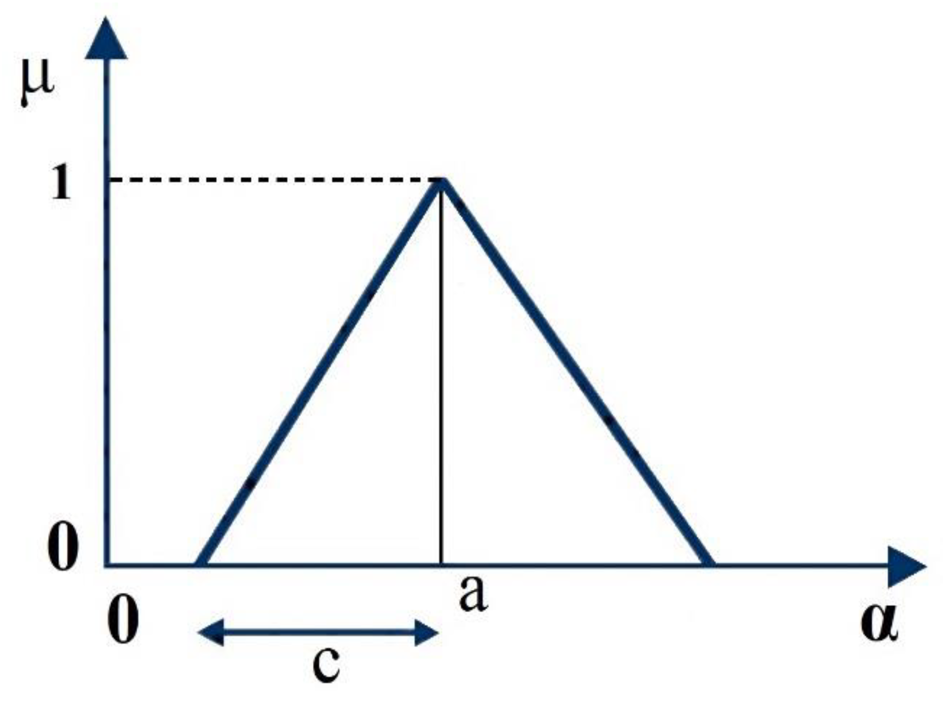
- The model is as follows:where is the fuzzy dependent variable; j = 1, …, m; i = 1, …, n; = (ai, ci) are symmetric fuzzy triangular numbers selected as coefficients; and x is the independent variable (Figure 1). In addition, n is the number of independent variables; m is the number of data; a is the central value (where μ = 1); and c is the semi-width.
- Determination of the degree h at which the data [(x1j, x2j, …, xnj), yj] is aimed to be included in the estimated number Yj:The constraints express the concept of inclusion in case that the output data are crisp numbers. In the examined case of the widely used model of Tanaka [47], a more soft definition of the fuzzy subsethood is used compared to the Zadeh [42] definition. Hence, the inclusion of a fuzzy set A into the fuzzy set B with the associated degree is defined as follows:In our case, since the data are crisp (for each individual data), the set A is only a crisp value (a point of data which must be included in the produced fuzzy band) and the fuzzy set B is a fuzzy triangular number. Hence, Equation (11) is equivalent to:It must be clarified that the above equations hold for a specified h-cut and not for every α-cut. Normally, the 0-strongcut is used since greater levels of h lead to a greater uncertainty.
- Determination of the minimization function (objective function) J. In the conventional fuzzy linear regression model, the objective function, J, is the sum of the produced fuzzy semi-widths for the data:where c0 is the semi-width of the constant term; and ci semi-width of the other fuzzy coefficients.Since fuzzy symmetric triangular numbers are selected as fuzzy coefficients, it can be proved that the objective function is the sum of the semi-widths of the produced fuzzy band regarding the available data:where the right and the left-hand side of the 0-strongcut, respectively.
- The problem results in the following linear programming problem:where ci ≥ 0, for i = 0, 1, …, n.In addition, many times, when data are classic numbers, we can easily approximate non-linear cases with the fuzzy linear regression model with the help of auxiliary variables. In this case, the total uncertainty (cumulative width) indicates incomplete complexity, whereas non-physical behavior is an indicator of overtraining [77], due to adoption of excessive complexity in non-linear models.
4.3. Implementation
For the modulation of the auxiliary variables X1, X2, X3, X4 and X5, several parameters had to be calculated. The sedimentation rate in the unit stream power equation of Yang Equation (4) was determined by means of Zanke’s [78] formula:
where ν is the water kinematic viscosity (m2/s); D* is the Bonnefille number; and dch the characteristic grain diameter (m). The Bonnefille number, D*, is given by:
In the above relation, is the density of sediment (kg/m3) and is the density of water (kg/m3).
The kinematic viscosity, ν, of water is given by the equation:
where T (°C) is the temperature of the water.
The shear velocity, , was determined by means of the following formula:
where g is the gravitational acceleration (m/s2); h (m) is the flow depth; and S is the energy slope (m/m). In Equation (20), the hydraulic radius is replaced approximately by the flow depth. In the case of uniform flow, the energy slope equals the bed slope.
When the auxiliary variables X1, X2, X3, X4 and X5 Equation (21) are introduced into the fuzzified version of the Yang’s equation Equation (4), then Equation (22) results in:
The dependent variable is the logarithm of the concentration of the total load, CF, which is produced as fuzzy symmetric triangular number, as well. By introducing the above auxiliary variables X1 to X5 for numeric data, the problem of non-linear fuzzy regression is reduced to a linear fuzzy regression problem. In the fuzzy linear regression model, the coefficients of the independent variables are fuzzy numbers that were determined using the Matlab program.
Furthermore, a simplified version of the Yang’s Equation (4), which contains only the exerted unit stream power minus the critical unit stream power, is investigated:
A criterion for the successfulness of this simplification will be the produced uncertainty. More analytically, if the uncertainty is increased significantly, this will indicate an irrational simplification (undertraining behavior).
5. Results
The comprehensive results of the calculation of the remainder parameters, as well as the results of both the classic multiple regression and fuzzy regression analyses, are presented in the following sections.
5.1. Determination of Yang’s Formula Independent Variables
As demonstrated in Section 4.3, in an effort to determine the dimensionless independent variables of Equation (4), a set of supplementary hydraulic parameters, in addition to those displayed in Table 1, had to be calculated. Hence, the following parameters were computed, on the basis of available data: water kinematic viscosity, fall velocity, shear velocity, and the dimensionless critical velocity, Vcr/ω.
Fall velocity was deemed to be the most decisive parameter in Yang’s formula, as it is the only parameter that appears in all independent variables. For this reason, a special attention was given to fall velocity, which was calculated by two widely used formulas for settling particles, those of Zanke [78] and Rubey [2]. Following the computation of kinematic viscosity and shear velocity, the dimensionless critical velocity, Vcr/ω, was calculated, for each set of data, by means of Equations (5) and (6). The ranges of values for all calculated parameters and variables, for each dataset, are provided in Table 2.
In Table 2, X1, X2, X3, X4, X5 are the dimensionless variables log(ω·d50/ν), log(/ω), log(VS/ω−VcrS/ω), log(ω·d50/ν)·log(VS/ω−VcrS/ω), log(/ω)·log(VS/ω−VcrS/ω), respectively, Ct is the total measured sediment concentration obtained from the experimental data, and CF is the total calculated sediment concentration, as obtained from the unit stream power formula, using Yang’s coefficients and by replacing the independent variables with the calculated values of X1, X2, X3, X4, X5.
As mentioned above, the calculations were carried out two times, one by using the fall velocity obtained by the formula of Zanke [78], and one with the fall velocity from the formula of Rubey [2]. By means of comparison between the 432 values of logCt and logCF, Nash-Sutcliffe Efficiencies (NSEs) of 0.79 and 0.72 were achieved with Zanke’s and Rubey’s formulas, respectively. Hence, in Table 2, only the results obtained by the use of Zanke’s formula, for fall velocity, are presented.
As a first comment, and by observing both the range values of logCt and logCF, and the NSE value of 0.79, it can be said that the approximation between the measured and calculated results, as well as the quality of data is deemed satisfactory.
5.2. Multiple Regression Analyses
5.2.1. Multiple Regression Analysis for the Reconstruction of the Unit Stream Power Formula
As a natural sequence, and to further test the successfulness of the results, the unit stream power formula Equation (4) was rebuilt. Basically, knowing both the dependent and independent variables, the coefficients of the equation were recalculated.
In the case that the conventional least square-based regression is used, the following relation is achieved:
The coefficient of determination, R2, is equal to:
where are the measured jth value of the concentration, the calculated based on Equation (24) (crisp regression) and the mean value, respectively.
5.2.2. Fuzzy Regression Analysis
In the case that the aforementioned fuzzy regression is used, the following equation is produced:
The first term in the parentheses expresses the central value and the second term the semi-width of the produced fuzzy coefficient.
The total amount of uncertainty, namely the sum of the semi-widths regarding the available data, is:
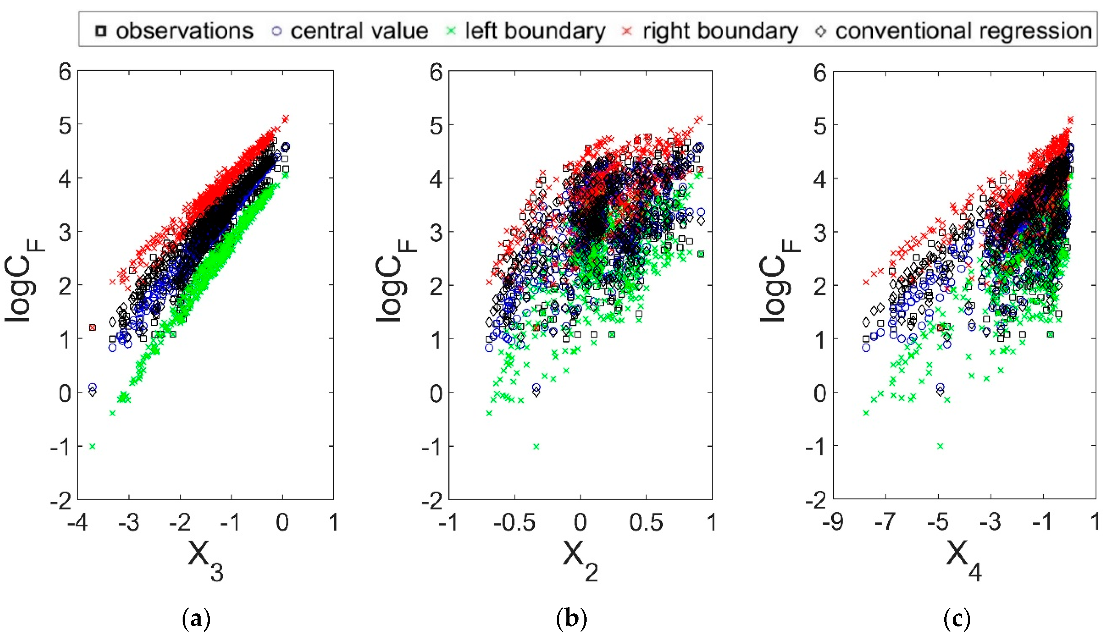
The projection of the produced logarithmic concentration Equation (26), with respect to several input variables, is presented in Figure 2.
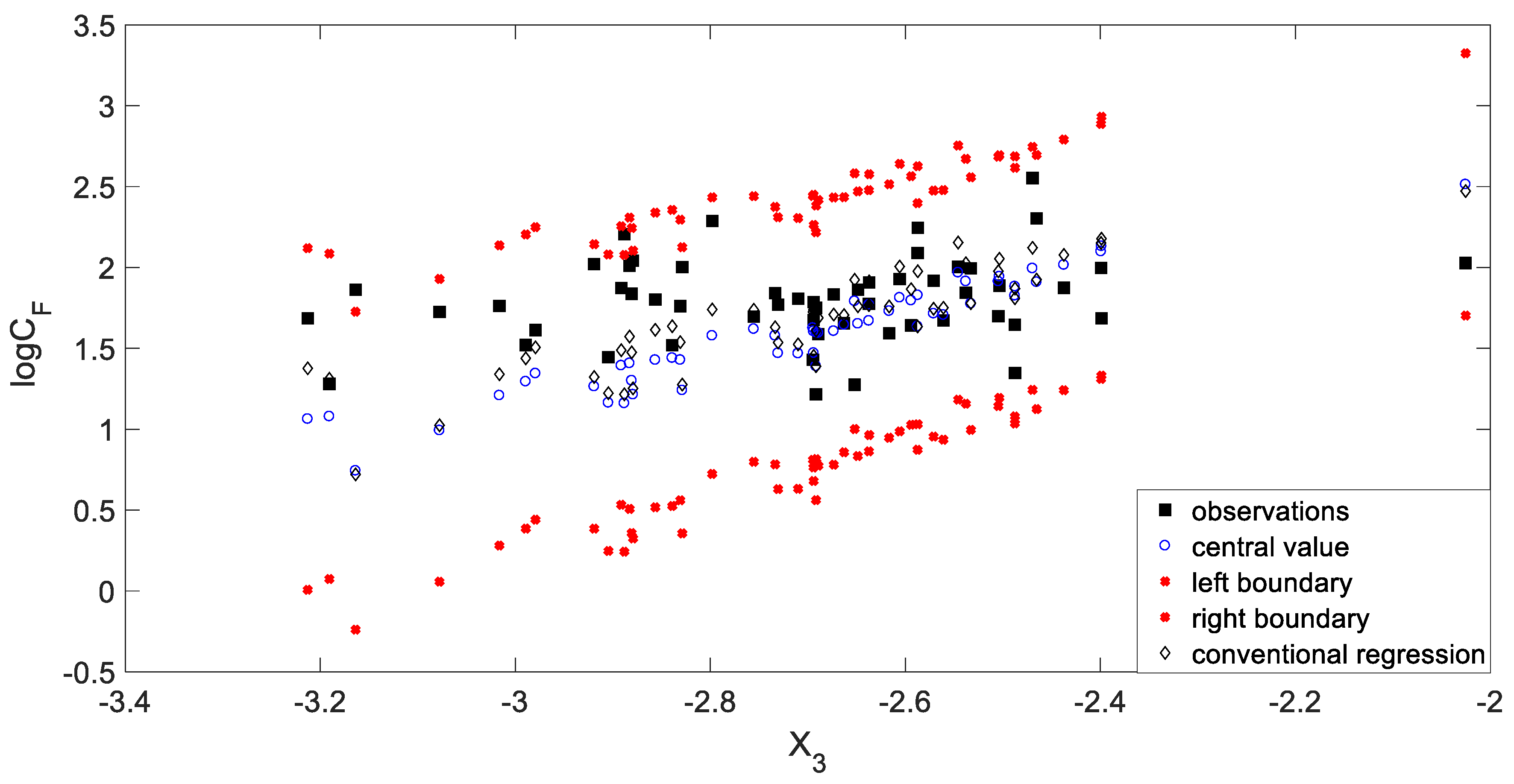
As can be seen, all the available data are included within the produced fuzzy band. Furthermore, the use of only one input variable—in this case, variable X3—is separately investigated (Figure 3). In case that the crisp linear regression is used with the X3 as the only independent variable, the results are similar, and the squared correlation coefficient, r2, is equal to 0.801. Hence, the linear dependence can be suggested. In this case, Equation (26) becomes:
and the corresponding objective function obtains the following value:
Based on the value of the objective function, J, it is obvious that this simplification (i.e., considering X3 as the only independent variable) increases the uncertainty. However, the usefulness is that the emphasis is put on the subtraction of the critical unit stream power from the exerted unit stream power, as a main independent variable. Going in the opposite direction, if only the variable X3 is removed, then the uncertainty of the produced fuzzy band is greater than the above value (J = 396.75).
An interesting perspective is that by adopting a polynomial form, in the above simplification, a small reduction of the uncertainty is achieved and hence, Equation (28) cannot be further improved. Indeed, a small reduction of the fuzzy band is achieved, if the fourth-degree polynomial regression is used.
In Figure 3, the observations against the results of the conventional linear regression, as well as the results of fuzzy linear and polynomial regressions, by using only X3 as input variable, are depicted. As it can be observed from the figure, the data of the fuzzy fourth-degree polynomial regression and the data of the fuzzy linear regression almost overlap for the most part. However, the fourth-degree polynomial regression presents an “irrational behavior” in the area of low X3 values, from a physical meaning point of view. To better explain this, as the difference “exerted unit stream power minus critical unit stream power” (here, represented by X3) grows larger, a higher sediment transport, and therefore a higher sediment concentration is expected. Simply put, logCF and X3 are similar amounts and the increase of one by the decrease of the other is not justified. The negligible reduction of the uncertainty, as well as the “irrational behavior” of the fuzzy fourth-degree polynomial regression, indicates the improperness of the polynomial models for these data. From the above it is concluded that the auxiliary variable X3 is the most significant parameter parameter. The use of high polynomial extension to Equation (28) did not improve the results. Equation (26) results in significantly less uncertainty and should be preferred.
However, a fuzzy band with high spread will include all the data, but this will be a non-useful approach. Therefore, another suitability measure, JJ, is proposed, which is equal to the mean ratio of the total spread to the central value (μ = 1, with the index j), , and when it is applied for Equation (26), it leads to the following result [37]:
where N is the number of data; in brief, the measure JJ expresses the mean uncertainty of the produced fuzzy band as a percentage of the central value. It is desirable to get low values for JJ [37]. At this point, it must be clarified that from a sediment transport point of view, the results can be characterized as sufficiently good. It should be noted that the measure JJ takes a better value compared with the corresponding JJ measure achieved by Kaffas et al. [79]. However, that study was based only on the experimental data of Guy et al. [65].
5.2.3. Validation
While the unit stream power formula was built upon only laboratory data, as stated in [80], Yang primarily built his dimensionless unit stream power equation to be used by engineers for the estimation of the total sediment concentration in both laboratory flumes and natural rivers. To make sure of the applicability of his unit stream power formula in natural streams, Yang validated it with total sediment concentrations and total suspended sediment loads from several natural rivers and streams [81,82,83,84,85]. The results revealed that Equation (4) is fairly accurate in predicting total sediment load or total bed-material load in the sand size range in natural rivers, as it is for laboratory flumes [55,80].
To test the applicability of the crisp and fuzzy regression formulas, presented in this study, data from three different sandy-bed rivers in Wisconsin, USA, taken from a US Geological Survey [86], were used. More specifically, total sediment concentration (bed load and suspended load) measurements, from Wisconsin River at Muscoda, Black River near Galesville, Chippewa River at Durand and Chippewa River near Pepin, were used for the validation of Equations (24) and (26). The median particle diameters (d50) were obtained from granulometric curves, which were constructed upon sieve analysis data, and are in a range between 0.38 mm and 0.88 mm. Along with the sediment data, basic hydraulic parameters, such as flow velocity, flow depth, energy slope and water temperature were available in the same survey. These data were used for the computation of the independent variables in Equations (24) and (26). The independent variables in any of the Equations (4), (24) or (26) represent the geometric and flow characteristics of the stream that they are applied for. A total of 55 sets of data were used for the validation of Equations (24) and (26).
Several well-known metrics, like the Root Mean Square Error (RMSE), the Mean Absolute Error (MAE), the Mean Bias Error (MBE), the Index of Agreement (d) and the NSE, were used to test the validity of the crisp multiple regression Equation (24). Though the comparison between observations and computations resulted in low statistical errors (RMSE = 0, MAE = 0.3, MBE = −0.124), and a fair Index of Agreement (d = 0.483), a negative Nash-Sutcliffe Efficiency (NSE = −1.207) (see in Appendix A) indicates that Equation (24) cannot be applied for the selected data sets. However, this was not received entirely as a surprise. Despite the validated suitability of Yang’s formula for both laboratory flumes and natural rivers in the sand range [55,80], Yang and Stall, in their report “Unit stream power for sediment transport in natural rivers” [80], stress also the constraints of the unit stream power theory for natural rivers. According to them, these constraints can be reduced to particle size, temperature and water depth. Adding to these the stream sediment transport uncertainties, mentioned in Section 3, it is realized that the successfulness of Equation (24)—which is the crisp regression—is not guaranteed for natural streams.
This deficiency of the crisp regression is overcome by the multiple fuzzy regression Equation (26), which contains 96.36% of the observed data in the fuzzy band. This can be clearly seen in Figure 4; 53 out of 55 observations are included in the produced fuzzy band of Equation (26).
In order to check the performance of the proposed fuzzy curve upon the observations, the following validation measures are proposed:
This validation measure expresses the divergence of the produced fuzzy band to include all data. In other words, the squared penalty term, E1, is activated if, and only if, the observed data are not included within the produced fuzzy band. This measure was initially proposed by Ishibuchi et al. [87] as a cost function to be minimized in the learning process, regarding a neural network with interval weights.
The second validation measure is to examine the number of points (observed data) which are outside the produced fuzzy band:
Obviously, the application of the above validation measures on the training data (laboratory data) leads to the identical values E1 = E2 = 0. By applying the validation measures to the data for natural streams, the following values are achieved: E1 = 0.1868, E2 = 2. This means that only two points do not belong to the fuzzy band (E2 = 2), but these points are not far from the produced fuzzy band, as suggested by the low value of the E1 measure.
Ultimately, the success of the crisp regression Equation (24) is not guaranteed when applied for a dataset different than the one it was created from (in this case a dataset from natural rivers). Indeed, there is a large dispersion of the measurement data from the crisp curve Equation (24) and hence, the Nash-Sutcliffe Efficiency obtains a negative value (Figure 4). Contrarily, by applying the fuzzy curve of Equation (26) for a dataset different than that it was created from, it is concluded that rather all the data is included within the produced fuzzy band with a small divergence (Figure 4). Therefore, the fuzzy curve can be used in order to achieve a fuzzy estimation of the logarithmized total sediment concentration.
6. Conclusions
The objective of this research is to transform the arithmetic coefficients of the total sediment transport rate formula of Yang, into fuzzy numbers, and thus create a fuzzy relationship that will provide a fuzzy band of in-stream sediment concentration. A very large set of experimental data, in flumes, was used for the fuzzy regression analysis. The reason for selecting the fuzzy regression is that it provides a fuzzy band not only for the coefficients of the independent variables, but for the final result, as well, which is the total sediment concentration. This means that the resulting sediment concentration is not a crisp value, but a range of values, which stretch to a value equal to the semi-width on both sides of the central value. It is proved well, by the results, that this range of values deals efficiently with the uncertainties and the ambiguous nature of sediment transport processes. Apart from the measurement errors, the computational part, and specifically the physical simplifications, i.e., one-dimensional, uniform and steady flow, grain size distribution, etc., increase the uncertainty. An interesting perspective is that even if the validation data are observations from natural rivers, where significant uncertainty and simplifications take place, these are successfully captured by the proposed fuzzy band. The minimum advantage of the fuzzy band produced is that all the data must be included. However, a main criterion is the produced width of the fuzzy band. Based on this criterion, the authors concluded that the simplification of using only one variable should be avoided, and furthermore that a determinant variable is the subtraction of the critical unit stream power from the exerted unit stream power (X3). Nevertheless, a simplification based on the X3 (i.e., only the variable X3 is taken into account) leads to a fuzzy linear curve that can be used to interpret the phenomenon. The produced fuzzy band compared with the central values indicates the good performance of the proposed fuzzy curve. In terms of elaboration of the original data utilized by Yang for the establishment of the unit stream power theory, this research goes the closest possible to what could be called “fuzzy twin” of Yang’s stream sediment transport formula.
Author Contributions
Conceptualization, M.S. (Mike Spiliotis); Methodology, M.S. (Mike Spiliotis), K.K. and V.H.; Validation, M.S. (Mike Spiliotis), K.K. and M.S. (Matthaios Saridakis); Investigation, K.K.; Data curation, K.K.; Writing—original draft preparation, K.K. and M.S. (Mike Spiliotis); Writing—review and editing, V.H., K.K., M.S. (Mike Spiliotis) and M.R.; Visualization, M.S. (Mike Spiliotis), M.S. (Matthaios Saridakis) and K.K.; Supervision, V.H. and M.S. (Mike Spiliotis). All authors have read and agreed to the published version of the manuscript.
Funding
K.K. and M.R. were supported by the project Sediplan–r (FESR1002) and financed by the European Regional Development Fund (ERDF) Investment for Growth and Jobs Programme 2014–2020.
Acknowledgments
The authors would like to express their thankfulness to the reviewers for their comments and suggestions, which helped to improve the quality of this study.
Conflicts of Interest
The authors declare no conflict of interest.
Appendix A
The Nash-Sutcliffe Efficiency (NSE), proposed by Nash and Sutcliffe in 1970, is defined as one minus the sum of the squared differences between the observed and predicted data normalized by the variance of the observed values [88]:
where are the observed values; the predicted values; the mean observed value; and j = 1, …, m.
The use of NSE is not restricted solely in regression models, but extends for any application of hydrological modeling and, therefore, in its general use, it takes values between and 1, i.e., . An efficiency lower than zero indicates that the mean value of the observed time series would have been a better predictor than the model [89]. In such cases, the model should be rejected.
At this point, the relation between the coefficient of determination, R2, and the Nash-Sutcliffe Efficiency, NSE, should be clarified. In case of a multiple regression, R2 and NSE are simply identical. However, the coefficient of determination has a value bounded between 0 and 1 [90], that is [82].
An interesting perspective is the comparison of the correlation coefficient, r, with the Nash-Sutcliffe Efficiency. In case of a conventional linear regression model with only one independent variable, the squared value of the correlation coefficient, r2, is equal to . The correlation coefficient, r, indicates the strength and the direction of a linear relationship with respect to the data, whilst it cannot imply causation.
In the present model and with regard to the training set, namely the laboratory data, in the case of the crisp multiple regression, the NSE is identical to the R2, and obviously non-negative, i.e., . However, when the crisp multiple regression equation is used upon the other validation measurements, from natural streams, then it takes negative values, i.e., .
Finally, if only one independent variable is used (in this case, X3), again for the training data, then the NSE is identical to the R2 and with the squared value of the correlation coefficient, r, .
References
- Gilbert, G.K.; Murphy, E.C. The Transportation of Debris by Running Water; US Geological Survey Professional Paper 86; US Government Printing Office: Washington, DC, USA, 1914.
- Rubey, W.W. Settling Velocities of Gravel, Sand and Silt Particles. Am. J. Sci. 1933, 148, 325–338. [Google Scholar] [CrossRef]
- Anderson, A.G.; Johnson, J.W. A Distinction Between Bed Load and Suspended Load in Natural Streams. Eos Trans. Am. Geophys. Union 1940, 21, 628–633. [Google Scholar]
- McCully, P. Silenced Rivers: The Ecology and Politics of Large Dams; Zed Books: London, UK, 1996. [Google Scholar]
- Kaffas, K.; Hrissanthou, V.; Sevastas, S. Modeling Hydromorphological Processes in a Mountainous Basin Using a Composite Mathematical Model and ArcSWAT. Catena 2018, 162, 108–129. [Google Scholar] [CrossRef]
- Kaffas, K. Development of Mathematical Model for Calculating Continuous Hydrographs and Sediment Graphs in a Basin Due to Rainfall. Ph.D. Thesis, Democritus University of Thrace, Xanthi, Greece, 28 June 2017. [Google Scholar]
- Graf, W.; Leitner, P.; Hanetseder, I.; Ittner, L.D.; Dossi, F.; Hauer, C. Ecological degradation of a meandering river by local channelization effects: A case study in an Austrian lowland river. Hydrobiologia 2016, 772, 145–160. [Google Scholar] [CrossRef]
- Spalevic, V.; Lakicevic, M.; Radanovic, D.; Billi, P.; Barovic, G.; Vujacic, D.; Sestras, P.; Darvishan, A.K. Ecological-Economic (Eco-Eco) Modelling in the River Basins of Mountainous Regions: Impact of Land Cover Changes on Sediment Yield in the Velicka Rijeka, Montenegro. Not. Bot. Horti Agrobot. Cluj-Napoca 2017, 45, 602–610. [Google Scholar] [CrossRef] [Green Version]
- Samaras, A.G.; Koutitas, C.G. Modeling the impact of climate change on sediment transport and morphology in coupled watershed–coast systems: A case study using an integrated approach. Int. J. Sed. Res. 2014, 29, 304–315. [Google Scholar] [CrossRef]
- Kondolf, G.M. PROFILE: Hungry water: Effects of dams and gravel mining on river channels. Environ. Manag. 1997, 21, 533–551. [Google Scholar] [CrossRef]
- Pisaturo, G.R.; Righetti, M. Sediment flushing from reservoir and ecological impacts. EPiC Ser. Eng. 2018, 3, 1692–1697. [Google Scholar]
- Yagci, O.; Celik, M.F.; Kitsikoudis, V.; Kirca, V.S.O.; Hodoglu, C.; Valyrakis, M.; Duran, Z.; Kaya, S. Scour patterns around isolated vegetation elements. Adv. Water Res. 2016, 97, 251–265. [Google Scholar] [CrossRef] [Green Version]
- Summerfield, M.A.; Hulton, N.J. Natural controls of fluvial denudation rates in major world drainage basins. J. Geophys. Res. 1994, 99, 13871–13883. [Google Scholar] [CrossRef]
- Galy, A.; France-Lanord, C. Higher erosion rates in the Himalaya: Geochemical constraints on riverine fluxes. Geology 2001, 29, 23–26. [Google Scholar] [CrossRef]
- Lavé, J.; Avouac, J.P. Fluvial incision and tectonic uplift across the Himalayas of central Nepal. J. Geophys. Res. 2001, 106, 26561–26591. [Google Scholar] [CrossRef]
- Turowski, J.M.; Rickenmann, D.; Dadson, S.J. The partitioning of the total sediment load of a river into suspended load and bedload: A review of empirical data. Sedimentology 2010, 57, 1126–1146. [Google Scholar] [CrossRef]
- Meyer–Peter, E.; Müller, R. Formulas for bed-load transport. In Proceedings of the International Association for Hydraulic Research, 2nd Meeting, Stockholm, Sweden, 7 June 1948. [Google Scholar]
- Camenen, B.; Larson, M.A. General formula for non-cohesive bed load sediment transport. Estuar. Coast. Shelf Sci. 2005, 63, 249–260. [Google Scholar] [CrossRef]
- Lane, E.W.; Kalinske, A.A. Engineering calculations of suspended sediment. Eos Trans. Am. Geophys. Union 1941, 22, 603–607. [Google Scholar] [CrossRef]
- van Rijn, L.C. Sediment transport, part II: Suspended load transport. J. Hydraul. Eng. 1984, 110, 1613–1641. [Google Scholar] [CrossRef]
- Ackers, P.; White, W.R. Sediment transport: New approach and analysis. ASCE J. Hydraul. Div. 1973, 99, 204–254. [Google Scholar]
- Yang, C.T. Incipient motion and sediment transport. ASCE J. Hydraul. Div. 1973, 99, 1679–1704. [Google Scholar]
- Schriften, D.V.W.K. Feststofftransport in Fließgewässern-Berechnungsverfahren für die Ingenieurpraxis; Heft 87; Verlag Paul Parey: Hamburg/Berlin, Germany, 1988. [Google Scholar]
- Einstein, H.A. The Bed-Load Function for Sediment Transportation in Open Channel Flows; No. 1488-2016-124615; US Department of Agriculture Technical Bulletin: Washington, DC, USA, 1950.
- Toffaleti, F.B. Definitive computation of sand discharge in rivers. ASCE J. Hydraul. Div. 1969, 95, 225–248. [Google Scholar]
- Karim, M.F.; Holly, F.M.; Kennedy, J.F. Bed Armoring Procedures in IALLUVIAL and Application to the Missouri River; No. 269; Iowa Institute of Hydraulic Research, University of Iowa: Iowa City, IA, USA, 1983. [Google Scholar]
- Yang, C.T. Unit stream power and sediment transport. ASCE J. Hydraul. Div. 1972, 98, 1805–1826. [Google Scholar]
- Engelund, F.; Hansen, E. A Monograph on Sediment Transport in Alluvial Streams; Teknisk Forlag: Copenhagen, Denmark, 1967. [Google Scholar]
- Zanke, U. Grundlagen der Sedimentbewegung; Springer: Berlin/Heidelberg, Germany, 1982. [Google Scholar]
- van Rijn, L.C. Closure to “Sediment transport, part I: Bed load transport”. ASCE J. Hydraul. Eng. 1984, 110, 1431–1456. [Google Scholar] [CrossRef] [Green Version]
- Yang, C.T. Sediment Transport: Theory and Practice, reprint ed.; Krieger: Malabar, FL, USA, 2003. [Google Scholar]
- Yang, C.T. Unit stream power equation for gravel. ASCE J. Hydraul. Eng. 1984, 110, 1783–1797. [Google Scholar] [CrossRef]
- Aqil, M.; Kita, I.; Yano, A.; Nishiyama, S. Analysis and prediction of flow from local source in a river basin using a neuro-fuzzy modeling tool. J. Env. Manag. 2007, 85, 215–223. [Google Scholar] [CrossRef] [PubMed]
- Zhu, S.; Heddam, S.; Nyarko, E.K.; Hadzima-Nyarko, M.; Piccolroaz, S.; Wu, S. Modeling daily water temperature for rivers: comparison between adaptive neuro-fuzzy inference systems and artificial neural networks models. Environ. Sci. Pollut. Res. 2019, 26, 402–420. [Google Scholar] [CrossRef] [PubMed]
- Tayfur, G.; Ozdemir, S.; Singh, V.P. Fuzzy logic algorithm for runoff-induced sediment transport from bare soil surfaces. Adv. Water Res. 2003, 26, 1249–1256. [Google Scholar] [CrossRef] [Green Version]
- Chachi, J.; Taheri, S.M.; Pazhand, H.R. Suspended load estimation using L1—Fuzzy regression, L2—Fuzzy regression and MARS—fuzzy regression models. Hydrol. Sci. J. 2016, 61, 1489–1502. [Google Scholar] [CrossRef]
- Spiliotis, M.; Kitsikoudis, V.; Kirca, V.S.O.; Hrissanthou, V. Fuzzy threshold for the initiation of sediment motion. App. Soft Comp. 2018, 72, 312–320. [Google Scholar] [CrossRef]
- Zanke, U.C.E. On the influence of turbulence on the initiation of sediment motion. Int. J. Sed. Res. 2003, 18, 17–31. [Google Scholar]
- Spiliotis, M.; Kitsikoudis, V.; Hrissanthou, V. Assessment of bedload transport in gravel-bed rivers with a new fuzzy adaptive regression. Eur. Water 2017, 57, 237–244. [Google Scholar]
- Kitsikoudis, V.; Spiliotis, M.; Hrissanthou, V. Fuzzy regression analysis for sediment incipient motion under turbulent flow conditions. Environ. Proc. 2016, 3, 663–679. [Google Scholar] [CrossRef]
- Özger, M.; Kabataş, M.B. Sediment load prediction by combined fuzzy logic—Wavelet method. J. Hydroinf. 2015, 17, 930–942. [Google Scholar] [CrossRef]
- Kişi, Ö. Evolutionary fuzzy models for river suspended sediment concentration estimation. J. Hydrol. 2009, 372, 68–79. [Google Scholar] [CrossRef]
- Kişi, Ö.; Karahan, M.E.; Şen, Z. River suspended sediment modelling using a fuzzy logic approach. Hydrol. Proc. Int. J. 2006, 20, 4351–4362. [Google Scholar] [CrossRef]
- Lohani, A.K.; Goel, N.K.; Bhatia, K.S. Deriving stage—Discharge—Sediment concentration relationships using fuzzy logic. Hydrol. Sci. J. 2007, 52, 793–807. [Google Scholar] [CrossRef]
- Zadeh, L.A. Fuzzy sets. Inf. Control 1965, 8, 338–353. [Google Scholar] [CrossRef] [Green Version]
- Firat, M.; Güngör, M. Monthly total sediment forecasting using adaptive neuro-fuzzy inference system. Stoch. Environ. Res. Risk Assess. 2010, 24, 259–270. [Google Scholar] [CrossRef]
- Tanaka, H. Fuzzy data analysis by possibilistic linear models. Fuzzy Sets Syst. 1987, 24, 363–375. [Google Scholar] [CrossRef]
- Kaffas, K.; Hrissanthou, V. Estimate of continuous sediment graphs in a basin, using a composite mathematical model. Environ. Proc. 2015, 2, 361–378. [Google Scholar] [CrossRef] [Green Version]
- Kaffas, K.; Hrissanthou, V. Computation of hourly sediment discharges and annual sediment yields by means of two soil erosion models in a mountainous basin. Int. J. River Basin Manag. 2019, 17, 63–77. [Google Scholar] [CrossRef]
- Nakato, T. Tests of selected sediment—Transport formulas. J. Hydraul. Eng. 1990, 116, 362–379. [Google Scholar] [CrossRef]
- Baosheng, W.U.; van Maren, D.S.; Lingyun, L.I. Predictability of sediment transport in the Yellow River using selected transport formulas. Int. J. Sed. Res. 2008, 23, 283–298. [Google Scholar]
- Moore, I.D.; Burch, G.J. Sediment transport capacity of sheet and rill flow: Application of unit stream power theory. Water Res. Res. 1986, 22, 1350–1360. [Google Scholar] [CrossRef]
- Hui-Ming, S.; Yang, C.T. Estimating overland flow erosion capacity using unit stream power. Int. J. Sed. Res. 2009, 24, 46–62. [Google Scholar]
- Hrissanthou, V.; Hartmann, S. Measurements of critical shear stress in sewers. Water Res. 1998, 32, 2035–2040. [Google Scholar] [CrossRef]
- Yang, C.T. Unit stream power equations for total load. J. Hydrol. 1979, 40, 123–138. [Google Scholar] [CrossRef]
- Salas, J.D.; Shin, H.S. Uncertainty analysis of reservoir sedimentation. J. Hydraul. Eng. 1999, 125, 339–350. [Google Scholar] [CrossRef]
- Kleinhans, M.G. Flow discharge and sediment transport models for estimating a minimum timescale of hydrological activity and channel and delta formation on Mars. J. Geophys. Res. Planets 2005, 110. [Google Scholar] [CrossRef] [Green Version]
- Fischer, S.; Pietroń, J.; Bring, A.; Thorslund, J.; Jarsjö, J. Present to future sediment transport of the Brahmaputra River: Reducing uncertainty in predictions and management. Reg. Environ. Chang. 2017, 17, 515–526. [Google Scholar] [CrossRef] [Green Version]
- Beckers, F.; Noack, M.; Wieprecht, S. Uncertainty analysis of a 2D sediment transport model: An example of the Lower River Salzach. J. Soils Sediments 2017, 18, 3133–3144. [Google Scholar] [CrossRef]
- Azamathulla, H.M.; Ghani, A.A.; Fei, S.Y. ANFIS-based approach for predicting sediment transport in clean sewer. Appl. Soft Comp. 2012, 12, 1227–1230. [Google Scholar] [CrossRef] [Green Version]
- Nomicos, G.N. Effects of Sediment Load on the Velocity Field and Friction Factor of Turbulent Flow in an Open Channel. Ph.D. Thesis, California Institute of Technology, Pasadena, CA, USA, 1956. [Google Scholar]
- Vanoni, V.A.; Brooks, N.H. Laboratory Studies of the Roughness and Suspended Load of Alluvial Streams; Report No. E-68; Sedimentation Laboratory, California Institute of Technology: Pasadena, CA, USA, 1957. [Google Scholar]
- Kennedy, J.F. Stationary Waves and Antidunes in Alluvial Channels; Report No. KH-R-2; W.M. Keck Laboratory of Hydraulics and Water Resources, California Institute of Technology: Pasadena, CA, USA, 1961. [Google Scholar]
- Stein, R.A. Laboratory studies of total load and apparent bed-load. J. Geophys. Res. 1965, 70, 1831–1842. [Google Scholar] [CrossRef]
- Guy, H.P.; Simons, D.B.; Richardson, E.V. Summary of Alluvial Channel Data from Flume Experiment, 1956–1961; US Geological Survey Professional Paper: Washington, DC, USA, 1966.
- Williams, G.P. Flume Experiments on the Transport of a Coarse Sand; US Geological Survey Professional Paper: Reston, VA, USA, 1967.
- Schneider, V.R. Personal Communication of Yang. Data Collected from an 8-Foot Wide Flume at Colorado State University; Colorado State University: Fort Collins, CO, USA, 1971. [Google Scholar]
- Simons, D.B.; Richardson, E.V.; Albertson, M.L. Flume studies using medium sand (0.45 mm); US Geological Survey Water-Supply Paper: Washington, DC, USA, 1961.
- Inter-Agency Committee on Water Resources, Subcommittee on Sedimentation. Some Fundamentals of Particle Size Analysis; St. Anthony Falls Hydraulic Laboratory: Minneapolis, MN, USA, 1957. [Google Scholar]
- Tsakiris, G.; Spiliotis, M. Uncertainty in the analysis of urban water supply and distribution systems. J. Hydroinf. 2017, 19, 823–837. [Google Scholar] [CrossRef] [Green Version]
- Papadopoulos, C.; Spiliotis, M.; Angelidis, P.; Papadopoulos, B. A hybrid fuzzy frequency factor based methodology for analyzing the hydrological drought. J. Desal. Water Treat. 2019, 167, 385–397. [Google Scholar] [CrossRef]
- Klir, G.; Yuan, B. Fuzzy Sets and Fuzzy Logic: Theory and Applications; Prentice Hall: Upper Saddle River, NJ, USA, 1995; p. 574. [Google Scholar]
- Buckley, J.; Eslami, E. An Introduction to Fuzzy Logic and Fuzzy Sets; Springer: Berlin, Germany, 2002; p. 285. [Google Scholar]
- Hanss, M. Applied Fuzzy Arithmetic, an Introduction with Engineering Applications; Springer: Berlin, Germany, 2005; p. 256. [Google Scholar]
- Spiliotis, M.; Angelidis, P.; Papadopoulos, B. A hybrid probabilistic bi-sector fuzzy regression based methodology for normal distributed hydrological variable. Evol. Syst. 2019, 1–14. [Google Scholar] [CrossRef]
- Tsakiris, G.; Tigkas, D.; Spiliotis, M. Assessment of interconnection between two adjacent watersheds using deterministic and fuzzy approaches. Eur. Water 2006, 15, 15–22. [Google Scholar]
- Spiliotis, M.; Hrissanthou, V. Fuzzy and crisp regression analysis between sediment transport rates and stream discharge in the case of two basins in northeastern Greece. In Conventional and Fuzzy Regression: Theory and Engineering Applications, 1st ed.; Hrissanthou, V., Spiliotis, M., Eds.; Nova Science Publishers: New York, NY, USA, 2018; pp. 1–49. [Google Scholar]
- Zanke, U. Berechung der Sinkgeschwindigkeiten von Sedimenten; Mitt. des Franzius-Instituts für Wasserbau, Technical University of Hannover: Hannover, Germany, 1977. [Google Scholar]
- Kaffas, K.; Saridakis, M.; Tsangaratos, P.; Spiliotis, M.; Hrissanthou, V. Application of Υang formula for calculating total sediment transport rate with fuzzy regression. In Proceedings of the 14th Conference of the Hellenic Hydrotechnical Association, Volos, Greece, 16–17 March 2019. (In Greek). [Google Scholar]
- Yang, C.T.; Stall, J.B. Unit Stream Power for Sediment Transport in Natural Rivers; WRC Research Report 88; Water Resources Centre, University of Illinois: Urbana-Champaign Water Resources Center, IL, USA, 1974. [Google Scholar]
- Einstein, H.A. Bed-Load Transportation in Mountain Creek; United States Department of Agriculture, Soil Conservation Service: Washington, DC, USA, 1944.
- Colby, B.R.; Hembree, C.H. Computation of Total Sediment Discharge, Niobrara River near Cody, Nebraska; Water Supply Paper 1357; US Geological Survey: Washington, DC, USA, 1955.
- Hubbell, D.W.; Matejka, D.Q. Investigations of Sediment Transportation, Middle Loup River at Dunning, Nebraska; Water Supply Paper 1376; US Geological Survey: Washington, DC, USA, 1959.
- Nordin, C.F. Aspects of Flow Resistance and Sediment Transport, Rio Grande River near Bernalillo, New Mexico; Water Supply Paper 1398-H; US Geological Survey: Washington, DC, USA, 1964.
- Jordan, P.R. Fluvial Sediment of the Mississippi River at St. Louis, Missouri; Water Supply Paper 1802; US Geological Survey: Washington, DC, USA, 1965.
- Williams, G.P.; Rosgen, D.L. Measured Total Sediment Loads (Suspended Loads and Bedloads) for 93 United States Streams; Open File Report; US Geological Survey: Reston, VA, USA, 1989.
- Ishibuchi, H.; Tanaka, H.; Okada, H. An architecture of neural networks with interval weights and its application to fuzzy regression analysis. Fuzzy Sets Syst. 1993, 57, 27–39. [Google Scholar] [CrossRef]
- Nash, J.E.; Sutcliffe, J.V. River flow forecasting through conceptual models: Part 1. A discussion of principles. J. Hydrol. 1970, 10, 282–290. [Google Scholar] [CrossRef]
- Krause, P.; Boyle, D.P.; Bäse, F. Comparison of different efficiency criteria for hydrological model assessment. Adv. Geosci. 2005, 5, 89–97. [Google Scholar] [CrossRef] [Green Version]
- Mays, L.; Tung, Y.K. Water distribution systems. In Hydrosystems Engineering and Management; McGraw-Hill: New York, NY, USA, 1992; pp. 354–386. [Google Scholar]
Figure 1.
Fuzzy symmetric triangular number.

Figure 2.
Projection of the achieved fuzzy relation regarding the log of the total sediment concentration with respect to (a) X3, (b) X2, (c) X4.
Figure 2.
Projection of the achieved fuzzy relation regarding the log of the total sediment concentration with respect to (a) X3, (b) X2, (c) X4.

Figure 3.
Fuzzy linear regression to achieve the log of the total sediment concentration with respect to X3.
Figure 3.
Fuzzy linear regression to achieve the log of the total sediment concentration with respect to X3.

Figure 4.
Multiple fuzzy regression of total sediment concentration in natural streams.


Table 1.
Experimental data for unit stream power equation.
| Particle Size, d50 (mm) | Channel Length, L (ft) | Channel Width, W (ft) | Water Depth, h (ft) | Temperature, T (°C) | Average Velocity, V (ft/s) | Water Surface Slope, S×103 | Total Sediment Concentration, Ct (ppm) | Number of Data, N |
|---|---|---|---|---|---|---|---|---|
| Nomicos’ data (1956) [61] | ||||||||
| 0.152 | 40 | 0.875 | 0.241 | 25.0–26.0 | 0.80–2.63 | 2.0–3.9 | 300–5767 | 12 |
| Vanoni and Brooks’ data (1957) [62] | ||||||||
| 0.137 | 60 | 2.79 | 0.147–0.346 | 18.9–27.4 | 0.77–2.53 | 0.7–2.8 | 37–3000 | 14 |
| Kennedy’s data (1961) [63] | ||||||||
| 0.233 | 40 | 0.875 | 0.147–0.346 | 24.5–30.1 | 1.57–3.42 | 2.6–16.0 | 730–34,700 | 14 |
| 0.549 | 40 | 0.875 | 0.074–0.346 | 24.3–27.0 | 1.65–4.65 | 5.5–27.2 | 1680–35,900 | 14 |
| 0.233 | 60 | 2.79 | 0.145–0.356 | 23.0–27.3 | 1.35–3.45 | 1.7–22.9 | 490–58,500 | 13 |
| Stein’s data (1965) [64] | ||||||||
| 0.4 | 100 | 4.0 | 0.59–1.20 | 20.0–28.9 | 1.38–5.51 | 0.61–10.79 | 93–24,249 | 42 |
| Guy et al. data (1966) [65] | ||||||||
| 0.19 | 150 | 8.0 | 0.49–1.09 | 12.3–19.7 | 1.04–4.74 | 0.43–9.50 | 29–47,300 | 29 |
| 0.27 | 150 | 8.0 | 0.45–1.13 | 10.2–18.5 | 1.24–4.93 | 0.46–10.22 | 12–35,800 | 18 |
| 0.28 | 150 | 8.0 | 0.30–1.07 | 10.2–17.6 | 1.04–4.93 | 0.45–10.07 | 12–42,400 | 33 |
| 0.48(0.45) | 150 | 8.0 | 0.19–1.00 | 9.0–20.0 | 0.75–6.18 | 0.39–10.10 | 10–15,100 | 34 |
| 1.2(0.93) | 150 | 8.0 | 0.38–1.11 | 16.7–21.7 | 1.46–6.07 | 0.37–12.80 | 15–10,200 | 32 |
| 0.32 | 60 | 2.0 | 0.54–0.74 | 7.0–34.3 | 1.24–5.73 | 0.86–16.20 | 55–49,300 | 29 |
| 0.33 (uniform) | 60 | 2.0 | 0.49–0.52 | 19.8–20.3 | 1.17–6.93 | 0.88–11.40 | 47–18,400 | 12 |
| 0.33 (graded) | 60 | 2.0 | 0.48–0.53 | 19.6–24.1 | 1.06–6.34 | 0.47–9.80 | 12–22,500 | 14 |
| 0.50(0.47) | 150 | 8.0 | 0.30–1.33 | 10.7–24.5 | 4.69–17.45 | 0.42–9.60 | 23–17,700 | 50 |
| 0.59(0.54) | 60 | 2.0 | 0.59–0.89 | 16.9–25.1 | 1.37–6.27 | 0.38–19.28 | 17–50,000 | 35 |
| Williams’ data (1967) [66] | ||||||||
| 1.35 | 52 | 1.0 | 0.094–0.517 | 11.9–30.8 | 1.27–3.49 | 1.10–22.18 | 10–9223 | 37 |
| Schneider’s data (1971) [67] | ||||||||
| 0.25 | – | 8.0 | 1.012–2.822 | 20.4–22.4 | 1.67–6.45 | 0.10–4.97 | 18–17,152 | 31 |
Table 2.
Calculated parameters and variables for unit stream power equation.
| Kinematic Viscosity × 10−6, ν (m2/s) | Fall Velocity, ω (m/s), Zanke (1977) | Shear Velocity, V*(m/s) | Dimensionless Critical Velocity, Vcr/ω | X1 | X2 | X3 | X4 | X5 | Total Measured Sediment Concentration, Ct (ppm) | logCt | Total Calculated Sediment Concentration, CF (ppm) | logCF | Number of Data, N |
|---|---|---|---|---|---|---|---|---|---|---|---|---|---|
| Nomicos’ data (1956) [61] | |||||||||||||
| 0.88 | 0.02 | 0.04–0.05 | 3.46–4.0 | 0.53–0.54 | 0.27–0.43 | −1.79–(−0.84) | −0.97–(−0.44) | −0.52–(−0.36) | 300–5767 | 2.48–3.76 | 303–7387 | 2.48–3.87 | 12 |
| Vanoni and Brooks’ data (1957) [62] | |||||||||||||
| 0.85–1.04 | 0.015–0.017 | 0.03–0.05 | 3.87–4.77 | 0.29–0.45 | 0.29–0.46 | −1.98–(−0.98) | −0.74–(−0.28) | −0.71–(−0.42) | 37–3000 | 1.57–3.48 | 132–4419 | 2.12–3.65 | 14 |
| Kennedy’s data (1961) [63] | |||||||||||||
| 0.8–0.91 | 0.04–0.04 | 0.04–0.09 | 2.56–3.26 | − | 0.01–0.36 | −1.53–(−0.43) | −1.56–(−0.44) | −0.22–(−0.01) | 730–34,700 | 2.86–4.54 | 1070–27,619 | 3.03–4.44 | 14 |
| 0.86–0.91 | 0.08–0.09 | 0.05–0.1 | 2.09–2.42 | 1.72–1.75 | −0.24–0.06 | −1.73–(−0.42) | −2.97–(−0.73) | −0.02–0.42 | 1680–35,900 | 3.23–4.56 | 1075–29,057 | 3.03–4.46 | 14 |
| 0.85–0.94 | 0.036–0.038 | 0.04–0.12 | 2.4–3.34 | 0.96–1.02 | 0.02–0.52 | −1.7–(−0.25) | −1.7–(−0.24) | −0.22–(−0.02) | 490–58,500 | 2.69–4.77 | 619–40,833 | 2.79–4.61 | 13 |
| Stein’s data (1965) [64] | |||||||||||||
| 0.83–1.01 | 0.065–0.069 | 0.04–0.14 | 2.12–2.75 | 1.41–1.52 | −0.19–0.32 | −2.66–(−0.61) | −3.85–(−0.88) | −0.25–0.51 | 93–24,249 | 1.97–4.39 | 55–15,860 | 1.74–4.2 | 42 |
| Guy et al. data (1966) [65] | |||||||||||||
| 1.02–1.23 | 0.01–0.02 | 0.04–0.14 | 2.62–4.94 | 0.09–0.55 | 0.24–0.81 | −2.0–(−0.26) | −1.1–(−0.10) | −0.9–(−0.21) | 29–47,300 | 1.46–4.68 | 122–38,227 | 2.09–4.58 | 29 |
| 1.05–1.3 | 0.02–0.04 | 0.04–0.14 | 2.67–3.82 | 0.51–0.85 | 0.1–0.79 | −2.38–(−0.22) | −1.79–(−0.12) | −0.66–(−0.17) | 12–35,800 | 1.08–4.55 | 50–42,848 | 1.7–4.63 | 18 |
| 1.07–1.3 | 0.1–0.04 | 0.04–0.13 | 2.65–4.22 | 0.13–0.99 | −0.06–0.83 | −2.51–(−0.24) | −2.49–(−0.14) | −0.88–0.14 | 12–42,400 | 1.08–4.63 | 43–41,340 | 1.64–4.62 | 33 |
| 1.01–1.35 | 0.01–0.08 | 0.03–0.11 | 2.26–4.66 | 0.19–1.56 | −0.34–0.92 | −3.72–(−0.37) | −4.92–(−0.22) | −1.04–1.25 | 10–15,100 | 1.0–4.18 | 1–28,845 | 0.15–4.46 | 34 |
| 0.97–1.1 | 0.05–0.12 | 0.03–0.13 | 2.05–2.54 | 1.5–2.16 | −0.59–0.37 | −3.13–(−0.63) | −6.7–(−1.19) | −0.45–1.84 | 15–10,200 | 1.18–4.01 | 28–15,613 | 1.45–4.19 | 32 |
| 0.74–1.43 | 0.02–0.06 | 0.04–0.18 | 2.29–3.86 | 0.57–1.46 | −0.13–0.73 | −2.33–(−0.17) | −3.33–(−0.15) | −0.59–0.3 | 55–49,300 | 1.74–4.69 | 105–45,297 | 2.02–4.66 | 29 |
| 1.0–1.02 | 0.02–0.05 | 0.04–0.13 | 2.34–4.24 | 0.71–1.27 | 0.05–0.5 | −2.05–(−0.27) | −2.11–(−0.3) | −0.63–(−0.09) | 47–18,400 | 1.67–4.27 | 176–37,507 | 2.25–4.57 | 12 |
| 0.92–1.02 | 0.01–0.05 | 0.03–0.12 | 2.82–5.95 | 0.09–1.19 | −0.2–0.91 | −2.46–0.07 | −2.94–0.03 | −0.82–0.49 | 12–22,500 | 1.08–4.35 | 64–93,556 | 1.81–4.97 | 14 |
| 0.91–1.28 | 0.03–0.08 | 0.03–0.11 | 2.15–3.54 | 0.82–1.74 | −0.36–0.39 | −1.99–(−0.21) | −2.77–(−0.3) | −0.39–0.647 | 23–17,700 | 1.362–4.25 | 314–48,987 | 2.5–4.69 | 50 |
| 0.9–1.09 | 0.06–0.09 | 0.03–0.2 | 2.05–3.17 | 1.35–1.79 | −0.45–0.44 | −3.02–(−0.37) | −4.66–(−0.55) | −0.23–1.37 | 17–50,000 | 1.23–4.7 | 17–26,180 | 1.24–4.42 | 35 |
| Williams’ data (1967) [66] | |||||||||||||
| 0.79–1.24 | 0.15–0.16 | 0.03–0.1 | 2.05–2.25 | 2.22–2.43 | −0.7–(−0.2) | −3.33–(−1.07) | −7.75–(−2.53) | 0.23–2.31 | 10–9223 | 1.0–3.97 | 35–8038 | 1.55–3.91 | 37 |
| Schneider’s data (1971) [67] | |||||||||||||
| – | – | – | – | – | – | – | – | – | 18–17,152 | – | – | – | 31 |
© 2020 by the authors. Licensee MDPI, Basel, Switzerland. This article is an open access article distributed under the terms and conditions of the Creative Commons Attribution (CC BY) license (http://creativecommons.org/licenses/by/4.0/).
Share and Cite
MDPI and ACS Style
Kaffas, K.; Saridakis, M.; Spiliotis, M.; Hrissanthou, V.; Righetti, M. A Fuzzy Transformation of the Classic Stream Sediment Transport Formula of Yang. Water 2020, 12, 257. https://doi.org/10.3390/w12010257
AMA Style
Kaffas K, Saridakis M, Spiliotis M, Hrissanthou V, Righetti M. A Fuzzy Transformation of the Classic Stream Sediment Transport Formula of Yang. Water. 2020; 12(1):257. https://doi.org/10.3390/w12010257
Chicago/Turabian StyleKaffas, Konstantinos, Matthaios Saridakis, Mike Spiliotis, Vlassios Hrissanthou, and Maurizio Righetti. 2020. "A Fuzzy Transformation of the Classic Stream Sediment Transport Formula of Yang" Water 12, no. 1: 257. https://doi.org/10.3390/w12010257
Note that from the first issue of 2016, this journal uses article numbers instead of page numbers. See further details here.