Discharge Coefficients for Sluice Gates Set in Weirs at Different Upstream Wall Inclinations


Fluid Dynamics Laboratory, Dipartimento di Ingegneria Civile, Università della Calabria, Via P. Bucci, Cubo 42b, 87036 Rende, Italy
*
Author to whom correspondence should be addressed.
Water 2020, 12(1), 245; https://doi.org/10.3390/w12010245
Submission received: 17 December 2019
/
Revised: 8 January 2020
/
Accepted: 13 January 2020
/
Published: 15 January 2020
(This article belongs to the Special Issue Combined Numerical and Experimental Methodology for Fluid–Structure Interactions in Free Surface Flows)
Abstract
:Laboratory experiments and numerical simulations are performed to measure discharge coefficients in the case of a gate located on the upstream wall of a weir for flood storage. The effect of the gate slope and the side contraction have been taken into account. The study was first performed experimentally, when three series of tests were carried out with (and without) a broad crested weir located under the gate, at different values of the inclination angle of the weir upstream wall, and at different values of the shape ratio and the relative opening. In order to provide useful suggestions for those involved in sluice gate construction and management, three equations were obtained based on multiple regression, relating the discharge coefficient to different parameters that characterize the phenomenon at hand, separating the case when the broad-crested weir was present. Then numerical simulations were executed by means of the Reynolds-averaged Navier–Stokes (RANS) equations with the k-ε turbulence closure model and in conjunction with the volume of fluid (VOF) method, to validate the numerical results against the experimental and to possibly investigate phenomena not caught by the experimental measurements. Simulated discharges were very close to the observed ones showing that the proposed three-dimensional numerical procedure is a favorable option to correctly reproduce the phenomenon.
1. Introduction
Sluice gates on the upstream walls of weirs represent one of the most efficient structural devices for river flood control and active defense from flooding. Weirs are usually placed transversely to the riverbed, which causes a backwater effect, thus allowing the storage of part of the flood volume in natural areas of the basin. In these cases, the river flow may be regulated by an orifice until the water level reaches the maximum allowed value, where an overflow structure is located.
Even though these devices are widely used, their hydraulics are still not completely understood. The most common problem concerns sluice gates that are set in a channel of the same width without considering the lateral contraction. This is significant in the case presented here.
In the literature many works can be found about planar sluice gates, both vertical and sloping, of which [1,2] give extensive reviews. In [1] the case of sluice gates having the angle between their plane and the horizontal plane greater than 90° is reported, and in that case, the discharge coefficient decreased as the angle increased. In [3] the case of sluice gates having the angle between their plane and the horizontal plane less than or equal to 90° was reported, showing that the recirculation is less important when this angle is small, so that the discharge coefficient decreases as the angle increases.
The values of the discharge coefficients versus the relative gate opening a/h (where a is the gate opening and h is the upstream water level) obtained by [3,4,5,6] show that these values range between 0.64 and 0.48 and decrease with a/h.
The underflow of a sluice gate, when its width is equal to the flume width, presents the following characteristics [2,3,5]:
- two vertical vortices are found at the upstream sides of the sluice gate, interfering with the flow;
- a recirculation zone is present on the upper part of the flow upstream from the sluice gate, influencing the contraction of the effluent vein and consequently the discharge coefficient.
The problem can be treated by evaluation of the discharge coefficient Cd, given by:
where Q is the discharge, b is the gate width, and g is the gravity acceleration. In Equation (1) inviscid liquid conditions are considered and Cd is given by:
as shown also in [3].
When the liquid is inviscid and b is much larger than a, Cc is given, as shown in [2], by the Rayleigh equation:
Nevertheless, since the liquid is not inviscid and b can be not much larger than a, one can write:
by neglecting the free-stream depth Cca and including the uncertainty related to it into Cd only. In this case one can avoid evaluating Cc, which on the other hand is not easy to identify by measurement of the effluent stream depth.
In the numerical field, among others, [7,8,9], researchers carried out numerical studies following the RANS approach. The proposed numerical tools were sufficiently advanced to calculate the contraction and the discharge coefficients, and the flow pressure distribution past a sluice gate. In particular in [9], volume of fluid (VOF)-based CFD analysis of 2-D open channel flow under a vertical sluice gate was performed. Overall, the comparison of numerical and experimental results revealed that the simulations associated with the turbulent closure model predicted the velocity fields and the free surface flow profile more accurately and faster than those that used the k-ω model. Authors of [10] developed linear and nonlinear two-equation models, to determine the discharge coefficient by using dimensional analysis and linear and nonlinear regression analysis, for both free and submerged flow conditions.
The hydraulics of the underflow of sluice gates set in weirs appears scarcely considered, even though the problem of side contraction of the vein should definitely change the results in terms of discharge coefficients.
In this work, the underflow of a sluice gate set into a weir is analyzed, and both the effects of gate slope and side contraction are considered. The results obtained by experimental tests confirmed that lateral contraction significantly affects the phenomenon, while numerical analysis confirmed this result and could show other similar aspects as well as providing a valuable tool for the calculation of discharge coefficients in a more extended range of relative openings.
2. Materials and Methods
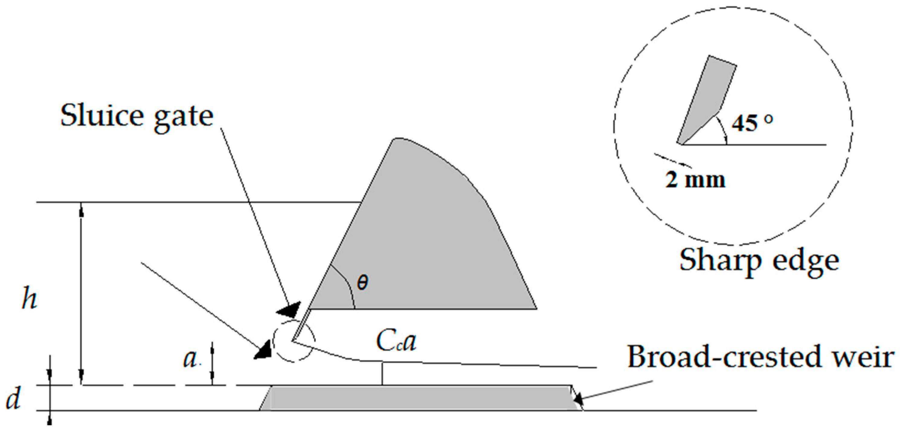
The scheme reported in Figure 1 shows that the weir was divided in two blocks, by means of two vertical planes with an opening of width b between them. A sluice gate set on the upstream wall could be closed, leaving an orifice of height a and width b, while h represents the upstream head. To make the flow free from any downstream influence, we used a broad-crested weir of height d at the bottom of the opening. The sluice gate had one sharp edge and the flow below it was free and completely aerated.
The study was first performed experimentally, when three series of tests were carried out with (and without) a broad-crested weir of height d = 20 mm located under the gate, at different values of the inclination angle θ of the weir upstream wall, that varied from 53.6° to 90°, and at different values of the shape ratio b/a and the relative opening a/h. Based on multiple regression, three expressions were found, relating the discharge coefficient with different parameters that characterized the phenomenon at hand.
Then, 27 numerical simulations were executed following the RANS approach to validate the numerical results against the experimental ones and to possibly investigate phenomena not caught by the experimental observation.
2.1. Dimensional Analysis
Considering the underflow of a sluice gate (Figure 1), we can assume a function F of the discharge Q and the other geometrical variables h, b, and a, as defined above, the angle between the weir upstream wall and the horizontal plane θ, the gravity acceleration g, the water density ρ, the kinematic viscosity ν the surface tension σ, and we can neglect the effect of the reservoir width, B, provided that it be sufficiently larger than b and the effect of the broad-crested weir, namely:
From the Π theorem, by selecting a, ρ, and g as basic variables, one has:
where Φ is a generic function, the parameter b/a is the shape ratio, a/h is the relative opening, and
are the Reynolds and Weber gate numbers, respectively.
When the liquid is the same and the temperature is constant, in the experimental set-up, Re and We depend on each other and vary with the gate opening only, as shown in [11], so we have to remove one of the two.
One obtains:
and, taking into account Equation (4), one can write:
Carrying out the tests in conditions where the viscosity and the surface tension do not affect the flow, Cd becomes a function of geometrical variables only:
2.2. Experimental Set-Up and Tests
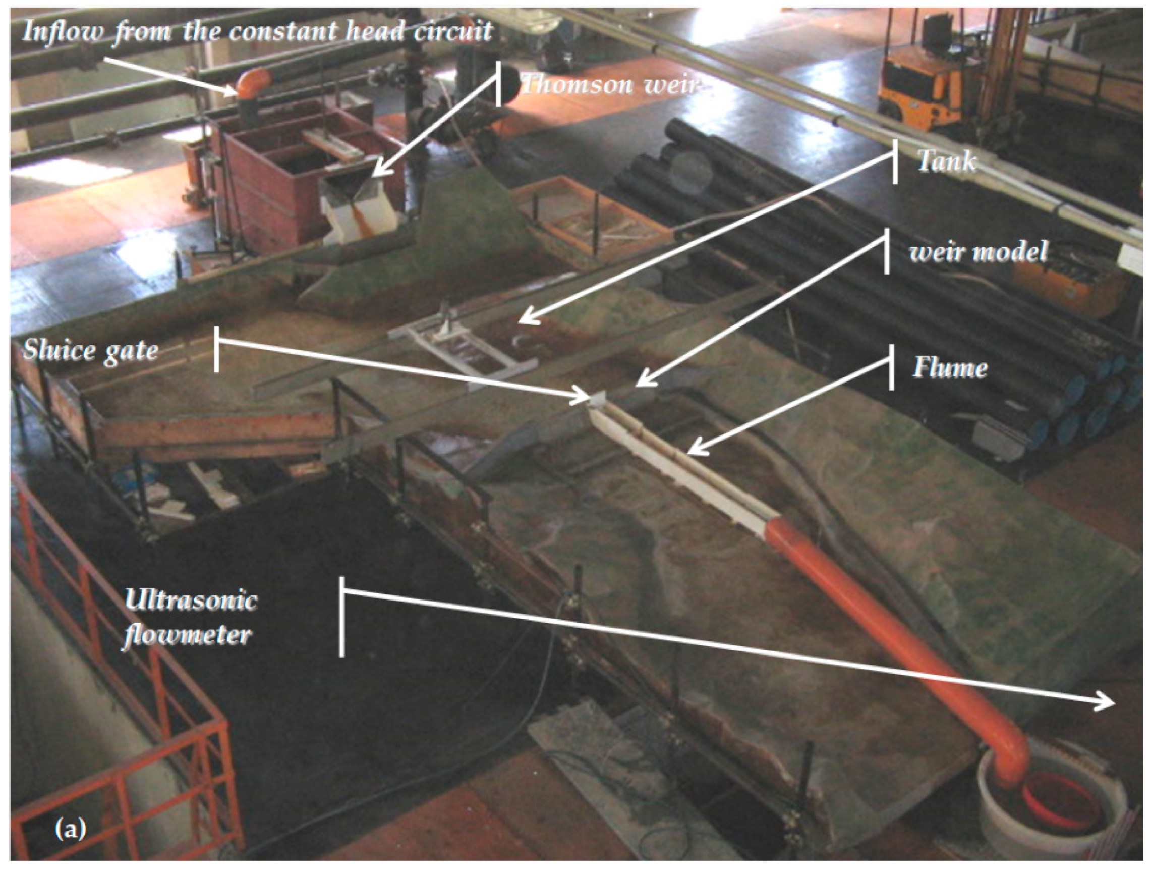
The experiments were conducted in a 1.20 m wide, 4.00 m long, and 0.25 m deep, horizontal, rectangular tank (Figure 2a,b) [12,13,14]. At its downstream end, a weir model 0.18 m high and 1.20 m wide was located. The orifice was created by dividing the weir in two parts in the middle by means of two vertical planes at a distance b from each other, and using a sluice gate level with the upstream wall. A PVC gate 10 mm thick was used, of which the crest was sharp-edged (Figure 1). A small flume of the same width as the gate width b was used downstream of the opening. For every series, three values of the gate widths b = 86, 106, and 142 mm were tested. The gate could be mounted with variable openings from the channel bottom. Three series of tests were carried out at different values of the weir upstream wall inclination angle θ, that varied from 53.6° to 90°. In the first series (Table 1) the angle θ was 63.4° (1.11 rad) and the gate opening was varied from a = 20 to 76 mm. In these tests, a PVC broad-crested weir of height d = 20 mm was located under the gate. In the second series (Table 2) three values of the weir angle θ = 56.3° (0.98 rad), 63.4° (1.11 rad), and 90° (1.57 rad) were considered, with gate openings a ≥ 50 mm. Also, in this case, the broad-crested weir was located under the gate. In the third series (Table 3) three values of the angle θ = 45° (0.78 rad), 63.4° (1.11 rad), and 90° (1.57 rad) were considered, and there were three values of the gate opening a = 50, 60 and 70 mm. For the latter series the broad-crested weir was not present.
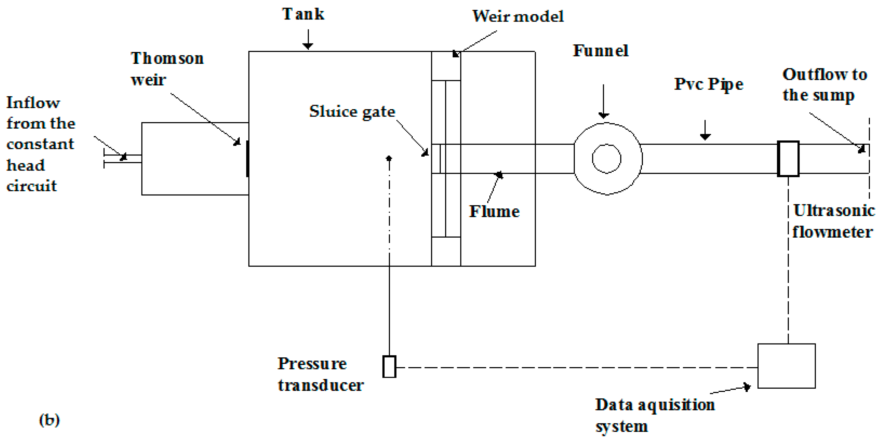
The flow was from the constant-head pipe circuit of the laboratory fed the tank. The discharge was measured by means of an ultrasonic flowmeter located on a PVC pipe downstream of the flume. A calibrated Thomson weir located upstream to the tank was used to check the ultrasonic flowmeter, when the flow was steady. During each test, the water level in the tank was recorded by means of a pressure transducer, with the tapping at 50 cm upstream from the orifice. A number of piezometric taps were in turn connected to the same pressure transducer [16], in order to get pressure measurements in 12 points of the tank. Once steady-state conditions were achieved, the free surface levels were measured by means of an electric point gauge with ± 0.5 mm reading accuracy, so allowing the control of the pressure transducer measurement. Both flow and free surface measurements were collected at a frequency of 50 Hz. In Table 1, Table 2 and Table 3 the values of the discharge coefficient is calculated using Equation (4).
2.3. Numerical Simulations
By means of numerical simulations the 27 runs of the Series 3 (Table 3) were carried out (considering the maximum values of h and Q) by solving the three-dimensional Reynolds-averaged Navier–Stokes (RANS) equations [17,18,19] in conservative form (the fluid is incompressible and viscous, Einstein summation convention applies to repeated indices, i, j = 1, 2, 3):
where is the fluid density, the water dynamic viscosity, the mean fluid pressure, are the mean velocity components, is the mean strain-rate tensor:
and the quantity is the Reynolds-stress tensor. The Reynolds-stresses are components of a symmetric, second-order tensor, where the diagonal components are normal stresses, while the off-diagonal elements are shear stresses. The Reynolds averaging procedure introduces six new unknown quantities (the six independent components of ) without providing additional equations. To close the system, the Boussinesq approximation has been used [20] and the eddy-viscosity has been expressed as a function of the turbulent kinetic energy (k) and the energy-dissipation rate (ε), leading to a two-equation turbulence model. In the present study, in order to establish a relationship between the Reynolds stresses and the mean flow field, the k-ε model [21] has been used.
For the execution of the calculations, the Flow-3D [22,23,24] finite-volume computational code has been used. In this code, the free-surface condition is handled with the VOF (volume of fluid) [25] method, that has extensively proven to be able to accurately track a wave interface [26,27]. The VOF method has been already used by several authors [24,26,27], always giving satisfactory results. This technique locates and tracks the free surface flow. To each fluid phase (hereinafter air and water), an individual fraction of the volume is associated, so that the indicator function can be expressed:
The two-phase flow can be assumed as a mixed fluid. Thus, the density and the dynamic viscosity can be defined:
in which the subscripts 1 and 2 indicate the two selected fluids (1 representing water and 2, air) and the volume–fraction function can be calculated by solving an advection equation for the velocity field:
The meshing technique does not induce mesh distortion during transients (a multi-block meshing technique can be also used to provide higher resolutions in the calculations, where needed). The time-marching procedure includes three main steps: (1) evaluation of the velocity in each cell using the initial conditions (or previous-time-step values) for the advective pressures (and/or other accelerations), on the basis of appropriate explicit approximations of the governing equations; (2) adjustment of the pressure in each cell to satisfy the continuity equation; and (3) updating of the fluid free surface to give the new fluid configuration based on the volume-of-fluid value in each cell. In the present calculations, the available solution scheme based on the generalized minimal residual (GMRES) method has been used. The fluid properties used in the simulations are reported in Table 4.
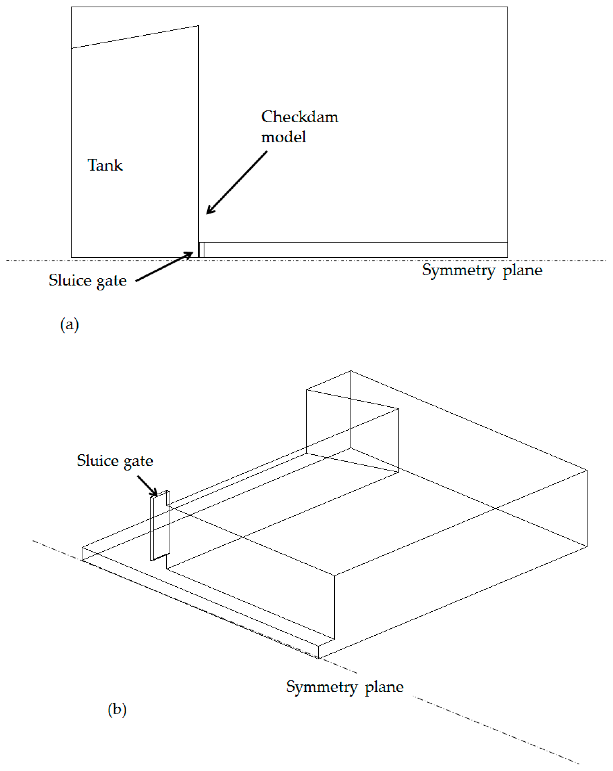
As for the numerical channel, a rectangular tank 0.496 m long and 0.400 m wide and a rectangular horizontal channel 0.300 m long has been considered. The computational domain extends 0.796 m × 0.400 m × 0.300 m along the x (streamwise), y (spanwise), and z (vertical) directions, respectively.
The origin of the coordinate system (x, y, z) is located at the lower-left corner of the computational domain, as shown in Figure 3a,b.
As for grid refinement, the unstructured computational mesh was refined through different steps, up to the point in which the comparisons of the computed results with those obtained by other authors became satisfactory. The final configuration of the computational grid is reported in Table 5.
The boundary conditions used for the computational domain are as follows: the no-slip (and zero wall-normal velocity) condition was imposed on the x–y bottom plane at the geometry external surface. To reduce the computational cost, the symmetry condition was imposed on the x–z left boundary plane and on the top of computational domain, on the y–z end-plane of the computing domain outflow conditions had been set, while the free-surface condition held at the fluid surface. On the y–z inlet plane, constant fluid depth was imposed, equal to that observed in the companion experimental test.
An initial condition of constant depth, equal to that measured experimentally and equal to that imposed at y–z plane, was imposed in the portion of domain upstream of the gate. The fluid moved with an instantaneous opening of the gate at t = 0.
A specially-assembled computing system was used for the simulations, that included 2 Intel Xeon 5660 exa-core multi-core processors (a total of 12 CPUs available), a maximum of 48 GB of RAM, and up to 1.8 TB of mass memory [28].
The simulations were executed using 16 processors. For parallel computing, the technique of the domain decomposition was adopted to split the geometry and the associated fields into segments. In this study, the “simple geometric decomposition” technique was used, in which the domain was broken into segments by direction. The elapsed computational time was about 6 hours of CPU time for each simulation.
The stability of the solution procedure was ensured by utilizing an adaptive time step with an initial value of 1 × 10⁻⁶ s, in conjunction with a mean Courant–Friedrichs–Lewy (CFL) number limit of 0.5.
3. Results and Discussion
Experimental Results
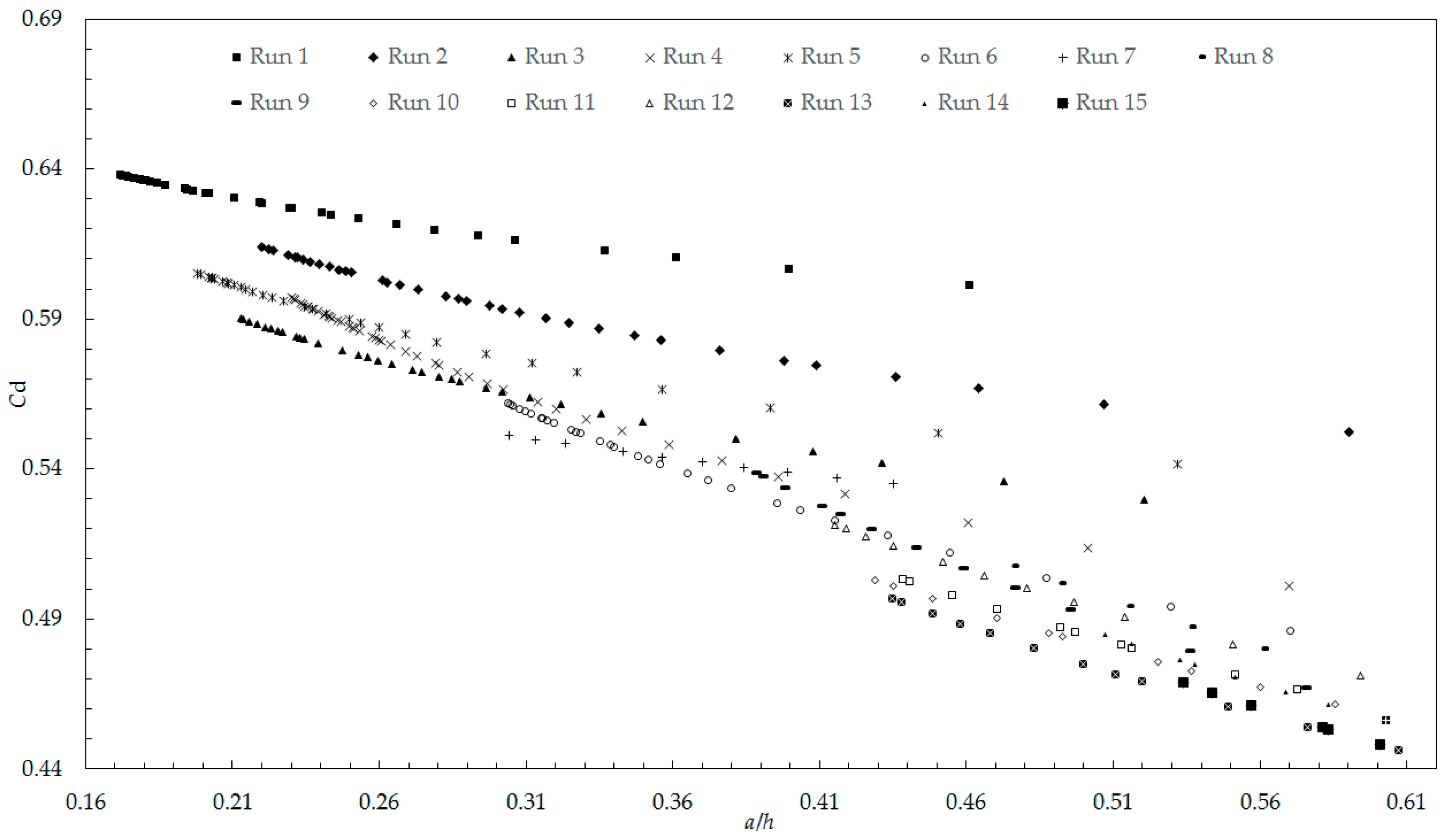
Figure 4 shows the values of the discharge coefficient as a function of the relative opening a/h with a weir inclination angle θ = 63.4° and with the aspect ratio b/a in the range 1.15–7.10 (Table 1).
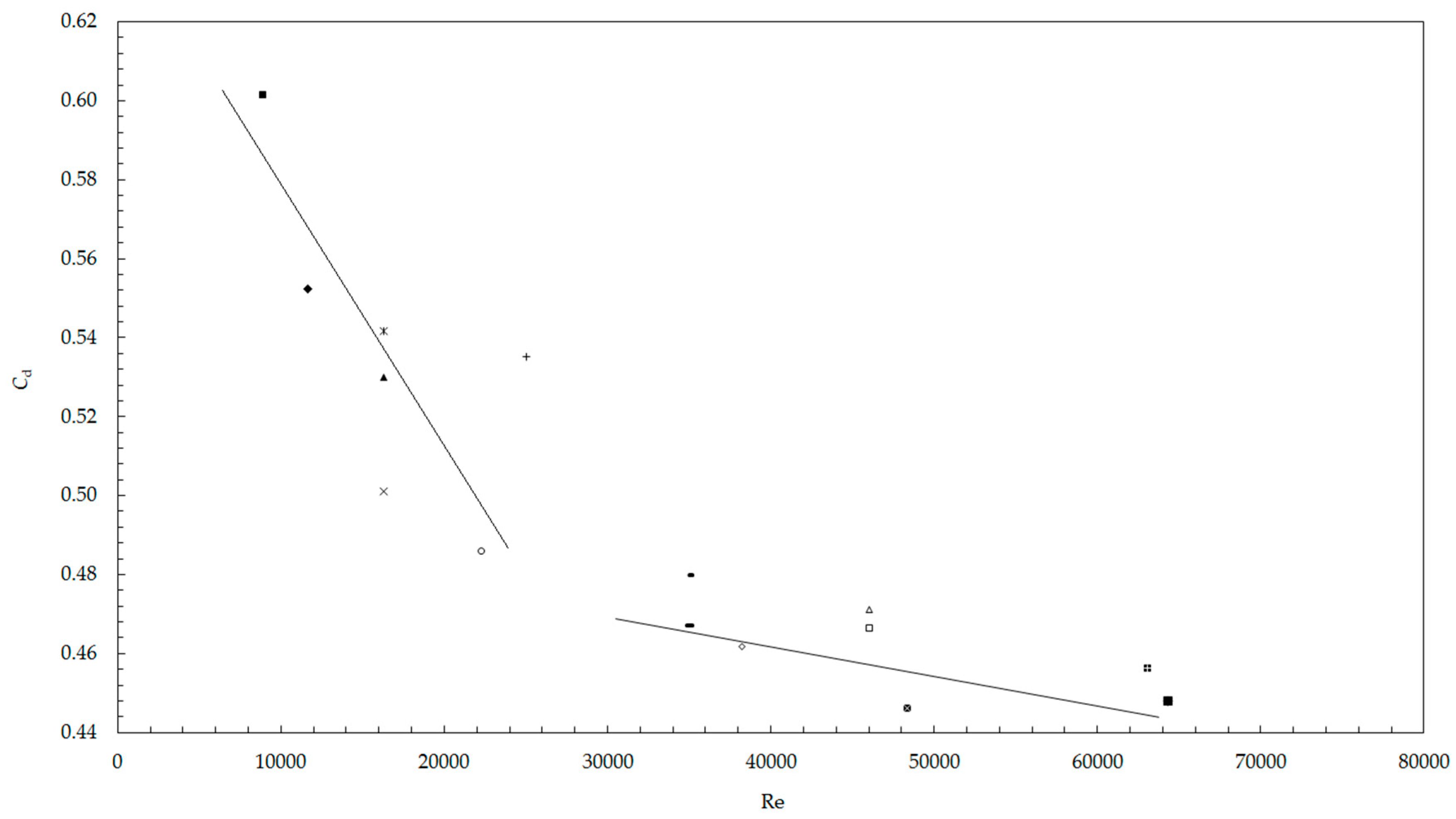
By following the method proposed by [5], of analyzing the minimum value of the discharge coefficient, (Cd,min), as a function of the Reynolds number, it was possible to identify a threshold value of this number, below which the viscosity substantially influenced the phenomenon.
The trend of the experimental data (Re and Cd,min), reported in Figure 5, showed that for values of Re ≤ 2.3 × 10⁴ the discharge coefficient varied rapidly, while for larger values it remained almost constant. Therefore, the results obtained highlight that, for a ≥ 4.0, We > 220, and Re > 2.3 × 10⁴, it is possible to neglect the effects of viscosity and surface tension, in accordance with what is reported in the literature [1,29].
To make explicit the functional relation between the discharge coefficient and the parameters on which it depends, a/h and b/a, for θ = 63.4°, a multiple regression was performed considering the values of the experimental variables (a, b, h, and Q) related to the 15 tests summarized in Table 1. To eliminate the scale effects due to the viscosity and to the surface tension [14], we considered, on the basis of the indications given by Figure 5, only the flow cases characterized by Re > 2.3 × 10⁴, therefore with a ≥ 4.0 cm (eight tests).
The following relationship was obtained:
valid for θ = 1.11 rad, a ≥ 4.0 and in the range of 0.30 ≤ a/h ≤ 0.61 and 1.15 ≤ b/a ≤ 3.55, with determination coefficient R2 = 0.927, maximum percent error emax = 3.6%, and average percent error eaverage = 1.3%.
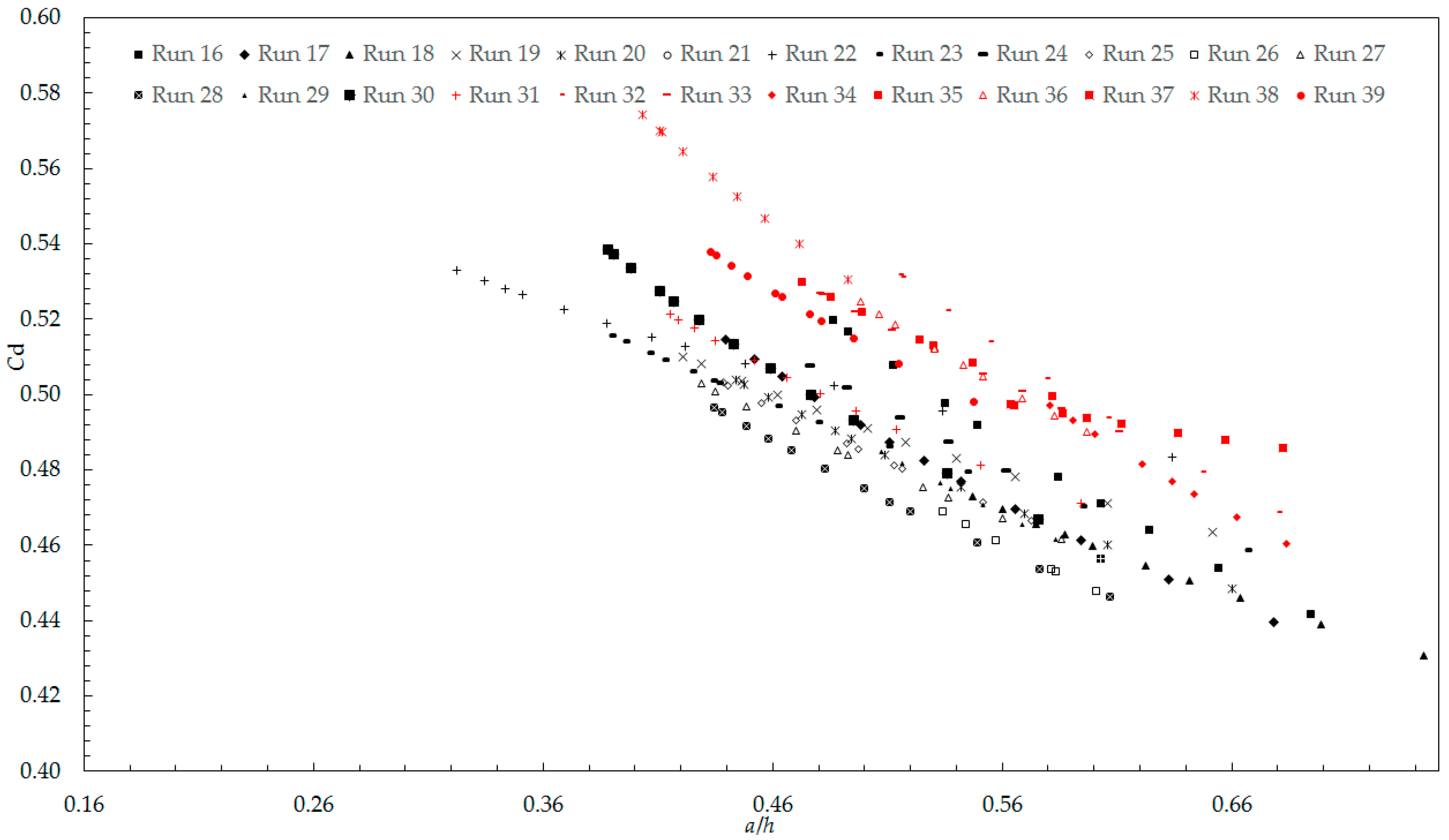
Figure 6 shows the values of the discharge coefficients as a function of the relative opening a/h for the weir inclination angle θ = 56.3°, 63.4°, and 90°, for the aspect ratio b/a = 1.15–2.84 with a ≥ 5.0 cm.
A multiple regression was performed considering the values of the experimental variables related to the 24 tests summarized in Table 2.
The following relationship was obtained:
valid for 0.98 rad ≤ θ ≤ 1.57 rad and a ≥ 5.0 and in the range of 0.32 ≤ a/h ≤ 0.75 and 1.15 ≤ b/a ≤ 2.84, with determination coefficient R2 = 0.870, maximum percent error emax = 3.8%, and average percent error eaverage = 1.0%.
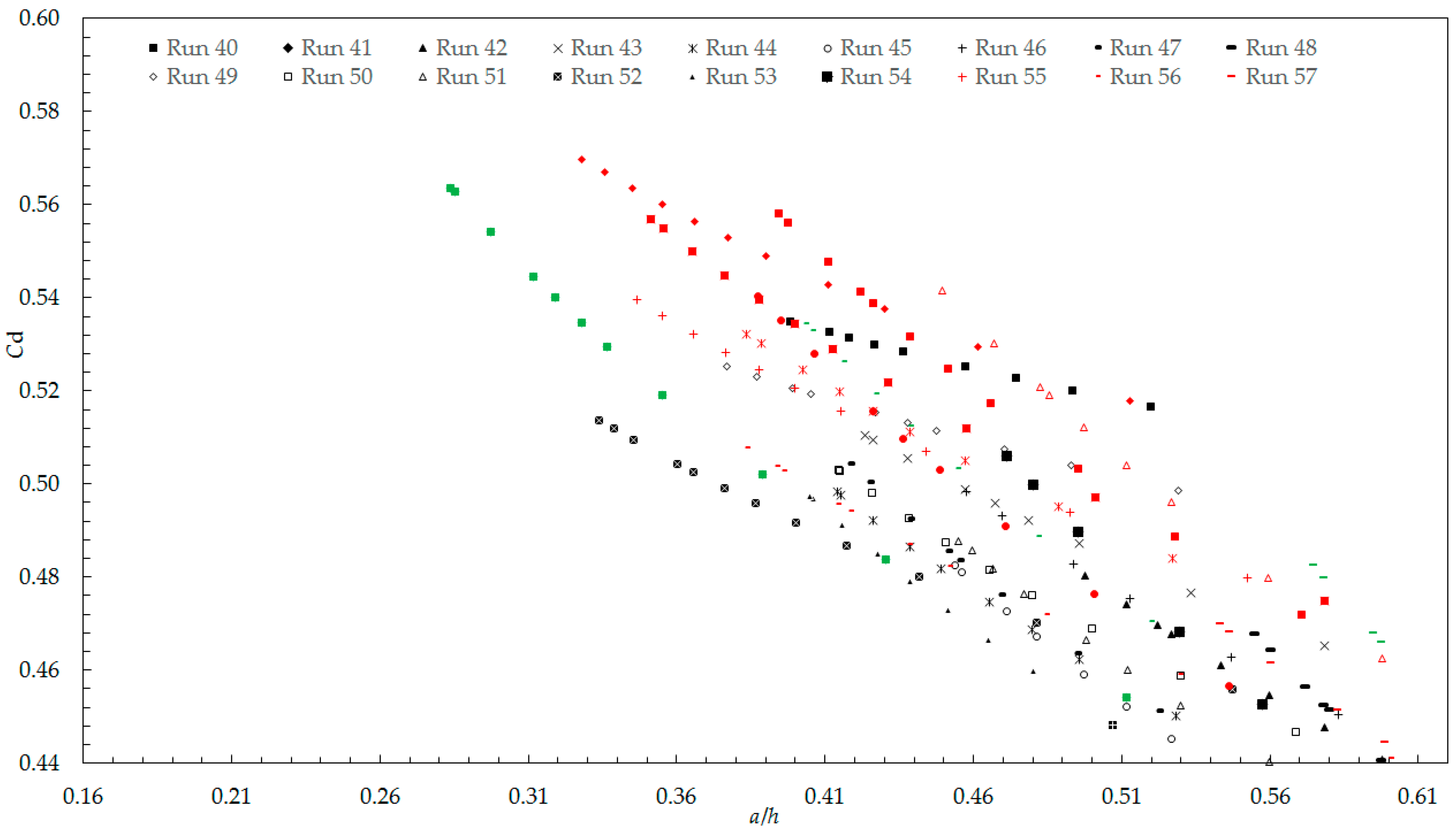
Figure 7 shows the values of the discharge coefficients as a function of the relative opening a/h for the weir inclination angle θ = 45.0°, 63.4°, and 90°, for the aspect ratio b/a = 1.23–2.84 and taking into account only the openings a ≥ 5.0 cm.
A multiple regression was performed considering the values of the experimental variables related to the 27 tests summarized in Table 3.
The following relationship was obtained:
valid for 0.78 rad ≤ θ ≤ 1.57 rad and a ≥ 5.0 and in the range of 0.30 ≤ a/h ≤ 0.60 and 1.23 ≤ b/a ≤ 2.84, with determination coefficient R2 = 0.73, maximum percent error emax = 9.6%, and average percent error eaverage = 2.8%.
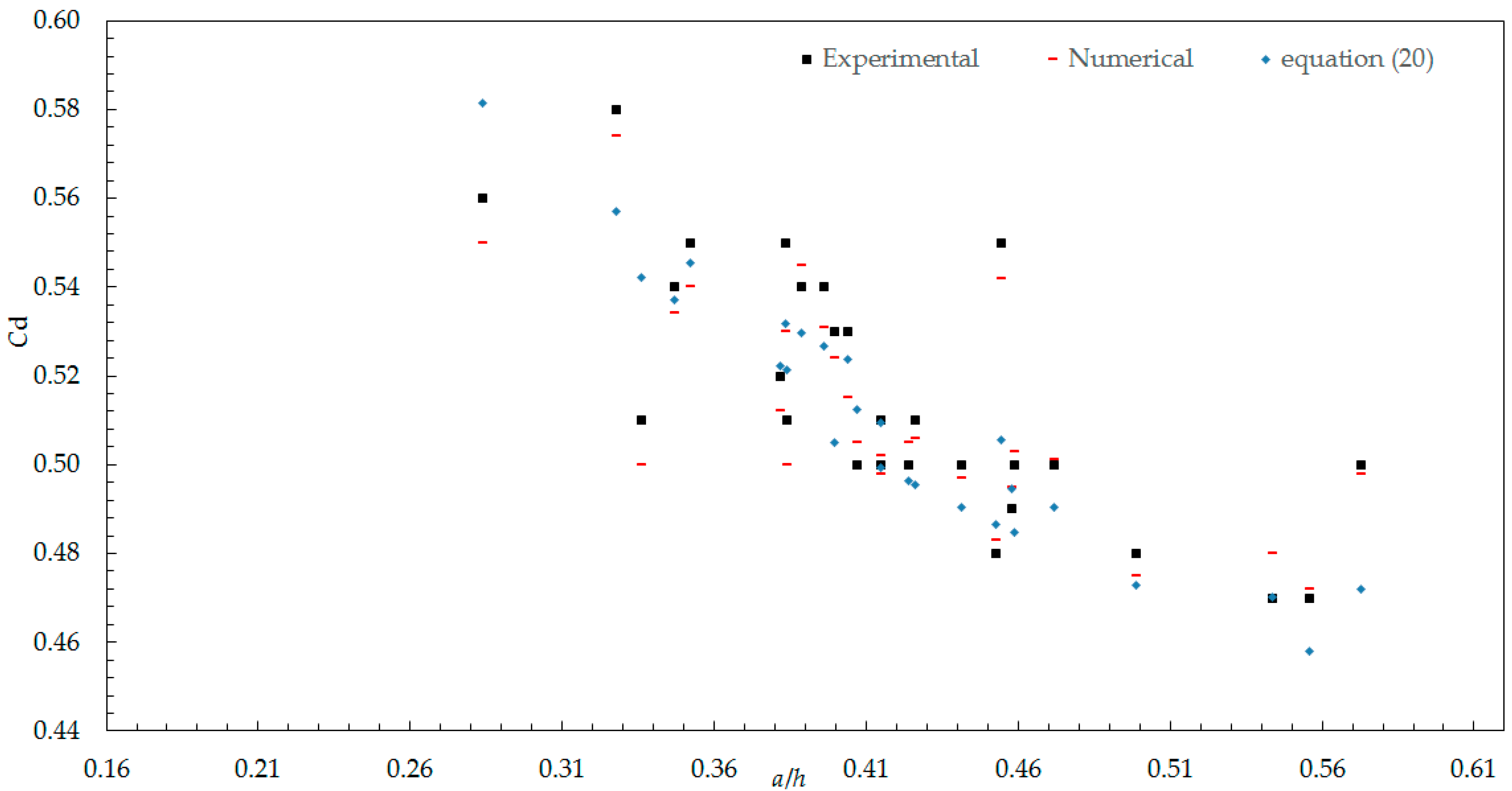
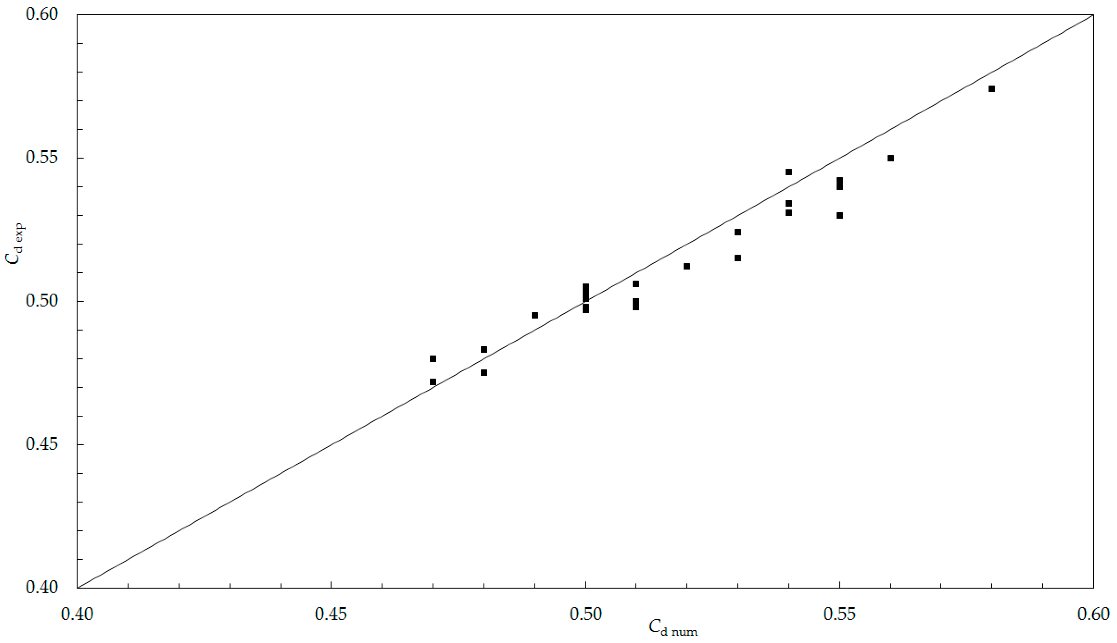
Comparison of the experimental values with the numerical results and the values given by Equation (20) of the discharge coefficients (Cd) for the 27 runs of Series 3, are shown in Figure 8, while Figure 9 illustrates a comparison of the numerical values of the discharge coefficients (Cd num) versus the experimental values of the discharge coefficients (Cd exp). By looking at the figures it is clear that the numerical simulation can be considered as an alternative approach to calculate the values of Cd, in particular in the cases in which performing laboratory tests is more difficult.
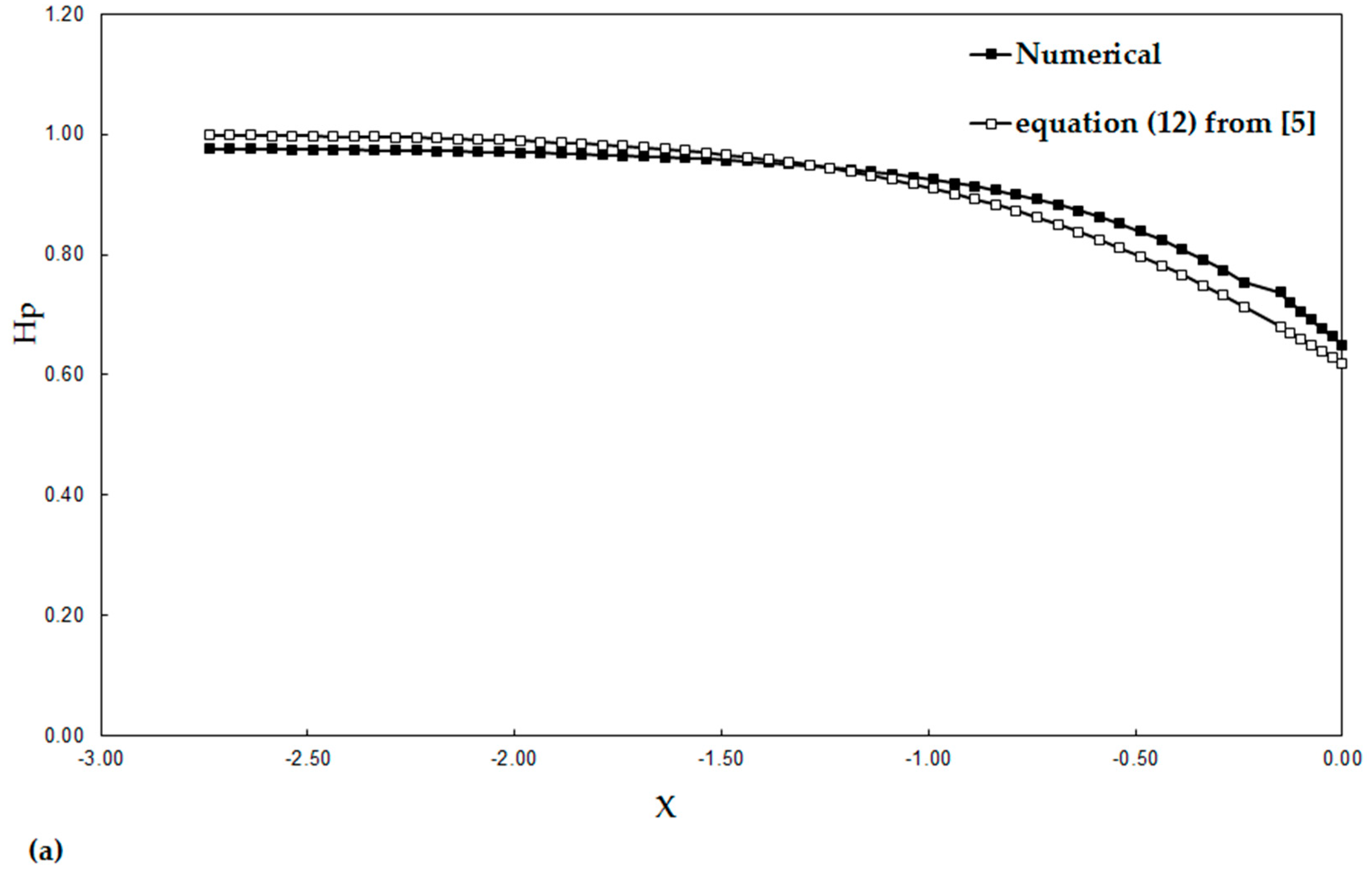
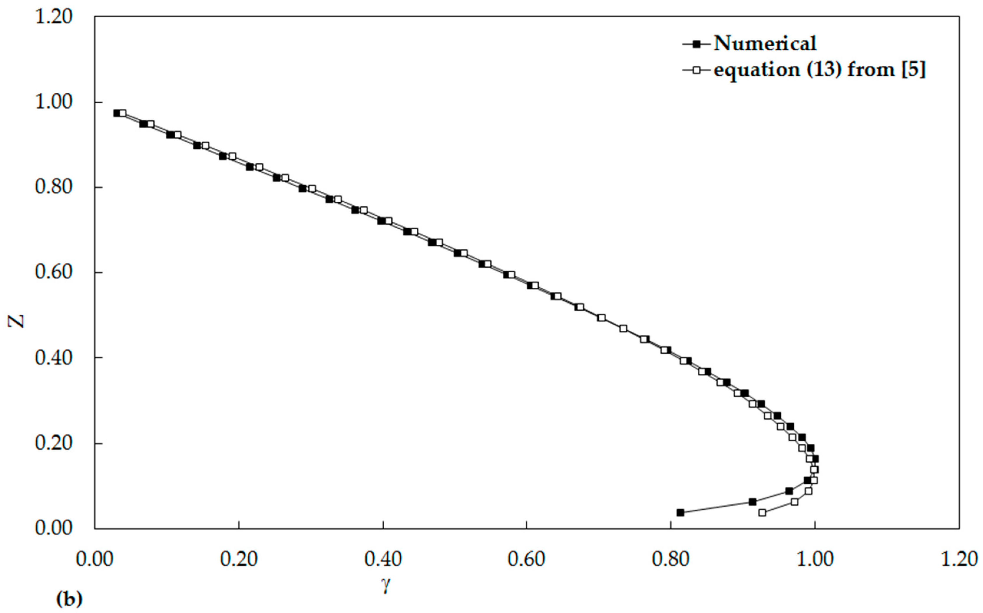
Figure 10a,b shows, for the Run 40 (Table 3), a comparison between numerical results and values given by Equation (12) of [5], the axial bottom pressure head Hp along the channel upstream from the gate, as a function of the dimensionless location X = x/a. Figure 10b shows a comparison between numerical and values given by the Equation (13) in [5] of the normalized gate pressure distribution γ(Z) as a function of dimensionless depth Z.
Figure 11 shows, for the case with angle θ of 90°, channel width b of 142 mm and gate opening a equal to 50 mm, a visual comparison between the experimental view and the numerical simulation of the symmetrical oblique waves located downstream from the gate. In particular Figure 11a shows the experimental observation of the waves, while Figure 11b shows the simulated numerical field (which is only the right side of Figure 11a). The fluid field obtained numerically (Figure 11b) is colored with the values of fluid pressure. It can be noticed how the symmetrical wave downstream from the gate is well represented.
4. Conclusions
In the present work laboratory experiments of discharge coefficients in the case of a gate set on the upstream wall of a weir at different inclination of the wall, allow us to identify the minimum value of the gate opening above which the scale effect due to viscosity is negligible. In this work, the underflow of a sluice gate in weir was analyzed and the effect of the gate slope and the side contraction was considered.
Based on multiple regression, three expressions were found, relating the discharge coefficient with different parameters that characterized the phenomenon at hand.
The first expression (Equation (18)), with a broad-crested weir, was valid only for θ = 63.4° and in the range of 0.30 ≤ a/h ≤ 0.61 and 1.15 ≤ b/a ≤ 3.55.
The second expression (Equation (19)), with a broad-crested weir, was valid for 56.3° ≤ θ ≤ 90° and a ≥ 5.0 cm and in the range of 0.32 ≤ a/h ≤ 0.75 and 1.15 ≤ b/a ≤ 2.84, and the last expression (Equation (19)), without a broad-crested weir, was valid for 45° ≤ θ ≤ 90° and a ≥ 5.0 cm and in the range of 0.30 ≤ a/h ≤ 0.60 and 1.23 ≤ b/a ≤ 2.84.
Our results may provide useful suggestions for those involved in sluice gate construction and management.
Furthermore 27 numerical simulations were carried out by means of the Reynolds-averaged Navier–Stokes equations to take into account the three-dimensionality of the phenomenon. The comparison between the experimental and numerical results revealed that the numerical code using the k-ε model in conjunction with the VOF method to track the free surface were sufficiently good to calculate the discharge coefficients, the bottom pressure head along the channel, and the gate axial distribution. The numerical model was also able to describe the oblique waves downstream from the gate showing that the proposed three-dimensional numerical procedure is a favorable option to correctly reproduce the phenomenon.
Author Contributions
A.L. and F.C. contributed in the design, performing, and result analysis of the laboratory tests; A.D. finalized the paper draft; G.A. and A.L. carried out the numerical simulations. All authors have read and agreed to the published version of the manuscript.
Funding
This research received no external funding.
Acknowledgments
The authors wish to thank Antonio Miglio for his contribution in performing the tests and in carrying out dimensional analysis.
Conflicts of Interest
The authors declare no conflict of interest.
References
- Sinniger, R.; Hager, W.H. Constructions Hydrauliques. Ecoulements Stationnaires; Presses Polytechniques Romandes; Traité de Génie Civil de l’Ecole polytechniques fédérale de Lausanne: Lausanne, Switzerland, 1988; Volume 15. [Google Scholar]
- Montes, J.S. Irrotational flow and real fluid effects under planar sluice gates. J. Hydraul. Eng. 1997, 123, 219–232. [Google Scholar] [CrossRef]
- Gentilini, B. Efflusso dalle luci soggiacenti alle paratoie piane inclinate e a settore. L’Energia Elettrica 1941, 18, 361–380. [Google Scholar]
- Rajaratnam, N.; Subramanya, K. Flow equation for the sluice gate. J. Irrig. Drain. Eng. 1967, 93, 167–186. [Google Scholar]
- Roth, A.; Hager, W.H. Underflow of standard sluice gate. Exp. Fluids 1999, 27, 339–350. [Google Scholar] [CrossRef]
- Rajaratnam, N. Free flow immediately below sluice gates. J. Hydraul. Div. ASCE 1977, 103, 345–351. [Google Scholar]
- Kim, D.G. Contraction and discharge coefficient of free flow past a sluice gate. In Proceedings of the Korea Water Resources Association Conference; Korea Water Resources Association: Seoul, Korea, 2005; pp. 1281–1282. [Google Scholar]
- Kim, D.G. Numerical Analysis of Free Flow Past a Sluice Gate. KSCE J. Civ. Eng. 2007, 11, 127–132. [Google Scholar] [CrossRef]
- Akoz, M.S.; Kirkgoz, M.S.; Oner, A.A. Experimental and numerical modeling of a sluice gate flow. J. Hydraul. Res. 2009, 47, 167–176. [Google Scholar] [CrossRef]
- Oskuyi, N.; Salmasi, F. Vertical Sluice Gate Discharge Coefficient. J. Civ. Eng. Urban. 2012, 2, 108–114. [Google Scholar]
- Raju, R. Scale Effects in Analysis of Discharge Characteristics of Weir and Sluice Gates; Kobus: Esslingen am Neckar, Germany, 1984. [Google Scholar]
- Lauria, A. Efflusso da luce di fondo di una traversa per laminazione delle piene. Analisi Sperimentale e Modellazione Numerica 3D. Ph.D. Thesis, Università della Calabria, Rende, Italy, 2008. [Google Scholar]
- Calomino, F.; Lauria, A.; Miglio, A.; Palma, G. Discharge coefficients for sluice gates in weir. In Proceedings of the Congress-International Association for Hydraulic Research, Venice, Italy, 1–6 July 2007. [Google Scholar]
- Calomino, F.; Lauria, A.; Miglio, A.; Palma, G. Determinazione sperimentale dei coefficienti d’efflusso da paratoie con diversa inclinazione per casse d’espansione. In Proceedings of the 30° Corso di aggiornamento in Tecniche per la difesa dall’inquinamento, Guardia Piemontese Terme (CS), Cosenza, Italy, June 2009; pp. 261–290. [Google Scholar]
- Calomino, F.; Lauria, A. 3-D Underflow of a Sluice Gate at a Channel Inlet; Experimental Results and CFD Simulations. J. Civ. Eng. Urban. 2014, 4, 501–508. [Google Scholar]
- Aristodemo, F.; Lauria, A.; Tripepi, G.; Rivera-Velasquéz, M.F.; Fallico, C. Smoothing of Slug Tests for Laboratory Scale Aquifer Assessment—A Comparison among Different Porous Media. Water 2018, 11, 1569. [Google Scholar] [CrossRef] [Green Version]
- Calomino, F.; Alfonsi, G.; Gaudio, R.; D’Ippolito, A.; Lauria, A.; Tafarojnoruz, A.; Artese, S. Experimental and numerical study of free-surface flows in a corrugated pipe. Water 2018, 10, 638. [Google Scholar] [CrossRef] [Green Version]
- D’Ippolito, A.; Lauria, A.; Alfonsi, G.; Calomino, F. Investigation of flow resistance exerted by rigid emergent vegetation in open channel. Acta Geophys. 2019, 67, 971–986. [Google Scholar] [CrossRef]
- Lauria, A.; Alfonsi, G. Numerical investigation of ski jump hydraulics. J. Hydraul. Eng. ASCE 2020, in press. [Google Scholar] [CrossRef]
- Wilcox, D.C. Turbulence Modeling for CFD; DCW Industries: La Cañada, CA, USA, 1998. [Google Scholar]
- Launder, B.E.; Spalding, D.B. The numerical computation of turbulent flows. Comput. Methods Appl. Mech. Eng. 1974, 3, 269–289. [Google Scholar] [CrossRef]
- FLOW SCIENCE. FLOW-3D User Manual: Excellence in Flow Modeling, Software Version 9.1; Flow Science, Inc.: Santa Fe, NM, USA, 2004. [Google Scholar]
- Alfonsi, G.; Lauria, A.; Primavera, L. Recent reults from analysis of flow structures and energy modes induced by viscous wave around a surface-piercing cylinder. Math. Probl. Eng. 2017. [Google Scholar] [CrossRef] [Green Version]
- Alfonsi, G.; Lauria, A.; Primavera, L. On evaluation of wave forces and runups on cylindrical obstacles. J. Flow Visual. Image Process. 2013, 20, 269–291. [Google Scholar] [CrossRef]
- Hirt, C.W.; Nichols, B.D. Volume of fluid (VOF) method for the dynamics of free boundaries. J. Comput. Phys. 1981, 39, 201–225. [Google Scholar] [CrossRef]
- Alfonsi, G.; Lauria, A.; Primavera, L. Proper orthogonal flow modes in the viscous-fluid wave-diffraction case. J. Flow Visual. Image Process. 2013, 20, 227–241. [Google Scholar] [CrossRef]
- Alfonsi, G.; Lauria, A.; Primavera, L. The field of flow structures generated by a wave of viscous fluid around vertical circular cylinder piercing the free surface. Procedia Eng. 2015, 116, 103–110. [Google Scholar] [CrossRef] [Green Version]
- Alfonsi, G.; Lauria, A.; Primavera, L. A study of the vortical structures past the lower portion of the Ahmed car model. J. Flow Visual. Image Process. 2013, 19, 81–95. [Google Scholar] [CrossRef]
- Novak, P.; Moffat, A.I.B.; Nalluri, C.; Narayanan, R. Hydraulic Structures; E & FN Spon: London, UK, 1996. [Google Scholar]
Figure 1.
Definition sketch of sluice gate (vertical section along the middle of the gate opening of width b), with notation.
Figure 1.
Definition sketch of sluice gate (vertical section along the middle of the gate opening of width b), with notation.

Figure 2.
(a) Physical model (view from downstream) and (b) definition sketch, with notation.


Figure 3.
Computational domain: (a) plan view and (b) 3D view from downstream.

Figure 4.
Discharge coefficients (Cd) versus a/h, Series 1.

Figure 5.
Discharge coefficients (Cd) versus Re, Series 1.

Figure 6.
Discharge coefficients (Cd) versus a/h, Series 2.

Figure 7.
Discharge coefficients (Cd) versus a/h, Series 3.

Figure 8.
Comparison of experimental, numerical and values given by Equation (20) of the discharge coefficients (Cd), Series 3.
Figure 8.
Comparison of experimental, numerical and values given by Equation (20) of the discharge coefficients (Cd), Series 3.

Figure 9.
Numerical vs. experimental discharge coefficients of Cd, Series 3.

Figure 10.
(a) Bottom pressure distribution comparison with Equation (12) given by [5] and (b) gate pressure distribution comparison with the Equation (13) given by [5].


Figure 11.
Symmetrical oblique waves downstream from the gate: (a) experimental and (b) numerical.


Table 1.
Experimental data Series 1.
| Run | θ (°) | a (mm) | b (mm) | h (mm) | Q (L/s) | b/a | a/h | Cd |
|---|---|---|---|---|---|---|---|---|
| 1 | 63.4 | 20 | 142 | 43.4 ÷ 116.4 | 1.58 ÷ 2.74 | 7.10 | 0.17 ÷ 0.46 | 0.60 ÷ 0.64 |
| 2 | 63.4 | 24 | 86 | 40.7 ÷ 109.1 | 1.02 ÷ 1.85 | 3.55 | 0.22 ÷ 0.60 | 0.55 ÷ 0.61 |
| 3 | 63.4 | 30 | 86 | 57.6 ÷ 140.9 | 1.45 ÷ 2.53 | 2.84 | 0.22 ÷ 0.53 | 0.52 ÷ 0.58 |
| 4 | 63.4 | 30 | 106 | 52.6 ÷ 130.4 | 1.62 ÷ 3.04 | 3.55 | 0.23 ÷ 0.57 | 0.50 ÷ 0.60 |
| 5 | 63.4 | 30 | 142 | 56.4 ÷ 151.4 | 2.43 ÷ 4.44 | 4.73 | 0.20 ÷ 0.53 | 0.54 ÷ 0.61 |
| 6 | 63.4 | 37 | 106 | 64.9 ÷ 121.8 | 2.15 ÷ 3.41 | 2.84 | 0.31 ÷ 0.58 | 0.48 ÷ 0.56 |
| 7 | 63.4 | 40 | 142 | 91.9 ÷ 131.4 | 4.08 ÷ 5.03 | 3.55 | 0.30 ÷ 0.44 | 0.54 ÷ 0.55 |
| 8 | 63.4 | 50 | 86 | 89.0 ÷ 105.0 | 2.73 ÷ 3.13 | 1.72 | 0.48 ÷ 0.56 | 0.48 ÷ 0.51 |
| 9 | 63.4 | 50 | 142 | 86.8 ÷ 128.8 | 4.33 ÷ 6.08 | 2.84 | 0.39 ÷ 0.58 | 0.47 ÷ 0.54 |
| 10 | 63.4 | 53 | 106 | 90.5 ÷ 123.6 | 3.45 ÷ 4.40 | 2.00 | 0.43 ÷ 0.59 | 0.46 ÷ 0.50 |
| 11 | 63.4 | 60 | 86 | 104.8 ÷ 136.9 | 3.45 ÷ 4.25 | 1.43 | 0.44 ÷ 0.57 | 0.47 ÷ 0.50 |
| 12 | 63.4 | 60 | 142 | 100.9 ÷ 144.5 | 5.65 ÷ 7.48 | 2.37 | 0.42 ÷ 0.59 | 0.47 ÷ 0.52 |
| 13 | 63.4 | 62 | 106 | 102.1 ÷ 142.6 | 4.15 ÷ 5.46 | 1.72 | 0.43 ÷ 0.61 | 0.45 ÷ 0.50 |
| 14 | 63.4 | 74 | 106 | 122.8 ÷ 145.9 | 5.55 ÷ 6.43 | 1.43 | 0.51 ÷ 0.60 | 0.46 ÷ 0.48 |
| 15 | 63.4 | 75 | 86 | 124.8 ÷ 140.5 | 4.52 ÷ 5.02 | 1.15 | 0.53 ÷ 0.60 | 0.45 ÷ 0.47 |
Table 2.
Experimental data Series 2.
| Run | θ (°) | a (mm) | b (mm) | h (mm) | Q (L/s) | b/a | a/h | Cd |
|---|---|---|---|---|---|---|---|---|
| 16 | 63.4 | 50 | 142 | 86.8 ÷ 128.0 | 4.30 ÷ 6.10 | 2.84 | 0.58 ÷ 0.39 | 0.47 ÷ 0.54 |
| 17 | 63.4 | 60 | 142 | 100.9 ÷ 144.5 | 5.60 ÷ 7.50 | 2.37 | 0.59 ÷ 0.41 | 0.47 ÷ 0.52 |
| 18 | 63.4 | 50 | 86 | 89.0 ÷ 104.8 | 2.70 ÷ 3.50 | 1.72 | 0.56 ÷ 0.48 | 0.48 ÷ 0.51 |
| 19 | 63.4 | 60 | 86 | 104.8 ÷ 136.9 | 3.50 ÷ 4.30 | 1.43 | 0.57 ÷ 0.44 | 0.47 ÷ 0.50 |
| 20 | 63.4 | 75 | 86 | 124.8 ÷ 140.5 | 4.50 ÷ 5.00 | 1.15 | 0.60 ÷ 0.53 | 0.45 ÷ 0.47 |
| 21 | 63.4 | 53 | 106 | 90.5 ÷ 123.6 | 3.50 ÷ 4.40 | 2.00 | 0.59 ÷ 0.43 | 0.46 ÷ 0.50 |
| 22 | 63.4 | 62 | 106 | 102.1 ÷ 142.6 | 4.20 ÷ 5.50 | 1.72 | 0.60 ÷ 0.43 | 0.46 ÷ 0.50 |
| 23 | 63.4 | 74 | 106 | 122.8 ÷ 143.3 | 5.60 ÷ 6.40 | 1.43 | 0.60 ÷ 0.51 | 0.46 ÷ 0.48 |
| 24 | 90.0 | 50 | 86 | 73.5 ÷ 97.0 | 2.40 ÷ 3.20 | 1.72 | 0.68 ÷ 0.51 | 0.47 ÷ 0.53 |
| 25 | 90.0 | 60 | 86 | 98.2 ÷ 124.8 | 3.50 ÷ 4.30 | 1.43 | 0.61 ÷ 0.48 | 0.49 ÷ 0.53 |
| 26 | 90.0 | 75 | 86 | 109.7 ÷ 129.1 | 4.40 ÷ 5.10 | 1.15 | 0.68 ÷ 0.58 | 0.46 ÷ 0.50 |
| 27 | 90.0 | 53 | 106 | 91.1 ÷ 112.1 | 3.80 ÷ 4.40 | 2.00 | 0.58 ÷ 0.47 | 0.50 ÷ 0.53 |
| 28 | 90.0 | 62 | 106 | 103.9 ÷ 124.5 | 4.60 ÷ 5.40 | 1.71 | 0.60 ÷ 0.50 | 0.49 ÷ 0.52 |
| 29 | 90.0 | 74 | 106 | 108.4 ÷ 131.2 | 5.60 ÷ 6.30 | 1.43 | 0.68 ÷ 0.56 | 0.40 ÷ 0.50 |
| 30 | 90.0 | 50 | 142 | 101.5 ÷ 123.9 | 5.30 ÷ 6.40 | 2.84 | 0.49 ÷ 0.40 | 0.53 ÷ 0.57 |
| 31 | 90.0 | 60 | 142 | 109.6 ÷ 138.6 | 6.20 ÷ 7.60 | 2.37 | 0.55 ÷ 0.43 | 0.50 ÷ 0.54 |
| 32 | 56.3 | 50 | 142 | 78.8 ÷ 155.0 | 4.30 ÷ 6.60 | 2.84 | 0.63 ÷ 0.32 | 0.48 ÷ 0.53 |
| 33 | 56.3 | 60 | 142 | 90.0 ÷ 153.9 | 5.20 ÷ 7.60 | 2.37 | 0.67 ÷ 0.39 | 0.46 ÷ 0.52 |
| 34 | 56.3 | 53 | 106 | 81.4 ÷ 125.9 | 3.30 ÷ 4.50 | 2.00 | 0.65 ÷ 0.42 | 0.46 ÷ 0.51 |
| 35 | 56.3 | 62 | 106 | 93.9 ÷ 139.7 | 4.00 ÷ 5.50 | 1.71 | 0.66 ÷ 0.44 | 0.45 ÷ 0.50 |
| 36 | 56.3 | 74 | 106 | 104.6 ÷ 143.8 | 4.90 ÷ 6.50 | 1.43 | 0.71 ÷ 0.51 | 0.43 ÷ 0.49 |
| 37 | 56.3 | 50 | 86 | 72.0 ÷ 102.8 | 2.30 ÷ 3.20 | 1.72 | 0.69 ÷ 0.49 | 0.44 ÷ 0.52 |
| 38 | 56.3 | 60 | 86 | 88.4 ÷ 136.5 | 3.00 ÷ 4.30 | 1.43 | 0.68 ÷ 0.44 | 0.44 ÷ 0.51 |
| 39 | 56.3 | 75 | 86 | 100.8 ÷ 137.1 | 3.90 ÷ 5.00 | 1.15 | 0.74 ÷ 0.55 | 0.43 ÷ 0.47 |
Table 3.
Experimental data Series 3 (see also [15]).
Table 3.
Experimental data Series 3 (see also [15]).
| Run | θ (°) | a (mm) | b (mm) | h (mm) | Q (L/s) | b/a | a/h | Cd |
|---|---|---|---|---|---|---|---|---|
| 40 | 90 | 50 | 142 | 74.9 ÷ 176.1 | 3.30 ÷ 7.40 | 2.84 | 0.67 ÷ 0.28 | 0.39 ÷ 0.56 |
| 41 | 90 | 60 | 142 | 115.5 ÷ 148.6 | 6.10 ÷ 7.70 | 2.36 | 0.52 ÷ 0.40 | 0.47 ÷ 0.53 |
| 42 | 90 | 70 | 142 | 87.7 ÷ 122.2 | 4.80 ÷ 7.50 | 2.03 | 0.80 ÷ 0.57 | 0.37 ÷ 0.50 |
| 43 | 90 | 50 | 106 | 66.6 ÷ 142.0 | 2.70 ÷ 4.90 | 2.12 | 0.75 ÷ 0.35 | 0.44 ÷ 0.55 |
| 44 | 90 | 60 | 106 | 79.3 ÷ 156.4 | 3.00 ÷ 6.00 | 1.76 | 0.76 ÷ 0.38 | 0.38 ÷ 0.55 |
| 45 | 90 | 70 | 106 | 89.7 ÷ 180.1 | 3.50 ÷ 7.60 | 1.51 | 0.78 ÷ 0.39 | 0.35 ÷ 0.54 |
| 46 | 90 | 50 | 86 | 65.9 ÷ 152.5 | 2.40 ÷ 4.20 | 1.72 | 0.76 ÷ 0.33 | 0.49 ÷ 0.58 |
| 47 | 90 | 60 | 86 | 73.9 ÷ 151.5 | 2.60 ÷ 4.80 | 1.43 | 0.81 ÷ 0.40 | 0.41 ÷ 0.54 |
| 48 | 90 | 70 | 86 | 87.4 ÷ 154 | 3.10 ÷ 5.50 | 1.23 | 0.80 ÷ 0.45 | 0.40 ÷ 0.55 |
| 49 | 63.4 | 50 | 142 | 46.1 ÷ 144.06 | 3.30 ÷ 6.30 | 2.84 | 1.08 ÷ 0.35 | 0.48 ÷ 0.54 |
| 50 | 63.4 | 60 | 142 | 99.9 ÷ 156.3 | 5.00 ÷ 7.60 | 2.36 | 0.60 ÷ 0.38 | 0.42 ÷ 0.51 |
| 51 | 63.4 | 70 | 142 | 46.1 ÷ 128.8 | 4.20 ÷ 7.40 | 2.03 | 1.52 ÷ 0.54 | 0.45 ÷ 0.47 |
| 52 | 63.4 | 50 | 106 | 76.5 ÷ 148.7 | 2.80 ÷ 4.70 | 2.12 | 0.65 ÷ 0.34 | 0.43 ÷ 0.51 |
| 53 | 63.4 | 60 | 106 | 82.7 ÷ 147.5 | 3.10 ÷ 5.50 | 1.76 | 0.72 ÷ 0.41 | 0.38 ÷ 0.50 |
| 54 | 63.4 | 70 | 106 | 92.1 ÷ 148.4 | 3.50 ÷ 6.10 | 1.51 | 0.76 ÷ 0.47 | 0.36 ÷ 0.50 |
| 55 | 63.4 | 50 | 86 | 64.5 ÷ 131 | 2.30 ÷ 3.60 | 1.72 | 0.77 ÷ 0.38 | 0.48 ÷ 0.52 |
| 56 | 63.4 | 60 | 86 | 80.7 ÷ 144.6 | 2.60 ÷ 4.30 | 1.43 | 0.74 ÷ 0.41 | 0.39 ÷ 0.51 |
| 57 | 63.4 | 70 | 86 | 90.4 ÷ 152.8 | 3.00 ÷ 5.10 | 1.23 | 0.77 ÷ 0.46 | 0.37 ÷ 0.49 |
| 58 | 45 | 50 | 142 | 62.1 ÷ 109 | 3.00 ÷ 5.20 | 2.84 | 0.80 ÷ 0.46 | 0.38 ÷ 0.50 |
| 59 | 45 | 60 | 142 | 93.8 ÷ 141.5 | 4.70 ÷ 7.20 | 2.36 | 0.64 ÷ 0.42 | 0.41 ÷ 0.50 |
| 60 | 45 | 70 | 142 | 85.7 ÷ 125.9 | 4.30 ÷ 7.40 | 2.03 | 0.82 ÷ 0.56 | 0.33 ÷ 0.47 |
| 61 | 45 | 50 | 106 | 65.1 ÷ 117.3 | 2.50 ÷ 4.10 | 2.12 | 0.77 ÷ 0.43 | 0.42 ÷ 0.51 |
| 62 | 45 | 60 | 106 | 75.7 ÷ 144.62 | 2.90 ÷ 5.40 | 1.76 | 0.79 ÷ 0.41 | 0.38 ÷ 0.50 |
| 63 | 45 | 70 | 106 | 86.3 ÷ 154.6 | 3.40 ÷ 6.30 | 1.51 | 0.81 ÷ 0.45 | 0.35 ÷ 0.48 |
| 64 | 45 | 50 | 86 | 66.1 ÷ 125.1 | 2.50 ÷ 3.50 | 1.72 | 0.76 ÷ 0.40 | 0.50 ÷ 0.53 |
| 65 | 45 | 60 | 86 | 76.2 ÷ 136.0 | 2.50 ÷ 4.20 | 1.43 | 0.79 ÷ 0.44 | 0.40 ÷ 0.50 |
| 66 | 45 | 70 | 86 | 86.9 ÷ 140.3 | 2.90 ÷ 4.80 | 1.23 | 0.81 ÷ 0.50 | 0.37 ÷ 0.48 |
Table 4.
Fluid properties used in the simulations.
| Air Density | Water Density | Air Kinematic Viscosity | Water Kinematic Viscosity |
|---|---|---|---|
| 1.225 kg/m3 | 1000 kg/m3 | 1.48 × 10⁻⁵ m2/s | 1.0 × 10⁻⁶ m2/s |
Table 5.
Characteristic parameters of the computational grid.
| Nx | Ny | Nz | Δx_min (m) | Δy_min (m) | Δz_min (m) |
|---|---|---|---|---|---|
| 124 | 100 | 150 | 0.002 | 0.002 | 0.002 |
© 2020 by the authors. Licensee MDPI, Basel, Switzerland. This article is an open access article distributed under the terms and conditions of the Creative Commons Attribution (CC BY) license (http://creativecommons.org/licenses/by/4.0/).
Share and Cite
MDPI and ACS Style
Lauria, A.; Calomino, F.; Alfonsi, G.; D’Ippolito, A. Discharge Coefficients for Sluice Gates Set in Weirs at Different Upstream Wall Inclinations. Water 2020, 12, 245. https://doi.org/10.3390/w12010245
AMA Style
Lauria A, Calomino F, Alfonsi G, D’Ippolito A. Discharge Coefficients for Sluice Gates Set in Weirs at Different Upstream Wall Inclinations. Water. 2020; 12(1):245. https://doi.org/10.3390/w12010245
Chicago/Turabian StyleLauria, Agostino, Francesco Calomino, Giancarlo Alfonsi, and Antonino D’Ippolito. 2020. "Discharge Coefficients for Sluice Gates Set in Weirs at Different Upstream Wall Inclinations" Water 12, no. 1: 245. https://doi.org/10.3390/w12010245
Note that from the first issue of 2016, this journal uses article numbers instead of page numbers. See further details here.