Uncertainty Analysis of Spatiotemporal Models with Point Estimate Methods (PEMs)—The Case of the ANUGA Hydrodynamic Model


Department of Bioenvironmental Systems Engineering, National Taiwan University, Taipei 10617, Taiwan
*
Author to whom correspondence should be addressed.
†
Current address: National Taiwan University, Department of Bioenvironmental Systems Engineering, No. 1, Section 4, Roosevelt Rd, Da’an District, Taipei City 10617, Taiwan.
Water 2020, 12(1), 229; https://doi.org/10.3390/w12010229
Submission received: 28 November 2019
/
Revised: 2 January 2020
/
Accepted: 9 January 2020
/
Published: 14 January 2020
(This article belongs to the Special Issue Advances in Hydrologic Forecasts and Water Resources Management )
Abstract
:Practitioners often neglect the uncertainty inherent to models and their inputs. Point Estimate Methods (PEMs) offer an alternative to the common, but computationally demanding, method for assessing model uncertainty, Monte Carlo (MC) simulation. PEMs rerun the model with representative values of the probability distribution of the uncertain variable. The results can estimate the statistical moments of the output distribution. Hong’s method is the specific PEM implemented here for a case study that simulates water runoff using the ANUGA model for an area in Glasgow, UK. Elevation is the source of uncertainty. Three realizations of the Sequential Gaussian Simulation, which produces the random error fields that can be used as inputs for any spatial model, are scaled according to representative values of the distribution and their weights. The output from a MC simulation is used for validation. A comparison of the first two statistical moments indicates that Hong’s method tends to underestimate the first moment and overestimate the second moment. Model efficiency performance measures validate the usefulness of Hong’s method for the approximation of the first two moments, despite the method suffering from outliers. Estimation was less accurate for higher moments but the moment estimates were sufficient to use the Grams-Charlier Expansion to fit a distribution to them. Regarding probabilistic flood-inundation maps, Hong’s method shows very similar probabilities in the same areas as the MC simulation. However, the former requires just three 11-minute simulation runs, rather than the 500 required for the MC simulation. Hong’s method therefore appears attractive for approximating the uncertainty of spatiotemporal models.
1. Introduction
Flood inundation, in its many forms, is one the most devastating types of natural disaster for civilization [1]. Floods are involved in the majority of fatalities associated with natural disasters [2] and cause severe economic damage by disrupting and destroying processes within the society and economy. The socio-economic impact of flood inundations has given rise to studies on the subject receiving widespread interest. Flood-risk assessments are in particular focus and are legally required in some parts of the world, for example in the European Directive on the Assessment and Management of Flood Risks [3].
Maps are one of the best ways to present the spatial distribution of uncertainty and risk. Flood-risk maps are event-based and show the probability of the occurrence and consequences of a flood [1]. The process of producing flood-risk maps involves floodplain mapping and uncertainty analysis. Floodplain maps are generated by a deterministic approach using either empirical, hydrodynamic or simplified-conceptual models [4,5,6,7,8,9]. Historical flood data is employed to validate models and calibrate their parameters [10]. Despite a notable research effort in recent decades, deterministic models remain afflicted by uncertainty [9]. This is in part because the models are assumed to be a comprehensive representation of the relevant physical processes and their relationship to water flow, and in part because they are assumed to use an optimal set of parameters. The issue is further compounded because uncertainty is likely to be non-stationary. Practitioners such as environmental agencies, river basin authorities and engineering consultancies often fail to fully invest the effort required for the detailed setting up of model and lack the computational resources required to solve the physical models [1]. This means that, in practice, additional uncertainty can be introduced to flood inundation modelling by the application of simplified, conceptual models in a deterministic way.
Realistically evaluating the risk of flood events and planning countermeasures therefore requires probabilistic floodplain maps, which are produced from ensemble simulations, like sensitivity analysis, of deterministic models [1]. The probabilistic approach is also more robust concerning the non-stationary aspect of uncertainty because of the many simulations that use a diverse set of data and parameters. Despite awareness of the benefits of this approach, Di Baldassarre et al. [1] claims that practitioners rarely apply probabilistic methods because of a slow rate of knowledge transfer and their familiarity with deterministic results. The authors further conclude there is a lack of a coherent terminology, a systematic approach and mature guidance for the use of probabilistic methods in hydrological analyses.
Reliability engineering has made a major contribution to uncertainty analysis. For one-dimensional models, several approaches can be used to quantify uncertainty. These include the First-Order Second-Moment (FOSM) method [11], Monte Carlo (MC) simulations [12], the Moment method [13], the spectral method [14], the Mellin transformation [15,16] and Point Estimate Methods (PEMs) [17,18,19,20,21,22].
Two-dimensional models are complicated by the need to consider spatial variability, which is handled by random field theories. Random fields can be generated in many ways [23] and serve as input for MC simulations which are common in uncertainty analysis, though very demanding in terms of computational resources. The study by Aerts et al. [24] is a good example: the researchers attempt to optimally locate and design a ski run while considering the uncertainty arising from an uncertain Digital Elevation Map (DEM). The uncertainty is analyzed by a MC simulation, the distinct DEM realizations are derivatives of random error fields, and the error values are the result of measurements at ground control locations. The measured differences are then analyzed for their spatial structure in the form of a variogram. Kriging is used as part of a Sequential Gaussian Simulation (SGS) [25,26,27]. SGS is a method of generating random fields to interpolate the non-measured errors between the ground control locations.
The popularity of MC simulations is illustrated by their continuous development. This development has led to various stratified sampling methods [28,29] that reduce the computational burden of MC, for example, Latin Hypercube Sampling [30,31,32]. Another improvement was the combination of MC with the Markov Chain process [33,34,35]. A useful implementation of MC can be found in the work by Feinberg and Langtangen [36].
Suchomel et al. [37] present a hybrid method combining the FOSM with random fields. Although the method can only consider uncorrelated uncertain variables, spatial correlation is accounted for by spatial averaging, which thus implies a variance reduction. The method was implemented as a finite element model.
In hydrology, uncertainty is commonly quantified by sensitivity analysis [9]. This involves perturbing within feasible limits variables and parameters–either individually and gradually (local) or simultaneously and randomly–and then assessing the effects on the outputs and any interactions.
The Generalized Likelihood Uncertainty Estimation (GLUE) is based on a Bayesian approach [1]. Similar to MC, GLUE requires several model realizations using random samples of the parameter in focus. The realizations are subsequently distinguished into behavioral and non-behavioral groups. The outputs (e.g., the extent of flood inundation) are merged using Bayesian equations to result in a distributed probability profile. GLUE is less rigorous and requires the user to make many choices, increasing the potential for methodological errors [9].
A probabilistic modelling approach usually involves repeated runs of deterministic models using samples from across the range of parameters and available data. The purpose is to approximate the probability distribution of the output. For users with scarce computational resources, simplified conceptual methods are often more convenient than physics-based models.
The purpose of this study is to expand the application of PEMs to uncertainty analysis of spatiotemporal models and to develop a convenient way to produce probabilistic inundation maps.
2. Materials and Methods
This section explains the modelling approach and data used in this study. First, the ANUGA inundation spatial model [38,39] is briefly explained. The MC approach is subsequently discussed and this is followed by an introduction to Hong’s PEM [20]. Furthermore, the expansion of PEM to two-dimensional space is clarified. Finally, the section concludes by describing a case study and its data set.
2.1. ANUGA
ANUGA is developed by the Australian National University (ANU) and Geoscience Australia (GA). The fluid dynamics of ANUGA is implemented using a finite volume approach to solve the Shallow Water Wave Equations. The simulation domain is partitioned into a mesh of triangular cells. The governing Shallow Water Wave Equations are solved at the centroid of the cell and thus provide water depth and horizontal momentum over time. ANUGA is capable of simulating the wetting and drying process when water enters and leaves a cell. It can therefore approximate the flow onto a beach, dry land and around structures such as buildings. Discontinuities, such as hydraulic jumps, are accommodated by the finite-volume implementation. A scenario set-up requires the domain’s geometry, initial water level and boundary conditions. The drivers of the system in the inundation model, like rainfall, abstraction and culverts, are designed as operators and are also required to set up the scenario. The mesh generator can be used interactively to help the user to tailor the domain’s geometry. Mesh triangles are symbolically tagged to indicate boundary regions or regions with different parameters, such as the Manning friction coefficients. ANUGA is mainly written in the Python programming language, which allows for flexible usage [39]. Computationally intensive components are executed as C routines by the means of Python’s numerical module Numpy. The approach has been validated by adequately modelling various inundation problems [40,41].
2.2. Monte Carlo Simulation
MC simulation involves running a simulation many times with different random samples from the probability distribution of an uncertain input variable to obtain a numerical probability distribution of the output variable [24]. MC is very commonly used in uncertainty quantification to capture a system’s natural variability [12,42,43]. The MC simulation serves as benchmark in this study to test the accuracy of the spatially implemented PEM. The outcome of MC is currently the best approximation to the “ground truth” of a stochastic system.
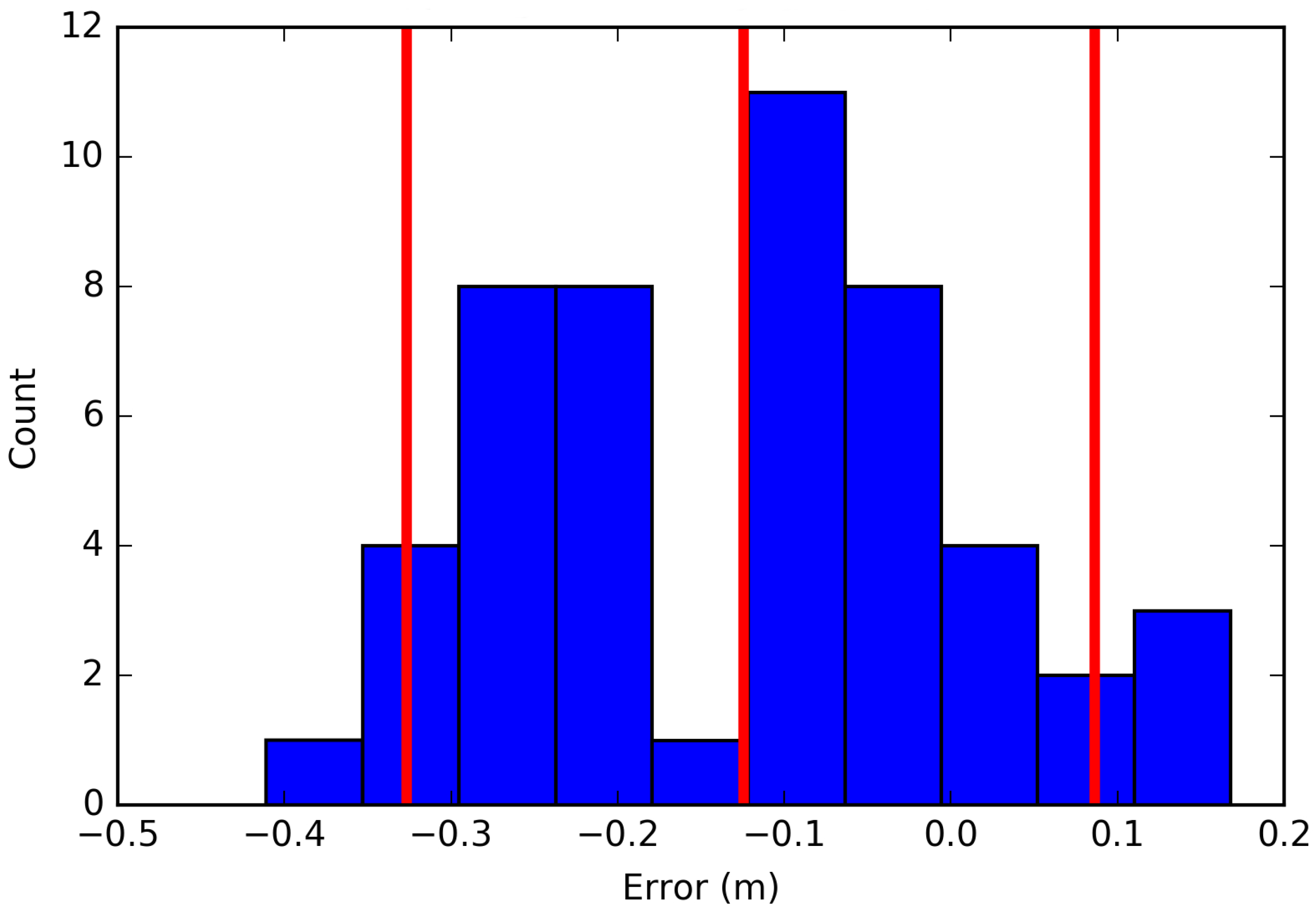
Distinct spatial realizations of the input variable in question (ground elevation) are produced by a SGS. Random error fields induce noise into the DEM data to derive distinct realizations. The error values originate from the differences between the original data set and the ground control data set at 50 locations. Figure 1 shows the histogram of the elevation error, which displays a non-normal form. Error values were interpolated by Ordinary Kriging to obtain error values for the whole spatial domain. Because Kriging provides an estimate of a variable’s mean and standard deviation, the variable can be represented as a random variable according to a Gaussian distribution. However, Figure 1 shows that the errors are not normally distributed, and thus need to be normalized by the means of normal score transformation [44].
The MC approach requires many simulation runs. Accordingly, 500 were carried out for this study, requiring 500 distinct realizations of the random error field. The first step was to create the same number of random paths visiting every grid cell. Following these paths, the error value for each non-ground control cell was interpolated according to neighboring cells in relationship to the variogram. Because each path is different, the error value of each cell differed slightly from those around it. The mean and standard deviation of the Kriging enabled a random selection from a normal distribution. SGS was conducted by a Python library using the mean of the High Performance Geostatistics Library [45]. Subsequently, the error values were back-transformed into the original distribution [44]. The advantage of using Kriging was weighting the influence of the neighboring cells according to the semivariogram permitted the spatial structure to be respected.
2.3. Hong’s Point Estimate Method
2.3.1. Theory
The core idea of the PEM is to calculate the statistical moments of the output variables. The moments are derived from several realizations of a deterministic model using representative values of the uncertain variable as an input. The purpose is to approximate the probability distribution of the model’s output variable, which is related to the probability distribution of the uncertain input variables. The process only requires a few statistical moments of the input variables to be known. The derivation of PEM assumes that the rth moment of the output variable is the integral of the evaluation function with the random input variables over their domains with respect to their joint distribution functions. The equations of the representative values and weights are the products of expanding this function by Taylor series at various points of the variable distributions. The original PEM was proposed by Rosenblueth [21], but this has since proved to be too inefficient because it requires model evaluations, where m is the number of uncertain variables. Thus, the refinement suggested by Hong [20], which is a is a PEM scheme, was used.
Although this study considers only one variable (elevation), the set of random variables is defined as . Therefore, to compute the statistical moments of the output requires just three simulation runs, one for each representative input value, k. The first four statistical central moments (mean, variance, skewness and kurtosis) were used to approximate the distribution of the uncertain variable and thus compute the location of the representative values.
The locations of the representative values for each uncertain variable, i, in standardized space, , were computed by Equation (1) based on the skewness, , and kurtosis, , of the uncertain variable.
Subsequently, the standardized location was transformed using the mean, , and standard deviation, , of the uncertain variable to its original space, , by Equation (2). The representative value was the mean value of the variable.
Based on the standardized values for location, skewness and kurtosis, the weights for the representative values, , were then calculated by Equation (3).
The weight determines the proportion of impact that each evaluation of the model at the location of the representative value has on the statistical moment of the output variable. The rth statistical moment of a function of m random variables, Z, was then approximated by Equation (4).
2.3.2. Spatial Implementation of PEM
Similar to the MC approach, the spatial implementation also relies on random error fields. Instead of 500 error fields, this study only uses error fields, i.e., three, given that only one uncertain variable is considered. The three error fields were produced by the SGS process. Hong’s method was then used to determine the representative values of the distribution as described by Equations (1) and (2). Figure 1 shows the histogram of the errors with the locations of the representative values.
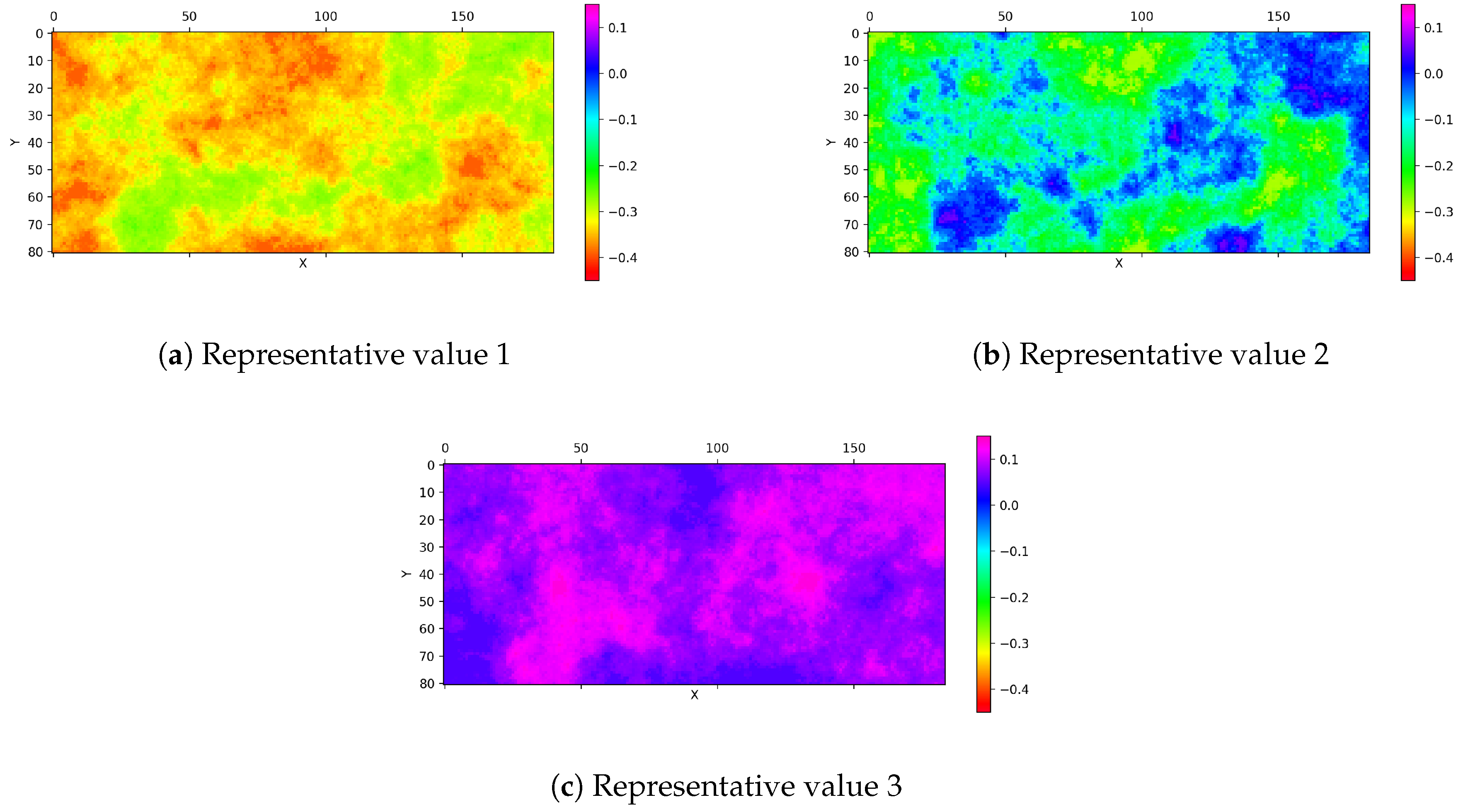
The representative values and the corresponding weights were thereafter used to scale the three error fields, as can be seen in Equation (5).
where is the SGS-produced random error field of the uncertain variable, i. Figure 2 shows the realizations of the random error field, , scaled by the representative values, ; their weights, ; and the standard deviation of the uncertain variable, . It is important that the range of values in three scaled random error fields is similar to that of the original random error field.
The simulation was run three times with the corresponding error fields. The statistical moments of the output variable were computed with Equation (4) as the weighted sum of the simulation results at the locations of the representative values to the power of the order of the statistical moment.
2.4. Workflow
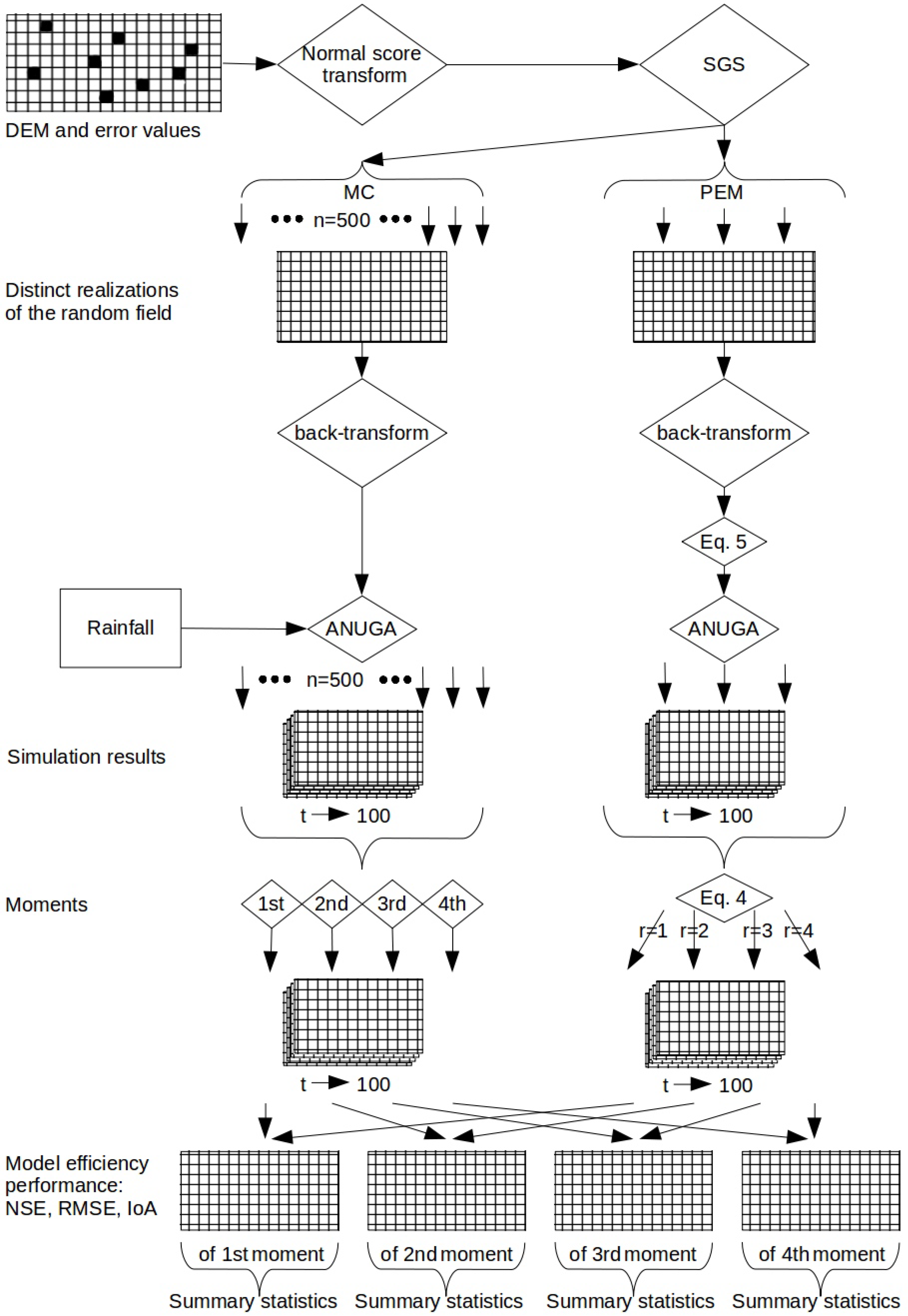
The Figure 3 illustrates the workflow of this study. The point of departure is the DEM and elevation of ground control locations. Both data sets combined result in error values. The error values need to be normalized because SGS requires that the input variable has a normal distribution. SGS generates 500 error fields for MC and three for PEM. The error values are back-transformed to the original distribution. Equation (5) scales the error fields for PEM. The error fields modify the DEM. The modified DEMs are supplied to ANUGA with the purpose to run an inundation scenario with a rainfall operator. The outputs are 500 raster time series data sets for MC and three for PEM. In the case of MC, the 500 raster time series data sets are reduced to four data sets, one for each statistical moment. In the case of PEM, Equation (4) estimates the raster time series data of the moments. The model efficiency performance measures finally compare the raster time series of each moment estimated by both methods. For each model efficiency performance measure, the results are one raster data set for each moment where each grid cell contains a model efficiency value. Each raster data set is subsequently summarized by mean, median, standard deviation, range and skew. The flowchart only displays the model efficiency performance assessment for the reason of readability.
2.5. Case Study
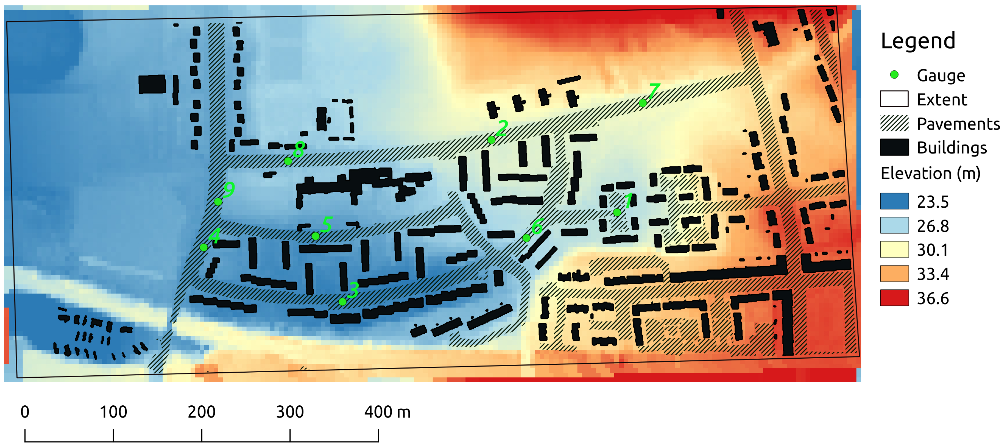
The location of the case study is Cockenzie Street and its surroundings in the city of Glasgow, UK. The data set was provided by the UK Environment Agency following their benchmark test No. 8 of two-dimensional hydraulic packages [41]. The data set contains the DEM, the geometry of buildings and roads, the Manning friction coefficients of paved and unpaved surfaces, the extent of the simulation domain, the location of the nine water level gauges and a rainfall curve. The study area is visualized in Figure 4. The DEM covers an area of approximately 0.4 km by 0.96 km. The original resolution of the DEM (0.5 m) was reduced to 5 m because of computational limitations. The range of the ground elevation is 21 m to 37 m. There are over 14.000 grid cells in the domain.
There are only two land cover categories with Manning friction coefficients: pavements (0.02) and unpaved surfaces (0.05). The simulation time was 1000 s with a 10-second time-step. The initial condition was a dry bed. The rainfall began after 1 min and lasted for 3 min with an intensity of 400 mm/h.
3. Results and Discussion
The model comparison below follows the recommendations in Bennett et al. [46] and Biondi et al. [47]. The times series at the nine gauge locations indicated in Figure 4 were visually compared. The similarities and differences of the spatial extents of the maximal inundations are then briefly assessed. The evaluation is completed by using the following model efficiency performance measures [47] on all time series over the whole spatial domain: Nash-Sutcliffe Model Efficiency (NSE), Root Mean Square Error (RMSE) and Index of Agreement (IoA). The statistical moments of MC should correspondingly be considered as “ground truth”, i.e., akin to observed data. We focus on the first and second statistical moments because of their more important relationship with real-world applications, but also consider the third and fourth moments because they permit the fitting of a probability distribution to the output variable.
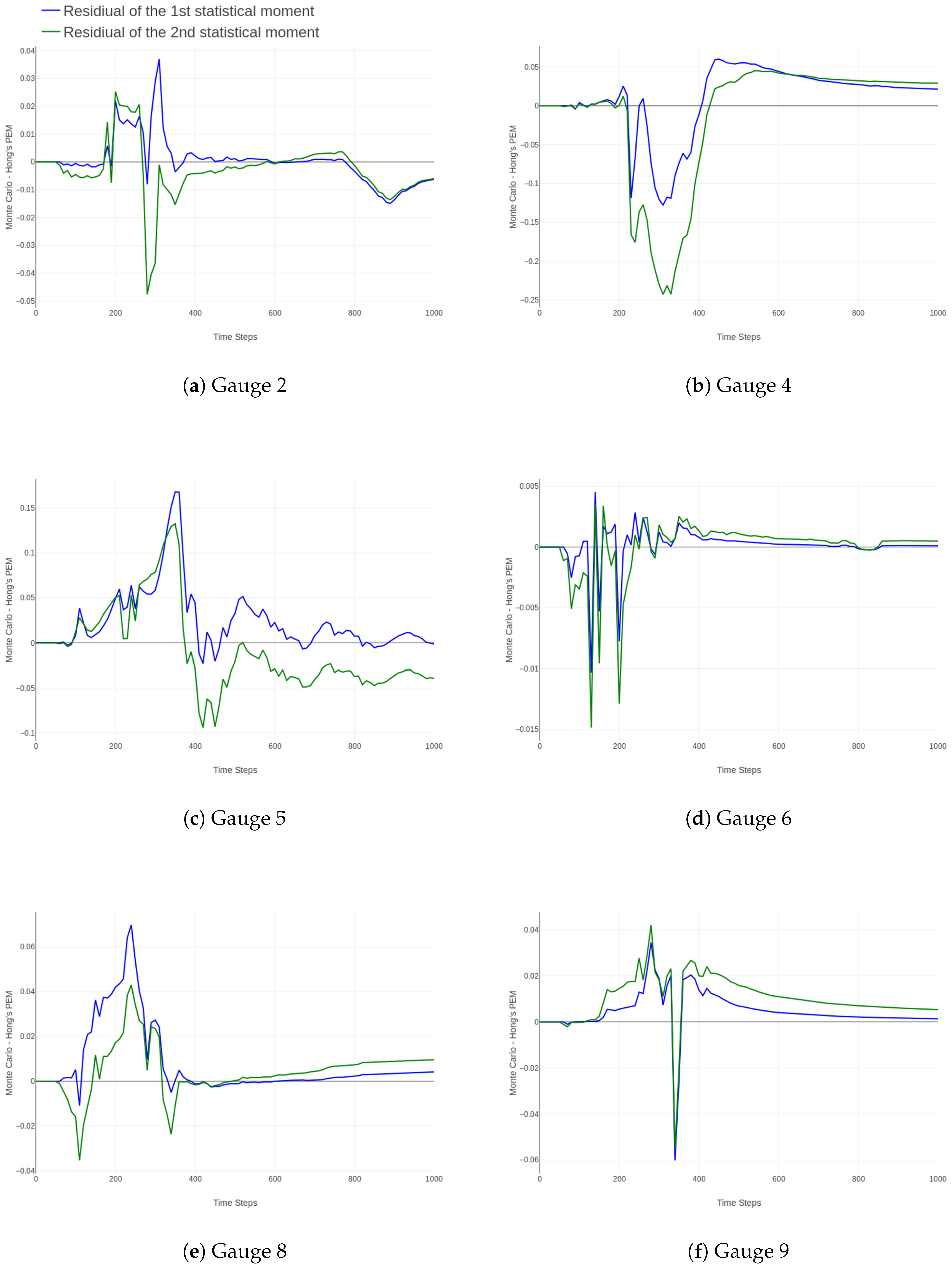
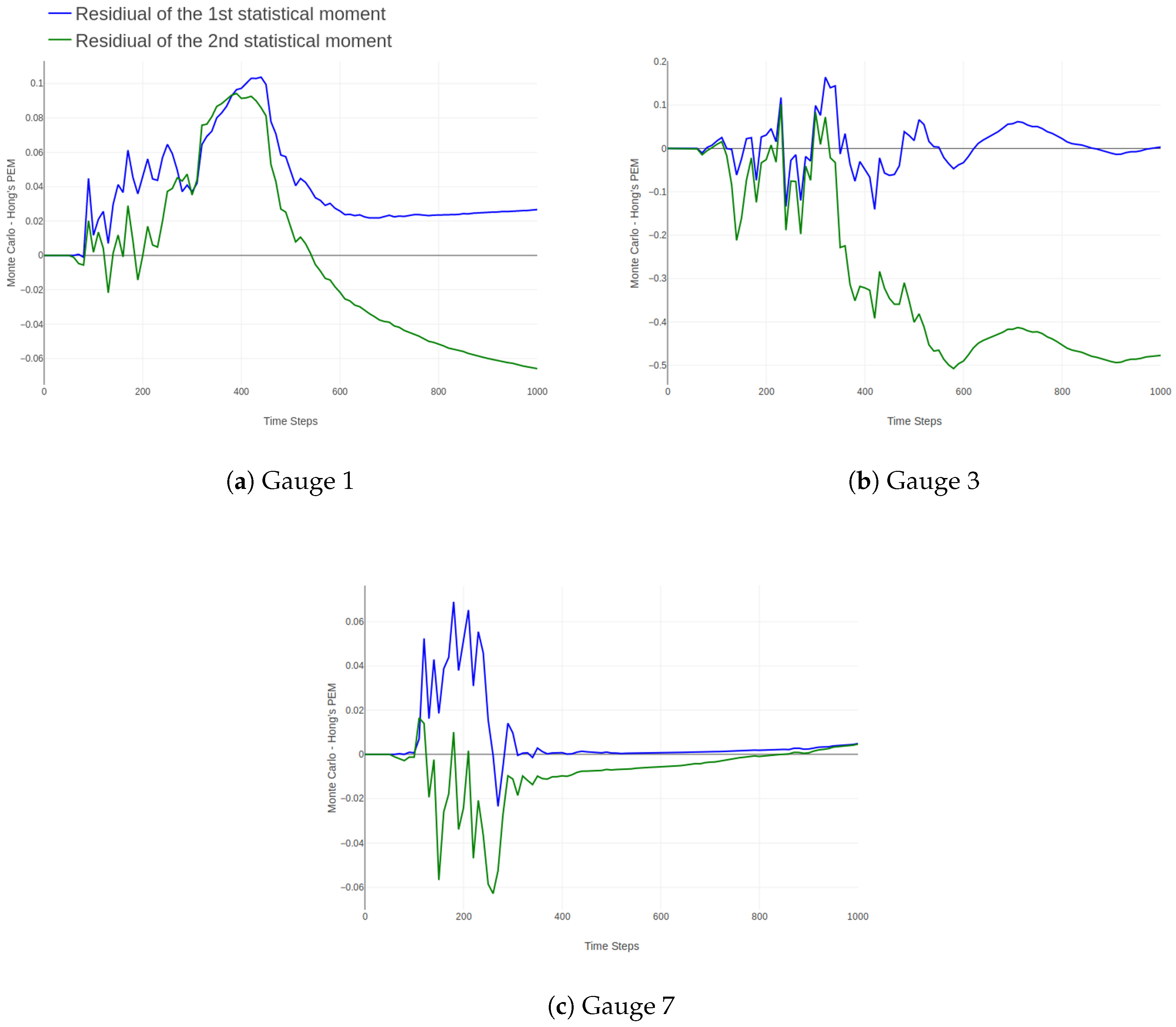
A comparison of the water depth values is shown using residual plots in Figure 5 and Figure 6. The residual plots show the differences and similarities over time. Figure 6 groups the time series with noteworthy behavior. During rainfall (from time-step 61 to 240), PEM mostly underestimates the first and second moment, except for at gauges 4 and 6 where it overestimates both moments. Gauge 7 is particular as PEM underestimates the first moment here but then overestimates the second moment. PEM also appears to be less sensitive during the more dynamic period, i.e., when mass (rainfall) is added to the system. Therefore, the residuals are much higher during these periods. After the rainfall had stopped, the output from MC and PEM converged at most gauges, except at gauges 1 and 3. PEM continued to slightly underestimate the first moment at most gauge locations while also overestimating the second moment at many gauge locations. Concerning the first moment, there is a bias towards MC, except at gauge 4. The plots show a bias of the second moment towards PEM, which is especially visible for gauge 3. The estimations of the second moment by PEM are also marked by outliers, especially for gauges 2, 6, 7 and 9. However, it is very sensitive to the multitude of paths runoff can take when slightly changing elevation. This is especially the case for the gauges grouped in Figure 6.
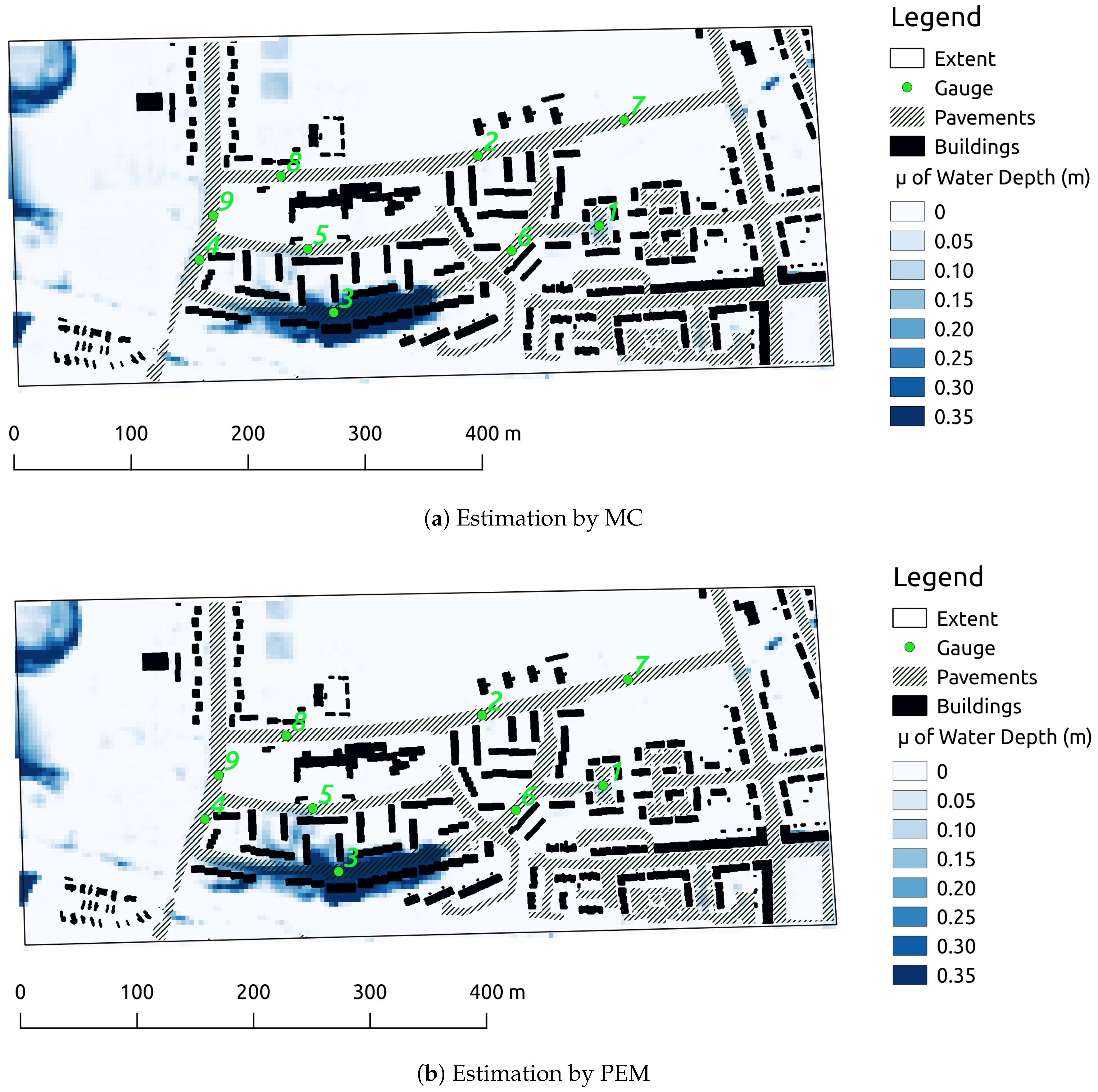
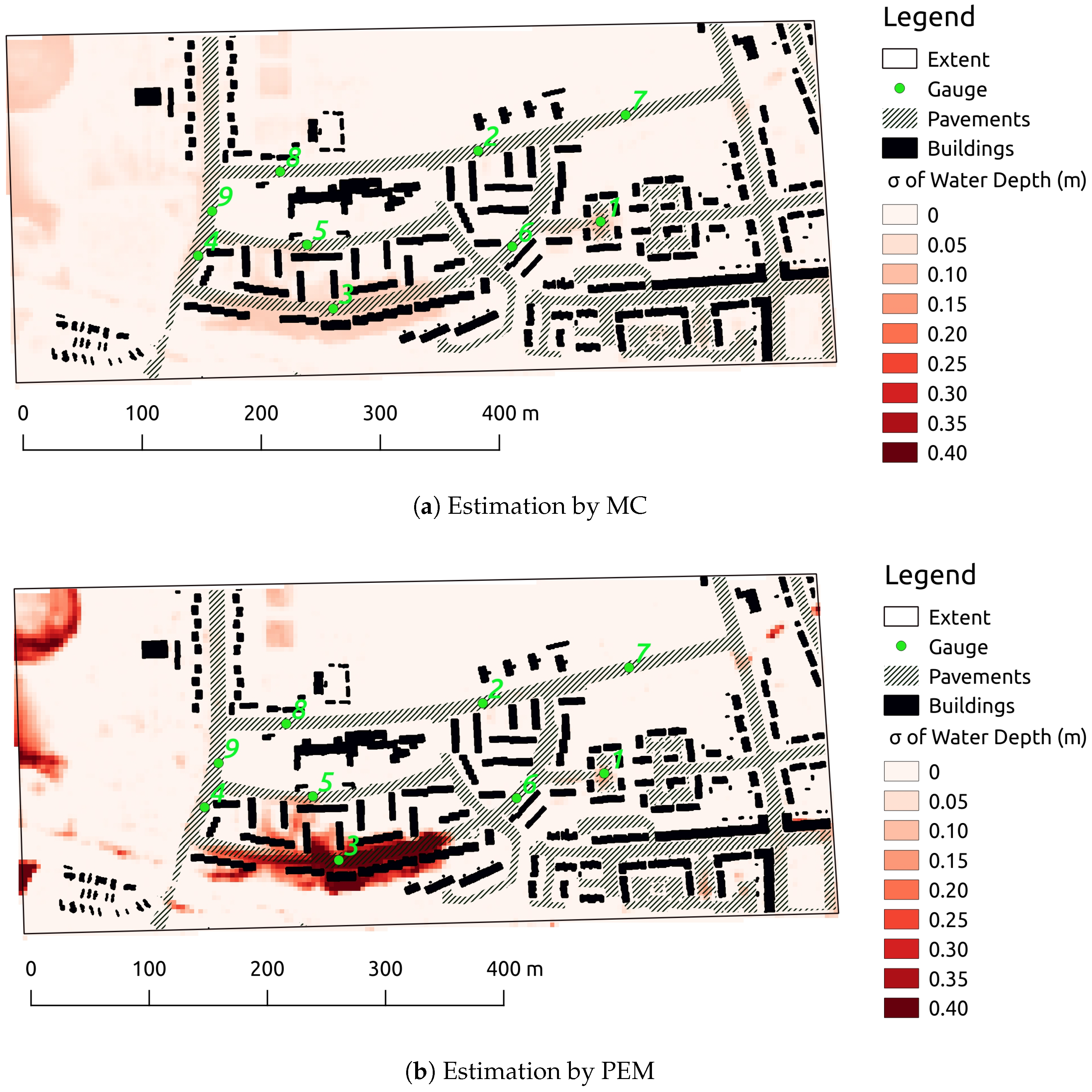
The spatial extent of the first two moments of the maximal flood inundation are compared in both Figure 7 and Figure 8 because peak water depth is important for practical purposes. The mean estimations by MC and PEM in Figure 7 depict a very similar spatial structure and magnitude. Figure 8 confirms the previous statements about the second moment. Despite similar spatial structures, the second moment is systematically overestimated by PEM. This observation is useful as it seems that PEM sets the upper limit for the second moment.
Table 1 summarizes the model efficiency performance measures for all time series of the estimated statistical moments. The model efficiency performance measures consequently compare the similarity between the results of MC and PEM. The empirical distributions of the performance measures are described by mean, median, standard deviation, range and skew. The column characterizes the means of the Nash–Sutcliffe efficiency between MC and PEM of every estimated moment. The other columns follow the same logic. The NSE in Table 1 is the most commonly employed performance measure in hydrology. It ranges from 1 to negative infinity, where 1 indicates a perfect match. The RMSE in Table 1 ranges from 0 to positive infinity, where 0 indicates a perfect match. The NSE and RMSE suffer potential bias when comparing models with offsets [46], perhaps because of the usage of the square root. To complement the evaluation, the IoA in Table 1 was also calculated. The advantage of using the IoA is that it uses absolute differences, and thus might better avoid bias. It ranges from 0 to 1, where 1 indicates a perfect match. The mean values for the performance measures for the first and second moments show a good match. The situation is further improved when regarding the median owing to the impact on the mean values of far outliers, as indicated by the range and skew values. The outliers also prevent the performance measures being summarized in a box plot. Estimations of the second moment by PEM yielded more under-outliers, as is clearly observed when comparing the negative mean of the NSE with the median. The third and fourth moments perform less well. The reasons for this appear to be more systematic because range and skew indicate that outliers are less of a problem than for the first and second moments. Interestingly, the NSE and IoA suggest that the estimations of the fourth moment match the observations better than those of the third moment, but RMSE suggests the opposite. The decreasing performance of the PEM estimations with the order of moments might have been caused by the usage of the square function in the calculation of the moments in Equation (4).
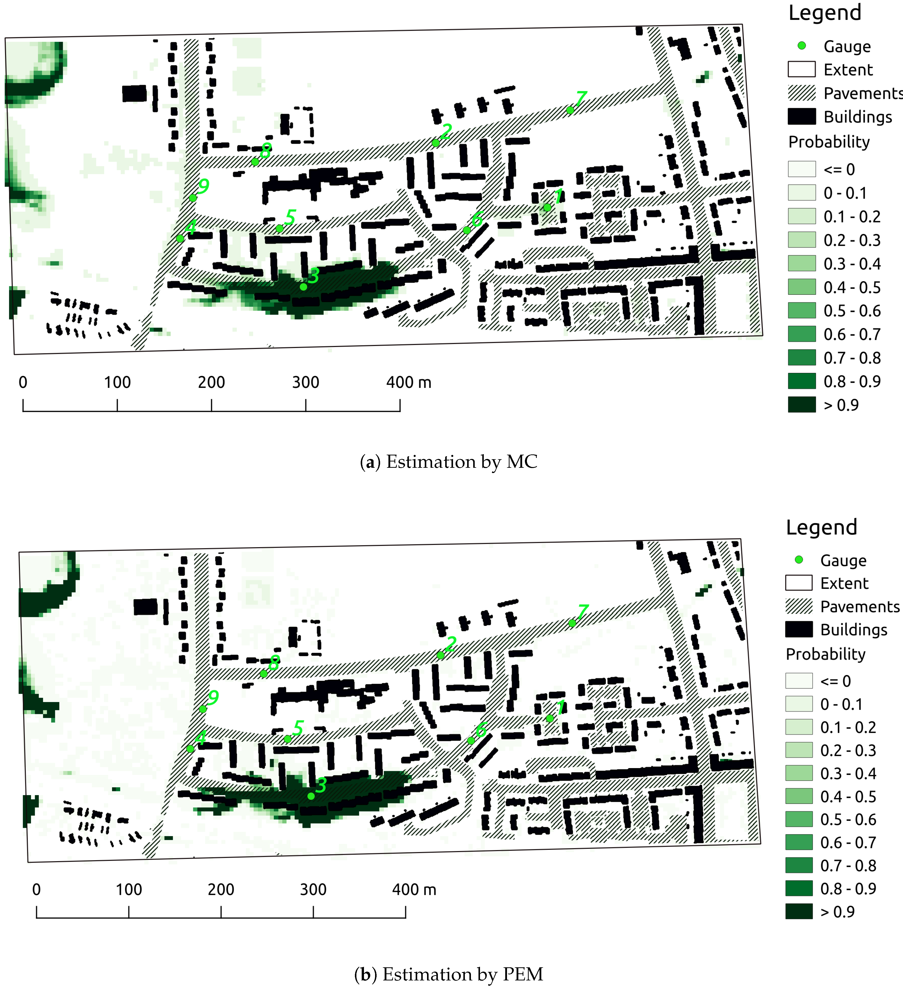
The end-product of this study is the probabilistic inundation map. The Gram-Charlier expansion, which was implemented using the R package PDQutils [48], was used to fit the statistical moments to a probability distribution based on a normal distribution. Figure 9 displays the probability of a maximal inundation over 0.2 m. Despite the differences of the higher moments between MC and PEM, PEM predicts a similar risk of inundation of over 0.2 m in terms of probability values and spatial extent.
4. Conclusions
This study demonstrated that PEMs are capable of approximating the uncertainty of an output in spatiotemporal models. Using PEMs instead of the more commonly used MC simulations yields considerable savings of computational resources. Instead of 500 simulation runs, each lasting 11 min for the data used in this study, only 3 simulation runs were required for the PEM approach. This decrease in computational resource requirement is especially important for spatiotemporal models because of the amount of data and the complexity involved. Methodological advances like this are key to development because challenges arising from the use of Big Data are unlikely to be overcome by increases in computational power alone, despite its continually falling cost.
Uncertainty analysis is important to mitigate the impact of an overreliance by practitioners on deceptive deterministic solutions that arise because fundamental natural principles are less deterministic than we think and our continued lack of capacity to model phenomena in their totality. While MC simulations are computationally too demanding to be widely adopted outside of the research community, PEMs’ ability to decrease computational costs could facilitate the uptake of uncertainty analysis in various fields. For example, hydrologists could combine water pollution models and PEMs to assess the risk of exceeding the legislated values (such as the U.S. EPA’s Total Maximum Daily Loads). In a similar fashion, PEMs could help to determine the risk of exceeding health-related air pollution thresholds. Concerning flooding, flood-control authorities and insurance companies could better evaluate the potential risks for critical infrastructure and for insured objects, respectively.
Future studies should investigate different implementations of PEMs for spatiotemporal models and how to accommodate multivariate cases, where spatial cross-correlation is of tremendous importance. Current visualization techniques need to be improved to exploit the full potential of the information furnished by uncertainty analysis.
Author Contributions
Conceptualization, M.I.; methodology, M.I.; software, M.I.; validation, M.I.; formal analysis, M.I.; investigation, M.I.; resources, M.I.; data curation, M.I.; writing—original draft preparation, M.I.; writing—review and editing, M.I.; visualization, M.I.; supervision, F.-J.C.; project administration, F.-J.C.; funding acquisition, F.-J.C. All authors have read and agreed to the published version of the manuscript.
Funding
This research and the APC was funded by the Ministry of Science and Technology, Taiwan (Grant number: 107-2621-M-002-004-MY3).
Acknowledgments
We are grateful to the UK Environment Agency for providing data. We also wish to thank Sam Pickard, Rainer Wunderlich, Bryon Flowers, Hangyeh Lin and Pierre-Alexandre Château for their constructive comments on previous versions of this article. The authors would like to thank the Editors and anonymous Reviewers for their constructive comments that are greatly contributive to the revision of the manuscript.
Conflicts of Interest
The authors declare no conflict of interest. The funders had no role in the design of the study; in the collection, analyses, or interpretation of data; in the writing of the manuscript, or in the decision to publish the results.
References
- Di Baldassarre, G.; Schumann, G.; Bates, P.D.; Freer, J.E.; Beven, K.J. Flood-plain mapping: A critical discussion of deterministic and probabilistic approaches. Hydrol. Sci. J. 2010, 55, 364–376. [Google Scholar] [CrossRef]
- Daniell, J.; Wenzel, F.; McLennan, A.; Daniell, K.; Kunz-Plapp, T.; Khazai, B.; Schaefer, A.; Kunz, M.; Girard, T. The global role of natural disaster fatalities in decision-making: statistics, trends and analysis from 116 years of disaster data compared to fatality rates from other causes. In Proceedings of the EGU General Assembly 2016 Conference, Vienna, Austria, 17–22 April 2016; Volume 18, p. 2021. [Google Scholar]
- Bubeck, P.; Kreibich, H.; Penning-Rowsell, E.C.; Botzen, W.; De Moel, H.; Klijn, F. Explaining differences in flood management approaches in Europe and in the USA–a comparative analysis. J. Flood Risk Manag. 2017, 10, 436–445. [Google Scholar] [CrossRef]
- Almeida, G.A.; Bates, P.; Freer, J.E.; Souvignet, M. Improving the stability of a simple formulation of the shallow water equations for 2-D flood modeling. Water Resour. Res. 2012, 48. [Google Scholar] [CrossRef]
- Bates, P.D. Integrating remote sensing data with flood inundation models: How far have we got? Hydrol. Process. 2012, 26, 2515–2521. [Google Scholar] [CrossRef]
- Hapuarachchi, H.A.P.; Wang, Q.J.; Pagano, T.C. A review of advances in flash flood forecasting. Hydrol. Process. 2011, 25, 2771–2784. [Google Scholar] [CrossRef]
- Merkuryeva, G.; Merkuryev, Y.; Sokolov, B.V.; Potryasaev, S.; Zelentsov, V.A.; Lektauers, A. Advanced river flood monitoring, modelling and forecasting. J. Comput. Sci. 2015, 10, 77–85. [Google Scholar] [CrossRef]
- Neal, J.; Villanueva, I.; Wright, N.; Willis, T.; Fewtrell, T.; Bates, P. How much physical complexity is needed to model flood inundation? Hydrol. Process. 2012, 26, 2264–2282. [Google Scholar] [CrossRef] [Green Version]
- Teng, J.; Jakeman, A.J.; Vaze, J.; Croke, B.F.; Dutta, D.; Kim, S. Flood inundation modelling: A review of methods, recent advances and uncertainty analysis. Environ. Model. Softw. 2017, 90, 201–216. [Google Scholar] [CrossRef]
- Stephens, E.M.; Bates, P.; Freer, J.; Mason, D. The impact of uncertainty in satellite data on the assessment of flood inundation models. J. Hydrol. 2012, 414, 162–173. [Google Scholar] [CrossRef] [Green Version]
- Wang, S.J.; Hsu, K.C. Dynamic interactions of groundwater flow and soil deformation in randomly heterogeneous porous media. J. Hydrol. 2013, 499, 50–60. [Google Scholar] [CrossRef]
- Chang, C.H.; Tung, Y.K.; Yang, J.C. Monte Carlo simulation for correlated variables with marginal distributions. J. Hydraul. Eng. 1994, 120, 313–331. [Google Scholar] [CrossRef]
- Graham, W.; McLaughlin, D. Stochastic analysis of nonstationary subsurface solute transport: 2. Conditional moments. Water Resour. Res. 1989, 25, 2331–2355. [Google Scholar] [CrossRef]
- Li, S.G.; McLaughlin, D. A nonstationary spectral method for solving stochastic groundwater problems: Unconditional analysis. Water Resour. Res. 1991, 27, 1589–1605. [Google Scholar] [CrossRef]
- Gires, A.; Onof, C.; Maksimovic, C.; Schertzer, D.; Tchiguirinskaia, I.; Simoes, N. Quantifying the impact of small scale unmeasured rainfall variability on urban runoff through multifractal downscaling: A case study. J. Hydrol. 2012, 442, 117–128. [Google Scholar] [CrossRef] [Green Version]
- Tung, Y.K. Mellin transform applied to uncertainty analysis in hydrology/hydraulics. J. Hydraul. Eng. 1990, 116, 659–674. [Google Scholar] [CrossRef]
- Che-Hao, C.; Yeou-Koung, T.; Jinn-Chuang, Y. Evaluation of probability point estimate methods. Appl. Math. Model. 1995, 19, 95–105. [Google Scholar] [CrossRef]
- Franceschini, S.; Tsai, C.; Marani, M. Point estimate methods based on Taylor Series Expansion—The perturbance moments method—A more coherent derivation of the second order statistical moment. Appl. Math. Model. 2012, 36, 5445–5454. [Google Scholar] [CrossRef]
- Harr, M.E. Probabilistic estimates for multivariate analyses. Appl. Math. Model. 1989, 13, 313–318. [Google Scholar] [CrossRef]
- Hong, H.P. An efficient point estimate method for probabilistic analysis. Reliab. Eng. Syst. Saf. 1998, 59, 261–267. [Google Scholar] [CrossRef]
- Rosenblueth, E. Point estimates for probability moments. Proc. Natl. Acad. Sci. USA 1975, 72, 3812–3814. [Google Scholar] [CrossRef] [Green Version]
- Rosenblueth, E. Two-point estimates in probabilities. Appl. Math. Model. 1981, 5, 329–335. [Google Scholar] [CrossRef]
- Christakos, G. Random Field Models in Earth Sciences; Courier Corporation: North Chelmsford, MA, USA, 2012. [Google Scholar]
- Aerts, J.C.J.H.; Goodchild, M.F.; Heuvelink, G.B.M. Accounting for Spatial Uncertainty in Optimization with Spatial Decision Support Systems. Trans. GIS 2003, 7, 211–230. [Google Scholar] [CrossRef] [Green Version]
- Ehlers, L.; Refsgaard, J.C.; Sonnenborg, T.O.; He, X.; Jensen, K.H. Using sequential Gaussian simulation to quantify uncertainties in interpolated gauge based precipitation. In Proceedings of the EGU General Assembly 2016 Conference, Vienna, Austria, 17–22 April 2016; Volume 18, p. 15751. [Google Scholar]
- Gonçalvès, J.; Vallet-Coulomb, C.; Petersen, J.; Hamelin, B.; Deschamps, P. Declining water budget in a deep regional aquifer assessed by geostatistical simulations of stable isotopes: Case study of the Saharan “Continental Intercalaire”. J. Hydrol. 2015, 531, 821–829. [Google Scholar] [CrossRef]
- Varouchakis, E.A.; Hristopulos, D.T. Dynamic Modelling of Aquifer Level Using Space-Time Kriging and Sequential Gaussian Simulation. In Proceedings of the EGU General Assembly 2016 Conference, Vienna, Austria, 17–22 April 2016; Volume 18, p. 11694. [Google Scholar]
- Shields, M.D.; Teferra, K.; Hapij, A.; Daddazio, R.P. Refined stratified sampling for efficient Monte Carlo based uncertainty quantification. Reliab. Eng. Syst. Saf. 2015, 142, 310–325. [Google Scholar] [CrossRef] [Green Version]
- Wu, K.; Li, J. A surrogate accelerated multicanonical Monte Carlo method for uncertainty quantification. J. Comput. Phys. 2016, 321, 1098–1109. [Google Scholar] [CrossRef] [Green Version]
- Gurdak, J.J.; Qi, S.L. Vulnerability of Recently Recharged Ground Water in the High Plains Aquifer to Nitrate Contamination; Technical Report; U. S. Geological Survey: Reston, VA, USA, 2006.
- Niemunis, A.; Wichtmann, T.; Petryna, Y.; Triantafyllidis, T. Stochastic modelling of settlements due to cyclic loading for soil-structure interaction. In Proceedings of the International Conference on Structural Damage and Lifetime Assessment, Rome, Italy, 17–18 February 2005; Volume 18. [Google Scholar]
- Tejchman, J.; Górski, J. Deterministic and statistical size effect during shearing of granular layer within a micro-polar hypoplasticity. Int. J. Numer. Anal. Methods Geomech. 2008, 32, 81–107. [Google Scholar] [CrossRef]
- Dodwell, T.J.; Ketelsen, C.; Scheichl, R.; Teckentrup, A.L. A hierarchical multilevel Markov chain Monte Carlo algorithm with applications to uncertainty quantification in subsurface flow. SIAM/ASA J. Uncertain. Quantif. 2015, 3, 1075–1108. [Google Scholar] [CrossRef] [Green Version]
- Moradkhani, H.; DeChant, C.M.; Sorooshian, S. Evolution of ensemble data assimilation for uncertainty quantification using the particle filter-Markov chain Monte Carlo method. Water Resour. Res. 2012, 48. [Google Scholar] [CrossRef]
- Vrugt, J.A.; Ter Braak, C.J.; Clark, M.P.; Hyman, J.M.; Robinson, B.A. Treatment of input uncertainty in hydrologic modeling: Doing hydrology backward with Markov chain Monte Carlo simulation. Water Resour. Res. 2008, 44. [Google Scholar] [CrossRef] [Green Version]
- Feinberg, J.; Langtangen, H.P. Chaospy: An open source tool for designing methods of uncertainty quantification. J. Comput. Sci. 2015, 11, 46–57. [Google Scholar] [CrossRef] [Green Version]
- Suchomel, R.; Mašı, D. Comparison of different probabilistic methods for predicting stability of a slope in spatially variable c-phi soil. Comput. Geotech. 2010, 37, 132–140. [Google Scholar] [CrossRef]
- Nielsen, O.; Roberts, S.; Gray, D.; McPherson, A.; Hitchman, A. Hydrodynamic modelling of coastal inundation. In Proceedings of the MODSIM 2005 International Congress on Modelling and Simulation, Melbourne, Austrilia, 12–15 December 2005; pp. 518–523. [Google Scholar]
- Roberts, S.; Nielsen, O.; Gray, D.; Sexton, J. ANUGA User Manual; Geoscience Australia and Australian National University: Canberra, Austrilia, 2010. [Google Scholar]
- Mungkasi, S.; Roberts, S. Validation of ANUGA hydraulic model using exact solutions to shallow water wave problems. J. Phys. Conf. Ser. 2013, 423, 012029. [Google Scholar] [CrossRef] [Green Version]
- Néelz, S.; Pender, G. Benchmarking the Latest Generation of 2D Hydraulic Modelling Packages; Technical Report SC120002; UK Environment Agency: Rotherham, UK, 2013.
- Fan, Y.; Huang, W.; Huang, G.; Huang, K.; Zhou, X. A PCM-based stochastic hydrological model for uncertainty quantification in watershed systems. Stoch. Environ. Res. Risk Assess. 2015, 29, 915–927. [Google Scholar] [CrossRef]
- Miller, K.; Berg, S.; Davison, J.; Sudicky, E.; Forsyth, P. Efficient uncertainty quantification in fully-integrated surface and subsurface hydrologic simulations. Adv. Water Resour. 2018, 111, 381–394. [Google Scholar] [CrossRef]
- Deutsch Clayton, V.; Journel André, G. GSLIB Geostatistical Software Library and User’s Guide; Oxford University Press: Oxford, UK, 1998. [Google Scholar]
- Savichev, V.; Bezrukov, A.; Muharlyamov, A.; Barskiy, K.; Rustam, S. High Performance Geostatistics Library. 2010. Available online: http://hpgl.github.io/hpgl/index.html (accessed on 13 October 2017).
- Bennett, N.D.; Croke, B.F.; Guariso, G.; Guillaume, J.H.; Hamilton, S.H.; Jakeman, A.J.; Marsili-Libelli, S.; Newham, L.T.; Norton, J.P.; Perrin, C. Characterising performance of environmental models. Environ. Model. Softw. 2013, 40, 1–20. [Google Scholar] [CrossRef]
- Biondi, D.; Freni, G.; Iacobellis, V.; Mascaro, G.; Montanari, A. Validation of hydrological models: Conceptual basis, methodological approaches and a proposal for a code of practice. Phys. Chem. Earth Parts A/B/C 2012, 42, 70–76. [Google Scholar] [CrossRef]
- Pav, S. PDQ Functions via Gram Charlier, Edgeworth, and Cornish Fisher Approximations. 2017. Available online: https://cran.r-project.org/web/packages/PDQutils/index.html (accessed on 13 October 2017).
Figure 1.
Histogram showing the elevation error and the location of the representative values (red): mean = −0.12, standard deviation = 0.14.
Figure 1.
Histogram showing the elevation error and the location of the representative values (red): mean = −0.12, standard deviation = 0.14.

Figure 2.
The random error field produced by SGS and scaled according to Equation (5) for three representative values.
Figure 2.
The random error field produced by SGS and scaled according to Equation (5) for three representative values.

Figure 3.
Workflow of the study.

Figure 4.
Digital Elevation Map with land cover of the area around Cockenzie Street in Glasgow, UK.

Figure 5.
Residual plots showing similarities and differences between predictions made by MC simulation and PEM.
Figure 5.
Residual plots showing similarities and differences between predictions made by MC simulation and PEM.

Figure 6.
Residual plots showing similarities and differences between predictions made by MC simulation and PEM for gauges with noteworthy behaviour.
Figure 6.
Residual plots showing similarities and differences between predictions made by MC simulation and PEM for gauges with noteworthy behaviour.

Figure 7.
Map of the 1st statistical moment of maximal water depth.

Figure 8.
Map of the 2nd statistical moment of maximal water depth.

Figure 9.
Probabilistic inundation maps showing the probability of inundation over 0.2 m.


Table 1.
Summary statistics of model efficiency performance for all time series of the estimated statistical moments at each grid cell.
Table 1.
Summary statistics of model efficiency performance for all time series of the estimated statistical moments at each grid cell.
| 1st Moment | 0.73 | 0.99 | 2.35 | 141.49 | −34.87 |
| 2nd Moment | −1.95 | 0.96 | 38.10 | 2008.66 | −35.86 |
| 3rd Moment | −0.78 | −0.25 | 1.81 | 12.61 | −1.72 |
| 4th Moment | 0.07 | −0.32 | 0.96 | 10.92 | −1.74 |
| 1st Moment | 0.0074 | 0.0007 | 0.0164 | 0.1775 | 3.6896 |
| 2nd Moment | 0.0179 | 0.0014 | 0.054 | 0.9263 | 6.1075 |
| 3rd Moment | 5.092 | 3.6726 | 4.101 | 20.4579 | 1.0632 |
| 4th Moment | 74.6667 | 33.7397 | 85.76 | 443.706 | 1.7032 |
| 1st Moment | 0.96 | 0.99 | 0.09 | 0.96 | −5.28 |
| 2nd Moment | 0.88 | 0.99 | 0.18 | 0.99 | −2.22 |
| 3rd Moment | 0.55 | 0.64 | 0.35 | 0.99 | −0.23 |
| 4th Moment | 0.62 | 0.81 | 0.36 | 0.99 | −0.51 |
© 2020 by the authors. Licensee MDPI, Basel, Switzerland. This article is an open access article distributed under the terms and conditions of the Creative Commons Attribution (CC BY) license (http://creativecommons.org/licenses/by/4.0/).
Share and Cite
MDPI and ACS Style
Issermann, M.; Chang, F.-J. Uncertainty Analysis of Spatiotemporal Models with Point Estimate Methods (PEMs)—The Case of the ANUGA Hydrodynamic Model. Water 2020, 12, 229. https://doi.org/10.3390/w12010229
AMA Style
Issermann M, Chang F-J. Uncertainty Analysis of Spatiotemporal Models with Point Estimate Methods (PEMs)—The Case of the ANUGA Hydrodynamic Model. Water. 2020; 12(1):229. https://doi.org/10.3390/w12010229
Chicago/Turabian StyleIssermann, Maikel, and Fi-John Chang. 2020. "Uncertainty Analysis of Spatiotemporal Models with Point Estimate Methods (PEMs)—The Case of the ANUGA Hydrodynamic Model" Water 12, no. 1: 229. https://doi.org/10.3390/w12010229
Note that from the first issue of 2016, this journal uses article numbers instead of page numbers. See further details here.