Identification of Parameters of Evaporation Equations Using an Optimization Technique Based on Pan Evaporation

Abstract

Countries in arid regions are presently facing challenges in managing their limited water resources. Assessing the evaporation losses from various sources of water is a daunting task that is inevitable for the sustainability of water resource management schemes in these regions. Although several techniques are available for simulating evaporation rates, identifying the parameters of various evaporation equations still needs to be further investigated. The main goal of this research was to develop a framework for determining the parameters influencing the evaporation rate of evaporation pans. Four different equations, including those of Hamon, Penman, Jensen–Haise, and Makkink, were chosen to estimate evaporation from the evaporation pans installed in the Qassim Region of Saudi Arabia. The parameters of these four equations were identified by a state-of-the-art optimization technique, known as the general reduced gradient (GRG). Three types of objective functions used for optimization were tested. Forty-year monitoring records for pan evaporation, temperature, relative humidity, and sunshine hours were collected from the Municipality of Buraydah Al Qassim, for the period of 1976 to 2016. These data were mainly manually recorded at a weather station situated in the Buraydah city. Preliminary data analysis was performed using the Mann–Kendall and Sen’s slope tests to study the trends. The first 20-year (1976–1995) data were used for calibrating the equations by employing an optimization technique and the remaining data were used for validation purposes. Four new equations were finally developed and their performance, along with the performance of the four original equations, was evaluated using the Nash and Sutcliffe Efficiency (NSE) and the Mean Biased Error (MBE). The study revealed that among the original equations, the Penman equation performed better than the other three equations. Additionally, among the new equations, the Hamon method performed better than the remaining three equations.

1. Introduction

Environmental, industrial, and climatic changes are affecting the hydrological cycle of different regions, worldwide. Due to such changes, the shortage of water resources has become a serious threat to arid environmental areas, such as the Gulf region. Evaporation loss is an important component of the hydrological cycle and precise estimation of the rate of evaporation from various sources of water plays an important role in the planning, design, and operation of natural water resources, particularly in arid regions. Therefore, the evaporation loss should be given appropriate attention while dealing with water/energy budgets and climate change impacts [1,2,3].

Evaporation rate estimation in irrigated areas and other water bodies is highly complex due to the nonlinear behavior of various physical processes that affect vaporization. Several equations exist for calculating the evaporation rates of various water bodies and evaporation pans [2,4,5,6,7,8], and each one of them provides different results. Therefore, selecting the most appropriate equation for estimating evaporation rates remains a vital research topic [9,10,11,12,13]. The availability and accuracy of data is another issue to be addressed. For arid regions, it is of utmost importance to compare and evaluate the methods of estimating evaporation, in order to select the best evaporation equation for the future planning of limiting water resources. Inaccuracies in estimated evaporation will directly affect the design, operation, and maintenance of drainage facilities, irrigation schedules, and runoff estimations. As equations based on physical principles require a lot of data and most of the empirical equations are site-dependent, the empirical parameters of these equations must be determined with an acceptable degree of certainty [11,12,13]. Identification of the parameters of the evaporation equations requires the application of a suitable optimization technique. This aspect has not been frequently investigated in past studies.

There are many meteorological factors affecting the rate of evaporation, including (i) the temperature of the water and air, (ii) the difference in vapor pressure between water and air, (iii) the wind speed, and (iv) solar radiation [14,15]. The evaporation rate is also influenced by the surrounding air humidity. Humid air (moist air) has a comparatively smaller thirst for water vapor than drier air, while an absence of wind also decreases the evaporation rate. During non-windy days, water evaporating to the adjacent air remain close to the surface of the pond or reservoir and contribute to the local humidity. The evaporation rate diminishes when the moisture content of the adjacent air reaches the maximum limiting value. The existence of airflow removes the vapor of the air surrounding the water source, which reduces the humidity and thus increases the evaporation rate [14,16].

The evaporation process needs sufficient energy for the latent heat of vaporization. The main source of heat energy is solar radiation. [14,17,18,19].

Numerous methods exist for estimating evaporation from water surfaces [2,4,5,6,7,8,11,12,13,20]. These methods fall into four categories, namely, the (i) water budget, (ii) energy budget, (iii) method of mass transfer, and (iv) combined techniques. In energy budget and water budget techniques, the incoming and outgoing amounts are balanced. The equations obtained from this balance are solved by keeping the evaporation rate unknown [20,21]. The most useful methods for estimating evaporation calculate the evaporation rates by using meteorological records. The Penman equation [22] forms the basis of derivation for most of these methods. Details of many other research publications on assessing evaporation rates from the water surface or potential evapotranspiration (equivalent to evaporation) can be found in the literature [11,16,17,20,23]. These evaporation estimation methods can also be classified as direct techniques (eddy correlation techniques and large evaporation pan techniques) and indirect techniques (water balance techniques, aerodynamic techniques, heat balance techniques, etc.) [24]. Recent research has been done on the design and validation of evaporation pans by Collison [25]. According to him, pans that are installed in a way that represent the actual field conditions might produce accurate results, whereas the Class A Pan and other standard pans in use usually provide slightly inaccurate measured evaporation. Tanny et al. [26] and Chu et al. [27] conducted research related to the Class A evaporation pan and found that it is the least accurate method of measuring and estimating evaporation. All such limitations must be considered while dealing with evaporation estimates. It all depends upon the nature of the project one is dealing with. The estimation of evaporation losses for various components of water resource planning and management includes different aspects. For example, in case of runoff estimation from a catchment, the constants of evaporation equations and data required for the development of the equations might be different from those used for evaporation estimation, while dealing with irrigation scheduling or reservoir operations.

Table 1. Data requirements and review of publications regarding evaporation equations.

Reference	Data Required				Identified Parameters by Optimization
	Temperature	Humidity	Wind	Radiation
Yang and Roderick 2019 [2]	√	×	√	√	×
Stassen et al. 2019 [3]	√	×	√	×	×
Wang et al. 2019 [4]	√	√	√	×	×
Ahmadipour et al. 2019 [5]	√	√	√	×	×
Zolá et al. 2019 [6]	√	×	√	×	×
Al-Domany et al. 2018 [7]	√	×	√	×	×
Duan and Bastiaanssen 2017 [8]	√	×	√	√	×
Said and Hussein 2013 [10]	√	√	×	×	×
Hussein 2015 [12]	√	√	√	√	×
Patel and Majmundar 2016 [13]	√	×	×	√	×
Majidi et al. 2015 [20]	√	×	×	√	×
Morton 1971 [28]	√	√	×	×	×
Yao and Creed 2005 [29]	√	√	×	×	×
Winter et al. 1995 & 2003 [30,31]	√	√	×	√	×
Moazed et al. 2014 [32]	√	√	√	√	×
Paparrizos et al. 2014 [33]	√	√	√	√	×

summarizes the data needed and limitations of some of more recent studies.

The water loss per unit time from a standard container is often measured at weather stations. The most commonly used techniques for measuring evaporation rates are evaporation pans, which are inexpensive and simple to operate. The US Weather Bureau Class A pan is one of the best-known pans equipped with a level sensor. As the actual evaporation is less than the evaporation measured by pans, the pan coefficient defines the ratio of actual pond evaporation and measured pan evaporation rates [10,34].

Pan evaporation has been used in a number of research projects to choose the most appropriate evaporation equation in various parts of the world [35,36,37,38,39]. Ali et al. [40,41] found a strong agreement of the monthly average of Class A pan evaporation with the estimates of the Penman equation [42]. Tukimat et al. [43] compared a number of temperature- and radiation-based methods with the Penman–Monteith equation to estimate evaporation. According to them, the methods based on radiation simulated comparatively better results for evaporation and potential evapotranspiration. Pan evaporation has been compared with the estimated values of evaporation from eight empirical equations by Lee et al. [38]. They found comparatively better agreement between pan evaporation and estimates of the Penman–Monteith equation [44]. Muniandy et al. [39] compared the estimates of pan evaporation with the results of 26 empirical equations. According to them, the Penman equation provided comparatively better estimates of evaporation compared to other methods.

A summary of the literature review shows that the identification of parameters of evaporation equations using state-of-the-art optimization techniques has rarely been reported, whereas this aspect is of the utmost importance for developing robust evaporation equations for a specific region. Therefore, the main objectives of the present research were to (i) compare the results of some existing evaporation equations with actually measured pan evaporation data and choose the best one, (ii) determine the parameters of evaporation equations using state-of-the-art optimization methods, and (iii) compare the results of different developed evaporation equations with pan evaporation data. Extensive data were obtained from the Municipality of Buraydah, Qassim, Saudi Arabia, to achieve the above stated objectives and to evaluate the practicality of our approach for estimating more accurate evaporation losses from natural ponds in arid regions.

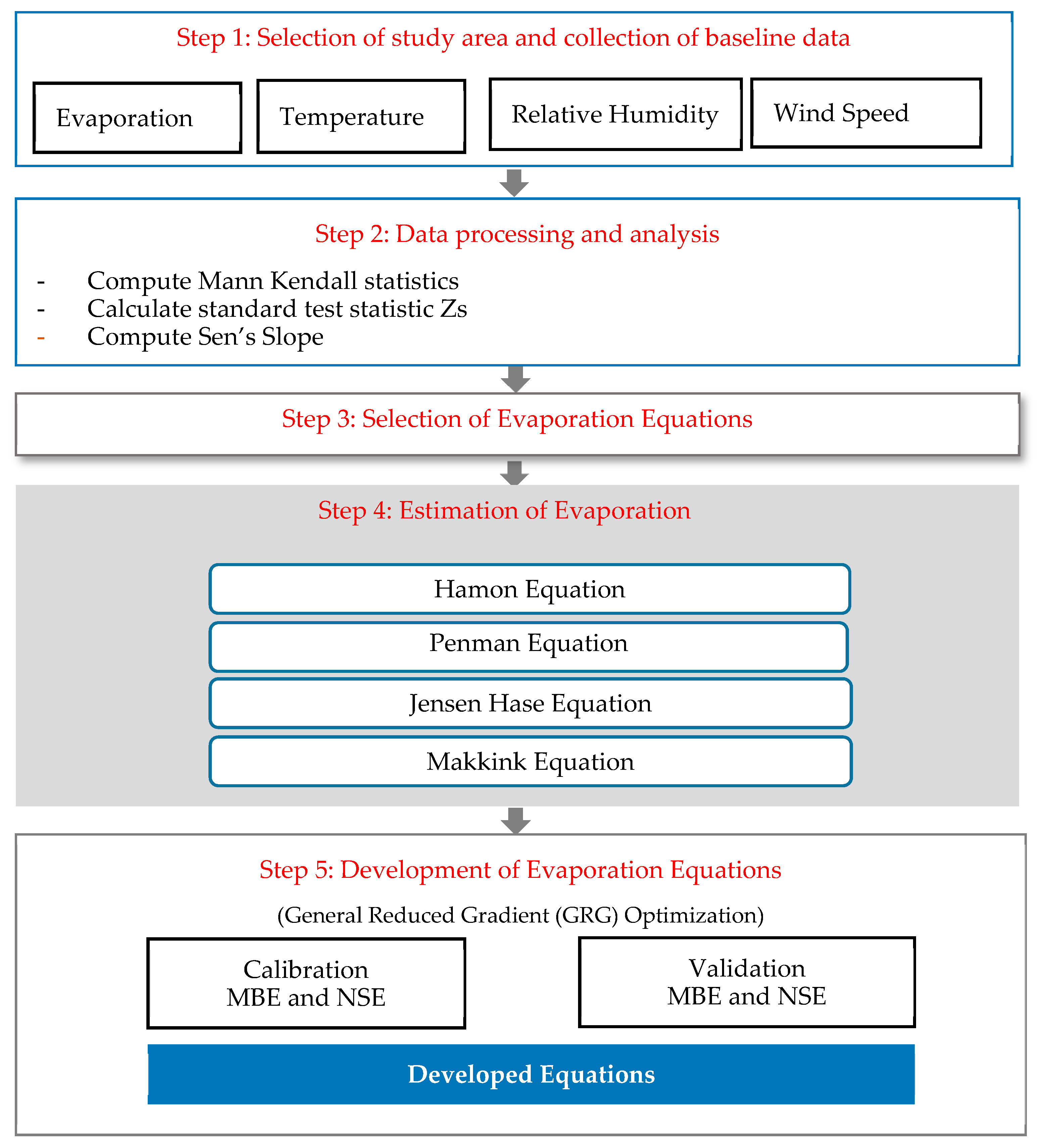
2. Materials and Methods

The framework for the methodology is given in Figure 1. The most difficult task in this research was to collect the extensive data required for the calibration, development, and validation of evaporation equations on the basis of pan evaporation. These data were collected from the Municipality of Buraydah, Qassim, Saudi Arabia, as mentioned above. A brief summary of evaporation and other meteorological data measurement is described below.

In the era of high technology, there are sophisticated methods available to directly measure lake evaporation [6]. However, either data from advanced techniques that use sensors to measure evaporation are not yet easily available in developing countries, or the available data are not sufficient for statistical analyses and the development of equations. Pan evaporation is considered a reasonably good indicator of the regional evaporation intensity that is usually used for estimations of lake evaporation and water resource planning and management [14]. Pan evaporation and meteorological variables, including solar radiation, sunshine duration, atmospheric pressure, vapor pressure, wind velocity, air temperature, and relative humidity, were used in a study on lake evaporation by Yan et al. [14]. A monthly pan evaporation dataset was used for monitoring and estimating important aspects of evaporation in various parts of the world [11,12,13,14].

2.1. Data Collection

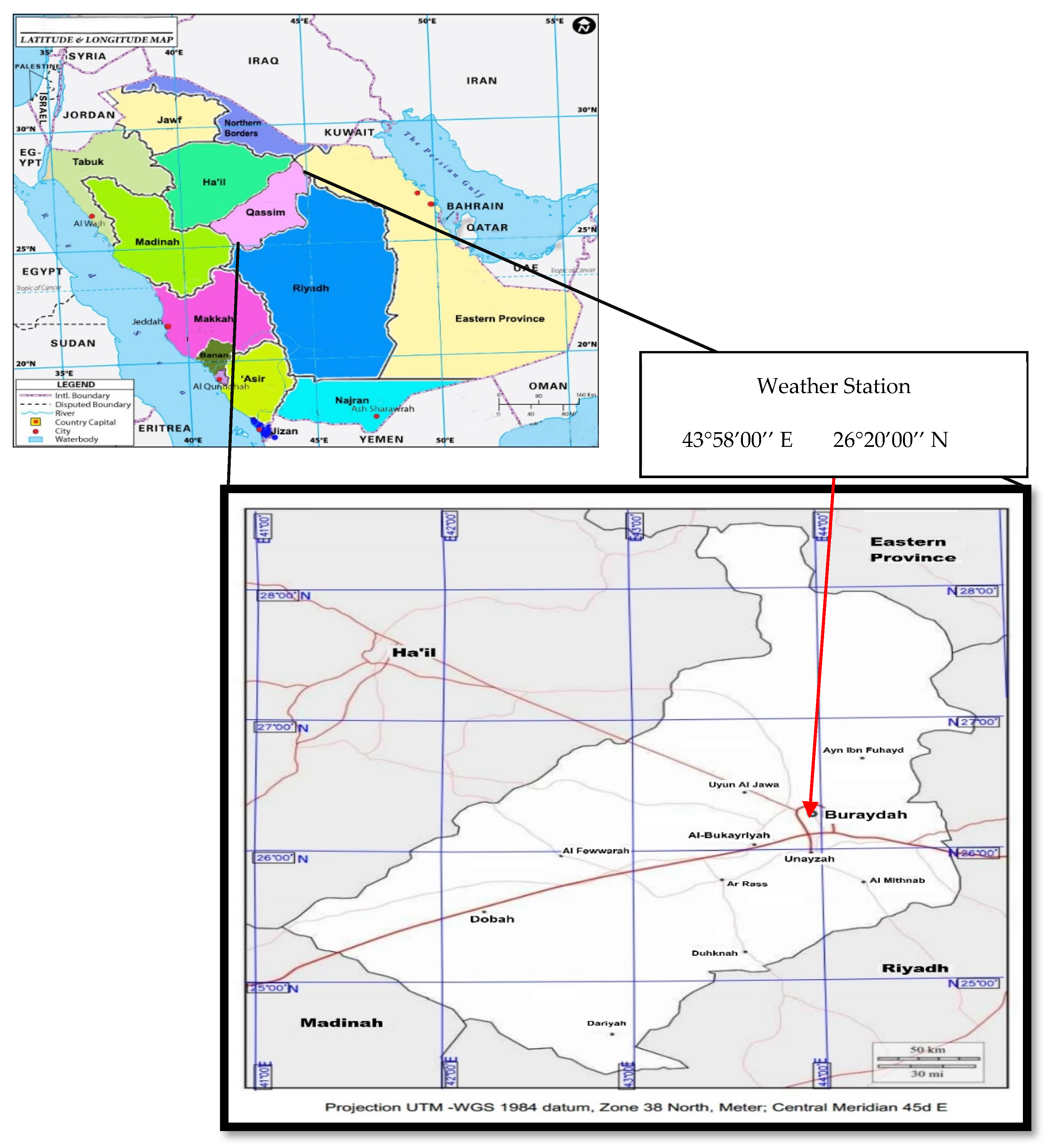
The records of evaporation and meteorological data, including relative humidity, temperature, wind speed, and sunshine hours, were collected from the Municipality of Buraydah Al Qassim. A manually operated pan was used for the collection of evaporation data. In this study, such data were selected so that the equations developed could be based on long-term data. The Class A pan had a height of 25.4 cm and a diameter of 120.7 cm. It was made of stainless steel and was installed on a wooden platform placed on the ground in a location away from obstacles, including trees and bushes, so that there was a natural airflow around the pan. Pan evaporation was measured on a daily basis in terms of the depth of water (mm) evaporated from the pan. However, to take into account the actual conditions of lakes, a pan coefficient was involved to convert the pan evaporation to lake evaporation. The pan coefficient used to convert pan evaporation into lake evaporation in this study was taken as 0.75, as provided by the authority from which the data were collected. According to the data-providing authority, the pan was changed only a few years ago but was also a Class A pan, so the results of pan evaporation could be considered consistent with previous records. The other meteorological data, including temperature, relative humidity, and wind speed, were measured by fully automated devices that have been connected by a computer for the last about five years. The remaining data were manually recorded. The fully computerized data were available for a short period. A thorough comparison of the two types of data was not performed. However, there was hardly any difference between the important values of temperature, like the average, maximum, and minimum temperature. The relative humidity was recorded by a psychrometer, temperature was measured by minimum and maximum thermometers, and wind speed was measured by an anemometer.

2.2. Study Area

The weather station was situated near the Buraydah City Center (Figure 2), which was used to measure the evaporation from pan along with other meteorological data. The first data scrutiny was conducted by visual inspection of the data, checking value by value. Abnormal values, like zero evaporation against a temperature range of 30 to 40 °C, were removed. Relative humidity values greater than 100% were also removed. The cells corresponding to these removed values were kept blank for estimating the average values of various meteorological data elements, including evaporation and relative humidity. The same station had rain gauges to measure rainfall. Rainfall in the Qassim Region mostly occurs in winter. The one-day, two-day, and three-day maximum rainfall values for Qassim were 86, 92, and 95 mm, respectively. The rainfall in the study area was mainly due to the advection phenomenon. Advection is a common mechanism for heat transfer from a hot earth surface to air masses in arid regions. It also had a great impact on the evaporation process, which should be considered when developing equations for arid regions.

The second task was to analyze the data with respect to the trends. Then, the data were used to estimate evaporation from various equations and to compare the results. Finally, the optimization scheme was used to develop equations for accurate estimations of evaporation.

2.3. Brief Description of Evaporation Equations

Many equations have been derived for the estimation of evaporation. Four common equations were examined in this study and are explained in the next section.

2.3.1. The Hamon Method

Hamon developed an equation to estimate potential evapotranspiration/evaporation with as few climatic limitations as possible [45,46,47]. His equation can be applied for both dry and humid climatic conditions. The equation was developed to determine the evaporation losses from precipitation for the estimation of amounts of direct runoff from a rainfall storm over a catchment. According to the Hamon method, daily evaporation E (mm) can be estimated by the following equation [28]:

$$E=0.63 D^2{10}^{\left(\frac{7.5 T_a}{T_a+273}\right)},$$

(1)

where T_a is air temperature and D represents the maximum sunshine duration ratio, which can be estimated by the following equation:

$$D=\frac{1}{90}\arccos \left[-\tan \left(\varphi \right)·\tan \langle 23.45°\sin \left(\frac{J-80}{365}\right)360°\rangle \right],$$

(2)

where ϕ represents the latitude and J is the Julian day.

2.3.2. Penman Equation

The Penman method can be used to estimate evaporation from water sources, including losses from precipitation over a catchment, irrigation water, and potential evapotranspiration (usually considered as evaporation). This equation is considered a robust one as it involves the physics of the vaporization phenomenon. It is based on a combination of the mass-transfer and energy-budget techniques of the estimation of evaporation. It can be used when detailed meteorological data, including temperature, wind speed, relative humidity, and solar radiation, etc., is available. However, in the case of data scarcity, it might involve some empirical coefficients. Therefore, there is a need for calibration for the identification of empirical constants in such situations. According to this method, the daily evaporation can be given as [48,49]:

$$E=\frac{\mathsf{\Delta }}{\mathsf{\Delta }+\gamma }\frac{R_{net}}{\lambda }+\frac{\gamma }{\mathsf{\Delta }+\gamma }0.0026\left(1+0.54\overline{u}\right)\left(1-r\right)e_{sa},$$

(3)

where $R_{net}$ represents the net radiation (J), λ is the latent heat of evaporation (2.46 × 10⁶ J/kg), r is the average daily relative humidity (≤1.0), $\overline{u}$ is the average daily wind velocity (m/s) for the given interval (one day for daily, 30 days for monthly, 365 days for yearly, etc.), $e_{sa}$ is the average daily saturated vapor pressure (Pa), and Δ is the average slope of the saturated vapor pressure and temperature curve. The two terms related to the slope $\gamma$ and Δ can be given in the form of the empirical relations of air temperature [50]:

$$\frac{\mathsf{\Delta }}{\mathsf{\Delta }+\gamma }=0.439+0.0112 T_a,$$

(4)

$$\frac{\gamma }{\mathsf{\Delta }+\gamma }=0.5495-0.01119 T_a.$$

(5)

The following Arden Buck formula [51] might be used to estimate the vapor pressure under a saturation condition:

$$e_{sa}=611.21 \mathrm{Exp}\left[\frac{\left(18.678-T_a/234.5\right)T_a}{257.14+T_a}\right],$$

(6)

$$R_{net}=R_{ns}-R_{nl},$$

(7)

where $R_{net}$ is the net radiation, $R_{ns}$ is the incoming net shortwave radiation, and $R_{nl}$ is the outgoing net longwave radiation [52,53].

2.3.3. Jensen–Haise Equation

The Jensen–Haise equation [29,31,54,55] was basically developed to estimate the potential evapotranspiration/evaporation from irrigated grass. This equation is based on an energy balance approach. Empirical constants are involved for simplification and to avoid requirements for a large amount of data. The approach mainly involves temperature and radiation data. According to the Jensen–Haise equation, the following can be used to obtain evaporation on a daily basis [29,31,32]:

$$E=\left[0.014\left(1.8 T_a+32\right)-0.5\right]\frac{R_{ns}}{\lambda },$$

(8)

where $T_a$, $R_{ns}$, and $\lambda$ have been defined in a previous section.

2.3.4. Makkink (MK) Method

The Makkink equation [56] might be used to estimate evaporation using air temperature data and the fraction of sunshine–duration. This equation involves two coefficients that depend on locality. Pan evaporation can be used to identify the empirical parameters of this equation [56]. Once the equation is calibrated for a certain region, it can be used to simulate the pan evaporation. On the basis of the results obtained, maps of each coefficient for the whole of Japan have been prepared. Daily evaporation according to the Makkink method is given as follows [29,31,32]:

$$E=0.61\frac{\mathsf{\Delta }}{\mathsf{\Delta }+\gamma } \frac{R_{ns}}{\lambda }-0.012.$$

(9)

2.4. Development of Evaporation Equations Using Optimization

Four equations were developed on the basis of the above four methods by optimizing some of the empirical parameters. Three parameters were selected to develop an equation similar to that of Hamon for an accurate prediction of evaporation. In Equation (1) (Hamon’s equation), the constants 0.63, 2, and 7.5 were considered as parameters p₁₁, p₂₁, and p₃₁, respectively, and the values of these parameters were optimized to minimize/maximize the objective function using the general reduced gradient (GRG). Three objective measures were tested, including the Nash and Sutcliffe Efficiency (NSE), Mean Biased Error (MBE), and mean absolute error. The two parameters, p₁₂ (constant 0.54) and p₂₂ (Albedo coefficient (0.23) used to estimate R_ns), were selected for the Penman equation (Equation (3)). For the Jensen–Haise equation (Equation (8)), the three parameters p₁₃ (Albedo coefficient (0.23) used to estimate R_ns), p₂₃ (constant 1.8), and p₃₃ (constant 0.5) were optimized. For the Makkink equation (Equation (9)), the two parameters, p₁₄ (constant 0.61) and p₂₄ (constant 0.012), were optimized. The values of the constants mentioned above were given as the initial estimates of parameters in the optimization process and the GRG optimization finally gave the optimized values of these parameters. The results of new equations with these optimized parameters were compared with each other and with the measured records were used for the validation of the equations.

2.4.1. Mann–Kendall Test

For long records, it is always recommended that the data regarding trends and statistical behavior should be analyzed before being used in a simulation. For the development of evaporation equations, a long record of about 40 years was used in this study. Therefore, it was considered wise to check the trends in data and remove the trends if these were of an undesirable limit. The following equation represents the Mann–Kendall statistic S [57,58]:

$$S={\sum }_{i=1}^{n-1}{\sum }_{j=i+1}^n\mathrm{Sgn}\left(E_j- E_i\right),$$

(10)

where $E_i$ represents the evaporation; i is the rank of evaporation from 1, 2, …, n − 1; and $E_j$ represents the evaporation values ranked from j = i + 1, i + 2, …, n. Each of the evaporation values E_i was assumed to be a reference point that was compared to the rest of the evaporation values $E_j$, such that:

$$\mathrm{Sgn}\left(x_j-x_i\right)=\left\{ \begin{array}{ccc}+1& \mathrm{if} \left(x_j-x_i\right)>0& \mathrm{increased} \mathrm{trend}\\ 0& \mathrm{if} \left(x_j-x_i\right)=0& \mathrm{no} \mathrm{trend}\hfill \\ -1& \mathrm{if} \left(x_j-x_i\right)<0& \mathrm{decreasing} \mathrm{trend}\end{array}\right\}.$$

(11)

The variance of evaporation data could be given as

$$Var\left(s\right)=\frac{n\left(n-1\right)\left(2n+5\right)-{\sum }_{i-1}^m{t}_i\left(i\right)\left(i-1\right)\left(2i+5\right)}{18},$$

(12)

where t_i is the number of ties up to evaporation data sample i. The Z_c was computed as

$$Z_c=\frac{S-1}{\sqrt{Var\left(s\right)}} \mathrm{for} s>0,$$

(13)

$$Z_c=0 \mathrm{for} s=0,$$

(14)

$$Z_c=\frac{S+1}{\sqrt{Var\left(s\right)}} \mathrm{for} s<0,$$

(15)

The value of the Z-statistics in the range of ±1.96 represented no trend. Positive values of the Z-statistics above 1.96 showed an increasing trend in evaporation, whereas the values that were negative and below −1.96 showed a decreasing trend in evaporation.

2.4.2. Sen’s Slope Estimator Test

The trend magnitude could be estimated by Sen’s slope [59,60,61,62]. The slope (SS_i) of all data pairs for i = 1 to n could be estimated by the following equation:

$$S{S}_i=\frac{E_i-E_k}{j-k},$$

(16)

where E_j and E_k are taken as evaporation values at time j and k, respectively, given that j > k. The median of “n” values of SS_i could be determined by Sen’s estimator (SE_i) of the slope, given as

$$S{E}_i=\{\begin{array}{ll}{SS}_{\frac{n+1}{2}}& \mathrm{For} \mathrm{odd} n \mathrm{values}\\ \frac{1}{2}\left({SS}_{\frac{n}{2}}+{SS}_{\frac{n+2}{2}}\right)& \mathrm{For} \mathrm{even} n \mathrm{values}\end{array}.$$

(17)

The positive values of SE_i showed an increasing trend, whereas a decreasing trend in evaporation was shown by negative SE_i values.

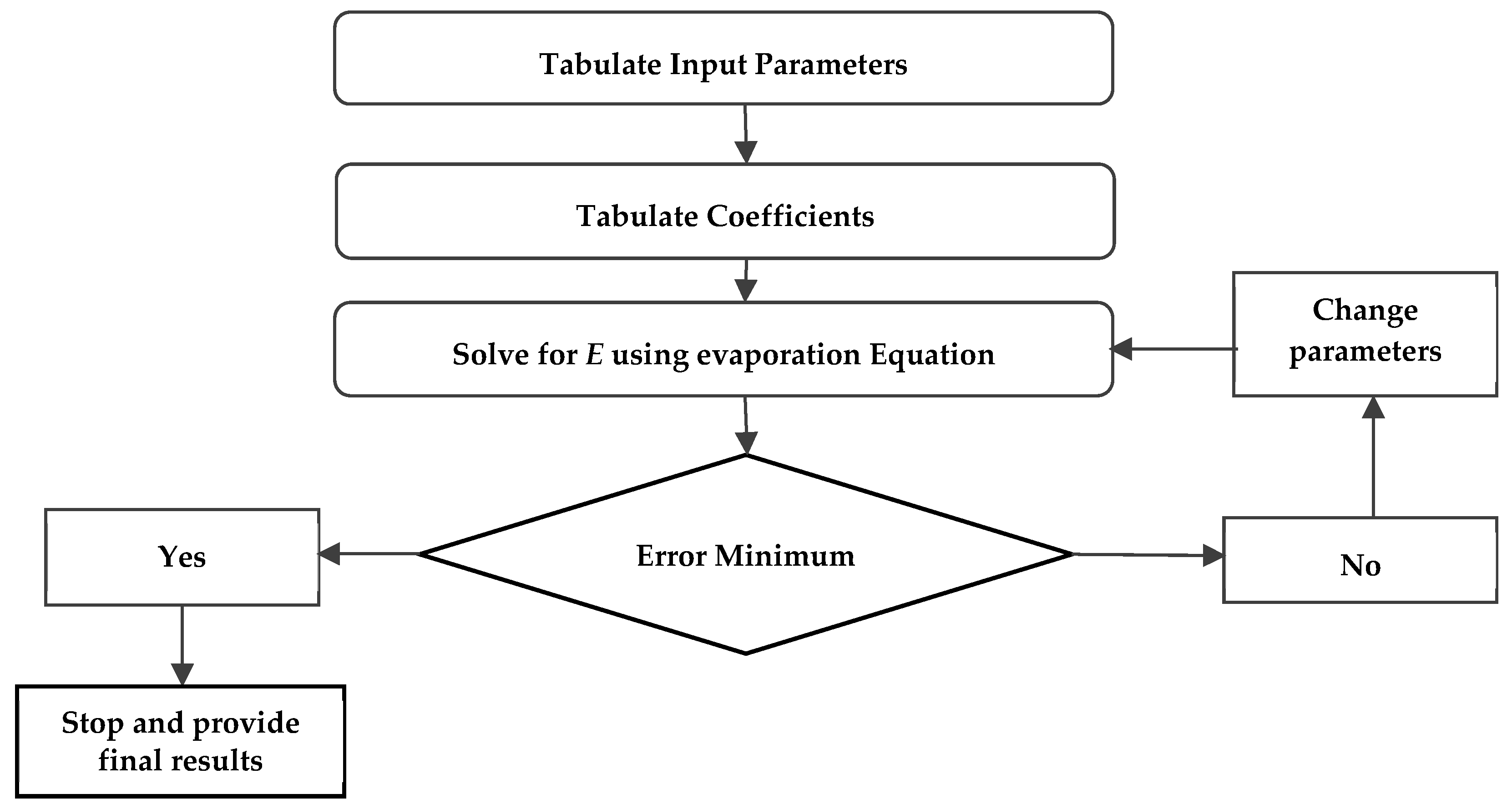
2.4.3. General Reduced Gradient (GRG) Method of Optimization

Using the abovementioned data, the ability of existing evaporation models to predict evaporation was examined and evaluated. Moreover, calibration of the adapted methods (Hamon, Penman, Jensen–Haise, and Makkink) was conducted based on actual measurements (20-year data), for a better evaporation modeling. Subsequently, validation of the developed evaporation equations was performed using different sets of actual evaporation measurements (the remaining 20 years of data).

There is a long history of using optimization techniques for solving nonlinear problems in hydrology. However, in the field of vaporization, its application is limited. One of the most common research methods includes finding the best values of hydraulic/hydrological parameters by searching for the global minimum value of an objective function (OF). The objective function might be estimated on the basis of common types of errors between the observed and simulated variables, such as evaporation in the present study. Usually, a search might result in multiple minimum values of an objective function, which are termed local minimums. However, the success of any optimization technique depends on finding the global minimum. In general, optimization can be summarized as maximizing or minimizing the OF:

$$OF=f\left(E\right)=\sum \left(C_i^a\right)\left(E_i^b\right),$$

(18)

where C₁, C₂, C₃, …, C_n are the objective function coefficients; E₁, E₂, E₃, …, E_n, or, in general, (E_i), are the decision variables (evaporation values); and ‘a’ and ‘b’ are any number. For example, if OF is the sum of squared errors between the simulated (s) and measured (m) values of evaporation (E_m(i) − E_s(i)), then b = 2, C_(i) = 1, and a = 1. The user might set a range of parameters used in the evaporation equation to estimate E_s(i). Another equation of the objective function might be in the form of any model-performance indicator, like the Nash–Sutcliffe efficiency, as explained below.

Nonlinear problems are inherently more difficult to solve than linear problems. There are a number of methods used in engineering to solve constrained nonlinear programming problems. This work used the GRG algorithm. The main reason for the use of this technique is that it is user-friendly and can efficiently converge to the global minimum solution [63]. The Generalized-Reduced-Gradient algorithm is one of the most robust methods. It is based on nonlinear programming [63]. A flowchart explaining the optimization is shown in Figure 3.

2.5. Performance Evaluation of Evaporation Equations

The accuracy of the equations was checked by the Nash–Sutcliffe efficiency (NSE) [64]:

$$NSE=\left(1-\frac{{\sum }_{i=1}^n{\left(E_{oi}-E_{si}\right)}^2}{{\sum }_{i=1}^n{\left(E_{oi}-{\overline{E}}_{oi}\right)}^2}\right),$$

(19)

where E_oi is the observed evaporation value of the ith data point, E_si is the simulated evaporation of the ith data point, ${\overline{E}}_{oi}$ is the average value of E_o, and n is the total number of observations used to develop the equation.

The other indicator used for testing the performance of the developed evaporation equations was the mean biased error (MBE):

$$MBE=\left(\frac{{\sum }_{i=1}^n\left(E_{si}-E_{oi}\right)}{n}\right).$$

(20)

The mean absolute error was also used in some cases.

3. Results and Discussion

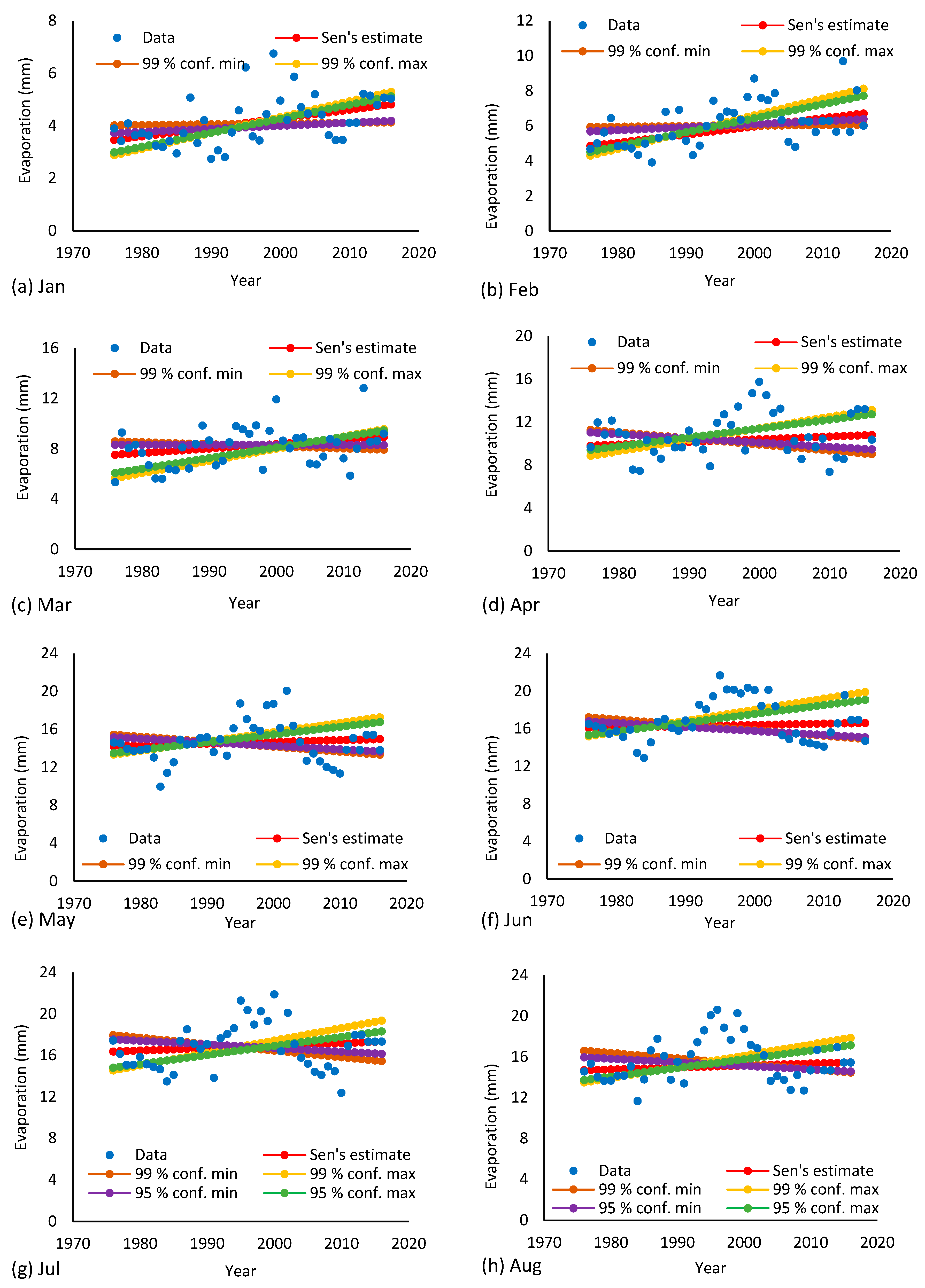
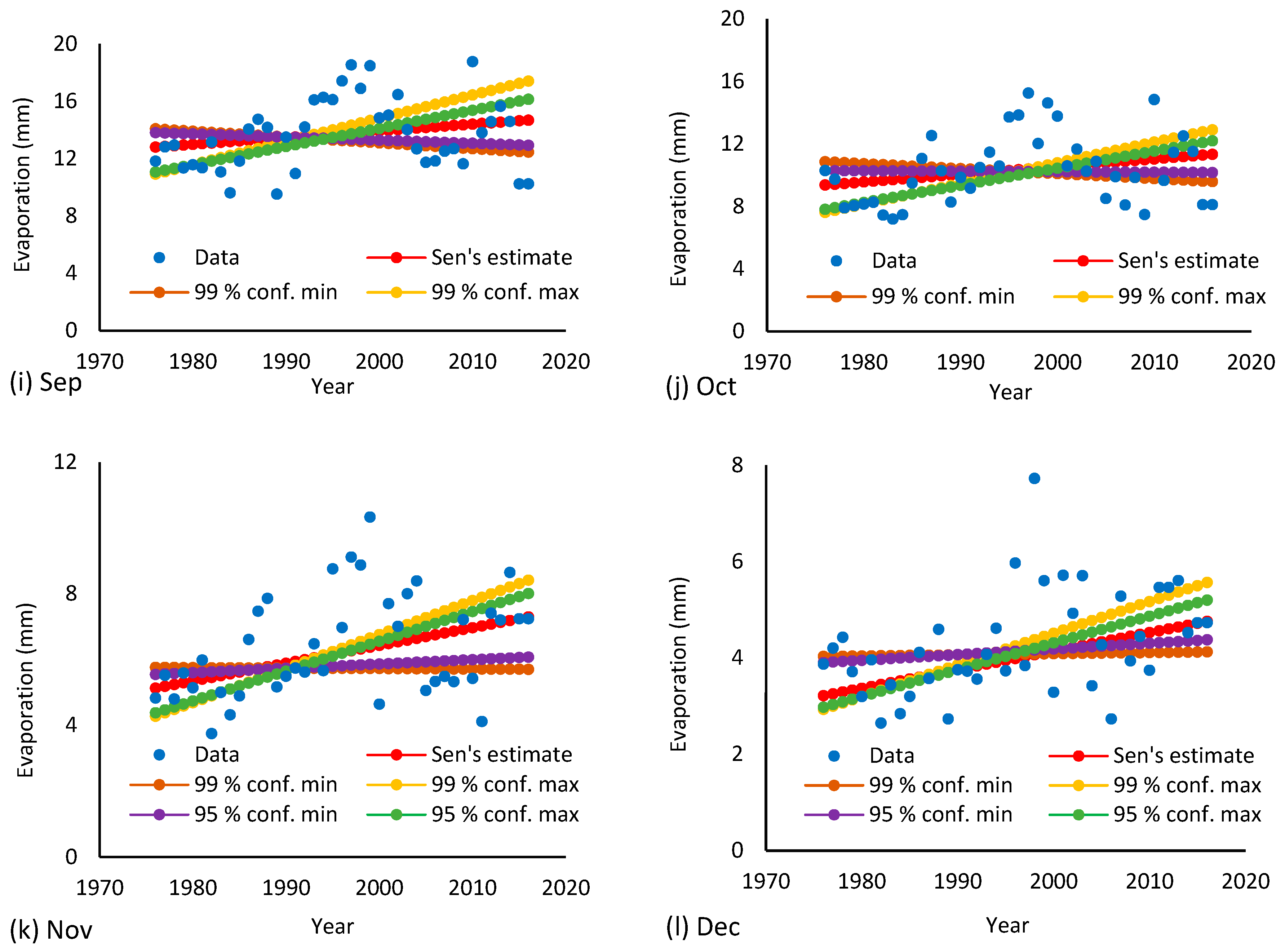
3.1. Data Analysis

The records of evaporation and meteorological data/parameters, including relative humidity, temperature, wind speed, and sunshine hours, were processed and are presented in graphical form in

Table 2. Daily/monthly evaporation and average daily temperature (average for the period 1976–2016).

Evaporation					Temperature
Month	Daily Maximum (mm)	Daily Minimum (mm)	Daily Average (mm)	Monthly (mm)	Average of Daily Maximum (°C)	Average of Daily Minimum (°C)	Daily Mean (°C)
Jan.	8.15	2.06	4.21	129.06	19.92	6.45	13.18
Feb.	9.55	3.18	6.14	171.33	22.88	8.45	15.67
Mar.	12.49	3.78	8.13	250.82	27.16	12.45	19.81
Apr.	16.31	4.73	10.72	322.82	32.94	17.46	25.20
May.	19.56	8.18	14.60	451.45	39.10	22.90	31.00
Jun.	20.75	12.95	16.88	504.02	42.55	24.99	33.77
Jul.	20.72	12.90	16.87	520.10	43.53	25.36	34.45
Aug.	19.27	12.22	15.80	485.51	43.77	25.59	34.68
Sep.	17.91	9.94	13.91	412.40	41.47	22.90	32.19
Oct.	14.94	6.61	10.56	322.62	35.91	17.93	26.92
Nov.	11.68	3.08	6.48	190.70	27.15	12.50	19.83
Dec.	8.08	2.23	4.28	131.94	21.70	8.32	15.01

. Before using the data for evaporation estimation, they were analyzed for trends. The Mann–Kendall and Sen’s slope tests were applied to investigate any trends in the evaporation data.

3.2. Data Analysis Results

The main data regarding evaporation estimation are presented in Section 3.1 in Table 2. It was observed that the mean daily evaporation was the maximum from May to September. The temperature was also the maximum during these months. The average daily evaporation ranged from 4.2 mm/day in January and December (winter) to 16.9 mm/day during summer. The maximum daily evaporation (mean of maximum daily evaporation for 40 years, from 1976 to 2016) ranged from 8.2 mm/day (winter) to 20.8 mm/day (summer).

The trend analysis results are given in

Table 3. Trend analysis results for evaporation (Z values).

Month	Jan.	Feb.	Mar.	Apr.	May.	Jun.	Jul.	Aug.	Sep.	Oct.	Nov.	Dec.
Z values	2.97	2.79	1.92	0.65	0.69	0.43	0.74	0.84	1.44	1.75	2.52	2.84
Trend	Yes	Yes	No	No	No	No	No	No	No	No	Yes	Yes

and Figure 4. It was noticed that there was a positive trend in evaporation for the months of January, February, November, and December. There was no trend in the months of high evaporation during summer, so the data could be used for estimations of evaporation. The trends of only a few months would not affect the results of the evaporation equations. It is worth mentioning here that the equations would have limitations for producing high accuracy results during the months of January, February, November, and December, because the whole data from all months over the calibration and validation periods were used without removing the trend component of the data. However, the results related to the months of high evaporation could be considered to be reasonably accurate, as there was no trend in evaporation for these months.

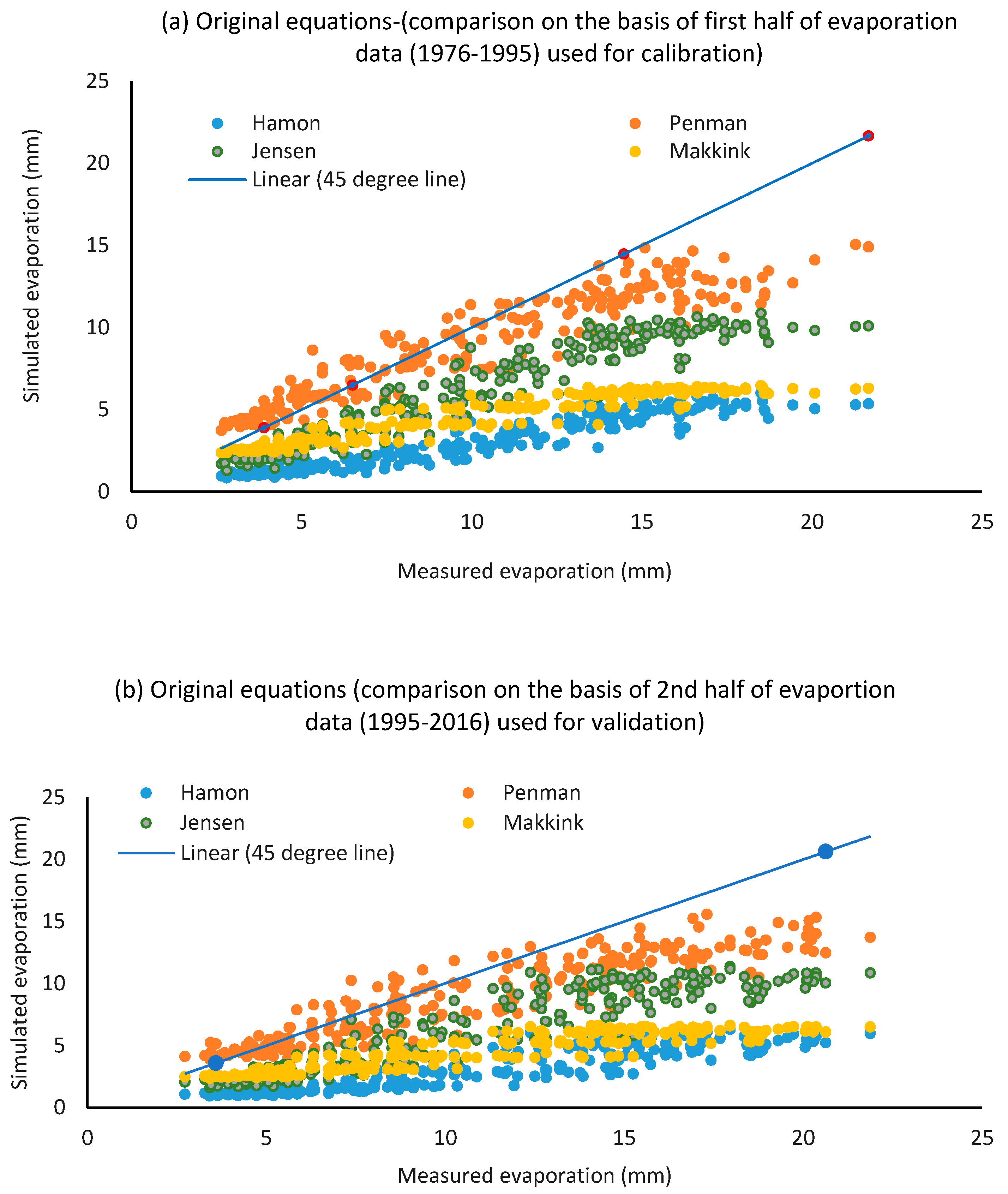
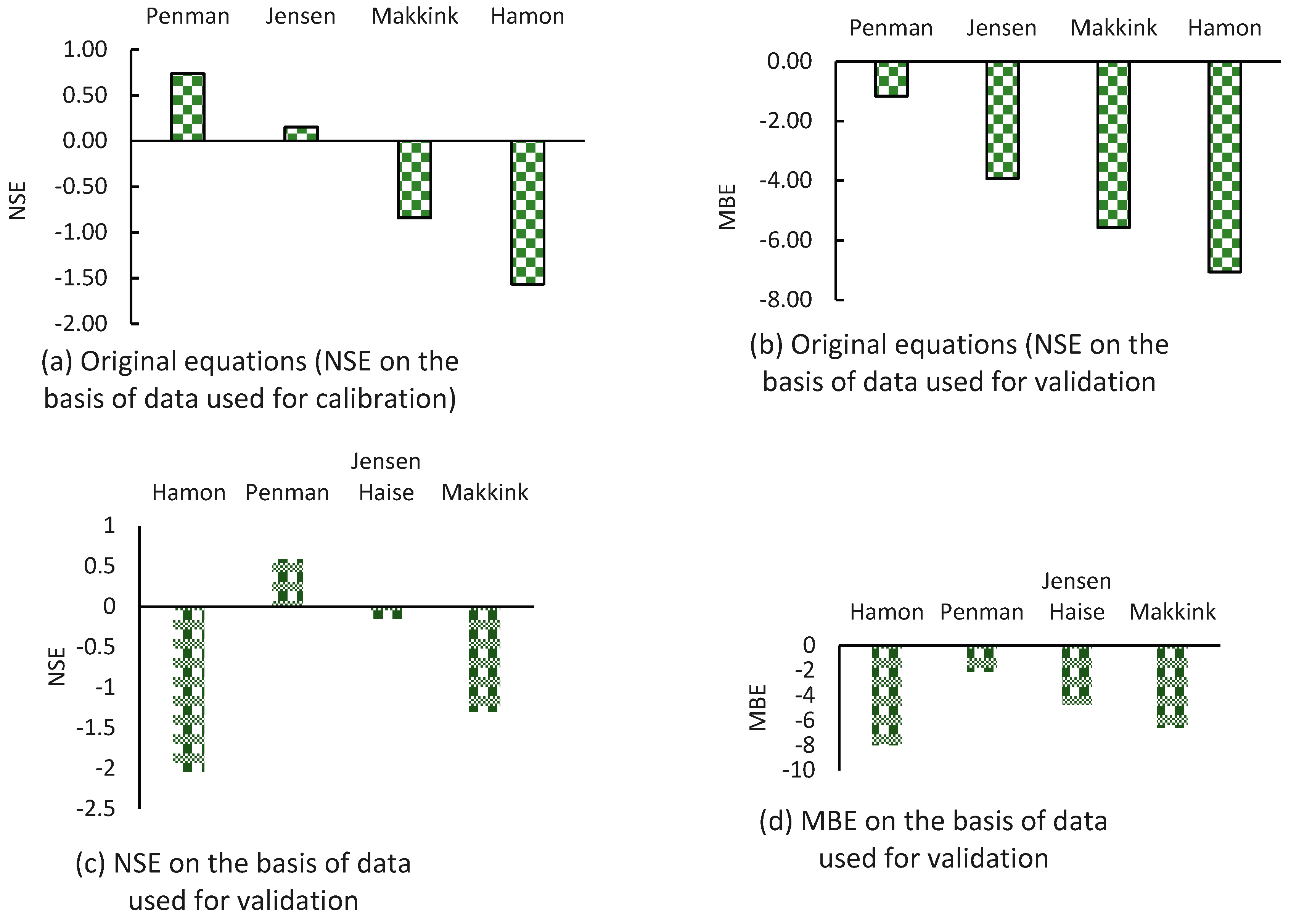
3.3. Comparison of Evaporation Simulated by Various Equations

A comparison of the four equations on the basis of pan evaporation is presented in Figure 5a,b and Figure 6a,b. The blue line in Figure 5a,b represents the 45° line. The results closest to this line are the best results. Points below this line represent the underestimated results and the overestimated values are displayed above this line. This shows that the performance of the Penman equation was better than the other three equations. These results match the results found by Said and Hussein in 2013 [10]. Merit-wise, these equations can be placed as Penman (merit number 1), Jensen–Haise (2), Makkink (3), and Hamon (4). The results of simulated evaporation were only close to the 45° line for the Penman equation. The results from the other equations were far from the 45° line. The Nash–Sutcliffe coefficients for the Penman, Jensen–Haise, Makkink, and Hamon equations were 0.74, 0.15, −0.84, and −1.57, respectively. The MBE values for the Penman, Jensen–Haise, Makkink, and Hamon equations were –1.16, −3.93, −5.57, and −7.06 mm, respectively (Figure 6). Acceptable NSE values were taken as greater than 0.5. This means that only the Penman equation met the accuracy criteria, although it also slightly underestimated evaporation compared to the measured values, as shown by the MBE values. The reason for the better performance of the Penman equation is that it involves, to some extent, the physics of the evaporation phenomenon. It includes temperature, wind speed, sun shine hours, and net radiation as input data. It combines the fixed bulk surface resistance and vapor aerodynamic (combines the mass-transfer and energy-budget approaches), which implicitly generates a strong theoretical basis [43]. It is worth mentioning here that the merit of equations determined in this research is on the basis of specific pan evaporation and other meteorological data.

All four equations are of an empirical nature and the accuracy of their output depends upon the closeness of the data to that on the basis of which these equations were developed. According to Lu et al. [65], for hot and dry areas, the differences in estimated evaporation obtained by various methods exceeded 700 mm/year. Other researchers have also reported that the performance of these equations depends on the nature of the data. Nagai [56] estimated pan evaporation by the Makkink equation and found that the results are very close to those of the Penman equation. However, he concluded that for the best results of the evaporation estimation, there is a need to calibrate the empirical constants of the equations on the basis of the data for a specific region. In other research [66], it was concluded that the Makkink equation produces better results of estimation of evaporation compared to those of the Jensen–Haise equation. Fernandes [67] also found similar results. He [67] compared simple equations based on only temperature and found an acceptable performance for the Hamon equation.

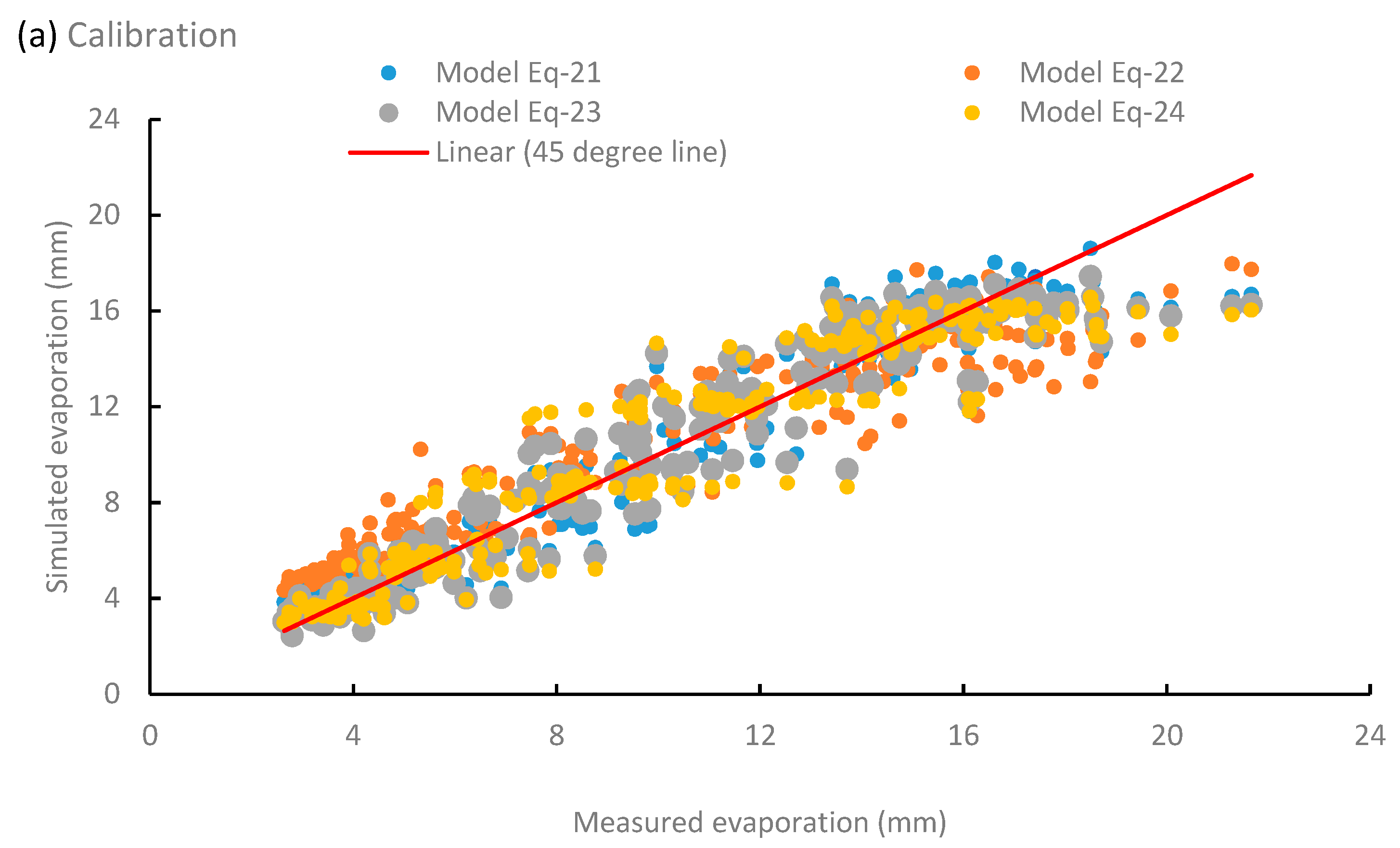
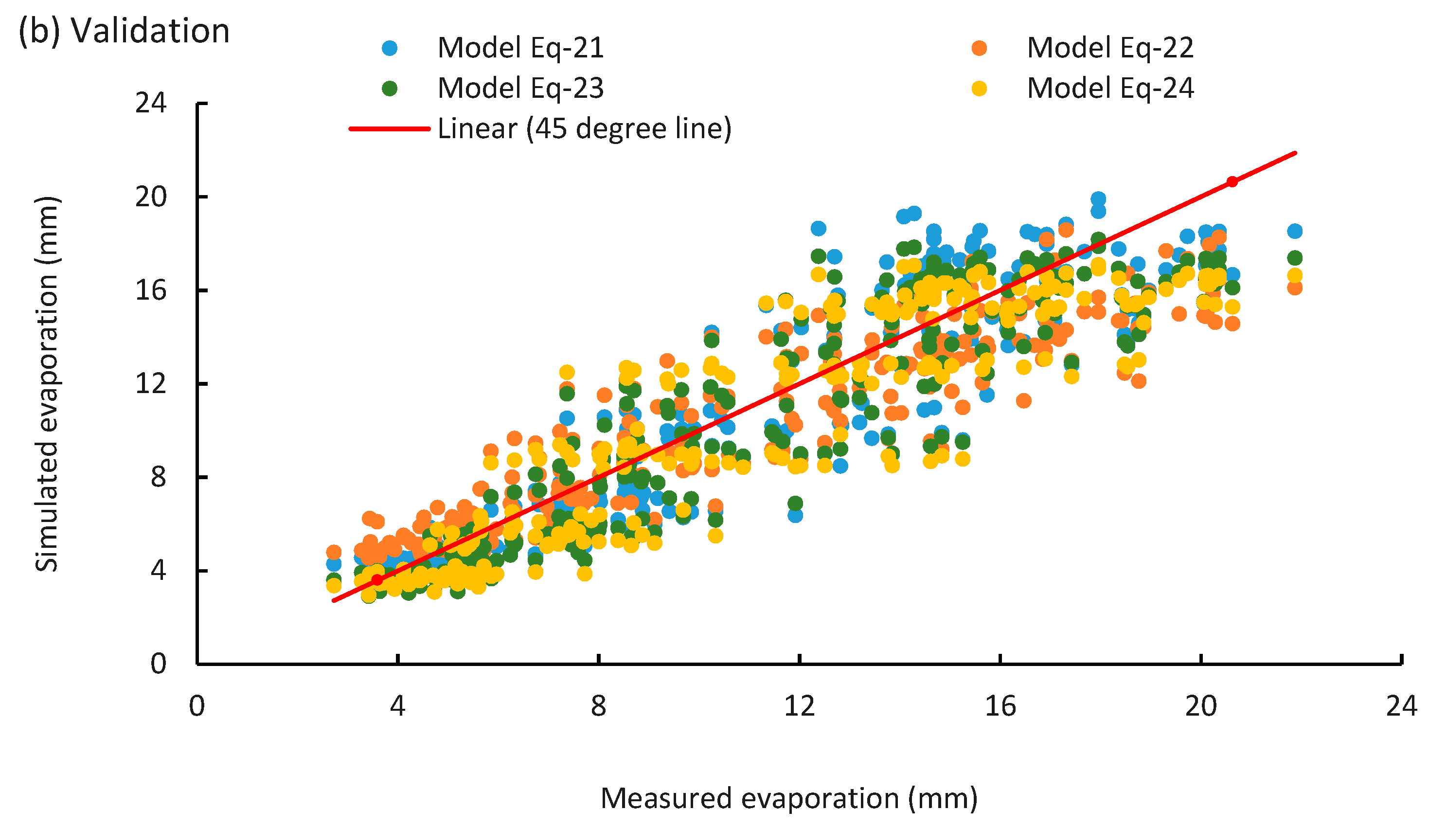
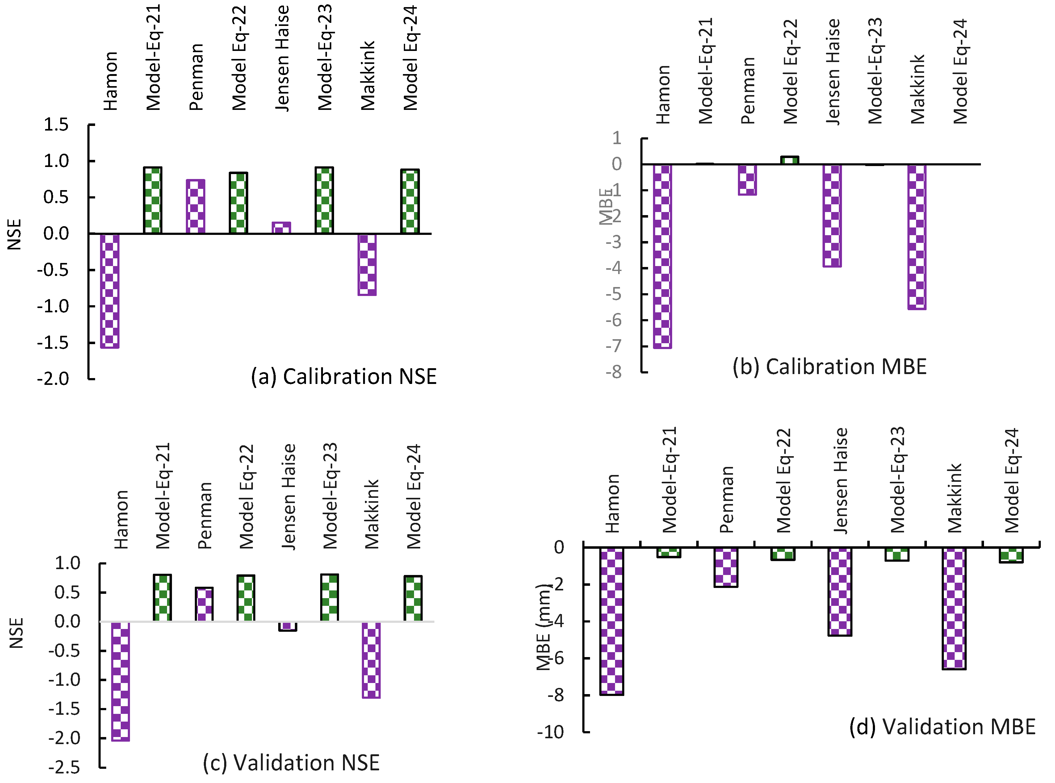
3.4. Calibration and Validation of the Developed Equations

The results of optimization on the basis of three objective functions were checked and it was found that the objective function based on NSE gave better results compared to the results produced by using the MBE as the objective function. The NSE value was 27% higher in the case of maximizing the NSE, compared to the NSE value obtained by minimizing the MBE. However, optimization using the objective function based on the mean absolute error produced values of optimized parameters and performance indicators similar to those produced by using NSE as the objective function. The objective function based on the NSE was finally used to identify the parameters for developing new evaporation equations. The Albedo coefficient used to estimate R_ns in the case of the Penman Equation (Equation (3)) and Jensen–Haise Equation (Equation (8)) played an important role in the calibration process. Its initial value was provided as 0.23 to start the calibration and the final value was obtained as 0.163, for this coefficient.

The results from the four developed equations are presented in Figure 7a,b and Figure 8. It can be seen that the application of optimization resulted in improved equations. The evaporation estimated by all four newly developed equations was highly accurate, i.e., the results were very close to the 45° line. It is worth noting that such results are hardly reported in the literature (see [2,5,8,10,31,32]). Figure 8a–d shows the calibration and validation results for both the original and newly developed equations in terms of NSE and MBE. These results indicated that the developed equations performed much better than the original equations. The NSE, MBE, and an additional indicator (mean absolute error) presented in

Table 4. Absolute error in the case of calibration and validation.

Error	Hamon Method	Penman Method	Jensen–Haise Method	Makkink Method
Maximum Absolute Error (mm)	5.66	6.66	5.76	6.48
Minimum Absolute Error (mm)	−6.25	−4.41	−5.07	−5.11
Average Absolute Error (mm)	1.75	1.80	1.75	1.84

showed that the NSE values for all of the developed equations were greater than 0.5 (i.e., an acceptable value). In the case of calibration, the NSE values were 0.91, 0.84, 0.91, and 0.88 for Equation (1) (Hamon), Equation (2) (Penman), Equation (3) (Jensen–Haise), and Equation (4) (Makkink), while the MBE values were found to be 0.02, 0.29, −0.02, and 0.0 for the same equations, respectively. For the validation process, the NSE values were 0.8, 0.79, 0.81, and 0.78 for Equation (1) (Hamon), Equation (2) (Penman), Equation (3) (Jensen–Haise), and Equation (4) (Makkink), and the MBE values were −0.52, −0.67, −0.71, and −0.81 for these equations, respectively. The calibration process revealed that the equations depending upon a single variable or just a few variables (e.g., temperature only or temperature and humidity only) were easy and more efficient. For instance, the Hamon equation only depends on temperature and its calibration and validation results were found to be more reliable in comparison to the other equations. However, such equations are not robust and are highly data-dependent. The original form of the same equation produced the worst results, as it was developed using a certain set of data. The final developed equations using optimization are given below.

The developed equation on the basis of the Hamon method:

$$E=2.38 D^{1.75} {10}^{\left(\frac{6.86 T_a}{T_a+273}\right)}.$$

(21)

The developed equation on the basis of the Penman method with an Albedo coefficient equal to 0.23:

$$E=\frac{\mathsf{\Delta }}{\mathsf{\Delta }+\gamma }\frac{R_{net}}{\lambda }+\frac{\gamma }{\mathsf{\Delta }+\gamma }0.0026\left(1+0.728\overline{u}\right)\left(1-r\right)e_{sa}n.$$

(22)

The developed equation on the basis of the Jensen–Haise method:

$$E=\left[0.016\left(2.2 T_a+32\right)-0.53\right]\frac{R_{ns}}{\lambda }.$$

(23)

The developed equation on the basis of the Makkink method:

$$E=1.86\frac{\mathsf{\Delta }}{\mathsf{\Delta }+\gamma }\frac{R_{ns}}{\lambda }-4.97.$$

(24)

4. Summary and Conclusions

Extensive records of pan evaporation, temperature, relative humidity, and sunshine hours were used in the present research for the analysis and development of evaporation equations. Data analysis using the Mann–Kendall and Sen’s slope tests found a specific trend for evaporation in the Qassim Region, for the months of January, February, November, and December (i.e., primarily the winter season). The summer months, with the maximum evaporation, showed no trends based on the measured evaporation records.

Evaporation was estimated using four different methods: The Hamon, Penman, Jensen–Haise, and Makkink equations. The results of these four equations were compared on the basis of extensive measured data regarding pan evaporation, temperature, relative humidity, and sunshine hours. It was concluded that the Penman equation was robust and provided estimates of pan evaporation with a reasonably acceptable accuracy. Its performance was found to be better than that of the other three equations.

Optimization using three different objective functions was applied to develop a more accurate set of evaporation equations. The objective function based on NSE gave much better results, compared to the objective function based on MBE (NSE value 27% higher). The objective function based on the mean absolute error produced values of optimized parameters and performance indicators similar to those produced by NSE. Four equations on the basis of the Hamon, Penman, Jensen–Haise, and Makkink equations were developed for the Al Qassim Region. The parameters of the four equations were optimized using the GRG optimization method. The optimization helped to find equations to estimate evaporation in Qassim with a high accuracy (NSE in the range of 0.8–0.9).

An important conclusion of this research was regarding the Albedo coefficient. Its value had a significant impact on the estimated values of evaporation obtained from various equations. The Albedo coefficient found with the help of optimization was 0.163 for the Qassim Region.

It might be noted that a general methodology was developed for parameter optimization for evaporation equations in this research. Although the methodology was applied to the case of the Qassim Region, it could be used anywhere in the world with similar conditions, if sufficiently long records for evaporation and meteorological data are available for model calibration and verification.

References

1. Tarawneh, Q.Y.; Chowdhury, S. Trends of Climate Change in Saudi Arabia: Implications on Water Resources. Climate 2018, 6, 8. [Google Scholar] [CrossRef] [Green Version]
2. Yang, Y.; Roderick, M.L. Radiation, Surface Temperature and Evaporation Over Wet Surfaces. Q. J. R. Meteorol. Soc. 2019, 145, 1118–1129. [Google Scholar] [CrossRef]
3. Stassen, C.; Dommenget, D.; Loveday, N. A Hydrological Cycle Model for the Globally Resolved Energy Balance (GREB) model v1.0. Geosci. Model Dev. 2019, 12, 425–440. [Google Scholar] [CrossRef] [Green Version]
4. Wang, B.; Ma, Y.; Ma, W.; Su, B.; Dong, X. Evaluation of Ten Methods for Estimating Evaporation in a Small High-Elevation Lake on the Tibetan Plateau. Appl. Clim. 2019, 136, 1033–1045. [Google Scholar] [CrossRef]
5. Ahmadipour, A.; Shaibani, P.; Mostafavi, S.A. Assessment of Empirical Methods for Estimating Potential Evapotranspiration in Zabol Synoptic Station by REF-ET Model. Medbiotech J. 2019, 3, 1–4. [Google Scholar]
6. Zolá, R.P.; Bengtsson, L.; Berndtsson, R.; Martí-Cardona, B.; Satgé, F.; Timouk, F.; Bonnet, M.P.; Mollericon, L.; Gamarra, C.; Pasapera, J. Modelling Lake Titicaca’s Daily and Monthly Evaporation. Hydrol. Earth Syst. Sci. 2019, 23, 657–668. [Google Scholar] [CrossRef] [Green Version]
7. Al-Domany, M.; Touchart, L.; Bartout, P.; Choffel, Q. Direct Measurements and a New Mathematical Method to Estimate the Pond Evaporation of the French Midwest. Appl. Sci. Innov. Res. 2018, 2, 1–24. [Google Scholar] [CrossRef] [Green Version]
8. Duan, Z.; Bastiaanssen, W.G.M. Evaluation of Three Energy Balance-Based Evaporation Models for Estimating Monthly Evaporation for Five Lakes Using Derived Heat Storage Changes from a Hysteresis Model. Environ. Res. Lett. 2017, 12, 4005. [Google Scholar] [CrossRef] [Green Version]
9. Scavo, F.B.; Tina, G.M.; Gagliano, A. Comparison of Evaporation Models for Free Water Basins Surfaces. In Proceedings of the 4th International Conference on Smart and Sustainable Technologies (SpliTech), Split, Croatia, 18–21 June 2019. [Google Scholar] [CrossRef]
10. Said, M.A.; Hussein, M.M.A. Estimation of Evaporation from Lake Burullus (Egypt) Using Different Techniques. J. King Abdel Aziz Univ. Mar. Sci. 2013, 24, 55–67. [Google Scholar] [CrossRef]
11. Crago, R.D.; Brutsaert, W.A. Comparison of Several Evaporation Equations. Water Resour. Res. 1992, 28, 951–954. [Google Scholar] [CrossRef]
12. Hussein, M.M.A. Evaluation of Alexandria Eastern Harbor Evaporation Estimate Methods. Water Resour. Manag. 2015, 29, 3711. [Google Scholar] [CrossRef]
13. Patel, J.A.; Majmundar, B.P. Development of Evaporation Estimation Methods for a Reservoir in Gujarat, India. Am. Water Works Assoc. 2016, 108, E489–E500. [Google Scholar] [CrossRef]
14. Yan, Z.; Wang, S.; Ma, D.; Liu, B.; Lin, H.; Li, S. Meteorological Factors Affecting Pan Evaporation in the Haihe River Basin, China. Water 2019, 11, 317. [Google Scholar] [CrossRef] [Green Version]
15. Bhatt, R.; Hossain, A. Concept and Consequence of Evapotranspiration for Sustainable Crop Production in the Era of Climate Change. Adv. Evapotranspiration Methods Appl. 2019. [Google Scholar] [CrossRef] [Green Version]
16. Meng, W.; Sun, X.; Ma, J.; Guo, X.; Zheng, L. Evaporation and Soil Surface Resistance of the Water Storage Pit Irrigation Trees in the Loess Plateau. Water 2019, 11, 648. [Google Scholar] [CrossRef] [Green Version]
17. Lu, Z.; Kinefuchi, I.; Wilke, K.L.; Vaartstra, G.; Wang, E.N. A Unified Relationship for Evaporation Kinetics at Low Mach Numbers. Nat. Commun. 2019, 10, 2368. [Google Scholar] [CrossRef] [Green Version]
18. Rayner, D.P. Wind Run Changes: The Dominant Factor Affecting Pan Evaporation Trends in Australia. J. Clim. 2007, 20, 3379–3394. [Google Scholar] [CrossRef]
19. Cummings, N.W.; Richardson, B. Evaporation from Lakes. Phys. Rev. 1927, 30, 527. [Google Scholar] [CrossRef]
20. Majidi, M.; Alizadeh, A.; Farid, A.; Vazifedoust, M. Estimating Evaporation from Lakes and Reservoirs under Limited Data Condition in a Semi-Arid Region. Water Resour. Manag. 2015, 29, 3711. [Google Scholar] [CrossRef]
21. Andersen, M.E.; Jobson, H.E. Comparison of Techniques for Estimating Annual Lake Evaporation Using Climatological Data. Water Resour. Res. 1982, 18, 630–636. [Google Scholar] [CrossRef]
22. Penman, H.L. Natural Evaporation from Open Water, Bare Soil, and Grass. Proc. R. Soc. 1948, 76, 372–383. [Google Scholar]
23. Upadhyaya, A. Comparison of Different Methods to Estimate Mean Daily Evapotranspiration from Weekly Data at Patna, India. Irrig. Drain. Syst. Eng. 2006, 5, 1–7. [Google Scholar]
24. Assouline, S.; Mahrer, Y. Evaporation from Lake Kinneret 1: Eddy Correlation System Measurements and Energy Budget Estimates. Water Resour. Res. 1993, 29, 901–910. [Google Scholar] [CrossRef]
25. Collison, J.W. The Collison Floating Evaporation Pan: Design, Validation, and Comparison. 2019. Available online: https://digitalrepository.unm.edu/ce_etds/233 (accessed on 23 October 2019).
26. Tanny, J.; Cohen, S.; Assouline, S.; Lange, F.; Grava, A.; Berger, D.; Teltch, B.; Parlange, M.B. Evaporation from a Small Water Reservoir: Direct Measurements and Estimates. J. Hydrol. 2008, 351, 218–229. [Google Scholar] [CrossRef] [Green Version]
27. Chu, C.R.; Li, M.H.; Chang, Y.F.; Liu, T.C.; Chen, Y.Y. Wind-Induced Splash in Class a Evaporation Pan. J. Geophys. Res. 2012, 117, D11101. [Google Scholar] [CrossRef]
28. Morton, F.I. Catchment Evaporation and Potential Evaporation Further Development of a Climatological Relationship. J. Hydrol. 1971, 12, 81–99. [Google Scholar] [CrossRef]
29. Yao, H.; Creed, I.F. Determining Spatially Distributed Annual Water Balances for Un-Gauged Locations on Shikoku Island, Japan: A Comparison of Two Interpolators. Hydrol. Sci. J. 2005, 50, 245–263. [Google Scholar] [CrossRef]
30. Winter, T.C.; Rosenberry, D.O.; Sturrock, A.M. Evaluation of 11 Equations for Determining Evaporation for a Small Lake in The North Central United States. Water Resour. Res. 1995, 31, 983–993. [Google Scholar] [CrossRef]
31. Winter, T.; Buso, D.; Rosenberry, D.; Likens, G.; Sturrock, A., Jr.; Mau, D. Evaporation determined by the energy budget method for Mirror Lake, New Hampshire. Limnol. Oceanogr. 2003, 48, 995–1009. [Google Scholar] [CrossRef] [Green Version]
32. Moazed, H.; Ghaemii, A.A.; Rafiee, M.R. Evaluation of Several Reference Evapotranspiration Methods: A Comparative Study of Greenhouse and Outdoor Conditions. Trans. Civ. Eng. 2014, 38, 421. [Google Scholar]
33. Paparrizos, S.; Maris, F.; Matzarakis, A. Estimation and Comparison of Potential Evapotranspiration Based on Daily and Monthly Data from Sperchios Valley in Central Greece. Glob. Nest J. 2014, 16, 204–217. [Google Scholar]
34. Anderson, R.J.; Smith, S.D. Evaporation Coefficient for the Sea Surface from Eddy Flux. J. Geophys. Res. 1981, 86, 449–456. [Google Scholar] [CrossRef]
35. Djaman, K.; Balde, A.B.; Sow, A.; Muller, B.; Irmak, S.; N’Diaye, M.K.; Manneh, B.; Moukoumbi, Y.D.; Futakuchi, K.; Saito, K. Evaluation of Sixteen Reference Evapotranspiration Methods under Sahelian Conditions in the Senegal River Valley. J. Hydrol. Reg. Stud. 2015, 3, 139–159. [Google Scholar] [CrossRef] [Green Version]
36. Song, X.; Lu, F.; Xiao, W.; Zhu, K.; Zhou, Y.; Xie, Z. Performance of Twelve Reference Evapotranspiration Estimation Methods to Penman-Monteith Method and the Potential Influences in Northeast China. Meteorol. Appl. 2019, 26, 83–96. [Google Scholar] [CrossRef] [Green Version]
37. Hosseinzadeh, T.P.; Tabari, H.; Abghari, H. Pan Evaporation and Reference Evapotranspiration Trend Detection in Western Iran with Consideration of Data Persistence. Hydrol. Res. 2014, 45, 213–225. [Google Scholar] [CrossRef]
38. Lee, T.; Najim, M.; Aminul, M. Estimating Evapotranspiration of Irrigated Rice at the West Coast of the Peninsular of Malaysia. J. Appl. Irrig. Sci. 2004, 39, 103–117. [Google Scholar]
39. Muniandy, J.M.; Yusop, Z.; Askari, M. Evaluation of Reference Evapotranspiration Models and Determination of Crop Coefficient for Momordica Charantia and Capsicum Annuum. Agric. Water Manag. 2016, 169, 77–89. [Google Scholar] [CrossRef]
40. Ali, M.H.; Lee, T.; Kwok, C.; Eloubaidy, A.F. Modelling Evaporation and Evapotranspiration under Temperature Change in Malaysia. Pertanika J. Sci. Technol. 2000, 8, 191–204. [Google Scholar]
41. Ali, M.H.; Shui, L.T. Potential Evapotranspiration Model for Muda Irrigation Project, Malaysia. Water Resour. Manag. 2008, 23, 57. [Google Scholar] [CrossRef]
42. Allen, R.G.; Pereira, L.S.; Raes, D.; Smith, M. Crop Evapotranspiration-Guidelines for Computing Crop Water Requirements-FAO Irrigation and Drainage Paper 56; FAO: Rome, Italy, 1998; Volume 300, p. D05109. [Google Scholar]
43. Tukimat, N.N.A.; Harun, S.; Shahid, S. Comparison of Different Methods in Estimating Potential Evapotranspiration at Muda Irrigation Scheme of Malaysia. J. Agric. Rural Dev. Trop. Subtrop. 2012, 113, 77–85. [Google Scholar]
44. Doorenbos, J.; Pruitt, W. Crop Water Requirements; FAO Irrigation and Drainage Paper 24; FAO Land and Water Development Division: Rome, Italy, 1977; pp. 1–144. [Google Scholar]
45. Stull, R.B. An Introduction to Boundary Layer Meteorology; Kluwer Academic Publishers: Dordrecht, The Netherlands, 1988. [Google Scholar]
46. Hamon, W.R. Estimating Potential Evapotranspiration. J. Hydraul. Div. Proc. Am. Soc. Civ. Eng. 1963, 871, 107–120. [Google Scholar]
47. Lang, D.; Zheng, Z.; Shi, J.; Liao, F.; Ma, X.; Wang, W.; Chen, X.; Zhang, M. A Comparative Study of Potential Evapotranspiration Estimation by Eight Methods with FAO Penman–Monteith Method in Southwestern China. Water 2017, 7, 734. [Google Scholar] [CrossRef] [Green Version]
48. Doorenbus, J.; Pruitt, W.O. Guidelines for Predicting Crop Water Requirements, Irrigation and Drainage Paper; Food and Agriculture Organization of the United Nations: Rome, Italy, 1977. [Google Scholar]
49. Alazrd, M.; Leduc, C.; Travi, Y.; Boulet, G.; Ben Salem, A. Estimating Evaporation in Semi-Arid Areas Facing Data Scarcity: Examples of the El Haouraeb Dam (Merguellil catchment, Central Tunisia). J. Hydrol. Reg. Stud. 2015, 3, 265–284. [Google Scholar] [CrossRef] [Green Version]
50. Yao, H.; Terakawa, A.; Chen, S. Rice Water Use and Response to Potential Climate Changes: Calculation and Application to Jianghan, China. In Proceedings of the International Conference on Water Resources and Environment Research, Kyoto, Japan, 5–9 June 1996; Volume 2, pp. 611–618. [Google Scholar]
51. Souch, C.; Wolfe, C.P.; Susan, C.; Grimmond, B. Wetland Evaporation and Energy Partitioning: Indiana Dunes National Lakeshore. J. Hydrol. 1996, 184, 189–208. [Google Scholar] [CrossRef]
52. Valiantzas, J.D. Simplified Version for the Penman Evaporation Equation Using Routine Weather Data. J. Hydrol. 2006, 331, 690–702. [Google Scholar] [CrossRef]
53. Vardavas, I.M. Modeling the Seasonal Radiation of Net All-Wave Radiation Flux and Evaporation in a Tropical Wet-Dry Region. Ecol. Modell. 1987, 39, 247–268. [Google Scholar] [CrossRef]
54. Vardvas, I.M.; Fountoulakis, A. Estimation of Lake Evaporation from Standard Meteorological Measurements: Application to Four Australian Lakes in Different Climatic Regions. Ecol. Modell. 1996, 84, 139–150. [Google Scholar] [CrossRef]
55. Jensen, M.E.; Hake, H.R. Estimating Evapotranspiration from Solar Radiation. J. Irrig. Drain. Div. 1963, 96, 25–28. [Google Scholar]
56. Nagai, A. Estimation of Pan Evaporation by Makkink Equation. J. Jpn. Soc. Hydrol. Water Resour. 1993, 6, 238–243. [Google Scholar] [CrossRef]
57. Mann, H.B. Non-Parametric Tests against Trend. Econmetrica 1945, 13, 245–259. [Google Scholar] [CrossRef]
58. Kendall, M.G. Rank Correlation Methods; Charles, G., Ed.; Griffin: London, UK, 1975. [Google Scholar]
59. Sen, P.K. Estimates of the Regression Coefficient Based on Kendall’s Test. J. Am. Stat. Assoc. 1968, 63, 1379–1389. [Google Scholar] [CrossRef]
60. Rathnayake, U. Comparison of Statistical Methods to Graphical Methods in Rainfall Trend Analysis: Case Studies from Tropical Catchments. Adv. Meteorol. 2019. [Google Scholar] [CrossRef] [Green Version]
61. Ali, R.O.; Abubaker, S.H. Trend Analysis Using Mann-Kendall, Sen’s Slope Estimator Test and Innovative Trend Analysis Method in River Basin, China: Review. Int. J. Eng. Technol. 2019, 8, 110–119. [Google Scholar]
62. Totaro, V.; Gioia, A.; Iacobellis, V. Power of Parametric and Non-Parametric Tests for Trend Detection in Annual Maximum Series. Hydrol. Earth Syst. Sci. 2019, 2019, 8603586. [Google Scholar] [CrossRef] [Green Version]
63. Zhou, Y.; Yang, B.; Han, J.; Huang, Y. Robust Linear Programming and Its Application to Water and Environmental Decision-Making under Uncertainty. Sustainability 2019, 11, 33. [Google Scholar] [CrossRef] [Green Version]
64. Nash, J.E.; Sutcliffe, J.V. River Flow Forecasting Through Conceptual Models, Part I—A Discussion of Principles. J. Hydrol. 1970, 10, 282–290. [Google Scholar] [CrossRef]
65. Lu, J.; Sun, G.; McNulty, S.; Amatya, D.M.A. Comparison of Six Potential Evapotranspiration Methods for Regional Use in the Southeastern United States. J. Am. Water Resour. Assoc. 2005, 41, 621–633. [Google Scholar] [CrossRef]
66. Poyen, F.B.; Ghosh, A.K.; Kundu, P. Review on Different Evapotranspiration Empirical Equations. Int. J. Adv. Eng. Manag. Sci. 2016, 2, 17–24. [Google Scholar]
67. Fernandes, L.C.; Paiva, C.M.; Filho, O.C.R. Evaluation of Six Empirical Evapotranspiration Equations—Case Study. Rev. Bras. Meteorol. 2012, 27, 272–280. [Google Scholar] [CrossRef] [Green Version]
Figure 1. Framework for the methodology.
Water 12 00228 g001
Figure 2. Map showing the location of the Weather Station in Qassim Region in the Kingdom of Saudi Arabia.
Water 12 00228 g002
Figure 3. Flow Chart of the General Reduced Gradient Method of Optimization.
Water 12 00228 g003
Figure 4. Trends of evaporation data in the month of: (a) January; (b) February; (c) March; (d) April; (e) May; (f) June; (g) July; (h) August; (i) September; (j) October; (k) November; and (l) December.
Water 12 00228 g004aWater 12 00228 g004b
Figure 5. Comparison of the observed and simulated values of evaporation obtained from the four equations: (a) Original equations—half data; and (b) original equations—second half data.
Water 12 00228 g005
Figure 6. Error values for simulated evaporation obtained from various original equations: (a) Nash and Sutcliffe Efficiency (NSE) for data used in calibration, (b) Mean Biased Error (MBE) for data used in calibration, (c) NSE for data used in validation, and (d) MBE for data used in validation.
Water 12 00228 g006
Figure 7. Comparison of the observed and simulated values of evaporation obtained from the four developed equations: (a) Calibration; and (b) Validation.
Water 12 00228 g007aWater 12 00228 g007b
Figure 8. NSE and MBE values for simulated evaporation from the various developed equations: (a) Calibration NSE; (b) Calibration MBE; (c) Validation NSE; and (d) Validation MBE.
Water 12 00228 g008