Modeling River Ice Breakup Dates by k-Nearest Neighbor Ensemble

Abstract

Forecasting of river ice breakup timing is directly related to the local ice-caused flooding management. However, river ice forecasting using k-nearest neighbor (kNN) algorithms is limited. Thus, a kNN stacking ensemble learning (KSEL) method was developed and applied to forecasting breakup dates (BDs) for the Athabasca River at Fort McMurray in Canada. The kNN base models with diverse inputs and distance functions were developed and their outputs were further combined. The performance of these models was examined using the leave-one-out cross validation method based on the historical BDs and corresponding climate and river conditions in 1980–2015. The results indicated that the kNN with the Chebychev distance functions generally outperformed other kNN base models. Through the simple average methods, the ensemble kNN models using multiple-type (Mahalanobis and Chebychev) distance functions had the overall optimal performance among all models. The improved performance indicates that the kNN ensemble is a promising tool for river ice forecasting. The structure of optimal models also implies that the breakup timing is mainly linked with temperature and water flow conditions before breakup as well as during and just after freeze up.

1. Introduction

As an important annual event in northern high-latitude regions, general public and water resources managers are concerned about the river ice breakup every spring [1,2,3,4]. This is because breakup in late winter may cause annual peak water levels and possible ice-associated flooding risks, which may further result in extensive infrastructure damage and substantial financial losses [5,6]. Among the variables of interest in winter flooding management, the breakup date is critical since its early accurate forecasting is helpful to prepare emergency responses. Some progress was made on breakup date forecasting through data-driven [7,8,9,10] and numerical methods [11,12] in the past decade. Compared with numerical methods, data-driven methods rarely express the physical mechanism in an explicitly manner, but they are useful tools for river ice forecasting. However, due to the complicated river ice phenomena and limited capabilities in modeling tools, further performance improvements of the breakup date forecasting models are desired.

The k-nearest neighbor (kNN) approach is a classic machine learning method. In this method, when comparing with an unknown sample, the k nearest samples in the training set, as measured by a distance function of features (inputs), are selected and usually the average of their corresponding outputs (variable of interest) is used to represent the unknown one. The main advantages of kNN include simplicity or lazy learning (no explicit quantification between inputs and outputs) and non-parameter (no assumption on the dataset distribution). The kNN has been applied to open water hydrological studies [13,14,15,16] and received much attention recently [17,18,19,20,21,22,23,24,25,26]. The kNN is very suitable for river ice forecasting because the difficulty in direct quantification of complex river ice mechanisms described by scarce data can be avoided. However, few applications of kNN to river ice forecasting have been reported since a single kNN may still fail to describe the similar breakup patterns [27]. It is reported that the stacking ensemble of kNN models may improve the overall classification performance [28,29,30]. Thus, application of such an ensemble paradigm of kNN models with diverse performance to forecasting river ice breakup timing is desired.

The aim of this study was to propose a kNN-based stacking ensemble learning (KSEL) method and to apply it to forecasting annual river ice breakup dates at a site in western Canada. The study entailed: (1) developing the kNN base models with diverse features (inputs) and distance functions (structures) for river ice breakup dates; (2) further using certain combinations of the outputs of kNN base models with single or multiple types of distance functions as inputs of simple average methods (ensemble models); (3) comparing the structures and performance of both base and ensemble kNN models; and (4) applying the proposed KSEL method to a representative unregulated river in Alberta, Canada, which is frequently prone to river ice related flooding.

2. Study Area and Data

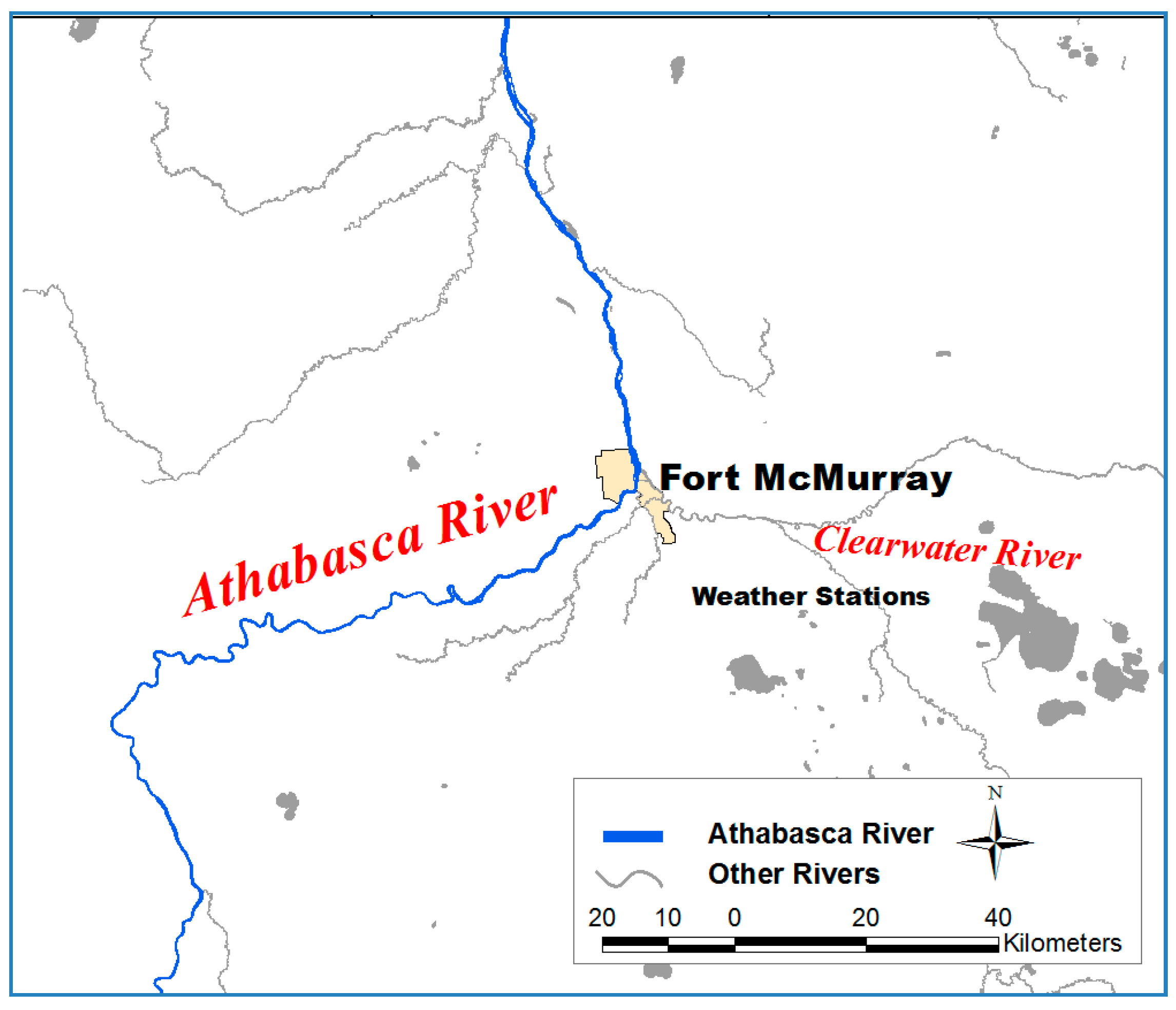
The Athabasca River originates from snow and glacial meltwater in the Columbia Icefields in the southwestern Alberta, Canada [31,32,33,34]. It is the largest, unregulated, northward flowing river in Alberta [35,36]. Fort McMurray is one of the largest towns along the Athabasca River and complicated river channel conditions exist in its vicinity. Upstream of the town, there are a series of major rapids; near the town, the river’s slope decreases by an order of magnitude; in the center of town, the Clearwater River joins the mainstream; and downstream of the town, many sand bars and islands exist in a widened channel. Due to these conditions, there is the frequent potential of ice-related breakup flooding hazard for the Athabasca River at Fort McMurray (Figure 1). Every spring, for northward flowing rivers such as the Athabasca River, due to warming weather, there are increased flow discharges and possibly relative higher temperature water so broken ice sheets are carried down from the upstream to the downstream. Ice jams frequently occur in the nearby reaches due to surges and ice runs from upstream river ice breakup [36,37], which cause back water and related flooding problems [38].

To facilitate the forecasting model development, the historical breakup dates (BDs) for the Athabasca River at Fort McMurray for 1980 to 2015 were collected from the official website of Regional Municipality of Wood Buffalo (http://www.rmwb.ca/). These historical BDs range from early April (Julian day: 100) to early May (123). These BDs are defined as the last date of breakup processes (open channel) at Fort McMurray. Another conventional definition for BDs is the first significant movement date of ice cover (i.e., onset of breakup [39] or the first date of breakup processes [40]). From the perspective of emergency management, the last breakup date is used in this study because it indicates that the town is no longer at ice-related flooding risk.

The potential indicators related to breakup dates were categorized as climate (e.g., air temperature and antecedent precipitation) and river ice (e.g., river flows, water levels, and ice thickness) conditions [41,42,43]. Due to data availability and record length, air temperature was chosen as a potential indicator rather than water temperature. The climate indicators were calculated based on the temperatures and precipitations of two Environment Canada Climate Change stations at Fort McMurray (WMO ID: 71689 and 71585); the missing data gap at the station (71689) were complemented by the other station (71585). The water flows and levels were collected at the Water Survey Canada gauge of Athabasca River below McMurray (Station Number: 07DA001). These indicators were pre-screened as the candidate inputs of the models based on two criteria: availability before breakup and correlation with BDs.

3. Model Development

3.1. Data Preparation

To decrease the different scale effects, all of the data sets were converted into a range of (−1,1) before usage in the models. After calculation, the predicted BDs were transformed back to the original values. Because the river ice breakup dataset was relatively small due to the short period of historical records, a two-step filter-wrapper method was proposed [44,45,46]. Firstly, both the linear correlation coefficients (R) and the mutual information index (MI) between all available input variables and BDs were calculated. A filter method was employed to narrow down the range of these inputs based on the rankings of R and MI. A certain number of inputs with higher rankings were selected as candidate ones. Secondly, based on candidate input variables, a wrapper method was used to determine the optimal combinations of these inputs and inherent parameters of proposed models using a greedy search-based leave-one-out cross validation (LOOCV) method. The average performance of proposed models during LOOCV was evaluated under all possible combinations of inputs and internal parameters. Since the dataset had 36 sets of samples, each model was calibrated using 35 samples and validated through a single sample reserved for each run of LOOCV. The LOOCV ensured all samples be selected once in the validation sets. Generally, since the forecasting performance was of most concern, the model with the best average validation performance was considered the optimal one.

3.2. k-Nearest Neighbor (kNN)

In this study, the inputs of the kNN base models are the climate and river ice condition variables. The output of the kNN model (the predicted BD) is the average of the observed BD values for the k nearest neighbors (feature patterns). The kNN member models can be described as follows:

$$y_{\alpha }=kNN(x_{\alpha })=\frac{1}{k}{\displaystyle \sum _{\beta =1}^k{y}_{\beta }}$$

(1)

$$\beta \in RD(x_{\alpha },x_{\beta },k)$$

(2)

$$x_{\alpha }^{}=[x_{\alpha 1},x_{\alpha 2},\cdots x_{\alpha n}]$$

(3)

where $y_{\alpha }$ is the predicted BD; $x_{\alpha }$ is the corresponding input variable correlated with BD; $y_{\beta }$ is observed BDs of the k nearest neighbors; RD is the ranking between $x_{\alpha }$ and $x_{\beta }$ based on a certain distance function; and $x_{\alpha i}$ is variable i for $x_{\alpha }^{}$(i = 1, 2, …, n). Based on trial and error, two representative distance functions, the Mahalanobis distance (MD) and the Chebychev distance (CD), were employed to calculate the ranking. The MD was chosen since neither the standardization of input variables nor the assignments of weights to variables are required [47]. The definition of MD between a vector ($x_{\alpha }^{}$) and a reference matrix ($X$) is as follows:

$$MD(x_{\alpha }^{},x_{\beta }^{})=\sqrt{\left(x_{\alpha }^{}-\overline{x}\right)COV{(X)}^{-1}{\left(x_{\alpha }^{}-\overline{x}\right)}^T}$$

(4)

$$\overline{x}=[\overline{x_1},\overline{x_2},\cdots \overline{x_n}]$$

(5)

where $\overline{x}$ is the averages for each column of X; $\overline{x_i}$ is the average for column (variable) i of X; $COV{(X)}^{-1}$ is the inverse for the covariance matrix of X [48], and T is the transpose of the vector. The CD between one vector ($x_{\alpha }^{}$) and the other vector ($x_{\beta }^{}$) is defined as follows:

$$CD(x_{\alpha }^{},x_{\beta }^{})={\max }_j\left\{\left|x_{\alpha j}^{}-x_{\beta j}^{}\right|\right\},j=1,2,\cdots ,n$$

(6)

$$x_{\beta }^{}=[x_{\beta 1},x_{\beta 2},\cdots x_{\beta n}]$$

(7)

3.3. Stacking Ensemble Learning

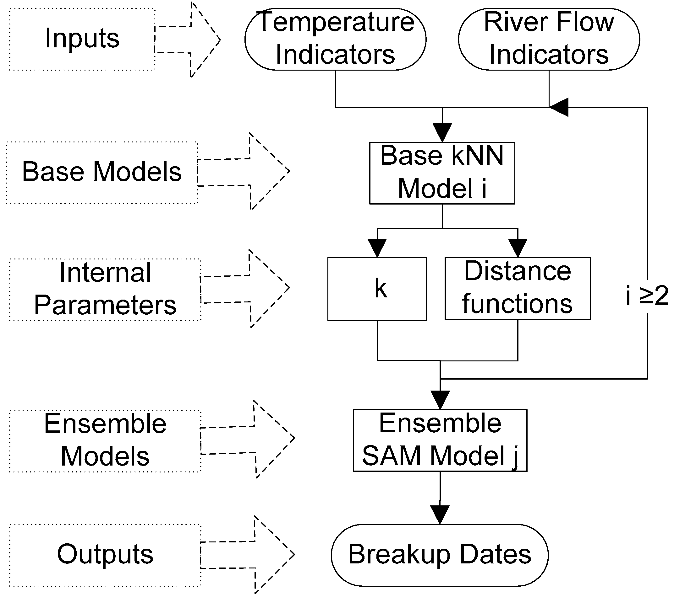
The KSEL for annual river ice breakup dates included base and ensemble models (Figure 2). In terms of its functions, the kNN base models link the BDs with their affecting indicators; the simple average method (SAM) ensemble models describe the relationship between the predicted BDs by each base model and the observed BDs. The SAM can be defined as follows:

$$y_c=\frac{1}{n}{\displaystyle \sum _{i=1}^n{y}_i}$$

(8)

$$\mathrm{var}(y_c-y_o)={\sigma }_c^2=\frac{1}{n}{\sigma }_{i,avg}^2+\frac{n-1}{n}{\sigma }_{i,j,avg}^{}$$

(9)

$${\sigma }_{i,avg}^2=\frac{1}{n}{\displaystyle \sum _{i=1}^n\mathrm{var}(y_i-y)}$$

(10)

$${\sigma }_{i,,j,avg}^{}=\frac{1}{n(n-1)}{\displaystyle \sum _{i=1}^n{\displaystyle \sum _{j=1,j\ne i}^n\mathrm{cov}(y_i-y,y_j-y)}}$$

(11)

where $y_c$ is the output of SAM model, $y_i$ is output of base model i; $y$ is the observed values; n is the number of base models; ${\sigma }_c^2$ is variance of forecasting errors for the SAM; ${\sigma }_{k,avg}^2$ is the average of the error variances (${\sigma }_k^2$) of member models; and ${\sigma }_{i,j,avg}^{}$ is the average of the covariance between each pair of forecasts (${\sigma }_{i,j}^{}$). Based on Equation (4), ${\sigma }_c^2$ is simply equal to ${\sigma }_{i,avg}^2/n$ if the forecast errors of base models are uncorrelated (${\sigma }_{i,j,avg}^{}=0$).

3.4. Model Evaluation

To evaluate the performance of the proposed models, two indices which were the most frequently employed in the forecast models (correlation coefficient (R) and root mean squared error (RMSE)) were selected, [49]. The performance became better with higher R (closer to one) and lower RMSE (closer to zero). The evaluation indices are expressed as follows:

$$R=\frac{{\displaystyle \sum _{j=1}^n(Y_{sj}-\overline{Y_s})(Y_j-\overline{Y})}}{\sqrt{{\displaystyle \sum _{j=1}^n{(Y_{sj}-\overline{Y_s})}^2}}\sqrt{{\displaystyle \sum _{j=1}^n{(Y_j-\overline{Y})}^2}}}$$

(12)

$$RMSE=\sqrt{\frac{{\displaystyle \sum _{j=1}^n{(Y_j-Y_{sj})}^2}}{n-1}}$$

(13)

where n is the sample number in the training or test set, Y_j and Y_sj are the observed and predicted BDs in the jth sample, respectively; and $\overline{Y}$ and $\overline{Y_s}$ are the mean of the observed and predicted BDs. In LOOCV, the training performance of each model was evaluated using the averages of R and RMSE for the training set in m runs. The m is the total number of LOOCV runs. The validation performance of each model was assessed by RSE_avg, (root of average squared errors (SE_i)), which is defined as follows:

$$RootS{E}_{avg}=\sqrt{\frac{{\displaystyle \sum _{i=1}^m{(y_i-y_{si})}^2{}_i}}{m}}$$

(14)

where y_i and y_si are the observed and predicted BD values of the single sample in the validation set for run i of LOOCV.

4. Results analysis

4.1. Climate and River Ice Indicators

Figure 3 shows the 17 candidates climate and river ice indicators, which were obtained based on the filter method. In other words, all of the indicators have higher absolute values of R or MI with BDs. Meanwhile, these indicators are available before April 1 so that they are no later than the earliest breakup date (April 6) in the historical record [50]. These indicators can be categorized as four periods: previous fall (e.g., x₅ and x₇ in last September), during freeze-up (e.g., x₃, x₈, and x₁₁ in last November and x₁₀ and x₁₇ in last December), during middle winter (e.g., x₁ in January), and before breakup (e.g., x₂, x₄, x₆, x₉, and x₁₂ to x₁₆ in March).The dominating negative correlation coefficients of these inputs mean that higher daily temperatures and larger downstream water flows may bring about and be corresponding to earlier BDs. The negative correlation coefficients range from –0.5060 to –0.1705; the positive R values of X₁₁ and X₁₇ 0.0119 and 0.0385, respectively, which are not significant. However, their MI values are relatively higher among temperature indicators, indicating possible nonlinear or interactive correlations. In addition, the MI values of the water flow indicators (3.8429 to 3.5651) are higher than those of temperature indicators (1.8067 to 2.9256) while the difference in R values of both categories are not large. It implies that water flow indicators have more nonlinear correlations with BDs than the temperature indicators.

4.2. kNN-M Base Model

The performance of kNN base models depends on data quality of BDs and indicators, selection of distance functions, combination of indicators, the number (k) of nearest neighbors, and the dataset division strategy. Firstly, the Mahalanobis distance function was employed in the kNN base models (kNN-M). Then the greedy search-based LOOCV method was used to identify the optimal combination of inputs and the internal parameter k. Based on this wrapper method, the k of kNN-M was searched from 2 to 6 and the maximum number of inputs was searched from two to seven.

Table 1. Select kNN models using Mahalanobis distance functions.

Model	Inputs	k	Output	Training		Validation
				Ravg	RMSEavg	RSEavg
kNN-M1	x3, x12	6	-	0.7014	3.697	4.296
kNN-M2	x3, x12, x15	3	y1	0.8513	2.724	3.718
kNN-M3 *	x1, x2, x3, x12	2	y2	0.9187	2.049	3.649
kNN-M4	x1, x2, x6, x10, x15	6	y3	0.7884	3.299	3.800
kNN-M5	x2, x10, x11, x12, x15, x16	3	y4	0.7872	3.254	3.702
kNN-M6	x1, x6, x10, x13, x15, x16, x17	3	y5	0.8345	2.997	3.717

Note: * represents the optimal kNN base model using Mahalanobis distance functions.

lists representative kNN-M models with top performance. All of the kNN-M models had good and diverse performance of training and validation. In terms of validation performance, the kNN-M₃ model with four inputs has the lowest RSE_avg. As for training performance, the kNN-M₃ also had the highest R_avg and the lowest RMSE_avg. Thus, the kNN-M₃ model is considered the optimal one among all the kNN base models using the Mahalanobis distance function.

4.3. kNN-C Base Models

Similarly, the exhaustive-search-based LOOCV method was employed to evaluate the effects of combinations of inputs and k on the performance of kNN base models with the Chebychev distance function (kNN-C). The input numbers were searched from 2 to 8 while the number (k) of nearest neighbors was searched from 2 to 6.

Table 2. Select kNN models using Chebychev distance functions.

Model	Inputs	k	Output	Training		Validation
				Ravg	RMSEavg	RSEavg
KNN-C1	x4, x14	4	-	0.7185	3.595	4.259
KNN-C2	x6, x12, x14	2	y6	0.8951	2.342	3.868
KNN-C3	x1, x2, x3, x12	2	y7	0.8812	2.446	3.524
KNN-C4	x1, x3, x6, x8, x12	2	y8	0.9134	2.134	3.416
KNN-C5 *	x1, x2, x3, x6, x8, x12	2	y9	0.9129	2.125	3.346
KNN-C6	x1, x2, x3, x4, x6, x8, x12	2	y10	0.9127	2.123	3.574

Note: * represents the optimal kNN base model using Chebychev distance functions.

lists representative kNN-C models with top performance. In terms of validation performance, the kNN-C₅ with six inputs has the lowest RSE_avg. As for the training performance, the kNN-C₄ with five inputs has the highest R_avg while the kNN-C₆ with seven inputs has the lowest RMSE_avg. Meanwhile, the kNN-C₅ has very close training performance to the kNN-C₄ and kNN-C₆ in terms of R_avg and RMSE_avg. Since the average validation performance is of most concern, the kNN-C₅ is the optimal one among all kNN-C base models. It is also noted that the optimal kNN-C₅ share four of the same inputs (x₁, x₂, x₃, and x₁₂) with the optimal kNN-M₃.

4.4. kNN-M versus kNN-C Models

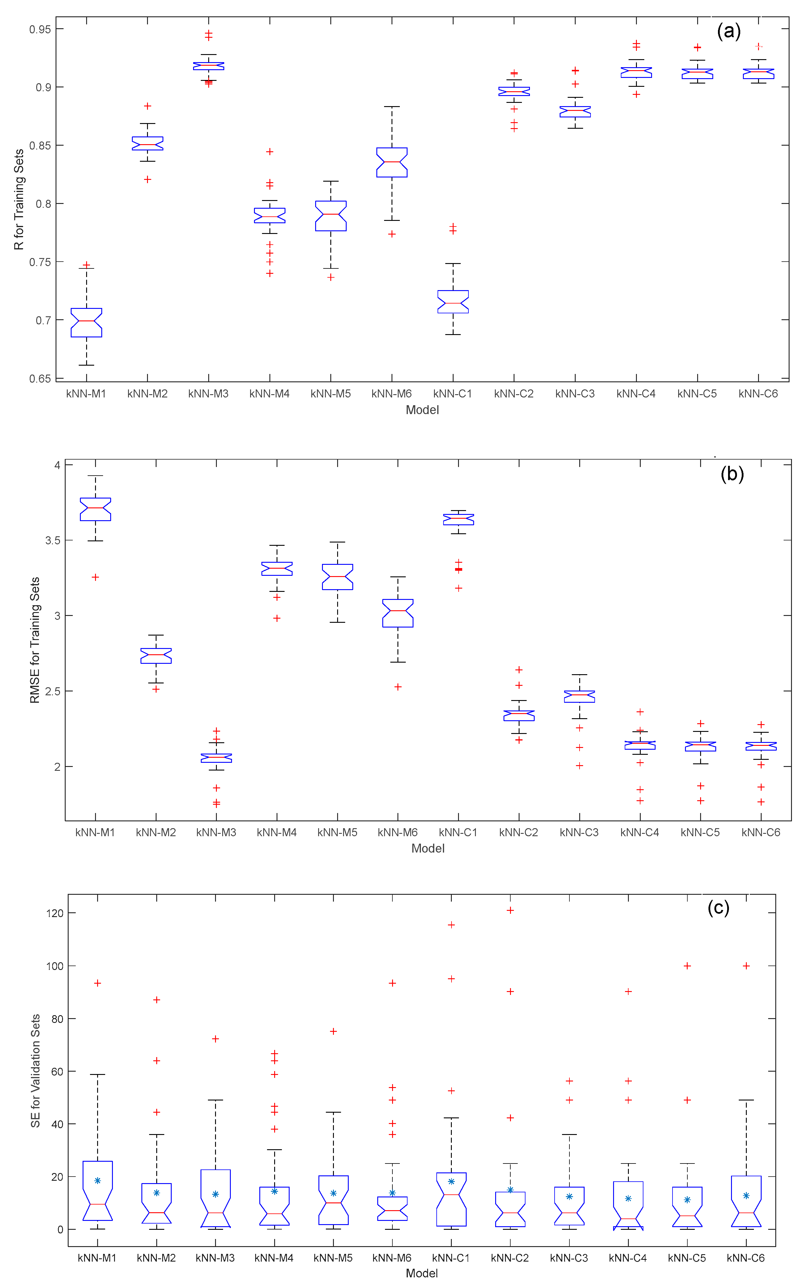
The kNN-M and kNN-C with two to seven inputs (12 kNN base models) were further compared. Figure 4 shows a comparison of their performance index distributions. For training sets, the R distributions of kNN-C models except kNN-C₁ are generally higher and their RMSE distributions are lower than those of kNN-M models; in other words, when the number of inputs are larger than two, the performance of the kNN-C models becomes better than those of the kNN-M. The R and RMSE distributions of kNN-M models appear to have diverse positions. The index distributions of the kNN-M₂ with two inputs are the worst among kNN-M models while those of kNN-M₃ with three inputs are in the optimal position. As for validation sets, the SE distributions for the kNN-C models except kNN-C₁ are generally lower and their RMSE distributions between the 25th and 75th percentiles become narrower than those of the kNN-M models. Among the kNN-C models, although the kNN-C₅ has the lowest mean SE values, the extreme SE values of kNN-C₃ and the median SE values of kNN-C₄ are the lowest; among the kNN-M models, although the kNN-M₃ has the lowest mean SE values, it has relatively wider distributions between the 25th and 75th percentiles than most of kNN-M models. Meanwhile, the extreme SE values of the kNN-M₄ are slightly lower than those of the kNN-M₃. Based on this comparison of the diverse performance, ten kNN based models (kNN-M₂ to kNN-M₆ and kNN-C₂ to kNN-C₆) were chosen as the representative base models for further combination in the ensemble models.

4.5. kNN Ensemble Models Using Single-Type Distance Functions

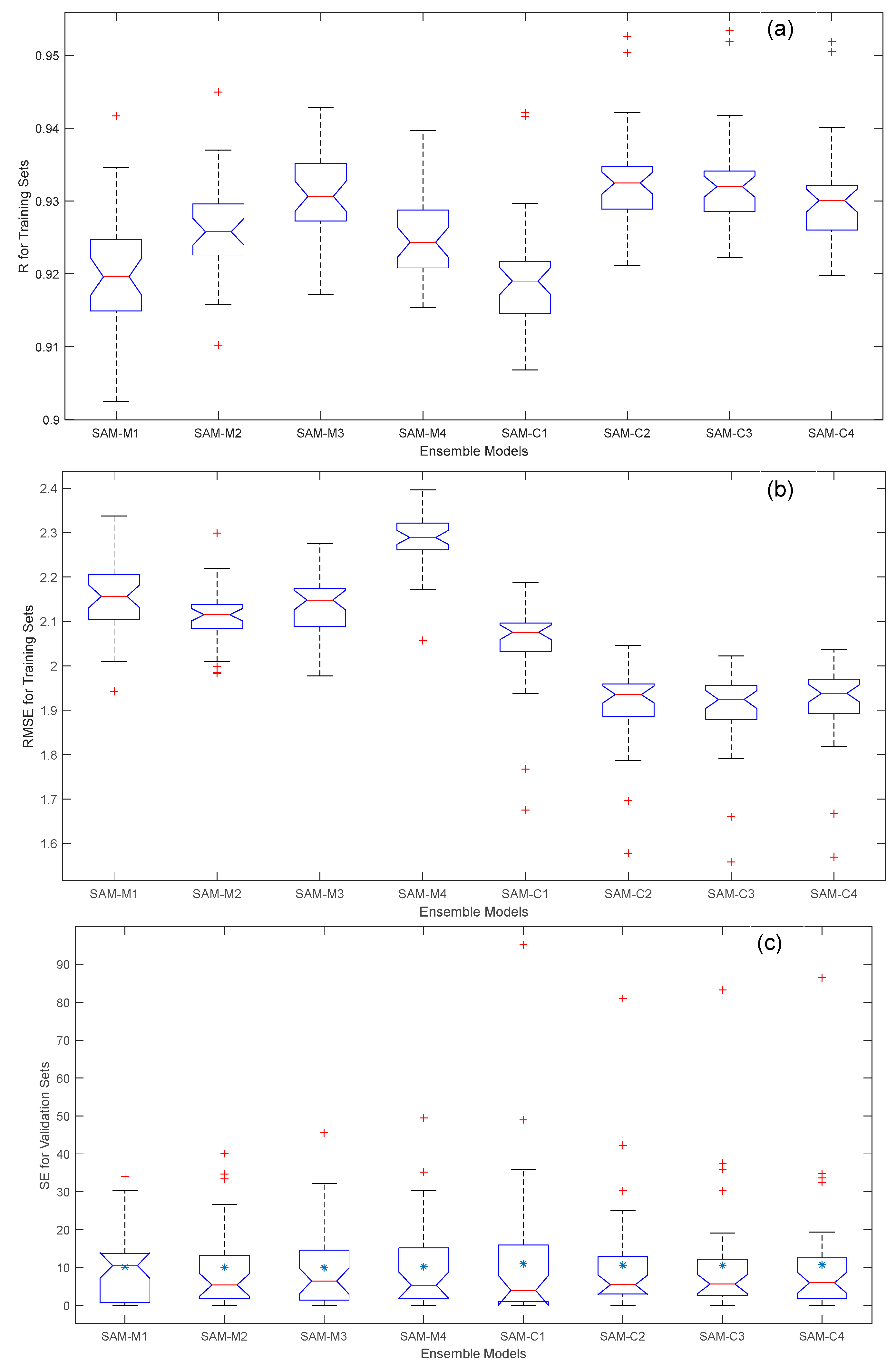
To evaluate the performance of ensemble kNN models using single-type distance functions, the outputs of the selected kNN-M models (kNN-M₂ to kNN-M₆) as well as the selected kNN-C models (kNN-C₂ to kNN-C₆) were combined as inputs for the SAM-M and SAM-C ensemble models, respectively. Both SAM-M and SAM-C with all possible combinations of inputs (i.e., the outputs of kNN-M or kNN-C) were evaluated through the exhaustive-search-based LOOCV method. The numbers of base models were searched from two to five. The SAM-M and SAM-C models of top performance are listed in

Table 3. Select kNN-based stacking ensemble models using single-type distance functions.

Model	Inputs	Distance Function	Training		Validation
			Ravg	RMSEavg	RSEavg
SAM-M1	y2, y4	Mahalanobis	0.9201	2.154	3.181
SAM-M2	y1, y2, y4	Mahalanobis	0.9262	2.112	3.170
SAM-M3 *	y1, y2, y4, y5	Mahalanobis	0.9308	2.136	3.161
SAM-M4	y1, y2, y3, y4, y5	Mahalanobis	0.9249	2.283	3.202
SAM-C1	y8, y9	Chebychev	0.9191	2.054	3.319
SAM-C2	y6, y7, y9	Chebychev	0.9328	1.913	3.262
SAM-C3 *	y6, y7, y8, y9	Chebychev	0.9326	1.903	3.247
SAM-C4	y6, y7, y8, y9, y10	Chebychev	0.9306	1.918	3.282

Note: * represents the optimal ensemble model of each type.

. It can be seen that compared with the kNN base models, both SAM-M and SAM-C improved upon the corresponding kNN-M and kNN-C. Meanwhile, the training performance of the SAM-C models was slightly better than those of the SAM-M models while the validation performance of the former was slightly worse than those of the latter. Especially, the R_avg values of the SAM-C models (0.9328 to 0.9191) were slightly higher than or almost equal to those of the SAM-M models (0. 9308 to 0.9201), the RMSE_avg values of the former (1.903 to 2.054) were lower than the latter (2.112 to 2.283). However, the former had higher RSE_avg values (3.247 to 3.319) than the latter (3.161 to 3.202). Overall, the performance differences of all these SAM models were relatively small. Among them, the SAM-M₃ and SAM-C₃ models are the optimal SAM ensemble models with each type of distance function. The distributions of performance indices for the selected kNN-M and kNN-C were further compared in Figure 5. The distribution locations of training performance indices (R and RMSE) for the kNN-M were generally higher and lower than those of the kNN-C, respectively. The distributions of validation performance indices (SE) for the former were generally lower than those of the latter; this was especially true for the extreme value forecasting.

4.6. kNN Ensemble Models Using Multiple-Type Distance Functions

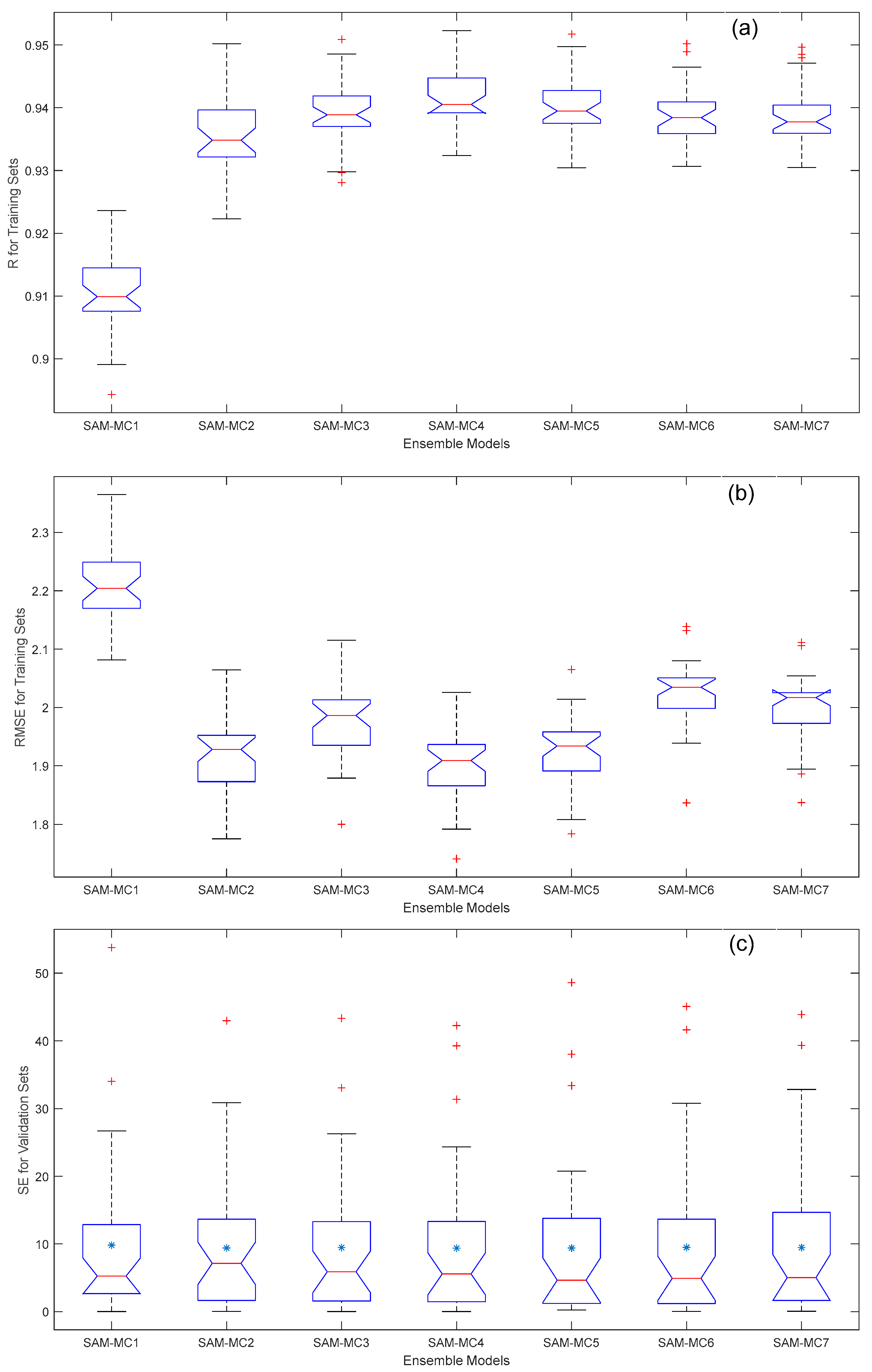
Similarly, the performance of ensemble kNN models using multiple-type distance functions (kNN-MC) was evaluated based on the outputs of the ten selected kNN-M and kNN-C models (y₁ to y₁₀). The possible combination numbers of base models were searched from two to eight through the exhaustive-search-based LOOCV method. The SAM-MC models with top performance are listed in

Table 4. Select kNN-based stacking ensemble models using multiple-type distance functions.

Model	Inputs	Number of Distance Functions		Training		Validation
		Mahalanobis	Chebychev	Ravg	RMSEavg	RSEavg
SAM-MC1	y4, y9	1	1	0.9105	2.205	3.131
SAM-MC2	y2, y4, y9	2	1	0.9357	1.918	3.065
SAM-MC3	y2, y4, y5, y9	3	1	0.9392	1.977	3.075
SAM-MC4 *	y2, y4, y5, y8, y9	3	2	0.9416	1.900	3.062
SAM-MC5	y1, y2, y4, y5, y8, y9	4	2	0.9401	1.925	3.063
SAM-MC6	y1, y2, y3, y4, y5, y8, y9	5	2	0.9386	1.924	3.071
SAM-MC7	y1, y2, y3, y4, y5, y7, y8, y9	5	3	0.9385	1.999	3.077

Note: * represents the optimal ensemble model of all models.

. It is noted that the validation performance of these SAM-MC models was substantially better and better than those of kNN base and SAM-M or SAM-C models, respectively. Except for the SAM-MC₁ model, the training performance of the other SAM-MC models was better than those of kNN base and SAM-M as well as slightly better than those of SAM-C models, respectively. Especially, the R_avg (0.9357 to 0.9416), RMSE_avg (1.900 to 1.999), and RSE_avg (3.062 to 3.077) values of the SAM-MC₂ to SAM-MC₇ models were respectively higher, lower and lower than those of almost all kNN base and SAM-M (or SAM-C) models. Overall the SAM-MC₄ with the lowest RSE_avg (3.062), the highest R_avg (0.9416), and the lowest RMSE_avg (1.900) is the optimal kNN ensemble model. The distributions of performance indices for the selected kNN-MC were further compared in Figure 6. The distributions of training performance indices for most of the kNN-MC models except the kNN-MC₁ were generally in good positions. The distributions of their validation performance indices for these kNN-MC models were also in similar good positions. It implies the robustness of the proposed KSEL method.

4.7. Optimal Ensemble kNN Model

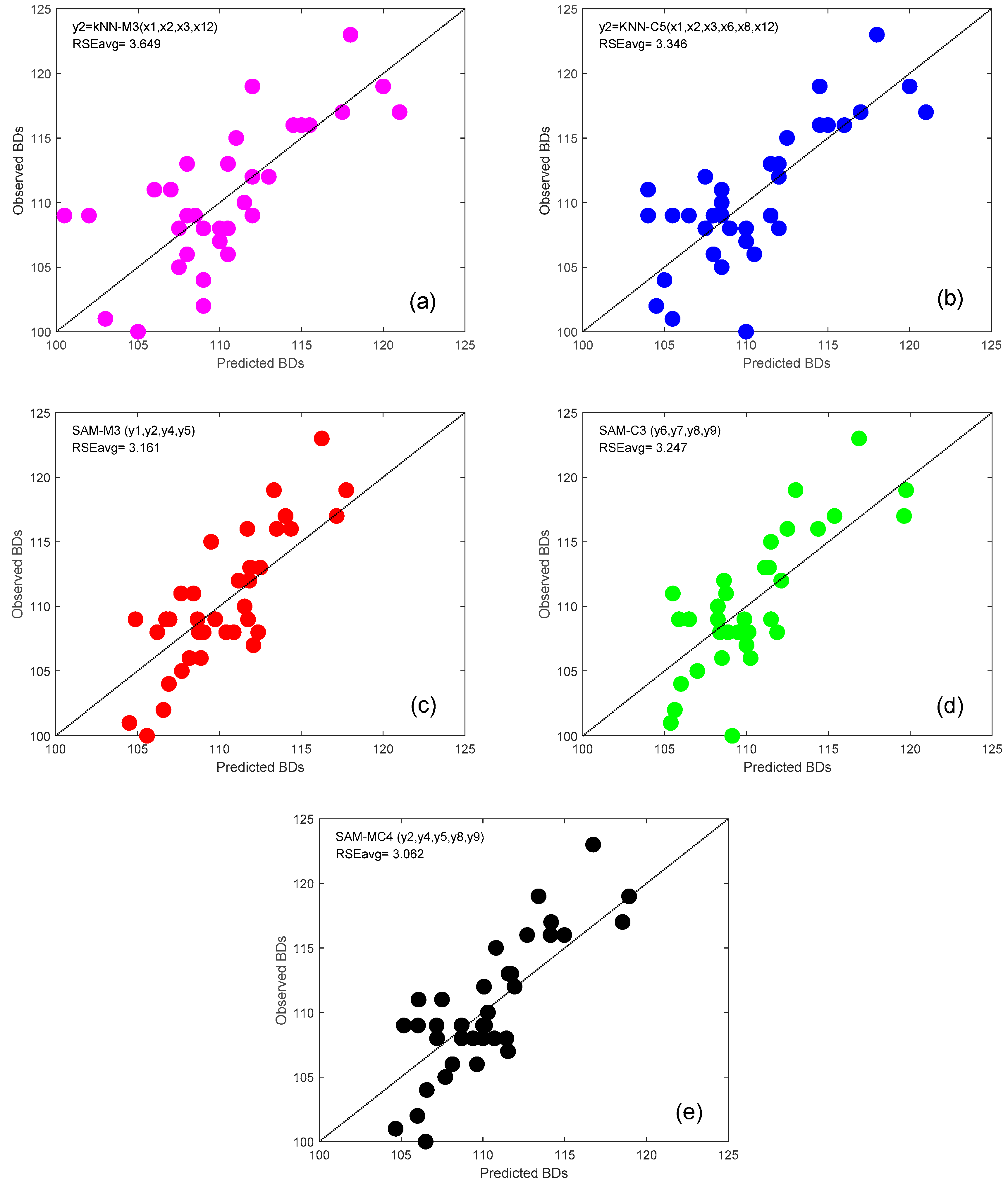
Figure 7 shows the further comparison of the validation performance in each run of the LOOCV method among the optimal kNN ensemble and base models. Compared with the optimal kNN base model, the SAM-MC₄ has obviously closer distances between the data dots and the equal-value line, which indicates improved performance compared to kNN-M₃ and kNN-C₅. Compared with the optimal kNN ensemble model with the single-type distance functions, deviations of the SAM-MC₄ model decrease slightly from the equal-value lines than SAM-M₃ and SAM-C₃. These improvements are especially true for the lower and middle ranges of the BD. In terms of RSE_avg values, the SAM-MC₄ improves upon SAM-M₃, SAM-C₃, kNN-M_3, and kNN-C₅ by 3.13%, 5.70%, 16.09%, and 8.49%, respectively.

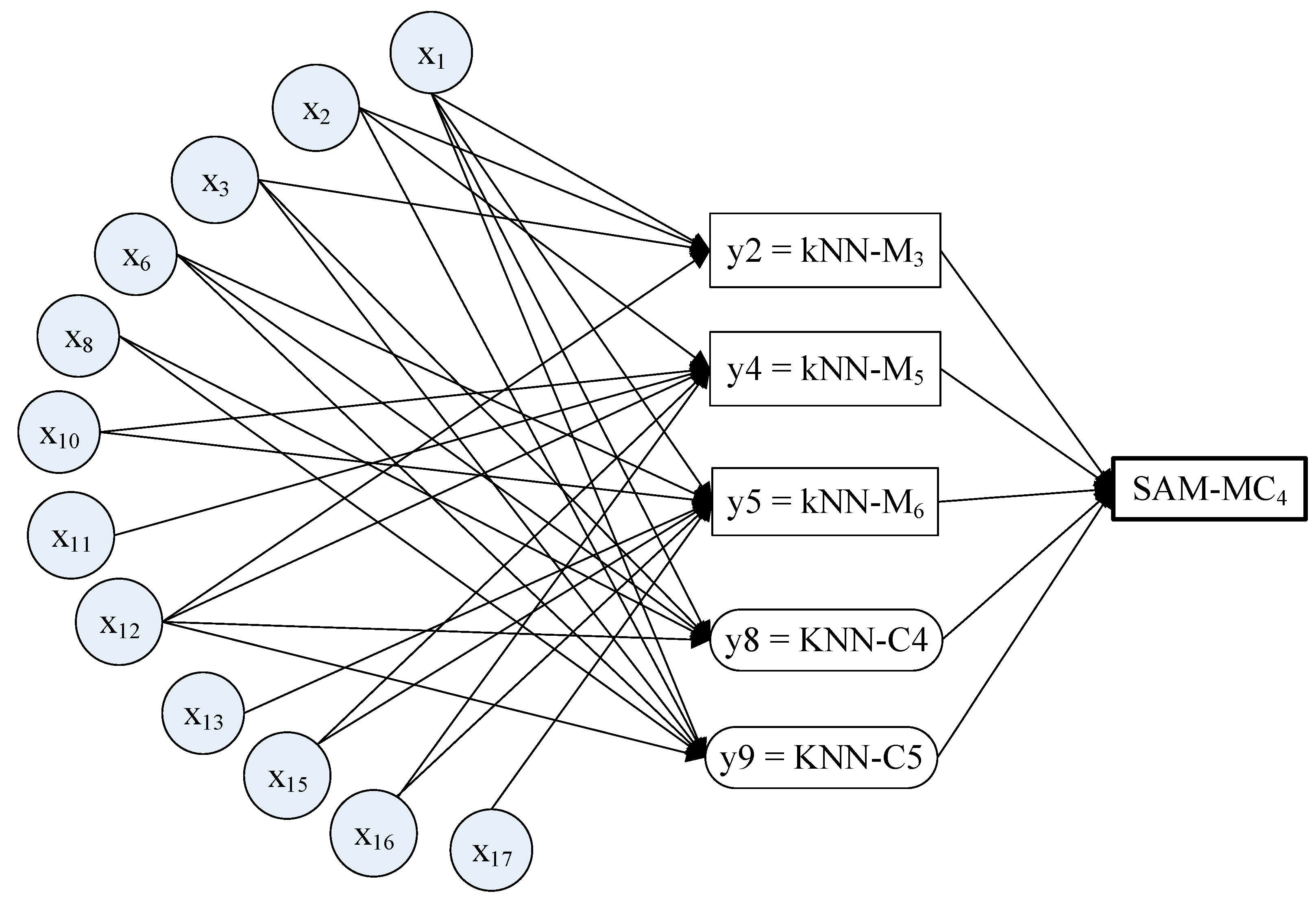
Figure 8 illustrates the structure of the SAM-MC₄, which combines the outputs from five base models (y₂, y₄₅, y₅, y₈ and y₉). These base models have totally twelve inputs. All of the inputs can be categorized as temperature and water flow conditions just before breakup (e.g., x₂, x₆, x₁₂, x₁₃, x_15, and x₁₆ in March), during freeze-up (e.g., x₃, x₈, and x₁₁ in last November and x₁₀ and x₁₇ in last December) and during middle winter (e.g., x₁ in January). From the data-driven perspective, the inclusion of certain inputs as well as their numbers in the optimal models can reveal some hints of potential mechanism on ice breakup. The twelve inputs of the optimal SAM-MC₄ may indicate that the breakup timing is mainly linked with temperature and water flow conditions before breakup. However, the breakup timing is also related to conditions during and just after freeze-up due to the upstream and downstream relations. Previous studies have reported the breakup flooding maybe affected by a combination of conditions during freeze-up and breakup [39,51].

5. Discussions

Many numerical methods have been applied to simulating river ice breakup processes [11,12] or to forecasting breakup dates [52,53]. When numerical methods are employed, it is usually critical for modelling breakup dates through distinguishing between thermal and mechanical breakup. In comparison, the proposed kNN-based stacking ensemble learning (KSEL) method is able to handle both breakup types simultaneously. This is because the kNN avoids quantification of complex river ice breakup mechanisms described by scarce data. As long as different types of relations between indicators and breakup dates exist in the historical data, the KNN can be implemented based on the similarity with previous relations, which is quantified using the selected distance functions. Thus, the KSEL is especially useful for the unchanged climate conditions. When new data are available under climate change conditions, these new data can be easily added into the training dataset so that the KSEL can be adjusted accordingly.

Some data-driven methods have been applied to simulating river ice breakup processes [54,55,56]. In particular, the Bayesian regularization back-propagation artificial neural network (BRANN), adaptive neuro fuzzy inference systems (ANFIS), the classification and regression tree (CART), and M5 models as well as their ensembles have all been proposed for forecasting breakup dates [57,58]. Compared with these models, the kNN has the simplest calculation strategy with comparable computing performance. In addition, if new data are available, the training stage for the kNN is minimal while some of other machine learning models may need more training time for parameter calibration. Nevertheless, it was reported that the kNN cannot predict well the highest and lowest extreme values since the output is the average of the k nearest neighbors [27].

Besides the advantage of kNN, the performance of the proposed KSEL has been improved over each optimal kNN base model because of the ensemble structure. The multiple distance functions employed in multiple kNN base models do bring diversity to the ensemble framework. The stacking ensemble learning is a simple but effective manner to combine kNN models since other ensemble methods, such as boosting and bagging, have limited ability to improve kNN performance. To further bring diversity to the KSEL, different types of machine learning methods with different structures and performance can be introduced [59,60,61]. Combining other machine learning methods with the kNN may further improve the overall performance of the ensemble framework [62]. The promising application of the ensemble framework to various river ice forecasting problems is expected.

6. Conclusions

A kNN-based stacking ensemble learning (KSEL) method was developed and applied to forecasting annual river ice breakup dates (BDs) for the Athabasca River at Fort McMurray. The kNN base models with diverse inputs and distance functions were developed. The outputs of kNN base models with single or multiple types of distance functions were further combined through the simple average methods. The historical BDs and corresponding climate and river conditions in 1980–2015 were collected to facilitate the model development. The performance of these models was examined using the LOOCV. The major findings are as follows: (1) the kNN models are able to build nonlinear relationships between indicators and BDs with different performance. For the investigated river ice data, the kNN with the Chebychev distance functions (kNN-C) generally outperformed the one with the Mahalanobis distance functions (kNN-M) in terms of validation and training performance; (2) based on the simple average methods, the kNN ensemble models using single-type distance functions (SAM-M and SAM-C) outperformed the corresponding the kNN base models. The ensemble kNN models using multiple-type distance functions (SAM-MC) further improved the overall performance. In terms of RSE_avg values, the optimal SAM-MC improved upon the optimal kNN-M, kNN-C, SAM-M, and SAM-C models by 3.13%, 5.70%, 16.09%, and 8.49%, respectively; (3) from the data-driven perspective, the twelve inputs of the optimal SAM-MC may indicate that the breakup timing is mainly linked with temperature and water flow conditions before breakup as well as during and just after freeze up; and (4) this study, for the first time, applied the KSEL methods to forecasting of river ice breakup timing. Combining diverse abilities of machine learning models through stacking ensemble learning appears promising for river ice forecasting problems.

References

- Prowse, T.; Shrestha, R.; Bonsal, B.; Dibike, Y. Changing spring air-temperature gradients along large northern rivers: Implications for severity of river-ice floods. Geophys. Res. Lett. 2010, 37, L19706. [Google Scholar] [CrossRef]
- She, Y.; Andrishak, R.; Hicks, F.; Morse, B.; Stander, E.; Krath, C.; Keller, D.; Abarca, N.; Nolin, S.; Tanekou, F.; et al. Athabasca River ice jam formation and release events in 2006 and 2007. Cold Reg. Sci. Technol. 2009, 55, 249–261. [Google Scholar] [CrossRef]
- Hicks, F.; Beltaos, S. River ice. In Cold Region. Atmospheric and Hydrologic Studies. The Mackenzie GEWEX Experience; Woo, M.-k., Ed.; Springer: New York, NY, USA, 2007; pp. 281–305. [Google Scholar]
- Hicks, F. An overview of river ice problems: CRIPE07 guest editorial. Cold Reg. Sci. Technol. 2009, 55, 175–185. [Google Scholar] [CrossRef]
- Beltaos, S.; Burrell, B. Hydrotechnical advances in Canadian river ice science and engineering during the past 35 years. Can. J. Civ. Eng. 2015, 42, 583–591. [Google Scholar] [CrossRef]
- Beltaos, S.; Tang, P.; Rowsell, R. Ice jam modelling and field data collection for flood forecasting in the Saint John River. Can. Hydrol. Process. 2012, 26, 2535–2545. [Google Scholar]
- Chen, D.L.; Liu, J.F.; Zhang, L.N. Application of Statistical Forecast Models on Ice Conditions in the Ningxia-Inner Mongolia Reach of the Yellow River. In Ice Research for a Sustainable Environment; Li, Z., Lu, P., Eds.; Dalian University of Technology: Dalian, China, 2012; pp. 443–454. [Google Scholar]
- Hu, J.; Liu, L.; Huang, Z.; You, Y.; Rao, S. Ice breakup date forecast with hybrid artificial neural networks. In Proceedings of the 2008 Fourth International Conference on Natural Computation, Jinan, China, 18–20 October 2008; IEEE: Piscataway, NJ, USA, 2008. [Google Scholar]
- Zhang, B.S.; Ji, H.L.; Xu, J.; Zhang, A.D.; Bian, X.J. Ice Forecasting Model Based on the Variable Fuzzy Synthetic Analysis. In Ice Research for a Sustainable Environment; Li, Z., Lu, P., Eds.; Dalian University of Technology: Dalian, China, 2012; pp. 467–474. [Google Scholar]
- Zhao, L.; Hicks, F.E.; Robinson Fayek, A. Applicability of multilayer feed-forward neural networks to model the onset of river breakup. Cold Reg. Sci. Technol. 2012, 70, 32–42. [Google Scholar] [CrossRef]
- Knack, I.M.; Shen, H.T. A numerical model study on Saint John River ice breakup. Can. J. Civ. Eng. 2018, 45, 817–826. [Google Scholar] [CrossRef]
- Shen, H.T. Mathematical modeling of river ice processes. Cold Reg. Sci. Technol. 2010, 62, 3–13. [Google Scholar] [CrossRef]
- Karlsson, M.; Yakowitz, S. Nearest-Neighbor Methods for Nonparametric Rainfall-Runoff Forecasting. Water Resour. Res. 1987, 23, 1300–1308. [Google Scholar] [CrossRef]
- Galeati, G. A Comparison of Parametric and Non-Parametric Methods for Runoff Forecasting. Hydrol. Sci. J. -J. Des Sci. Hydrol. 1990, 35, 79–94. [Google Scholar] [CrossRef]
- Kember, G.; Flower, A.C.; Holubeshen, J. Forecasting River Flow Using Nonlinear Dynamics. Stoch. Hydrol. Hydraul. 1993, 7, 205–212. [Google Scholar] [CrossRef]
- Shamseldin, A.Y.; Oconnor, K.M. A nearest neighbour linear perturbation model for river flow forecasting. J. Hydrol. 1996, 179, 353–375. [Google Scholar] [CrossRef]
- Makungo, R.; Odiyo, J.O.; Ndiritu, J.G.; Mwaka, B. Rainfall-runoff modelling approach for ungauged catchments: A case study of Nzhelele River sub-quaternary catchment. Phys. Chem. Earth. 2010, 35, 596–607. [Google Scholar] [CrossRef]
- St-Hilaire, A.; Ouarda, T.; Bargaoui, Z.; Daigle, A.; Bilodeau, L. Daily river water temperature forecast model with a k-nearest neighbour approach. Hydrol. Process. 2012, 26, 1302–1310. [Google Scholar] [CrossRef]
- Caldwell, R.J.; Gangopadhyay, S.; Bountry, J.; Lai, Y.; Elsner, M.M. Statistical modeling of daily and subdaily stream temperatures: Application to the Methow River Basin, Washington. Water Resour. Res. 2013, 49, 4346–4361. [Google Scholar] [CrossRef]
- Saghafian, B.; Anvari, S.; Morid, S. Effect of Southern Oscillation Index and spatially distributed climate data on improving the accuracy of Artificial Neural Network, Adaptive Neuro-Fuzzy Inference System and K-Nearest Neighbour streamflow forecasting models. Expert Syst. 2013, 30, 367–380. [Google Scholar] [CrossRef]
- Gharun, M.; Azmi, M.; Adams, M.A. Short-Term Forecasting of Water Yield from Forested Catchments after Bushfire: A Case Study from Southeast Australia. Water 2015, 7, 599–614. [Google Scholar] [CrossRef]
- Kan, G.Y.; Yao, C.; Li, Q.L.; Li, Z.J.; Yu, Z.B.; Liu, Z.Y.; Ding, L.Q.; He, X.Y.; Liang, K. Improving event-based rainfall-runoff simulation using an ensemble artificial neural network based hybrid data-driven model. Stoch. Environ. Res. Risk Assess. 2015, 29, 1345–1370. [Google Scholar] [CrossRef]
- Sharifazari, S.; Araghinejad, S. Development of a Nonparametric Model for Multivariate Hydrological Monthly Series Simulation Considering Climate Change Impacts. Water Resour. Manag. 2015, 29, 5309–5322. [Google Scholar] [CrossRef]
- Wei, C.C. Comparing lazy and eager learning models for water level forecasting in river-reservoir basins of inundation regions. Environ. Model. Softw. 2015, 63, 137–155. [Google Scholar] [CrossRef]
- Lu, Y.; Qin, X.S.; Mandapaka, P.V. A combined weather generator and K-nearest-neighbour approach for assessing climate change impact on regional rainfall extremes. Int. J. Climatol. 2015, 35, 4493–4508. [Google Scholar] [CrossRef]
- Lu, Y.; Qin, X.S. A coupled K-nearest neighbour and Bayesian neural network model for daily rainfall downscaling. Int. J. Climatol. 2014, 34, 3221–3236. [Google Scholar] [CrossRef]
- Sun, W.; Trevor, B. Combining k-nearest-neighbor models for annual peak breakup flow forecasting. Cold Reg. Sci. Technol. 2017, 143, 59–69. [Google Scholar] [CrossRef]
- Bay, S.D. Combining Nearest Neighbor Classifiers Through Multiple Feature Subsets; Citeseer, ICML: Long Beach, CA, USA, 1998. [Google Scholar]
- Bao, Y.G.; Ishii, N.; Du, X.Y. Combining multiple k-nearest neighbor classifiers using different distance functions. In Proceedings of the 5th International Conference Intelligent Daa Engineering and Automated Learning Ideal 2004, Exeter, UK, 25–27 August 2004; Yang, Z.R., Everson, R., Yin, H., Eds.; Springer: Berlin, Germany, 2004; pp. 634–641. [Google Scholar]
- Tahir, M.A.; Smith, J. Creating diverse nearest-neighbour ensembles using simultaneous metaheuristic feature selection. Pattern Recognit. Lett. 2010, 31, 1470–1480. [Google Scholar] [CrossRef] [Green Version]
- Peters, D.L.; Monk, W.A.; Baird, D.J. Cold-regions Hydrological Indicators of Change (CHIC) for ecological flow needs assessment. Hydrol. Sci. J. -J. Des Sci. Hydrol. 2014, 59, 502–516. [Google Scholar] [CrossRef]
- Peters, D.L.; Atkinson, D.; Monk, W.A.; Tenenbaum, D.E.; Baird, D.J. A multi-scale hydroclimatic analysis of runoff generation in the Athabasca River, western Canada. Hydrol. Process. 2013, 27, 1915–1934. [Google Scholar] [CrossRef]
- Andrishak, R.; Abarca, J.N.; Wojtowicz, A.; Hicks, F. Freeze-up study on the lower Athabasca River (Alberta, Canada). Presented at the 19 IAHR International Symposium on Ice: Using New Technology to Understand Water-Ice Interaction, Vancouver, BC, Canada, 6–11 July 2008. [Google Scholar]
- Andrishak, R.; Hicks, F. Ice effects on flow distributions within the Athabasca Delta, Canada. River Res. Appl. 2011, 27, 1149–1158. [Google Scholar] [CrossRef]
- Sun, W.; Trevor, B.; Kovachis, N. Athabasca River Ice Observations 2014–2015 (Annual Report); Alberta Environment and Parks: Edmonton, AB, Canada, 2015. [Google Scholar]
- Kowalczyk, T.; Hicks, F. Observations of dynamic ice jam release on the Athabasca River at Fort McMurray, AB. Presented at the 12th Workshop on River Ice, Edmonton, AB, Canada, 19–20 June 2003. [Google Scholar]
- She, Y.; Hicks, F. Modeling ice jam release waves with consideration for ice effects. Cold Reg. Sci. Technol. 2006, 45, 137–147. [Google Scholar] [CrossRef]
- Sun, W.; Trevor, B. A Comparison of Fuzzy Logic Models for Breakup Forecasting of the Athabasca River, in CGU HS Committee on River Ice Processes and the Environment. Presented at the 18th Workshop on the Hydraulics of Ice Covered Rivers, Quebec City, QC, Canada, 18–21 August 2015. [Google Scholar]
- Beltaos, S. River Ice Breakup; Water Resources Publications, LLC: Highlands Ranch, CO, USA, 2008. [Google Scholar]
- Zhao, L.; Hicks, F.; Fayek, A.R.; Kovachis, N. Forecasting the Onset of Breakup using Artificial Neural Networks. Presented at the 20th IAHR International Symposium on Ice, Lahti, Finland, 14–18 June 2010. [Google Scholar]
- Bieniek, P.A.; Bhatt, U.S.; Rundquist, L.A.; Lindsey, S.D.; Zhang, X.; Thoman, R.L. Large-scale climate controls of interior Alaska river ice breakup. J. Clim. 2011, 24, 286–297. [Google Scholar] [CrossRef] [Green Version]
- Cooley, S.W.; Pavelsky, T.M. Spatial and temporal patterns in Arctic river ice breakup revealed by automated ice detection from MODIS imagery. Remote. Sens. Environ. 2016, 175, 310–322. [Google Scholar] [CrossRef]
- Sun, W.; Shi, Q.; Huang, Y.; Lv, Y. Ensemble Learning Enhanced Stepwise Cluster Analysis for River Ice Breakup Date Forecasting. J. Environ. Inf. Lett. 2019, 1, 37–47. [Google Scholar] [CrossRef]
- Vergara, J.R.; Estévez, A. A review of feature selection methods based on mutual information. Neural Comput. Appl. 2014, 24, 175–186. [Google Scholar] [CrossRef]
- May, R.; Dandy, G.; Maier, H. Review of input variable selection methods for artificial neural networks. In Artificial Neural Networks—Methodological Advances and Biomedical Applications; INTECH Open Access: London, UK, 2011. [Google Scholar]
- Maier, H.R.; Jain, A.; Dandy, G.C.; Sudheer, K.P. Methods used for the development of neural networks for the prediction of water resource variables in river systems: Current status and future directions. Environ. Model. Softw. 2010, 25, 891–909. [Google Scholar] [CrossRef]
- Yates, D.; Gangopadhyay, S.; Rajagopalan, B.; Strzepek, K. A technique for generating regional climate scenarios using a nearest-neighbor algorithm. Water Resour. Res. 2003, 39, 1199. [Google Scholar] [CrossRef] [Green Version]
- De Maesschalck, R.; Jouan-Rimbaud, D.; Massart, D.L. The mahalanobis distance. Chemom. Intell. Lab. Syst. 2000, 50, 1–18. [Google Scholar] [CrossRef]
- Oyebode, O.; Otieno, F.; Adeyemo, J. Review of Three Data-Driven Modelling Techniques for Hydrological Modelling and Forecasting. Fresenius Environ. Bull. 2014, 23, 1443–1454. [Google Scholar]
- Mahabir, C.L. River Ice Breakup Forecasting with Fuzzy and Neuro-fuzzy Models. Ph.D. Thesis, University of Alberta, Edmonton, AB, Canada, September 2007. [Google Scholar]
- Lagadec, A.; Boucher, E.; Germain, D. Tree ring analysis of hydro-climatic thresholds that trigger ice jams on the Mistassini River, Quebec. Hydrol. Process. 2015, 29, 4880–4890. [Google Scholar] [CrossRef]
- Wang, J.; He, L.; Chen, P.P.; Sui, J.Y. Numerical simulation of mechanical breakup of river ice-cover. J. Hydrodyn. 2013, 25, 415–421. [Google Scholar] [CrossRef]
- Ma, X.Y.; Fukushima, Y. A numerical model of the river freezing process and its application to the Lena River. Hydrol. Process. 2002, 16, 2131–2140. [Google Scholar] [CrossRef]
- Wang, T.; Yang, K.L.; Guo, Y.X. Application of artificial neural networks to forecasting ice conditions of the Yellow River in the Inner Mongolia reach. J. Hydrol. Eng. 2008, 13, 811–816. [Google Scholar]
- Zhao, L.; Hicks, F.E.A.; Robinson, F. Long lead forecasting of spring peak runoff using Mamdani-type fuzzy logic systems at Hay River, NWT. Can. J. Civ. Eng. 2015, 42, 665–674. [Google Scholar] [CrossRef]
- Lindenschmidt, K.E.; Das, A.; Rokaya, P.; Chu, T.A. Ice-jam flood risk assessment and mapping. Hydrol. Process. 2016, 30, 3754–3769. [Google Scholar] [CrossRef]
- Sun, W. River ice breakup timing prediction through stacking multi-type model trees. Sci. Total Environ. 2018, 644, 1190–1200. [Google Scholar] [CrossRef] [PubMed]
- Sun, W.; Trevor, B. A stacking ensemble learning framework for annual river ice breakup dates. J. Hydrol. 2018, 561, 636–650. [Google Scholar] [CrossRef]
- Wu, W.; Liu, H.B. Assessment of monthly solar radiation estimates using support vector machines and air temperatures. Int. J. Climatol. 2012, 32, 274–285. [Google Scholar] [CrossRef]
- Teegavarapu, R.S.V.; Aly, A.; Pathak, C.S.; Ahlquist, J.; Fuelberg, H.; Hood, J. Infilling missing precipitation records using variants of spatial interpolation and data-driven methods: Use of optimal weighting parameters and nearest neighbour-based corrections. Int. J. Climatol. 2018, 38, 776–793. [Google Scholar] [CrossRef]
- Kisi, O.; Sanikhani, H. Modelling long-term monthly temperatures by several data-driven methods using geographical inputs. Int. J. Climatol. 2015, 35, 3834–3846. [Google Scholar] [CrossRef]
- Sun, W.; Trevor, B. Multiple Model Combination Methods for Annual Maximum Water Level Prediction during River Ice Breakup. Hydrol. Process. 2018, 32. [Google Scholar] [CrossRef]
Figure 1.
The Athabasca River at Fort McMurray in Alberta, Canada.
Figure 2.
Framework of k-nearest neighbor (kNN)-based stacking ensemble learning (KSEL).
Figure 3.
Relations between indicators and breakup dates. (a) Correlation coefficients. (b) Mutual information indices
Figure 4.
Performance of selected kNN models. (a) R for training sets. (b) RMSE for training sets. (c) SE for validation sets.
Figure 5.
Performance of selected kNN-based stacking ensemble learning models using single-type distance functions. (a) R for training sets. (b) RMSE for training sets. (c) SE for validation sets.
Figure 6.
Performance of selected kNN-based stacking ensemble learning models using multiple-type distance functions. (a) R for training sets. (b) RMSE for training sets. (c) SE for validation sets.
Figure 7.
Validation performance of optimal base and ensemble kNN models. (a) kNN-M3. (b) KNN-C5. (c) SAM-M3. (d) SAM-C3. (e) SAM-MC4.
Figure 8.
Structure of optimal kNN-based stacking ensemble learning model.