Application of Open Source Electronics for Measurements of Surface Water Properties in an Estuary: A Case Study of River Jadro, Croatia

 , , , and
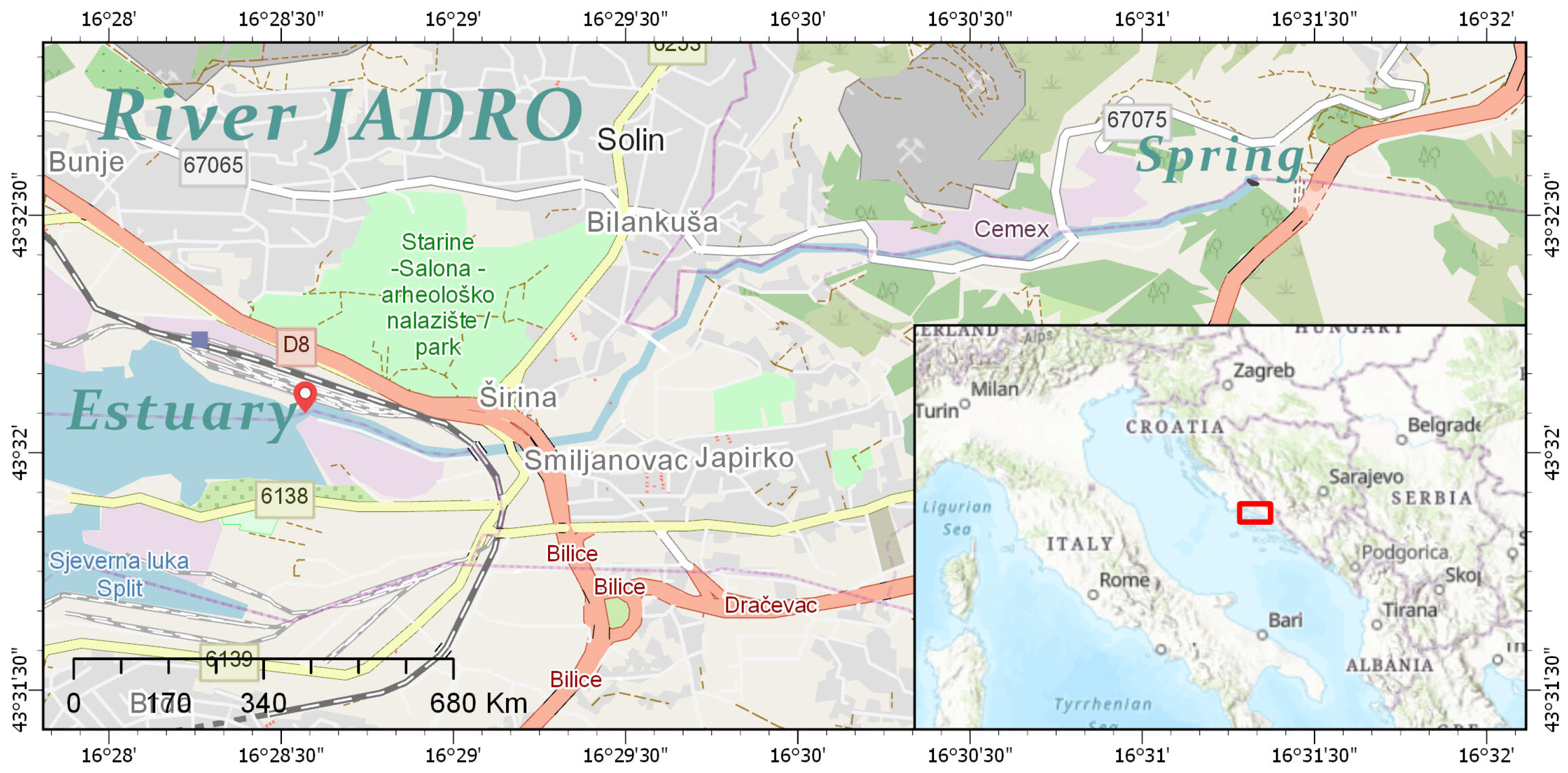
Abstract
:1. Introduction
2. Materials and Methods
2.1. Study Area
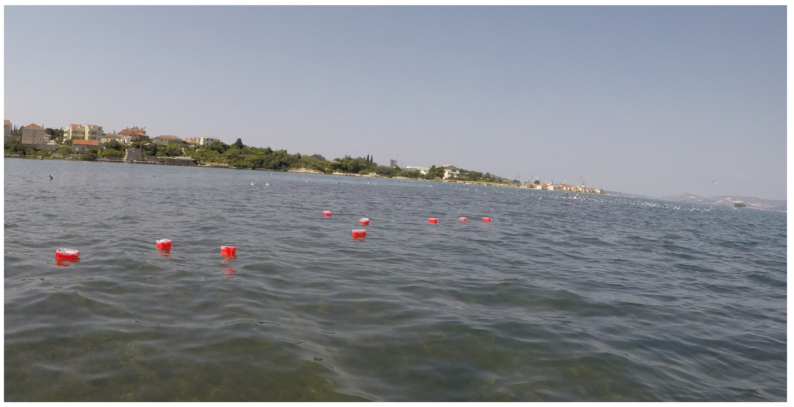
2.2. Field Measurements
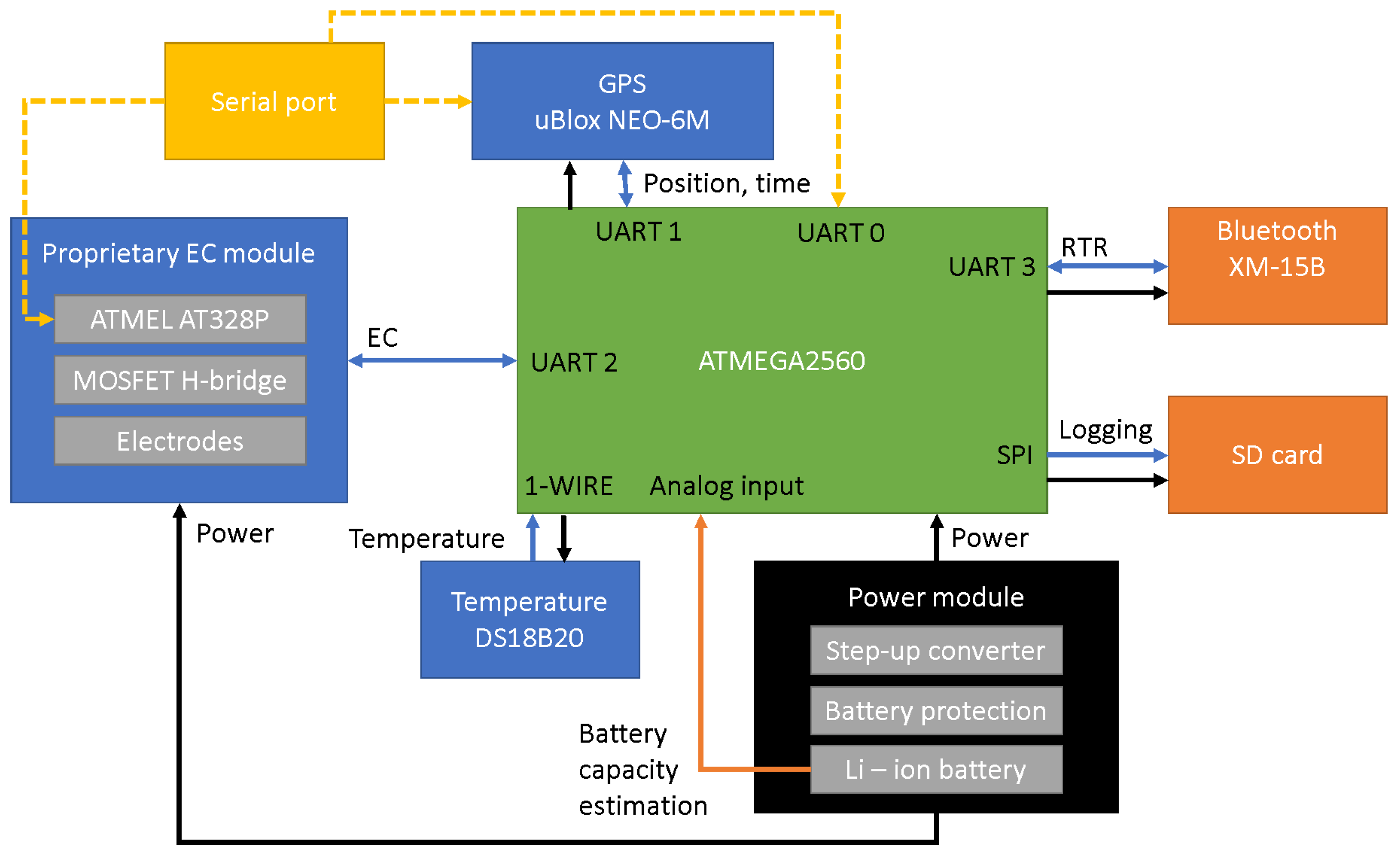
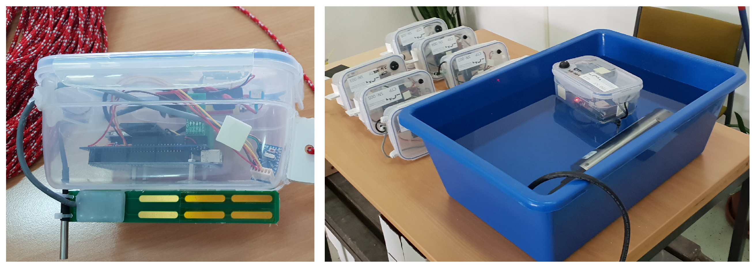
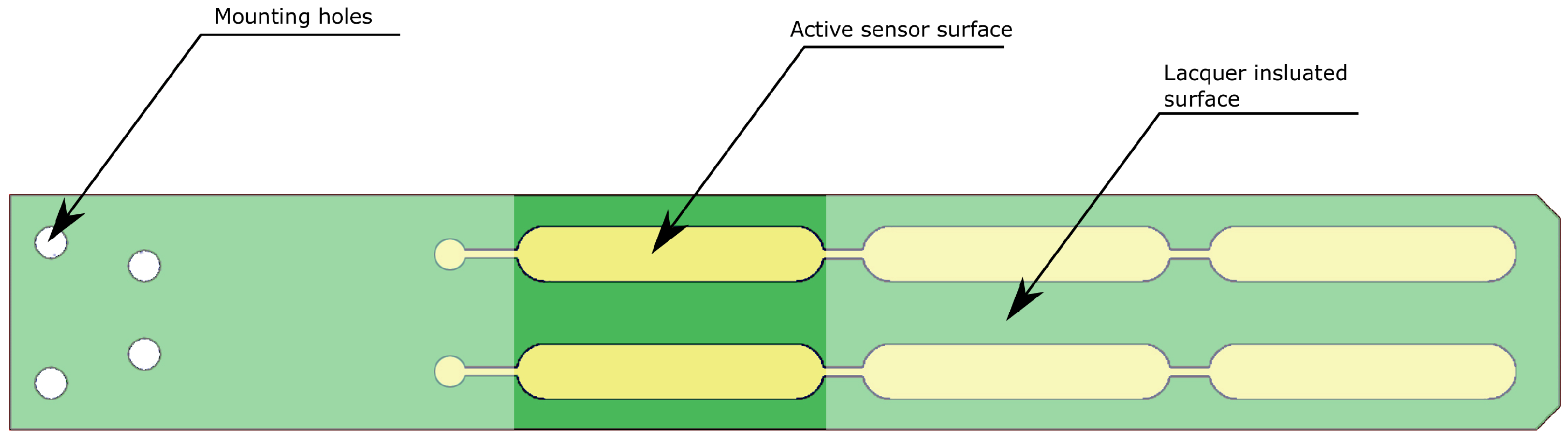
2.3. The Arduino Based Measurement Probe
2.4. Data Processing
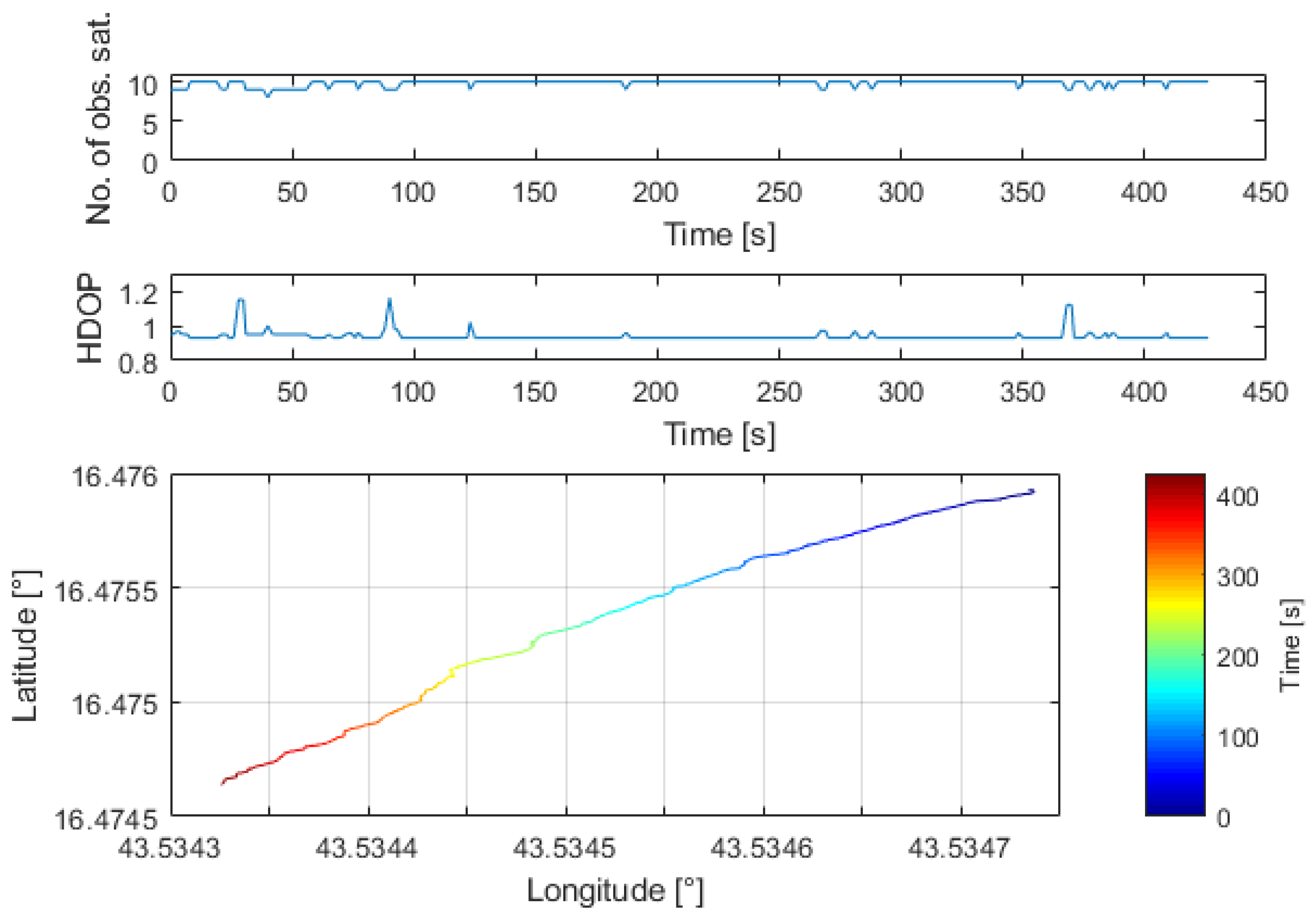
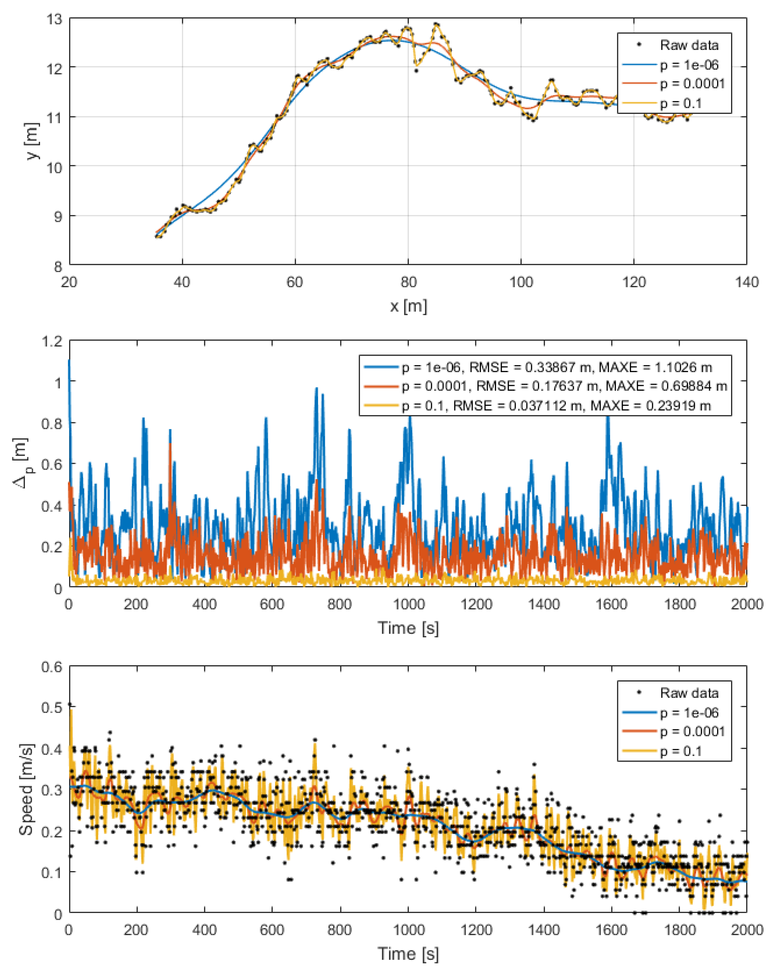
2.4.1. GPS Data
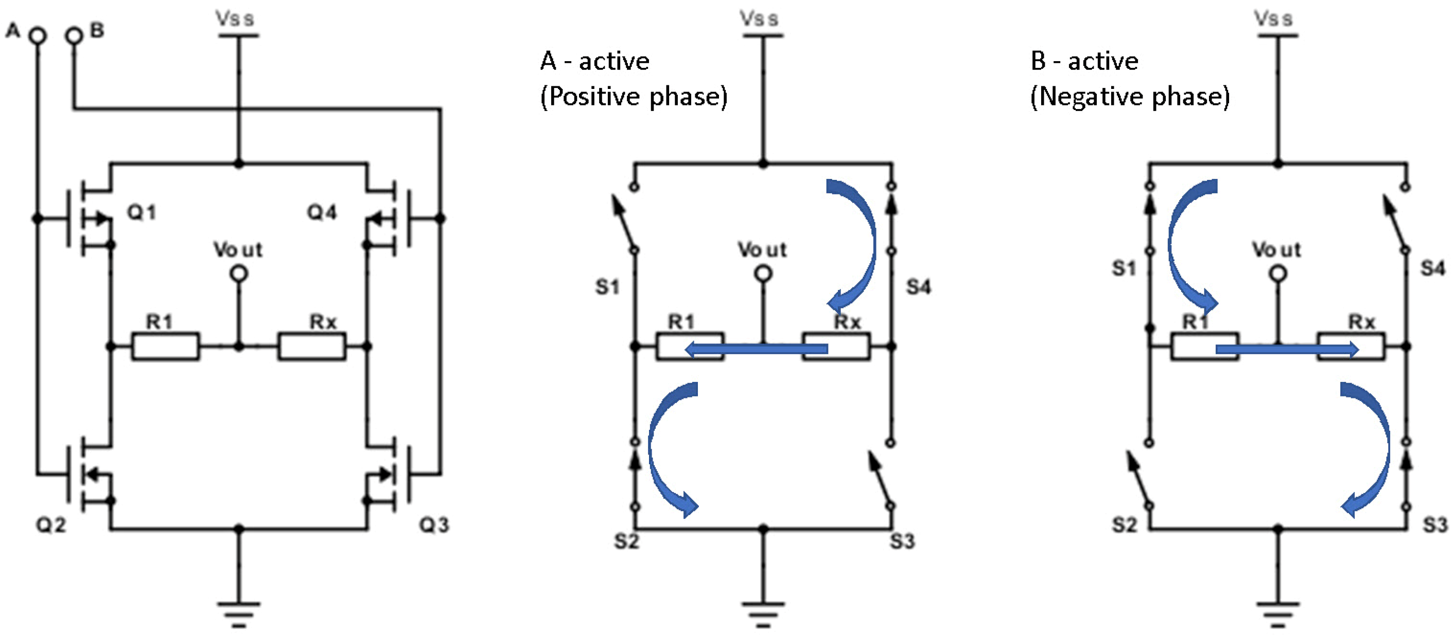
2.4.2. Electrical Conductivity Data
2.4.3. Salinity Data
3. Results
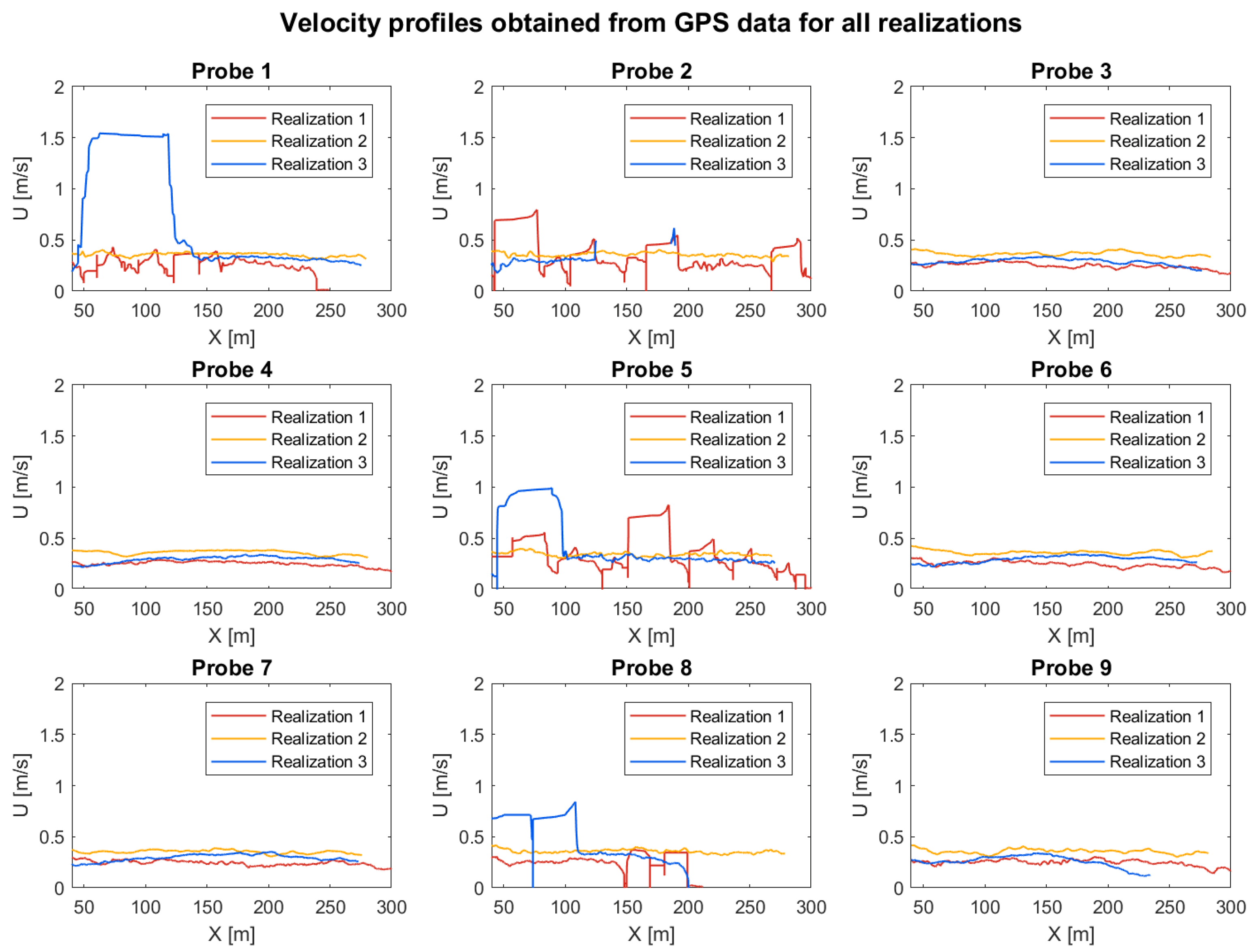
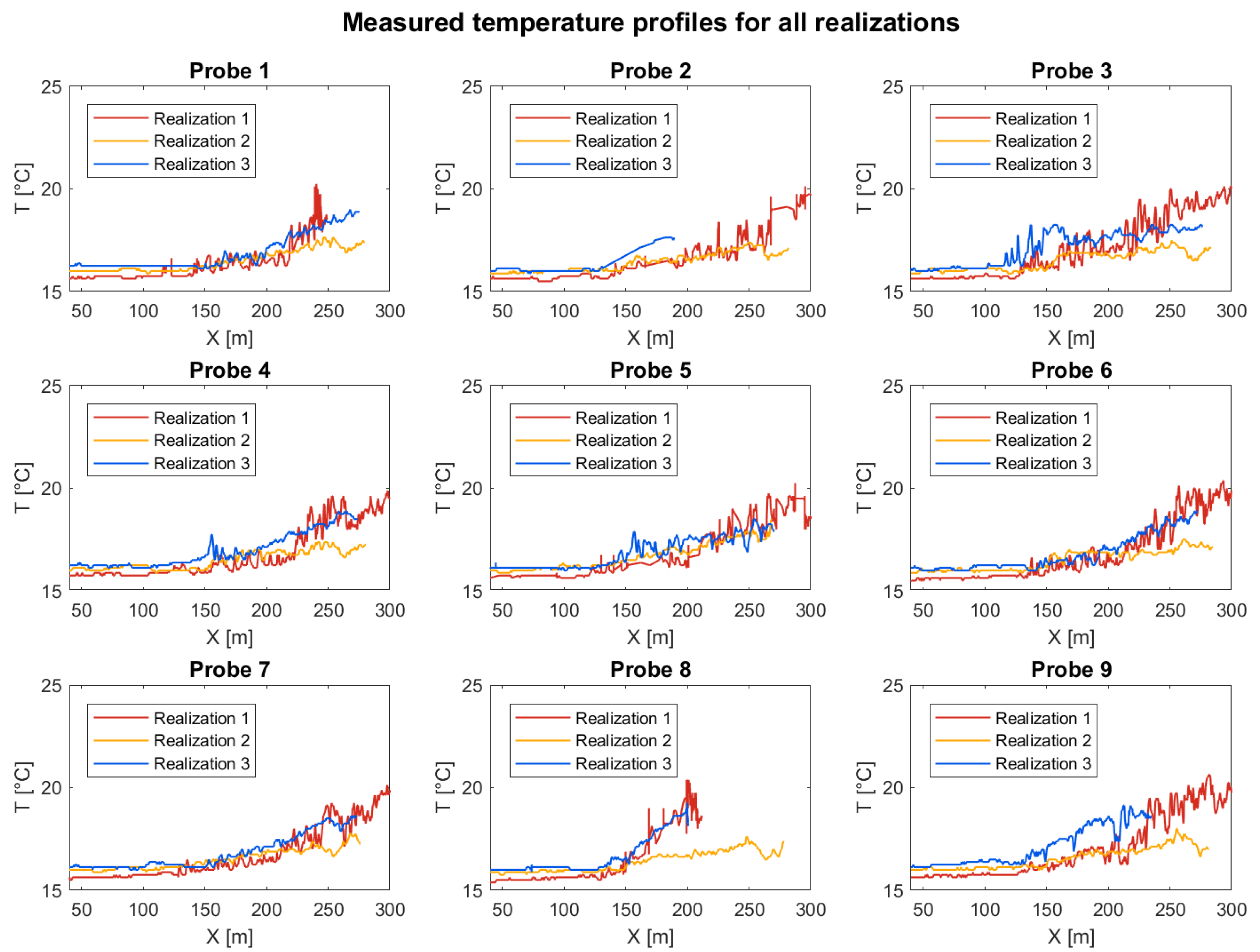
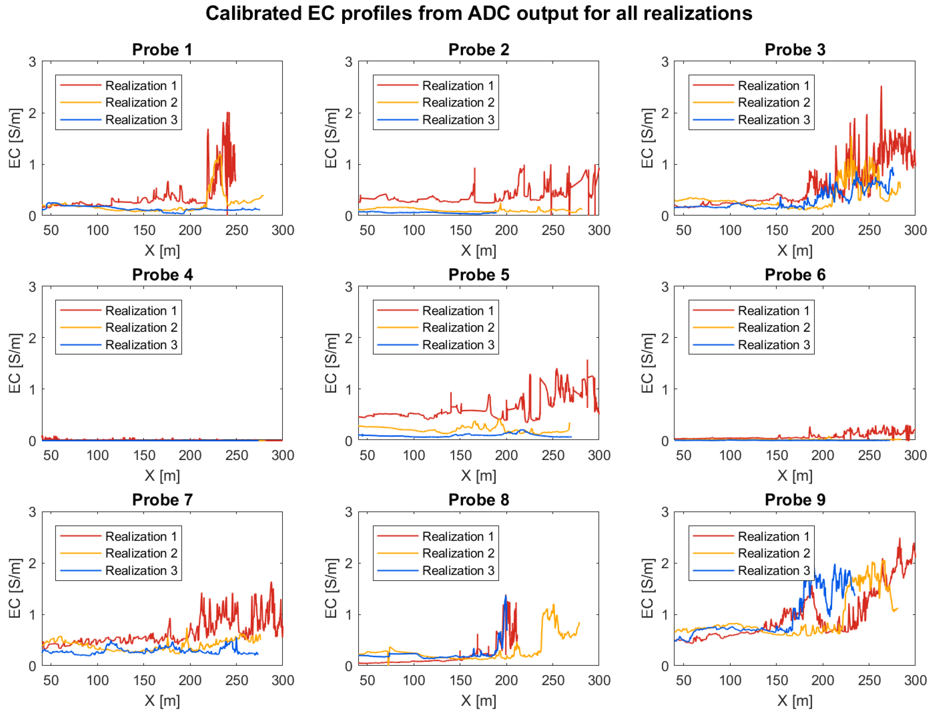
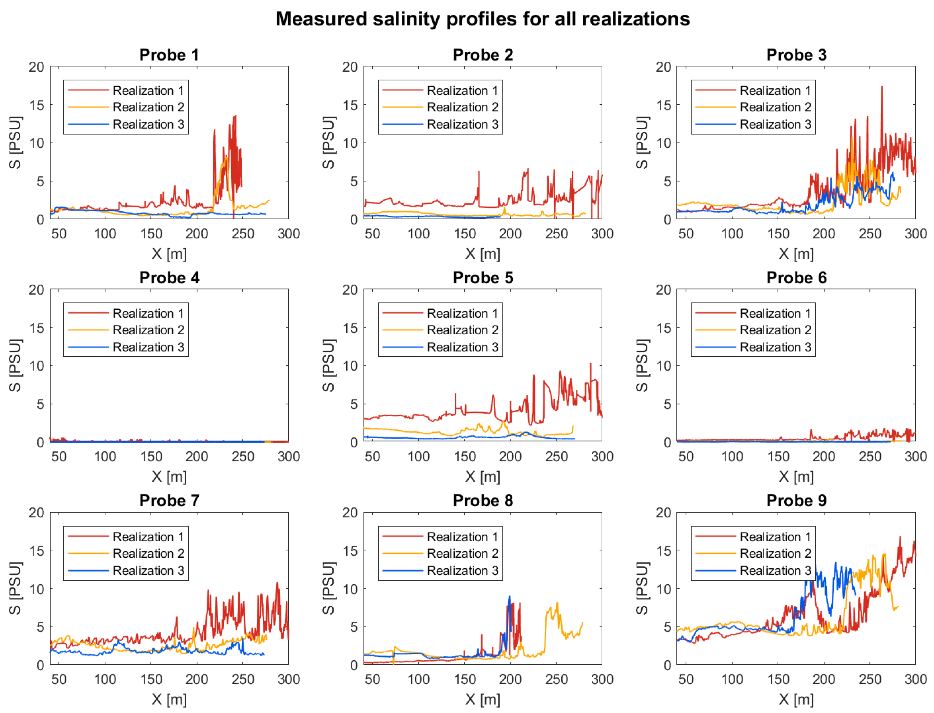
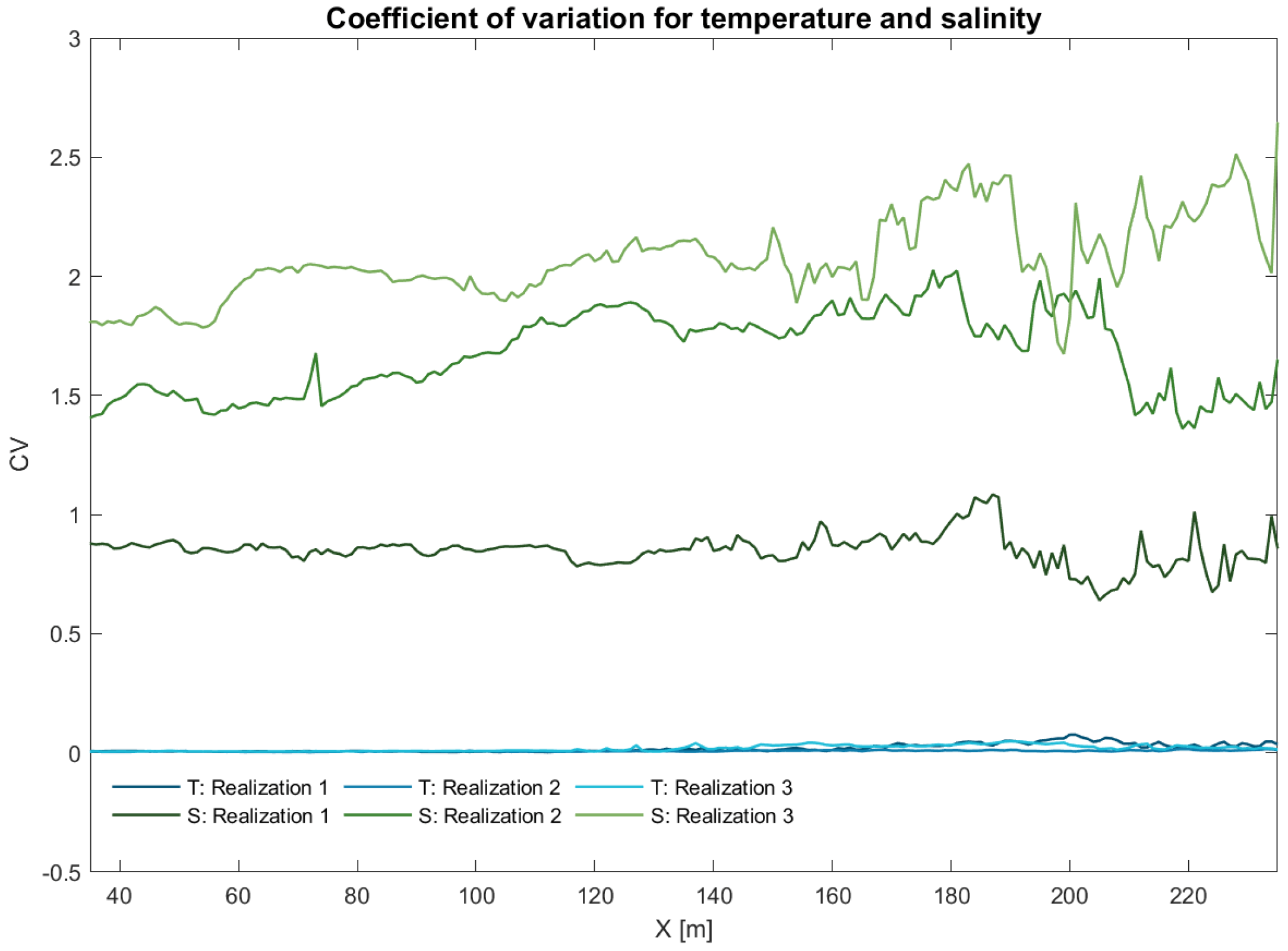
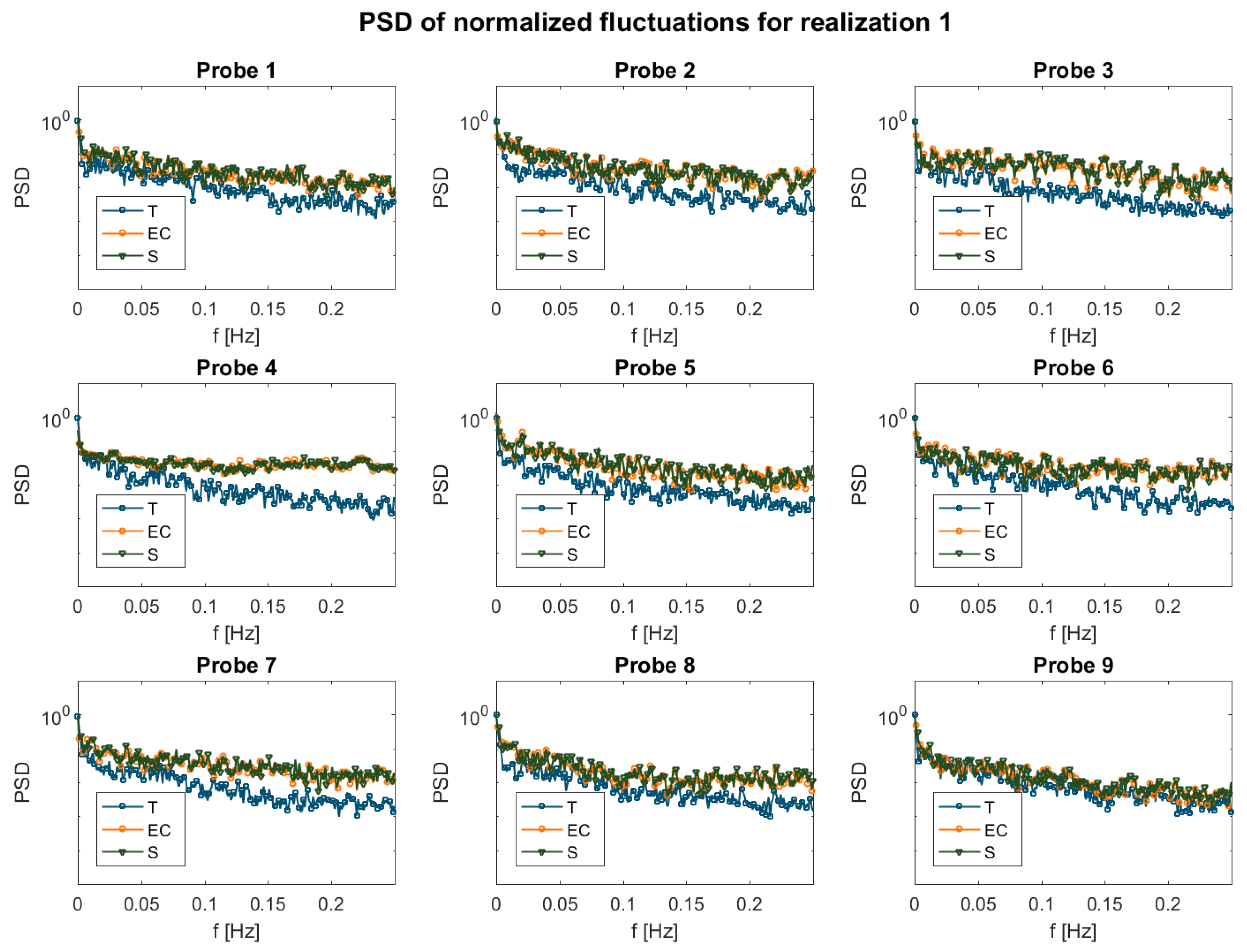
3.1. Measured Data
3.2. Application Potential
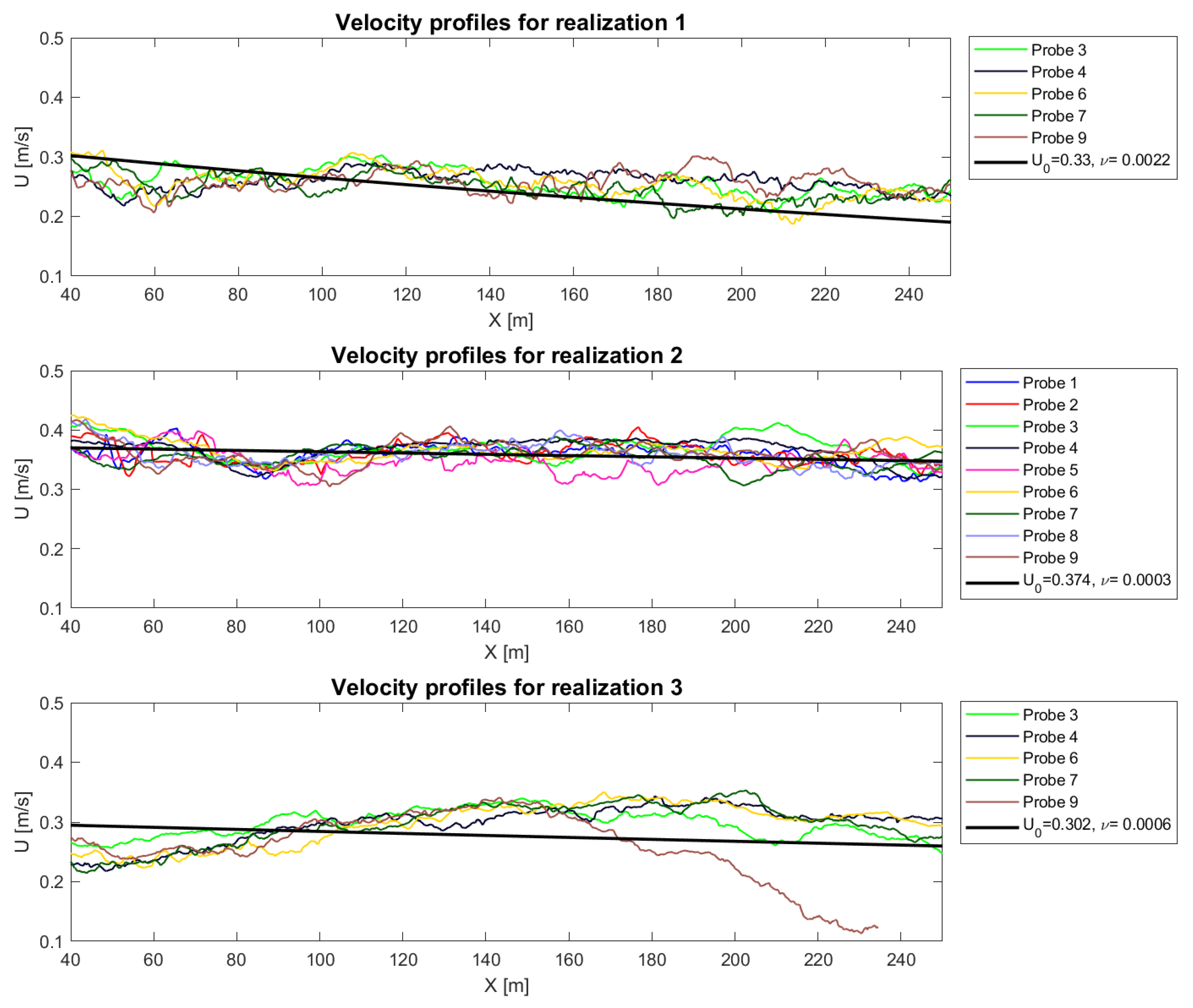
3.2.1. Velocity Model
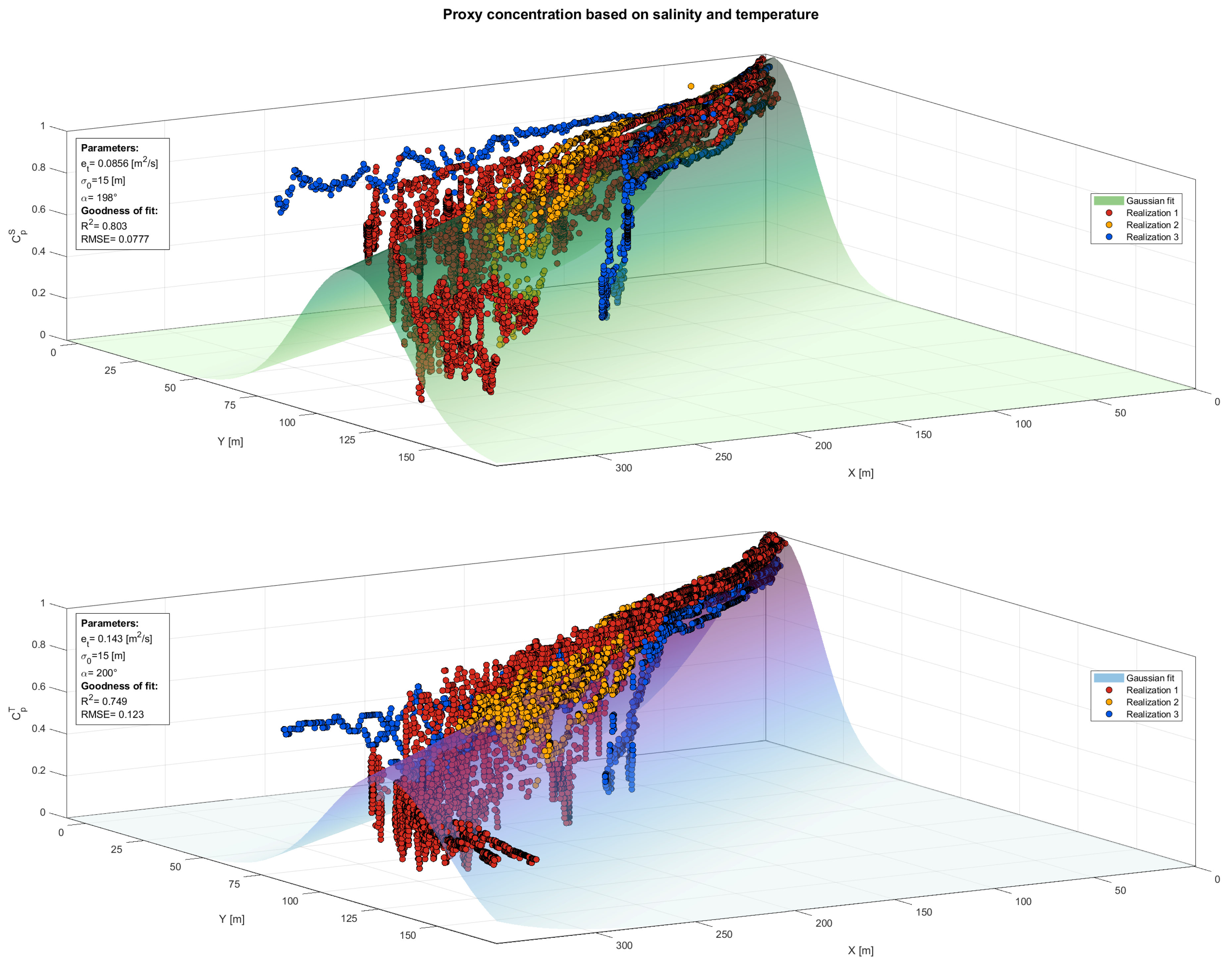
3.2.2. Concentration Proxy
3.3. Discussion and Lessons Learned
4. Conclusions and Future Remarks
Author Contributions
Funding
Acknowledgments
Conflicts of Interest
References
- Elliott, M.; Whitfield, A.K. Challenging paradigms in estuarine ecology and management. Estuar. Coast. Shelf Sci. 2011, 94, 306–314. [Google Scholar] [CrossRef]
- Halpern, B.S.; Walbridge, S.; Selkoe, K.A.; Kappel, C.V.; Micheli, F.; D’agrosa, C.; Bruno, J.F.; Casey, K.S.; Ebert, C.; Fox, H.E.; et al. A global map of human impact on marine ecosystems. Science 2008, 319, 948–952. [Google Scholar] [CrossRef] [PubMed] [Green Version]
- Wolanski, E.; Elliott, M. Estuarine Ecohydrology: An Introduction; Elsevier: Amsterdam, The Netherlands, 2015. [Google Scholar]
- Assessment, M.E. Ecosystems and Human Well-Being; Island Press: Washington, DC, USA, 2005; Volume 5. [Google Scholar]
- Barbier, E.B.; Hacker, S.D.; Kennedy, C.; Koch, E.W.; Stier, A.C.; Silliman, B.R. The value of estuarine and coastal ecosystem services. Ecol. Monogr. 2011, 81, 169–193. [Google Scholar] [CrossRef]
- Barbier, E.B. Progress and Challenges in Valuing Coastal and Marine Ecosystem Services. Rev. Environ. Econ. Policy 2011, 6, 1–19. [Google Scholar] [CrossRef] [Green Version]
- Milon, J.W.; Alvarez, S. The Elusive Quest for Valuation of Coastal and Marine Ecosystem Services. Water 2019, 11, 1518. [Google Scholar] [CrossRef] [Green Version]
- Copeland, C. Clean Water Act: A Summary of the Law; Congressional Research Service, Library of Congress: Washington, DC, USA, 1999.
- European Community. Directive 2000/60/EC of the European Parliament and of the Council of 23 October 2000 Establishing a Framework for Community Action in the Field of Water Policy; Official Journal of the European Communities (L 327/1-73); European Community: Brussels, Belgium, 2000. [Google Scholar]
- European Community. Bathing Water Quality Directive 2006/7/EC; Official Journal of the European Union (OJ L 64); European Community: Brussels, Belgium, 2006. [Google Scholar]
- European Community. Directive 2008/56/EC of the European Parliament and of the Council of 17 June 2008 Establishing a Framework for Community Action in the Field of Marine Environmental Policy (Marine Strategy Framework Directive); Official Journal of the European Union (L 164/19-40); European Community: Brussels, Belgium, 2008. [Google Scholar]
- Guerry, A.D.; Plummer, M.L.; Ruckelshaus, M.H.; Harvey, C.J. Ecosystem service assessments for marine conservation. In Natural Capital: Theory and Practice of Mapping Ecosystem Services; Oxford University Press: Oxford, UK, 2011; pp. 296–322. [Google Scholar]
- Pinto, R.; de Jonge, V.N.; Neto, J.M.; Domingos, T.; Marques, J.C.; Patrício, J. Towards a DPSIR driven integration of ecological value, water uses and ecosystem services for estuarine systems. Ocean. Coast. Manag. 2013, 72, 64–79. [Google Scholar] [CrossRef]
- Tosic, M.; Restrepo, J.D.; Izquierdo, A.; Lonin, S.; Martins, F.; Escobar, R. An integrated approach for the assessment of land-based pollution loads in the coastal zone. Estuar. Coast. Shelf Sci. 2018, 211, 217–226. [Google Scholar] [CrossRef]
- Townsend, M.; Davies, K.; Hanley, N.; Hewitt, J.E.; Lundquist, C.J.; Lohrer, A.M. The Challenge of Implementing the Marine Ecosystem Service Concept. Front. Mar. Sci. 2018, 5, 1–13. [Google Scholar] [CrossRef] [Green Version]
- European, C. Directive 2007/2/EC of the European Parliament and of the Council of 14 March 2007 Establishing an Infrastructure for Spatial Information in the European Community (INSPIRE); Official Journal of the European Communities (L 108/1-14); European Community: Brussels, Belgium, 2007. [Google Scholar]
- Longhorn, R.A. Coastal spatial data infrastructure. In GIS for Coastal Zone Management; CRC Press: Boca Raton, FL, USA, 2004; pp. 1–14. [Google Scholar]
- Tavra, M.; Jajac, N.; Cetl, V. Marine Spatial Data Infrastructure Development Framework: Croatia Case Study. ISPRS Int. J. Geo-Inf. 2017, 6, 117. [Google Scholar] [CrossRef] [Green Version]
- European, C. INSPIRE Geoportal. 2019. Available online: https://inspire-geoportal.ec.europa.eu (accessed on 5 October 2019).
- Borja, A.; Bricker, S.B.; Dauer, D.M.; Demetriades, N.T.; Ferreira, J.G.; Forbes, A.T.; Hutchings, P.; Jia, X.; Kenchington, R.; Marques, J.C.; et al. Overview of integrative tools and methods in assessing ecological integrity in estuarine and coastal systems worldwide. Mar. Pollut. Bull. 2008, 56, 1519–1537. [Google Scholar] [CrossRef]
- Riddle, A.; Lewis, R. Dispersion experiments in UK coastal waters. Estuar. Coast. Shelf Sci. 2000, 51, 243–254. [Google Scholar] [CrossRef]
- Rodriguez, A.; Sánchez-Arcilla, A.; Redondo, J.M.; Bahia, E.; Sierra, J.P. Pollutant dispersion in the nearshore region: Modelling and measurements. Water Sci. Technol. 1995, 32, 169–178. [Google Scholar] [CrossRef]
- Clarke, L.; Ackerman, D.; Largier, J. Dye dispersion in the surf zone: Measurements and simple models. Cont. Shelf Res. 2007, 27, 650–669. [Google Scholar] [CrossRef]
- Galešić, M.; Andričević, R.; Gotovac, H.; Srzić, V. Concentration statistics of solute transport for the near field zone of an estuary. Adv. Water Resour. 2016, 94, 424–440. [Google Scholar] [CrossRef]
- Galešić, M.; Andričević, R.; Divić, V.; Šakić Trogrlić, R. New screening tool for obtaining concentration statistics of pollution generated by rivers in estuaries. Water 2018, 10, 639. [Google Scholar] [CrossRef] [Green Version]
- Plew, D.R.; Zeldis, J.R.; Shankar, U.; Elliott, A.H. Using Simple Dilution Models to Predict New Zealand Estuarine Water Quality. Estuaries Coasts 2018, 41, 1643–1659. [Google Scholar] [CrossRef]
- Estevez, E.D. Review and assessment of biotic variables and analytical methods used in estuarine inflow studies. Estuaries 2002, 25, 1291–1303. [Google Scholar] [CrossRef]
- Savenije, H.H. Salinity and Tides in Alluvial Estuaries; Elsevier: Amsterdam, The Netherlands, 2005; p. 194. [Google Scholar]
- Wiseman, W.J.; Swenson, E.M.; Power, J. Salinity trends in Louisiana estuaries. Estuaries 1990, 13, 265–271. [Google Scholar] [CrossRef]
- Bradley, P.M.; Kjerfve, B.; Morris, J.T.; Kjerfve, B. Rediversion Salinity Change in the Cooper River, South Carolina: Ecological Implications. Estuaries 1990, 13, 373. [Google Scholar] [CrossRef]
- Lorenz, J.J. A review of the effects of altered hydrology and salinity on vertebrate fauna and their habitats in northeastern Florida Bay. Wetlands 2014, 34, 189–200. [Google Scholar] [CrossRef]
- Spalding, E.A.; Hester, M.W. Interactive effects of hydrology and salinity on oligohaline plant species productivity: Implications of relative sea-level rise. Estuaries Coasts 2007, 30, 214–225. [Google Scholar] [CrossRef]
- Rivera-Monroy, V.H.; Twilley, R.R.; Mancera-Pineda, J.E.; Madden, C.J.; Alcantara-Eguren, A.; Moser, E.B.; Jonsson, B.F.; Castañeda-Moya, E.; Casas-Monroy, O.; Reyes-Forero, P.; et al. Salinity and Chlorophyll a as Performance Measures to Rehabilitate a Mangrove-Dominated Deltaic Coastal Region: The Ciénaga Grande de Santa Marta-Pajarales Lagoon Complex, Colombia. Estuaries Coasts 2011, 34, 1–19. [Google Scholar] [CrossRef]
- Little, S.; Wood, P.J.; Elliott, M. Quantifying salinity-induced changes on estuarine benthic fauna: The potential implications of climate change. Estuar. Coast. Shelf Sci. 2017, 198, 610–625. [Google Scholar] [CrossRef] [Green Version]
- Vallino, J.; Hopkinson, J.C.S. Estimation of Dispersion and Characteristic Mixing Times in Plum Island Sound Estuary. Estuar. Coast. Shelf Sci. 1998, 46, 333–350. [Google Scholar] [CrossRef] [Green Version]
- Ho, D.T.; Schlosser, P.; Caplow, T. Determination of Longitudinal Dispersion Coefficient and Net Advection in the Tidal Hudson River with a Large-Scale, High Resolution SF6 Tracer Release Experiment. Environ. Sci. Technol. 2002, 36, 3234–3241. [Google Scholar] [CrossRef]
- Gay, P.; O’Donnell, J. Comparison of the salinity structure of the Chesapeake Bay, the Delaware Bay and Long Island Sound using a linearly tapered advection-dispersion model. Estuaries Coasts 2009, 32, 68–87. [Google Scholar] [CrossRef]
- Xu, J.; Long, W.; Wiggert, J.D.; Lanerolle, L.W.J.; Brown, C.W.; Murtugudde, R.; Hood, R.R. Climate Forcing and Salinity Variability in Chesapeake Bay, USA. Estuaries Coasts 2012, 35, 237–261. [Google Scholar] [CrossRef]
- Troselj, J.; Sayama, T.; Varlamov, S.M.; Sasaki, T.; Racault, M.F.; Takara, K.; Miyazawa, Y.; Kuroki, R.; Yamagata, T.; Yamashiki, Y. Modeling of extreme freshwater outflow from the north-eastern Japanese river basins to western Pacific Ocean. J. Hydrol. 2017, 555, 956–970. [Google Scholar] [CrossRef]
- Andričević, R.; Galešić, M. Contaminant dilution measure for the solute transport in an estuary. Adv. Water Resour. 2018, 117, 65–74. [Google Scholar] [CrossRef]
- Galešić, M.; Andričević, R.; Divić, V.; Mateus, M.; Pinto, L. Potential data used for validation of concentration statistics obtained using analytical model for conservative transport in an estuary. EGU General Assembly 2016. Water Resour. 2016, 31, 714–725. [Google Scholar]
- Galešić, M. Concentration Statistics for Conservative Solute Transport in River Estuaries. Ph.D. Thesis, University of Split, Split, Croatia, 2018. [Google Scholar]
- Albaladejo, C.; Soto, F.; Torres, R.; Sánchez, P.; López, J.A. A low-cost sensor buoy system for monitoring shallow marine environments. Sensors 2012, 12, 9613–9634. [Google Scholar] [CrossRef]
- Marcelli, M.; Piermattei, V.; Madonia, A.; Mainardi, U. Design and application of new low-cost instruments for marine environmental research. Sensors 2014, 14, 23348–23364. [Google Scholar] [CrossRef] [Green Version]
- Arduino. What is Arduino. 2019. Available online: https://www.arduino.cc/en/Guide/Introduction (accessed on 5 October 2019).
- Lockridge, G.; Dzwonkowski, B.; Nelson, R.; Powers, S. Development of a low-cost arduino-based sonde for coastal applications. Sensors 2016, 16, 528. [Google Scholar] [CrossRef] [Green Version]
- Legović, T. Exchange of water in a stratified estuary with an application to Krka (Adriatic Sea). Mar. Chem. 1991, 32, 121–135. [Google Scholar] [CrossRef]
- Ljubenkov, I.; Vranješ, M. Zaslanjivanje ušća rijeke Jadro - mjerenje i hidrodinamičko modeliranje. Hrvat. Vode 2013, 545, 225–234. [Google Scholar]
- Krvavica, N.; Travaš, V.; Ravlić, N.; Ožanić, N. Hydraulics of Stratified Two-layer Flow in Rječina Estuary. In Proceedings of the Landslides and Flood Hazard Assessment, Zagreb, Croatia, 6–9 March 2013; pp. 1–5. [Google Scholar]
- Montagna, P.; Palmer, T.A.; Pollack, J.B. Hydrological Changes and Estuarine Dynamics; Springer Science & Business Media: Berlin, Germany, 2012; Volume 8. [Google Scholar]
- IZOR. Institute of Oceanography and Fisheries. 2019. Available online: http://www.izor.hr/ (accessed on 2 December 2019).
- KeuwlsoftElectronics. 2019. Available online: http://www.keuwl.com/electronics.html (accessed on 5 October 2019).
- ConductivityKit. 2019. Available online: https://www.atlas-scientific.com (accessed on 2 December 2019).
- Microchip. 2019. Available online: https://www.microchip.com/wwwproducts/en/ATmega2560 (accessed on 5 October 2019).
- National Marine Electronics Association. 2019. Available online: https://www.nmea.org (accessed on 5 October 2019).
- MaximIntegrated. 2019. Available online: https://www.maximintegrated.com/en/products/sensors/DS18B20.html (accessed on 5 October 2019).
- U-blox. NEO-6 Series. 2019. Available online: https://www.u-blox.com/en/product/neo-6-series (accessed on 5 October 2019).
- Jun, J.; Guensler, R.; Ogle, J.H. Smoothing methods to minimize impact of global positioning system random error on travel distance, speed, and acceleration profile estimates. Transp. Res. Rec. 2006, 1972, 141–150. [Google Scholar] [CrossRef]
- De Boor, C. A Practical Guide to Splines; Springer: New York, NY, USA, 1978; Volume 27. [Google Scholar]
- Antonov, J. World Ocean Atlas 2005, Volume 2: Salinity; NOAA Atlas NESDros. Information Service: Silver Spring, MD, USA, 2006; Volume 62. [Google Scholar]
- Perkin, R.; Lewis, E. The Practical Salinity Scale 1978: Fitting the data. IEEE J. Ocean. Eng. 1980, 5, 9–16. [Google Scholar] [CrossRef]
- Jones, G.R.; Nash, J.D.; Doneker, R.L.; Jirka, G.H. Buoyant surface discharges into water bodies. I: Flow classification and prediction methodology. J. Hydraul. Eng. 2007, 133, 1010–1020. [Google Scholar] [CrossRef]
- MacCready, P.; Geyer, W.R. Advances in Estuarine Physics. Annu. Rev. Mar. Sci. 2009, 2, 35–58. [Google Scholar] [CrossRef] [PubMed] [Green Version]
- Kuo, A.Y.; Neilson, B.J. Hypoxia and Salinity in Virginia Estuaries. Estuaries 1987, 10, 277. [Google Scholar] [CrossRef]
- Trancart, T.; Feunteun, E.; Lefrançois, C.; Acou, A.; Boinet, C.; Carpentier, A. Difference in responses of two coastal species to fluctuating salinities and temperatures: Potential modification of specific distribution areas in the context of global change. Estuar. Coast. Shelf Sci. 2016, 173, 9–15. [Google Scholar] [CrossRef] [Green Version]
- Pulina, S.; Satta, C.T.; Padedda, B.M.; Sechi, N.; Lugliè, A. Seasonal variations of phytoplankton size structure in relation to environmental variables in three Mediterranean shallow coastal lagoons. Estuar. Coast. Shelf Sci. 2018, 212, 95–104. [Google Scholar] [CrossRef]
- Ozsoy, E.; Unluata, U. Ebb-tidal flow characteristics near inlets. Estuar. Coast. Shelf Sci. 1982, 14, 251-IN3. [Google Scholar] [CrossRef]
- MARETEC-IST. 2019. Available online: http://www.mohid.com (accessed on 5 October 2019).
- O’Shea, M.L.; Brosnan, T.M. Trends in Indicators of Eutrophication in Western Long Island Sound and the Hudson-Raritan Estuary. Estuaries 2000, 23, 877. [Google Scholar] [CrossRef]
- Araujo, A.V.; Dias, C.O.; Bonecker, S.L. Effects of environmental and water quality parameters on the functioning of copepod assemblages in tropical estuaries. Estuar. Coast. Shelf Sci. 2017, 194, 150–161. [Google Scholar] [CrossRef]
- Fischer, H.B.; List, J.E.; Koh, C.R.; Imberger, J.; Brooks, N.H. Mixing in Inland and Coastal Waters; Academic Press: Cambridge, MA, USA, 1979; p. 302. [Google Scholar]
- Sawford, B.; Sullivan, P. A simple representation of a developing contaminant concentration field. J. Fluid Mech. 1995, 289, 141–157. [Google Scholar] [CrossRef]
- Sullivan, P.J. The influence of molecular diffusion on the distributed moments of a scalar PDF. Environmetrics 2004, 15, 173–191. [Google Scholar] [CrossRef]
- Di Dato, M.; Galešić, M.; Šimundić, P.; Andričević, R. A novel screening tool for the health risk in recreational waters near estuary: The Carrying Capacity indicator. Sci. Total. Environ. 2019, 694, 133584. [Google Scholar] [CrossRef]
- Rutherford, J. River Mixing; John Wiley & Sons Ltd.: Chichester, UK, 1994. [Google Scholar]
- Ippen, A.; Eagleson, P. Estuary and Coastline Hydrodynamics; Engineering Societies Monographs; McGraw-Hill Book Co.: New York, NY, USA, 1966. [Google Scholar]
- Savenije, H.H. Prediction in ungauged estuaries: An integrated theory. Water Resour. Res. 2015, 51, 2464–2476. [Google Scholar] [CrossRef] [Green Version]
- Jacobsen, E.; Lyons, R. An update to the sliding DFT. IEEE Signal Process. Mag. 2004, 21, 110–111. [Google Scholar] [CrossRef]
- Lyons, R.G. Understanding Digital Signal Processing, 3/E; Pearson Education India: London, UK, 2004. [Google Scholar]


© 2020 by the authors. Licensee MDPI, Basel, Switzerland. This article is an open access article distributed under the terms and conditions of the Creative Commons Attribution (CC BY) license (http://creativecommons.org/licenses/by/4.0/).
Share and Cite
Divić, V.; Galešić, M.; Di Dato, M.; Tavra, M.; Andričević, R. Application of Open Source Electronics for Measurements of Surface Water Properties in an Estuary: A Case Study of River Jadro, Croatia. Water 2020, 12, 209. https://doi.org/10.3390/w12010209
Divić V, Galešić M, Di Dato M, Tavra M, Andričević R. Application of Open Source Electronics for Measurements of Surface Water Properties in an Estuary: A Case Study of River Jadro, Croatia. Water. 2020; 12(1):209. https://doi.org/10.3390/w12010209
Chicago/Turabian StyleDivić, Vladimir, Morena Galešić, Mariaines Di Dato, Marina Tavra, and Roko Andričević. 2020. "Application of Open Source Electronics for Measurements of Surface Water Properties in an Estuary: A Case Study of River Jadro, Croatia" Water 12, no. 1: 209. https://doi.org/10.3390/w12010209