Multi-Indicator Evaluation for Extreme Precipitation Events in the Past 60 Years over the Loess Plateau

1
Institute for Energy, Environment and Sustainability Research, UR-NCEPU, North China Electric Power University, Beijing 102206, China
2
Center for Energy, Environment and Ecology Research, UR-BNU, Beijing Normal University, Beijing 100875, China
3
College of Engineering, Design and Physical Sciences, Brunel University, London, Uxbridge, Middlesex UB8 3PH, UK
*
Author to whom correspondence should be addressed.
Water 2020, 12(1), 193; https://doi.org/10.3390/w12010193
Submission received: 15 November 2019
/
Revised: 15 December 2019
/
Accepted: 6 January 2020
/
Published: 10 January 2020
(This article belongs to the Special Issue Modeling and Monitoring Climate Extremes and Impacts on Natural-Human Systems)
Abstract
:The unique characteristics of topography, landforms, and climate in the Loess Plateau make it especially important to investigate its extreme precipitation characteristics. Daily precipitation data of Loess Plateau covering a period of 1959–2017 are applied to evaluate the probability features of five precipitation indicators: the amount of extreme heavy precipitation (P95), the days with extreme heavy precipitation, the intensity of extreme heavy precipitation (I95), the continuous dry days, and the annual total precipitation. In addition, the joint risk of different combinations of precipitation indices is quantitatively evaluated based on the copula method. Moreover, the risk and severity of each extreme heavy precipitation factor corresponding to 50-year joint return period are achieved through inverse derivation process. Results show that the precipitation amount and intensity of the Loess Plateau vary greatly in spatial distribution. The annual precipitation in the northwest region may be too concentrated in several rainstorms, which makes the region in a serious drought state for most of the year. At the level of 10-year return period, more than five months with no precipitation events would occur in the Northwest Loess Plateau. While, P95 or I95 events of 100-year level may be encountered in a 50-year return period and in the southeastern region, which means there are foreseeable long-term extreme heavy precipitation events.
1. Introduction
In the past half century, extreme precipitation events have increased remarkably and may be more frequent and severe over the mid-latitudes in the context of global warming [1,2,3]. Extreme precipitation events contain extreme strong precipitation and extreme weak precipitation. Large amounts of precipitation due to heavy precipitation can converge rapidly in steep slope areas, which often bring floods, mudslides, and other secondary disasters [4,5]. Extreme weak precipitation is the occurrence of no precipitation or very little precipitation for a long time, which can cause long-term droughts to the region. Both extreme heavy rainfall and drought events can cause severe agricultural, environmental, and socioeconomic losses and may pose a serious threat to human life. Therefore, it is very valuable to address the extreme precipitation, identify the areas where floods and droughts may occur, and reveal their occurrence rules. All these efforts can provide priceless support for reasonable disaster mitigation measures and water resources management [6,7].
Recently, properties of extreme precipitation have been extensively explored in many places of the world. The commonly used techniques to identify the extreme precipitation events are the absolute threshold method and the percentile method, in which the extreme precipitation events are identified by a fixed value and a certain percentile value of precipitation sequence, respectively [8,9,10]. In general, many research studies analyzed the spatial and temporal differences in terms of number of days with extreme precipitation, the amount of extreme precipitation and extreme precipitation intensity [8,11,12]. These studies can reveal the features of single precipitation factors and also indicate that extreme precipitation events are affected by many indicators [12]. However, traditional approaches are generally subjective and cannot quantitatively assess the risk of extreme precipitation. In addition, the correlated features of different extreme precipitation indicators are often ignored. Therefore, it is necessary to explore the relationship between the representative combinations of extreme precipitation factors, identify their characteristics, and quantitatively evaluate their individual and joint risks.
The joint behavior of different risk indicators has been paid widespread attention and studied in various fields, especially in hydrology [13,14,15,16]. As a powerful multidimensional statistical analysis method, copulas have a wide range of applications in various fields and are commonly used to assess the joint probabilistic behaviors of hydrological or meteorological features in hydrometeorological studies [17,18,19]. The copula function permits modeling the individual behaviors and dependence structures separately and the marginal distributions of individual indicators do not need to be unified [12]. The joint probability distributions of different risk indicators and the joint return periods of extreme events at different severities are often presented as quantitative risk assessment results [20,21]. However, by giving fixed extreme indicator values of certain recurrence periods, the obtained joint return periods based on copulas ways tend to be too small or too large [22,23]. Smaller ones do not accurately reflect the severity of the incident, while too large values, such as the joint recurrence period of hundreds of years or even thousands of years, make the results meaningless. In addition, an extremely large joint return period also indicates that this event is too close to the tail of the joint distribution, which makes the calculation results unreliable. Therefore, it is desirable to obtain the severity of the event under a large joint recurrence period within a reasonable range, so that the severity of the extreme event can be accurately assessed while ensuring that the assessment results are credible. This prompted us to propose a climate risk assessment framework, using copula-based methods to reveal the intrinsic characteristics of variables and establish a reverse calculation process to evaluate the severity of indicators given the joint return period of interest.
Being located in the north central part of China, the Loess Plateau is selected as the research area because of its several unique characteristics: first, the topography of the Loess Plateau is complex, which is characterized by steep slopes, high mountains, and a crisscross network of ravines with the extreme heavy precipitation rapidly converging [24,25]. Second, the spatial distribution of precipitation on the Loess Plateau is severely uneven and the climate changes from arid to semi humid along the direction of the northwest–southeast [25]. In addition, the trend of the topography shows a decline from the northwest to the southeast, which makes water resources more unbalanced in this region. The study of the extreme precipitation characteristics over the Loess Plateau is particularly helpful to analyze the risk of drought and flood in this area. Third, being covered by the largest loess layer in the world, the thick and loose loess has made this region the world’s most severe soil erosion area, and soil erosion caused by a strong storm can account for 60%–90% of soil erosion throughout the year [25,26,27]. All these reasons above make it necessary to analyze the features of extreme precipitation in this area.
The purpose of this paper is to quantitatively evaluate the joint risk of multiple extreme precipitation indicators in the Loess Plateau and make a comprehensive description of the multi-type risks. In order to achieve this goal, different marginal distribution functions are employed to fit the distributions of the extreme precipitation indicators and different copulas are applied to establish their joint probability distributions. The risk of single indicators and multiple indicator combinations at different severity levels are quantitatively evaluated. The risk and severity of each extreme heavy precipitation index are obtained through inverse derivation process from a reasonable given joint return period of interest.
2. Study Area and Data
The Loess Plateau is located in the north central part of China (as shown in Figure 1), with a total area of about 6.4 × 10⁵ km2 [25]. In terms of topography, most areas of the hilly-gullied Loess Plateau are between 1000 and 1500 m above sea level [28]. The overall trend of the topography over the Loess Plateau is mainly characterized by a wavy decline from the northwest to the southeast. In terms of landforms, except for a few stony mountainous regions, the Loess Plateau has the most widely distributed loess landform. The thickness of loess is generally between 50 and 80 m, and the maximum thickness part is 150–180 m. The slope terrain with loose structure and low vegetation coverage make the soil erosion intensive and the ecological environment fragile.
Being located on the edge of the warm temperate monsoon climate zone and affected by the semi-arid continental monsoon climate, the Loess Plateau is cold and dry in winter, and warm and rainy in summer. From southeast to northwest, the Loess Plateau would experience warm temperate semi-humid climates, semi-arid climates, and arid climates in turn. The average annual temperature of the Loess Plateau is 8–14 °C, and the annual precipitation is 600–800 mm of which more than 60% is concentrated in July–September [29]. The average relative variability of annual precipitation is between 20% and 30%, the total amount of precipitation in the wet years may be several times or even dozens of times of the total precipitation in the dry years. The quantity of precipitation throughout seasons is uneven, the precipitation in winter would generally accounting for only 3%–5% of the total annual precipitation, and the precipitation in summer and autumn would account for 60%–80% of the total annual precipitation.
The time series of daily precipitation data for 69 weather stations across the Loess Plateau (Figure 1) were obtained from the China Meteorological Administration (http://cdc.cma.gov.cn), covering the period from 1959 to 2017. The spatial distribution of the selected stations is relatively uniform, and the obtained data were checked for homogeneity based on Relative Homogeneity test [30]. Missing data, especially in the rainy season, would affect the calculation of extreme precipitation indexes. The ratio of missing precipitation data in rainy season of July–September over all stations is from 0.07% to 0.5%, with an average of 0.21%. The missing data were replaced by average precipitation of adjacent stations, and thus the calculation of extreme indexes in this study would be affected very little [31]. The days with precipitation <1 mm were considered as no-rain days and the days with precipitation ≥1 mm were considered as rainy days.
3. Method
3.1. Marginal Distribution and Univariate Return Period
To quantify the probabilistic feature for a particular random variable, on account of the selection criteria, the marginal distribution is usually constructed by choosing the best fitted distribution among a set of preassigned distributions such as Pearson type III (P3), lognormal (LN), Log Pearson type III (LP III) [21,32]. In this study, the general extreme value (GEV) distribution, Gamma, P3, LN, LP III, and Weibull distributions were the candidate models which were applied to quantify the probabilistic characteristics for different extreme precipitation indicators. The unknown marginal distribution parameters were estimated through the maximum likelihood estimation (MLE) method. The root mean square error (RMSE), Kolomogorov–Smirnov (KS) test, and Akaike’s information criteria (AIC, [33]) were used for testing and selecting the best fitted marginal distribution among the pre-assigned marginal distributions. The AIC and RMSE can be obtained as follows
where MSE is the mean square error, N is the length of the random variable; k represents the number of the unknown parameters in the distribution models; denotes the theoretical values obtained from the fitted distribution; stands for the non-exceedance probabilities derived from the Gringorten plotting position formula [34] which is expressed as:
where l stands for the lth smallest observation and the observations are arranged in an ascending order.
Once the marginal distributions are fitted for the extreme precipitation indicators, the risk of extreme precipitation indices can be quantitatively assessed based on the univariate return period (RP). The RP of an extreme precipitation index is described as the time between two consecutive events. The formula of single variable return period that used in this study is shown as:
where F(x) is the cumulative distribution functions (CDF) of precipitation indicator and ranges between 0 and 1; / represents the RP of precipitation indicator with value greater/less than or equal to a certain value of x.
3.2. Construction of Joint Distribution of Extreme Precipitation Indicators
In reality, precipitation events tend to show diverse characteristics, which are described by different indicators. Additionally, these indicators of precipitation always have a correlation in different degrees. The separated analysis of multiple indicators often can neither reveal the correlation among them, nor quantify the joint risk of the correlated indicators. In this study, copula functions were considered to build interdependence relationships between different precipitation indicators. The copulas are powerful techniques which can flexibly construct multivariate joint distributions based on the marginal distributions of related variables. Based on the theory of copula function proposed by Sklar [35], the joint probability distribution of two correlated random variables can be expressed as [36]:
where x, y are the values of random variables X and Y, respectively; FX and FY refer to marginal CDFs of the random vector (X, Y). A copula function C exists when the marginal distributions are continuous, and it can be expressed as [37]:
where u = F(x) and v = F(y), (u, v ∈ [0, 1]). Nelsen [35] gives more details on the characteristics of copulas.
Many copula families, including elliptical, Archimedean, and extreme value copulas can be applied in practical multivariate analysis. The well-known Gaussian copula, t copula which belongs to the elliptical family, and four Archimedean copulas (Joe, Gumbel, Clayton, and Frank) were adopted in this study [38]. These copulas were employed due to their capabilities of capturing various kinds of dependence structures. In the case of the precipitation indicators, different precipitation indices show distinct relationships (positively or negatively correlated) and the chosen copulas are able to reflect these complex interrelationships [22]. The parameters of copula functions were estimated through the MLE approach. The KS test, AIC, and RMSE measures were then used for testing and selecting the best fitted copula.
3.3. Bivariate Return Periods of Extreme Precipitation Indicators
The mathematical calculation of RP for single variable is given in Equation (3), which is used to calculate the theoretical recurrence time periods for each precipitation index corresponding to different severity. For multiple correlated variables, once the marginal distributions and joint distributions are obtained, the joint RPs can be estimated based on the different combination types of the variables. Salvadori and de Michele [39] have introduced and discussed the concept of bivariate RPs. In this study, the following three kinds of joint RPs were investigated for different combinations of correlated variables:
where T {X > x, Y > y} represents the bivariate RP when both X and Y exceed the specific values (i.e., X ≥ x and Y ≥ y); T {X > x or Y ≥ y} denotes the RP with X exceeding the threshold of x or Y exceeding the threshold of y. T {X > x, Y ≤ y} represents the joint RP of the event that X is higher than a certain threshold x and Y is smaller than and equal to a certain value y.
It is worthy to notice that previous studies have often calculated the joint risk using specific values of marginal CDFs and thus the calculated joint RPs of all stations in the region are often too small or too large. Excessive return periods often indicate that the critical events under current selected severity are extremely unlikely to happen or the results are not credible because the CDF values are too close to the tail. Although a very small bivariate RP indicates that the event is at a high risk of joint occurrence, it cannot provide the severity of the event corresponding to a larger joint recurrence period within a reasonable range, and thus may underestimate the severity of the joint risk. In this case, the severity of the event should be quantitatively estimated under a selected joint return period. Here the inverse calculation processes corresponding to Equations (6)–(8) are respectively shown as:
As can be seen from the formulas above, in the case when the joint RPs are known, the right side of the formulas can be known, and infinite combinations of u and v can then be obtained. In the case the univariate return periods are set equal to each other, the fixed marginal CDF values can be derived based on golden section search and parabolic interpolation method [40]. The univariate return period and the specific variable values corresponding to the marginal distributions can then be calculated.
4. Method Application and Results Analyses
To quantify the multiple characteristics of extreme precipitation in the study area, a set of suitable indices are desired. Many candidate extreme precipitation indices have been used in the past research works [41,42]. Considering the fact that precipitation in the Loess Plateau is generally low but concentrated in the rainy season, the selected indicator set is expected to contain both indices that could describe the severity of drought and indices that could reflect extreme heavy rainfall. For the objective of this, the potential indices of the amount of extreme heavy precipitation (P95), the days with extreme precipitation (D95), and the intensity of extreme heavy precipitation (I95) were used to reflect extreme heavy rainfall. The continuous dry days (CDD) was selected as the index to reflect the degree of drought. In addition, the annual total precipitation PRTOT was also chosen because it can flexibly reflect the degree of drought and humidity of the climate. These chosen indicators have been widely used in the study of precipitation extremes. Detailed definitions of the five precipitation indices are shown in Table 1.
4.1. Univariate Analysis
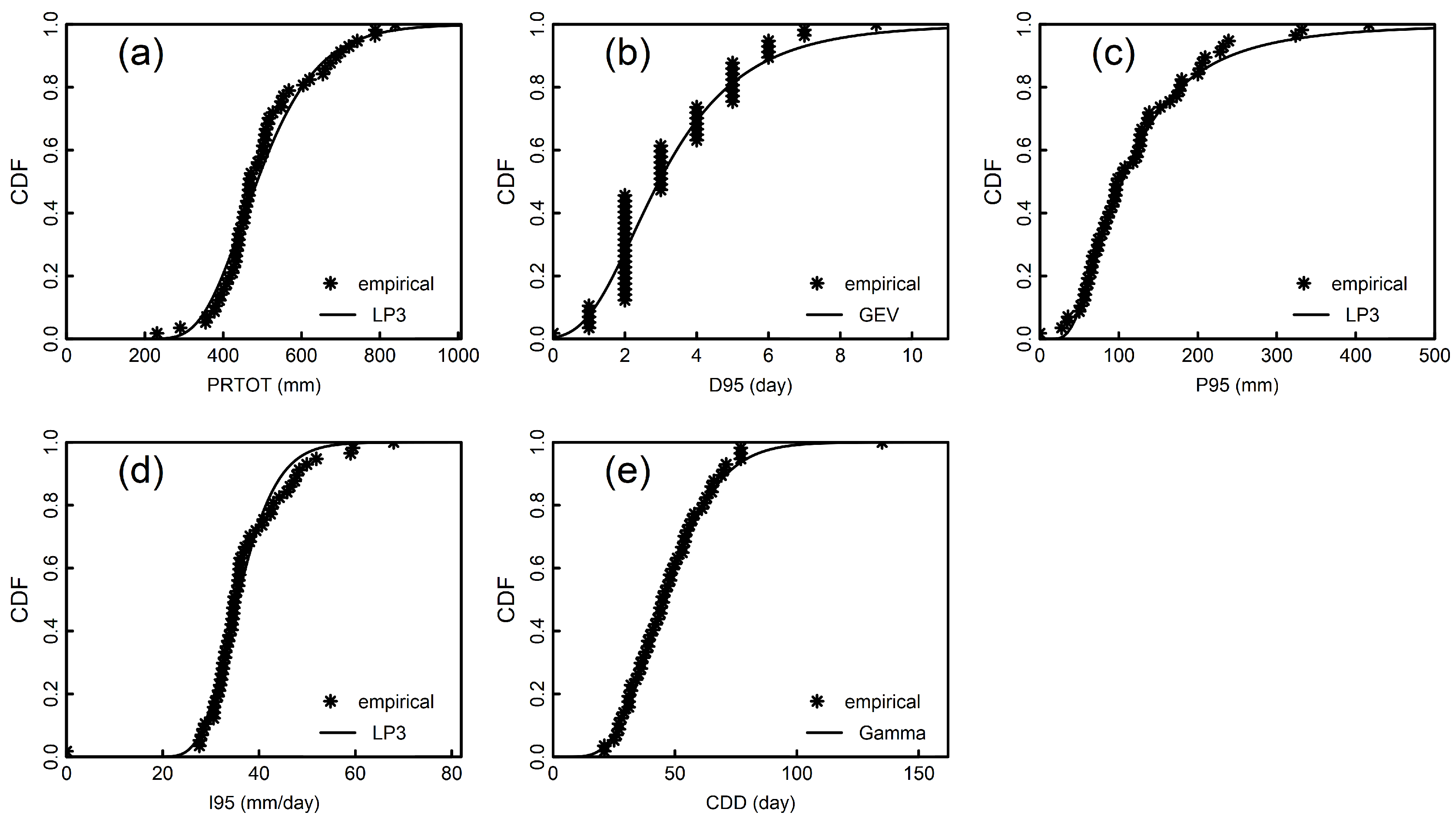
After calculating the results of the five selected precipitation indices for each station, the marginal distributions of those precipitation indices could be constructed. Taking Qindu station as an example, the best fitted marginal distributions for the five indices, including the parameter values of each fitted distribution, KS test results, RMSE, and AIC values are shown in Table 2. It can be seen from the table that PRTOT, P95, and D95 are all fitted by the LP III distribution, I95 is fitted with GEV distribution, and gamma distribution is more suitable for the CDD index. From the p values of KS test results, it can be concluded that all fitted distributions prove to be effective in describing the probabilistic features of the indicators (with p > 0.05). The graph-based verification method was used: Figure 2 compares the theoretical cumulative probability distribution to the empirical cumulative probability distribution for each indicator. This figure shows that the fitted CDF curves of the five indexes are very close to the observed values. For some indicators, we focused on the analysis of their upper tail performance (the top right end of the curve), such as I95, D95, P95, and CDD, because the closer the corresponding events of these indicators are to the upper tail end, the more serious these events are. PRTOT is a comprehensive evaluation index. The events close to the upper tail indicate that the annual precipitation is abundant, while the events close to the lower tail indicate that the annual precipitation is less. However, each fitting distribution performs well in the tail of interest, which shows that the risk inference results of extreme cases (high recurrence time period events) according to different indicators in the study are reliable.
Since the event with indicator at the upper tail (i.e., the event with indicator X > x) is located at the right tail of cumulative probability distribution, we marked it as the form of X_R. For the corresponding indices of I95, D95, P95, and CDD, they were marked as I95_R, D95_R, P95_R, and CDD_R, respectively. While, the events of the PRTOT indicator at the upper and lower tail (i.e., the events with index X ≤ x) were separately marked as PRTOT_R and PRTOT_L. After getting the fitted marginal distributions of all indices, the recurrence information of each indicator upon different tails can be obtained based on the Equation (3). Given the specific return period value, the corresponding indicator value can also be calculated. Taking the 10-year return period as an example, the values of the six indices for all stations corresponding to events of PRTOT_R, PRTOT_L, I95_R, D95_R, P95_R, and CDD_R were estimated.
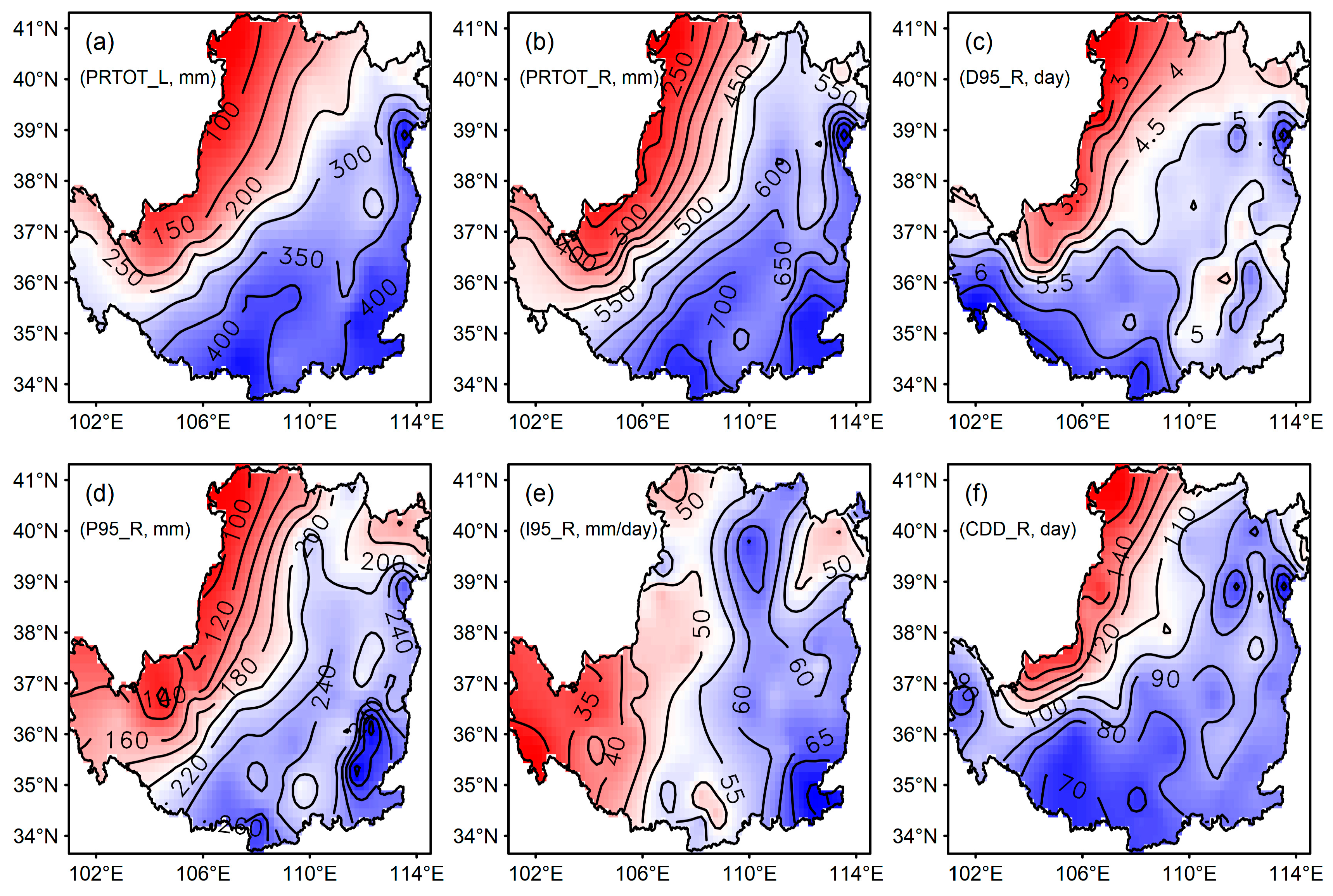
Figure 3 shows the computational results of six marked indices at 10-year return period over the Loess Plateau in the form of interpolation maps with contour lines. The color gradients were utilized to visually distinguish the differences of each indicator in different regions. Due to the spatial transition characteristics of precipitation over the Loess Plateau, Figure 3a–e shows a gradient increasing trend from northwest to southeast in the Loess Plateau, while Figure 3f (CDD_R) shows a gradient decreasing trend. The differences of 10-year return period values between PRTOT_R and PRTOT_L vary greatly, which shows a range of 127–373 mm at different stations and an average difference of 265 mm over the whole region. The PRTOT_R in the arid area can even reach 3.03 times higher than PRTOT_L. The comparison of P95_R and PRTOT_L shows that the extreme rainfall in wet year is only slightly lower than the annual precipitation in the dry year. The minimum value of I95_R appears in the high mountain area of the southwestern Loess Plateau, while in the northwest region with the least annual precipitation, the I95_R is merely slightly lower than the southeast region with the most precipitation. In addition, the value of D95_R in the northwest region is very low, which indicates that the annual precipitation in Northwest China may be highly concentrated in several heavy rainfall events and makes the region into severe drought for most of the year. This conclusion can also be obtained from the performance of CDD_R in this area, the duration of continuous drought of 10-year return period can even reach 160 days.
4.2. Bivariate Analysis
The combined events of X and Y are denoted as {X, Y} and {X or Y}, which, respectively, represents the concurrence of X and Y events, and the occurrence of X or Y event. The recurrence periods of the two combinations are labeled as T{X, Y} and T{X|Y}, respectively. For the five climate indicators, the joint performance of six combinations were studied, namely {PRTOT_L, CDD_R}, {PRTOT_R, CDD_R}, {D95_R, P95_R}, {P95_R, I95_R}, {P95_R or I95_R}, and {P95_R, CDD_R}. The definitions of joint RPs of precipitation indicators are listed in Table 3. T{PRTOT_L, CDD_R} indicates the joint return period of PRTOT less than and equal to a specific value and CDD exceed its specific threshold, which means a long period of continuous drought appears in a dry year. T{PRTOT_R, CDD_R} denotes the joint RP of long-term continuous drought occurs even when the annual precipitation is sufficient, indicating consecutive PRTOT and CDD exceed their specific thresholds simultaneously. {D95_R, P95_R} indicates a strong precipitation event with the precipitation amount and precipitation duration exceed their specific thresholds. {P95_R, I95_R}/T{P95_R|I95_R} signifies an extreme heavy precipitation event in which precipitation and/or precipitation intensity exceeds the thresholds. As a combination of extreme heavy precipitation and continuous drying indicators, {P95_R, CDD_R} implies the concurrence of floods and droughts in the same year.
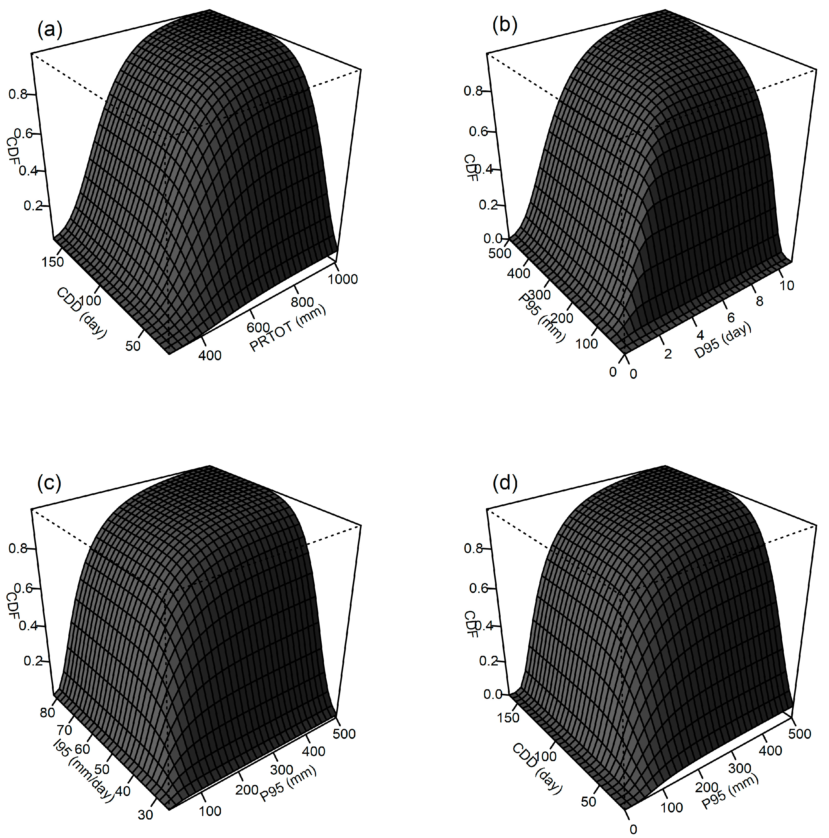
It can be seen from Table 3 that although joint RPs of six indicator combinations are going to be addressed, only the joint probability distributions of four combinations need to be quantified, namely {PRTOT, CDD}, {D95, P95}, {P95, I95}, and {P95, CDD} (see the last column). By using the best fitted marginal distribution functions, the joint probability distributions of four combinations can then be obtained by copulas. The KS test and the indices of RMSE, AIC were also applied to select the best performed copulas for different indicator combinations. Four bivariate CDF graphics based on the best fitted copulas at Qindu Station are presented in Figure 4. The numerical variation ranges of the two indicators for each combination is given on the x-axis and the y-axis, and the [0, 1] interval of the joint CDF is given on the z-axis.
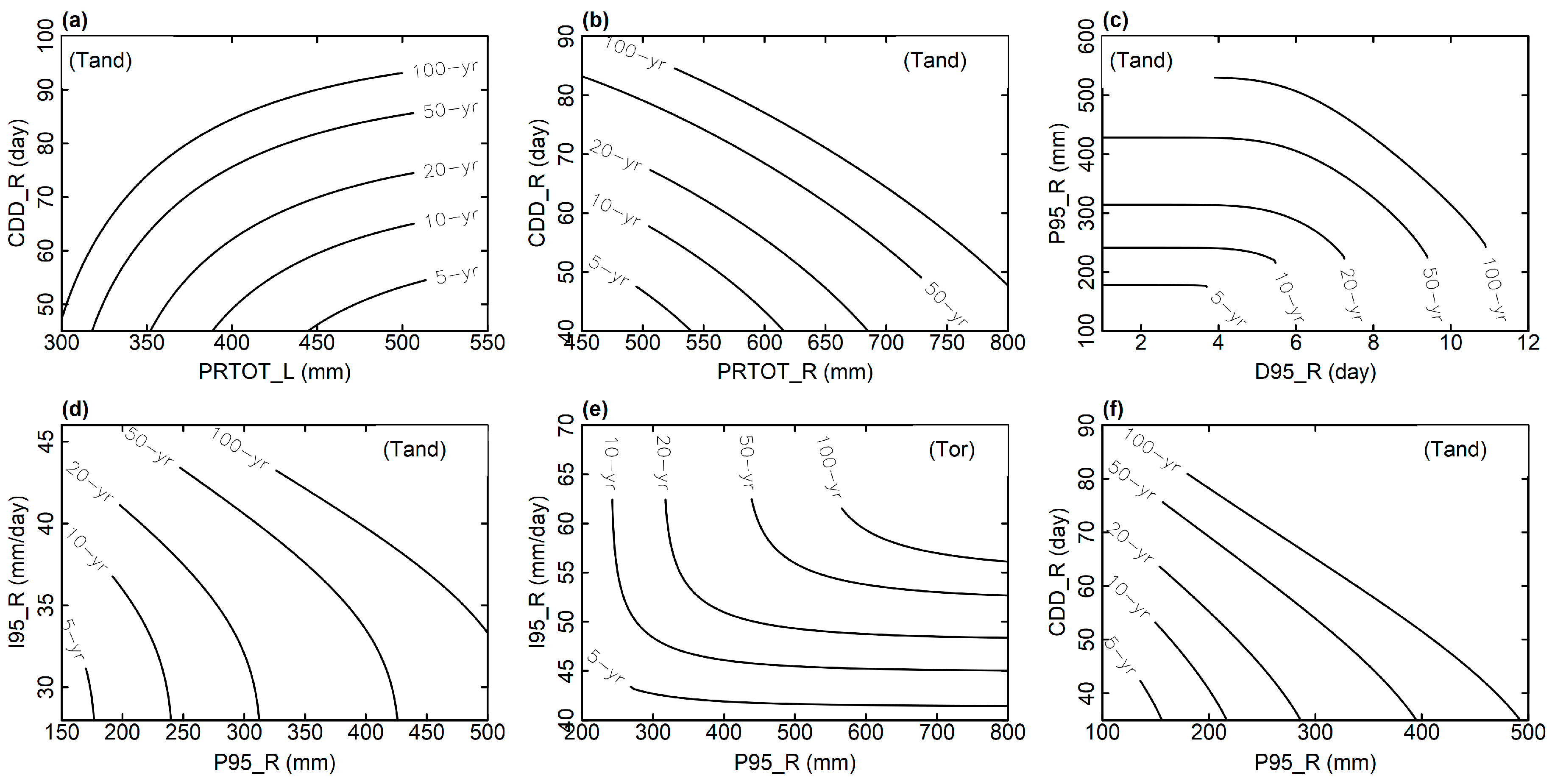
According to Equations (6)–(8), the value of return period is determined by two dependent variables, and thus it is possible to get the same return period value with different combinations of the variables. Figure 5 shows the contour maps of the joint return period of 5, 10, 20, 50, and 100 years under different combinations of six precipitation indicators. We can quantitatively reflect the joint risk of simultaneous occurrence of different precipitation extremes corresponding to their numerical combinations. Each index gradually tends to be less likely to occur along the direction of increasing joint return period, that is, the return period of single variable in this direction also gradually increases. It can be seen from the figure that the contour line of recurrence period presents three different forms: Figure 5a is obtained by Equation (8), and the joint recurrence period gradually increases in the direction in which the PRTOT tends to the lower tail and the CDD tends to the upper tail. Figure 5b–d, f is achieved through Equation (6) and the joint RP of each group would gradually increase in the direction of the upward tail of both variables. Figure 5e is obtained from Equation (7). Compared with Figure 4, it can be seen that for two climate indicators with same numerical combination, Figure 5e always shows a smaller return period, that is, the events with relationship of ‘or’ is more likely to occur.
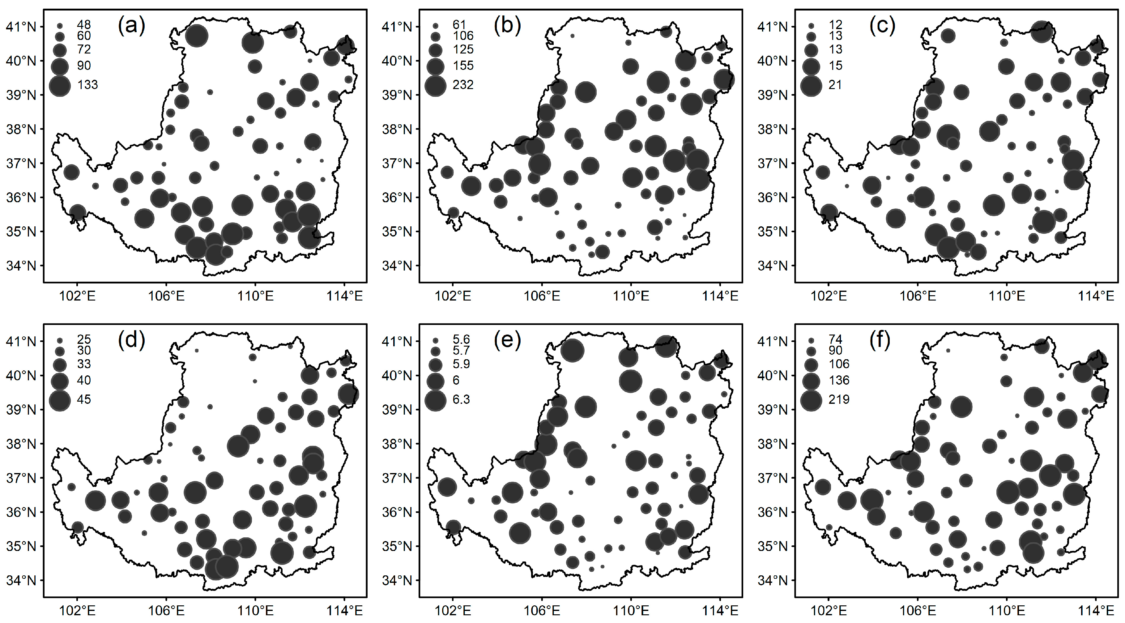
Figure 6 shows the joint RPs of each combination group under the condition of given 10-year return periods for two single indicators (corresponding to Figure 3). Figure 6a–f, respectively, denotes the six combinations of ID1–ID6 in Table 3 and the values of the recurrence periods vary directly proportional to the size of the solid circles in the figure. By comparing the joint return periods of Figure 6a with Figure 6b, it can be seen that the return period values of Figure 6b are always larger (58.5 years larger on average) than that of Figure 6a. The results of the study area as a whole are consistent with our general perception that wet years are less prone to prolonged continuous drought. It is worth noticing that there are still 17 stations with T{PRTOT_L, CDD_R} larger than T{PRTOT_R, CDD_R}. This is because the annual precipitation of these stations is more concentrated in few extreme precipitation events, and CDD is less affected by the annual precipitation, and thus the two precipitation indicators even show a certain degree of negative correlation.
From the spatial distribution of RPs, the size of the circles in Figure 6a,b in the whole region is basically opposite, which means that the events of {PRTOT_L, CDD_R} have difficulty occurring at the stations where the events of {PRTOT_R, CDD_R} are relatively easy to occur. The spatial distribution of circles of different sizes in Figure 6f is similar to that in Figure 6b, that is, the events of {PRTOT_R, CDD_R} and {P95_R, CDD_R} show some degree of convergence. This is because the annual precipitation for this condition is too concentrated. Figure 6c–e shows the joint return periods of different combinations of the three extreme heavy precipitation indicators. The corresponding joint return periods are all relatively smaller than other combinations, which is because the three indicators are strongly correlated.
The average return periods of all stations in Figure 6a,b,f are 85.2, 143.8, and 126.2, respectively. These results demonstrate that the three compound events with two indicators corresponding to the 10-year return period have difficulty occurring simultaneously in the same year. However, the quantitative calculation results are greatly affected by the selection of different models since the joint probabilities of these events are very close to the tails, which suggest that the quantitative results will show great uncertainty. Correspondingly, the joint RP values of Figure 6c–e are too small to exhibit their extreme risk situations, especially for Figure 6c,e. This requires a balance that allows the assessment to calculate the degree of extreme risk that may occur within its credible return periods. As the time series of precipitation data used in this paper is about 60 years, the return period of individual extreme indicators with a joint RP of 50 years corresponding to Figure 6c–e are considered to be calculated. Under the condition of two univariate return period values are set to be equal to each other, by using Equations (9)–(11), and then the specific values for each individual indicator (Figure 7) and the corresponding return periods (Figure 8) are obtained.
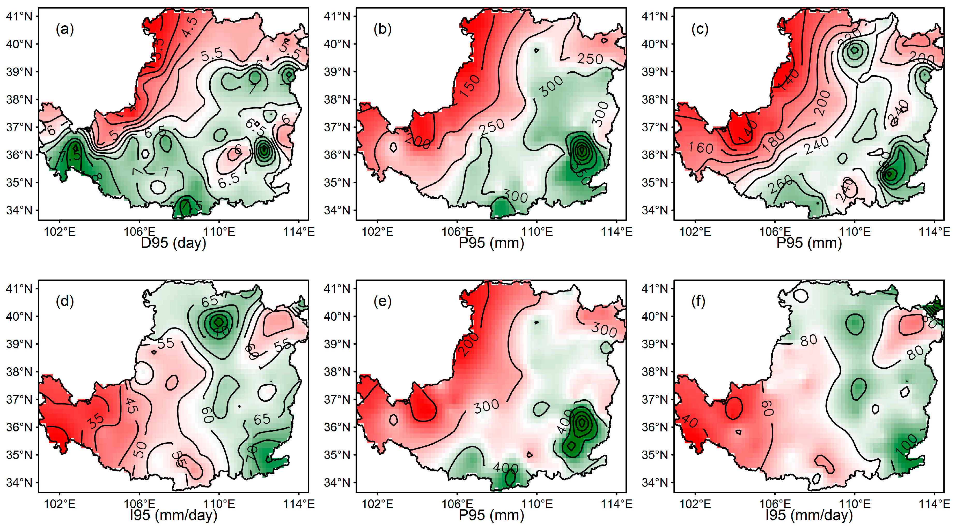
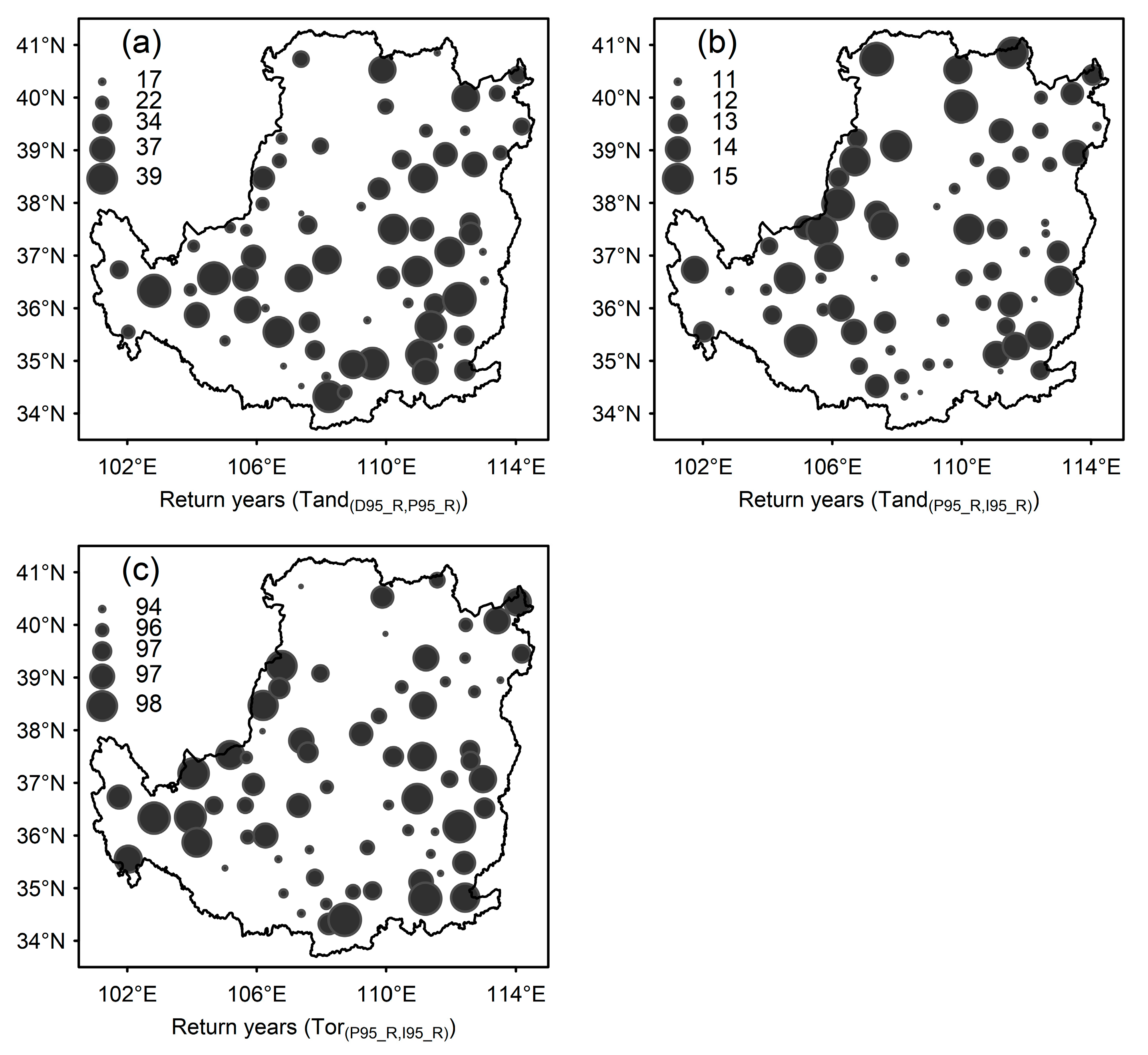
Figure 7a,b are individually, the interpolation maps of D95 and P95 with the joint return period of 50 years for events of {D95_R, P95_R}. The results show that spatial distribution of the two indicators is very similar to each other, and the overall values are higher than the values of the 10-year return period in Figure 3. The corresponding return period of single variable ranges from 15.7 to 44.4 years, with an average of 29.1 years (Figure 8a). Similarly, Figure 7c,d and Figure 8b and Figure 7e,f and Figure 8c show the respective indicator values in the events of {P95_R, I95_R} and {P95_R or I95_R}, respectively. It can be seen that the indicator values of {P95_R or I95_R} events are much higher than those of {P95_R, I95_R} events, in which the P95 is 112.3 mm higher on average, and I95 is 19.9 mm/day higher on average. The return periods of P95_R and I95_R in events of {P95_R or I95_R} are close to 100 year. In terms of probability, the 100-year RP of the P95 event or the 100-year RP of the I95 event can be encountered in 50 years. Heavy rainfall events are especially serious in the south and northeast of the Loess Plateau. The station with the most amount of extreme heavy rainfall shows a P95 of 931 mm, and the I95 is 97 mm/day.
5. Conclusions and Discussion
Based on the daily precipitation data of past six decades, the probability characteristics of five extreme precipitation indices in the Loess Plateau were studied. Moreover, the joint risk of different combinations of precipitation indexes was quantitatively evaluated. Specifically, six marginal distribution functions were applied to fit each precipitation index and six copula models belonging to the elliptic copula and Archimedes copula family were selected to fit the joint distributions of six indicator combinations. The RMSE, AIC, KS tests were used to evaluate the performance of marginal and joint distributions. The index values corresponding to the 10-year return period of each precipitation indicator were calculated, and the joint return periods of all combinations under the condition of 10-year return period for single variables were calculated. Finally, the indicator values with their RPs of three extreme heavy precipitation index combinations were calculated under the condition of a 50-year joint return period.
Main findings of the present study are summarized as follows: the study of single indicators shows that the extreme precipitation in wet years is almost equal to the annual precipitation in dry years over the Loess Plateau. The Northwest Loess Plateau with least amount of annual precipitation shows extreme precipitation intensity is only slightly lower than that in the humid southwest area. It is also found that the T{PRTOT_L, CDD_R} is greater than T{PRTOT_R, CDD_R} at 17 stations, which is also because the precipitation of these stations is mostly concentrated in a few extreme precipitation events, while CDD is less affected by the annual precipitation, and the two precipitation indicators even show a certain degree of negative correlation. In terms of probability, a P95 or I95 event of 100-year level can be encountered in a 50-year return period over the Loess Plateau. The precipitation amount and intensity of the Loess Plateau vary greatly in spatial distribution. The 10-year return period in the northwestern region can occur for more than five months with no precipitation events. In the southeastern region, there are foreseeable long-term extreme precipitation events.
Previous studies on the risk assessment of extreme precipitation often ignored the correlated characteristics of different precipitation indicators and could not quantitatively evaluate the joint risk of different indicators. Few studies have analyzed the joint risks of different indicators, however they are all aimed at the forward calculation process, that is, by giving fixed indicator values of certain recurrence periods to calculate the joint return period. The disadvantage of this scheme is that the obtained joint return periods always tend to be too small or too large. Too small a recurrence period does not reflect the severity of the event, and too large a recurrence period means that event is very close to the tail of the distribution and the result is unreliable. In this study, the univariate and joint risks of different extreme precipitation indexes in the Loess Plateau were synthetically studied by forward and reverse calculations, and the RPs of univariate indicators based on joint RPs of 50 years were calculated.
The Loess Plateau is located on the edge of different climatic regions, which results in the serious imbalance of the spatial and temporal distribution of precipitation. The annual precipitation is highly concentrated in rainy seasons, which makes the region in a serious drought state for most of the year, especially for the northwest region, while the Southwest Loess Plateau is prone to very heavy rainfall. Therefore, it is necessary to develop an effective management plan for water resources systems and environments. A systematic plan for water storage in flood seasons and water resources allocation in dry seasons is essentially needed.
Author Contributions
Conceptualization, C.S.; methodology, C.S. and Y.F.; software, C.S.; validation, Y.F., and C.S.; formal analysis, C.S.; investigation, C.S.; resources, G.H.; data curation, C.S.; writing—original draft preparation, C.S.; writing—review and editing, Y.F. and G.H.; visualization, C.S.; supervision, G.H.; project administration, G.H.; funding acquisition, G.H. All authors have read and agreed to the published version of the manuscript.
Funding
This research was supported by the National Key Research and Development Plan (2016YFA0601502), the Natural Sciences Foundation (51520105013, 51679087), the 111 Program (B14008), the Natural Science and Engineering Research Council of Canada, and the Fundamental Research Funds for the Central Universities (2016XS89).
Conflicts of Interest
The authors declare no conflict of interest.
References
- Climate Change 2007: The Physical Science Basis; Contribution of Working Group I to the Fourth Assessment Report of the Intergovernmental Panel on Climate Change; Cambridge University Press: Cambridge, UK, 2007.
- Climate Change 2014: Impacts, Adaptation, and Vulnerability; Contribution to the Fifth Assessment Report of the Intergovernmental Panel on Climate Change; Cambridge University Press: Cambridge, UK, 2014.
- Emori, S. Dynamic and thermodynamic changes in mean and extreme precipitation under changed climate. Geophys. Res. Lett. 2005, 32, L17706. [Google Scholar] [CrossRef]
- Barros, V.; Stocker, T.F. Managing the risks of extreme events and disasters to advance climate change adaptation: Special report of the Intergovernmental Panel on Climate Change. J. Clin. Microbiol. Metab. 2012, 18, 586–599. [Google Scholar]
- Lu, W.; Qin, X.; Jun, C. A parsimonious framework of evaluating WSUD features in urban flood mitigation. J. Environ. Inf. 2019, 33, 17–27. [Google Scholar] [CrossRef]
- Chang, L.-C.; Chang, F.-J. Intelligent control for modelling of real-time reservoir operation. Hydrol. Process. 2010, 15, 1621–1634. [Google Scholar] [CrossRef]
- Jhong, B.C.; Tung, C.P. Evaluating future joint probability of precipitation extremes with a copula-based assessing approach in climate change. Water Resour. Manag. 2018, 32, 4253–4274. [Google Scholar] [CrossRef]
- Kharin, V.V.; Zwiers, F.W.; Zhang, X.; Wehner, M. Changes in temperature and precipitation extremes in the CMIP5 ensemble. Clim. Chang. 2013, 119, 345–357. [Google Scholar] [CrossRef]
- Caesar, J.; Alexander, L.V.; Trewin, B.; Tse-ring, K.; Sorany, L.; Vuniyayawa, V.; Keosavang, N.; Shimana, A.; Htay, M.M.; Karmacharya, J.; et al. Changes in temperature and precipitation extremes over the Indo-Pacific region from 1971 to 2005. Int. J. Climatol. 2011, 31, 791–801. [Google Scholar] [CrossRef]
- You, Q.; Kang, S.; Aguilar, E.; Pepin, N.; Flügel, W.-A.; Yan, Y. Changes in daily climate extremes in China and their connection to the large scale atmospheric circulation during 1961–2003. Clim. Dyn. 2011, 36, 2399–2417. [Google Scholar] [CrossRef]
- Zhai, P.; Zhang, X.; Wan, H.; Pan, X. Trends in total precipitation and frequency of daily precipitation extremes over China. J. Clim. 2005, 18, 1096–1108. [Google Scholar] [CrossRef]
- Wang, C.; Ren, X.; Li, Y. Analysis of extreme precipitation characteristics in low mountain areas based on three-dimensional copulas—Taking Kuandian County as an example. Theo. Appl. Climato. 2017, 128, 169–179. [Google Scholar] [CrossRef]
- Wahl, T.; Jain, S.; Bender, J.; Meyers, S.D.; Luther, M.E. Increasing risk of compound flooding from storm surge and rainfall for major us cities. Nat. Clim. Chang. 2015, 5, 1093–1097. [Google Scholar] [CrossRef]
- Madadgar, S.; Aghakouchak, A.; Farahmand, A.; Davis, S.J. Probabilistic estimates of drought impacts on agricultural production. Geophys. Res. Lett. 2017, 44, 7799–7807. [Google Scholar] [CrossRef]
- Zhang, D.D.; Yan, D.H.; Lu, F.; Wang, Y.C.; Feng, J. Copula-based risk assessment of drought in Yunnan province, China. Nat. Hazards 2015, 75, 2199–2220. [Google Scholar] [CrossRef]
- Rana, A.; Moradkhani, H.; Qin, Y. Understanding the joint behavior of temperature and precipitation for climate change impact studies. Theo. Appl. Clim. 2016, 129, 1–19. [Google Scholar] [CrossRef]
- Jeong, D.I.; Sushama, L.; Khaliq, M.N.; René, R. A copula-based multivariate analysis of canadian rcm projected changes to flood characteristics for northeastern Canada. Clim. Dyn. 2014, 42, 2045–2066. [Google Scholar] [CrossRef] [Green Version]
- Qian, L.; Wang, H.; Dang, S.; Wang, C.; Jiao, Z.; Zhao, Y. Modelling bivariate extreme precipitation distribution for data-scarce regions using gumbel-hougaard copula with maximum entropy estimation. Hydrol. Process. 2017, 32, 212–227. [Google Scholar] [CrossRef]
- Salvadori, G.; De Michele, C. Multivariate real-time assessment of droughts via copula-based multi-site hazard trajectories and fans. J. Hydrol. 2015, 526, 101–115. [Google Scholar] [CrossRef]
- Volpi, E.; Fiori, A. Hydraulic structures subject to bivariate hydrological loads: Return period, design, and risk assessment. Water Resour. Res. 2014, 50, 885–897. [Google Scholar] [CrossRef]
- Fan, Y.R.; Huang, W.W.; Huang, G.H.; Huang, K.; Li, Y.P.; Kong, X.M. Bivariate hydrologic risk analysis based on a coupled entropy-copula method for the Xiangxi River in the Three Gorges Reservoir area, China. Theor. Appl. Clim. 2016, 125, 381–397. [Google Scholar] [CrossRef]
- Zhang, Q.; Li, J.; Singh, V.P.; Xu, C.Y. Copula-based spatio-temporal patterns of precipitation extremes in China. Int. J. Clim. 2013, 33, 1140–1152. [Google Scholar] [CrossRef]
- Goswami, U.P.; Hazra, B.; Kumar, G.M. Copula-based probabilistic characterization of precipitation extremes over north sikkim himalaya. Atmos. Res. 2018, 212, 273–284. [Google Scholar] [CrossRef]
- Wang, L.; Cheung, K.K.W.; Chi-Yung, T.; Tai, A.P.K.; Li, Y. Evaluation of the regional climate model over the loess plateau of China. Int. J. Climatol. 2018, 38, 35–54. [Google Scholar] [CrossRef]
- Xin, Z.; Yu, X.; Li, Q.; Lu, X.X. Spatiotemporal variation in rainfall erosivity on the Chinese loess plateau during the period 1956–2008. Regional Environ. Chang. 2011, 11, 149–159. [Google Scholar] [CrossRef]
- Liu, Q.; Yang, Z. Quantitative estimation of the impact of climate change on actual evapotranspiration in the yellow river basin, China. J. Hydrol. 2010, 395, 226–234. [Google Scholar] [CrossRef]
- Li, Z.; Zheng, F.L.; Liu, W.Z.; Jiang, D.J. Spatially downscaling gcms outputs to project changes in extreme precipitation and temperature events on the loess plateau of China during the 21st century. Global Planet. Chang. 2012, 82, 0–73. [Google Scholar] [CrossRef]
- Nolan, S.; Unkovich, M.; Yuying, S.; Lingling, L.; Bellotti, W. Farming systems of the loess plateau, Gansu province, China. Agric. Ecosyst. Environ. 2008, 124, 13–23. [Google Scholar] [CrossRef]
- Liang, W.; Bai, D.; Wang, F.; Fu, B.; Yan, J.; Wang, S.; Yang, Y.; Long, D.; Feng, M. Quantifying the impacts of climate change and ecological restoration on streamflow changes based on a budyko hydrological model in China’s Loess Plateau. Water Resour. Res. 2015, 51, 6500–6519. [Google Scholar] [CrossRef]
- Wang, X.L. Accounting for autocorrelation in detecting mean shifts in climate data series using the penalized maximal t or f test. J. Appl. Meteorol. Climatol. 2008, 47, 2423–2444. [Google Scholar] [CrossRef]
- Wang, W.; Shao, Q.; Peng, S.; Zhang, Z.; Xing, W.; An, G.; Yong, B. Spatial and temporal characteristics of changes in precipitation during 1957–2007 in the haihe river basin, China. Stochastic Environ. Res. Risk Assess. 2011, 25, 881–895. [Google Scholar] [CrossRef]
- Sun, C.X.; Huang, G.H.; Fan, Y.; Zhou, X.; Lu, C.; Wang, X.Q. Drought occurring with hot extremes: Changes under future climate change on Loess Plateau, China. Earth’s Future 2019, 7, 587–604. [Google Scholar] [CrossRef] [Green Version]
- Akaike, H. A new look at the statistical model identification. IEEE Trans. Autom. Control. 1974, 19, 716–723. [Google Scholar] [CrossRef]
- Gringorten, I.I. A plotting rule for extreme probability paper. J. Geophys. Res. 1963, 68, 813–814. [Google Scholar] [CrossRef]
- Sklar, K. Fonctions dé repartition á n dimensions et leurs marges. Publications de l’Institut de Statistique de l’Universite dé Paris 1959, 8, 229–231. [Google Scholar]
- Nelsen, R.B. An Introduction to Copulas; Springer: New York, NY, USA, 2006. [Google Scholar]
- Sraj, M.; Bezak, N.; Brilly, M. Bivariate flood frequency analysis using the copula function: A case study of the litija station on the sava river. Hydrol. Process. 2015, 29, 225–238. [Google Scholar] [CrossRef]
- Zhou, X.; Huang, G.; Wang, X.; Fan, Y.; Cheng, G. A coupled dynamical-copula downscaling approach for temperature projections over the canadian prairies. Clim. Dyn. 2018, 51, 2413–2431. [Google Scholar] [CrossRef]
- Salvadori, G.; de Michele, C. Frequency analysis via copulas: Theoretical aspects and applications to hydrological events. Water Resour. Res. 2004, 40, 1–17. [Google Scholar] [CrossRef]
- Egrioglu, E.; Aladag, C.; Basaran, M. A new approach based on the optimization of the length of intervals in fuzzy time series. J. Intell. Fuzzy Syst. 2011, 22, 15–19. [Google Scholar] [CrossRef]
- Bürger, G.; Murdock, T.Q.; Werner, A.T.; Sobie, S.R.; Cannon, A.J. Downscaling Extremes—An Intercomparison of Multiple Statistical Methods for Present Climate. J. Clim. 2012, 2, 4366–4388. [Google Scholar]
- Shivam, G.; Goyal, M.K.; Sarma, A.K. Index-based study of future precipitation changes over subansiri river catchment under changing climate. J. Environ. Inf. 2019, 34, 1–14. [Google Scholar] [CrossRef]
Figure 1.
Geographical location and 69 meteorological stations of the Loess Plateau.

Figure 2.
Comparison of the empirical distributions and best fitting distributions for five precipitation indices in Qindu station: (a) PRTOT, (b) D95, (c) P95, (d) I95, and (e) CDD.
Figure 2.
Comparison of the empirical distributions and best fitting distributions for five precipitation indices in Qindu station: (a) PRTOT, (b) D95, (c) P95, (d) I95, and (e) CDD.

Figure 3.
The values of six marked indexes at 10-year return period over the the Loess Plateau: (a) PRTOT_L, (b) PRTOT_R, (c) D95_R, (d) P95_R, (e) I95_R, and (f) CDD_R.
Figure 3.
The values of six marked indexes at 10-year return period over the the Loess Plateau: (a) PRTOT_L, (b) PRTOT_R, (c) D95_R, (d) P95_R, (e) I95_R, and (f) CDD_R.

Figure 4.
Joint cumulative distribution functions (CDFs) based on the best fitted copulas for four indicator combinations at Qindu Station: (a) {PRTOT, CDD}, (b) {D95, P95}, (c) {P95, I95}, and (d) {P95, CDD}.
Figure 4.
Joint cumulative distribution functions (CDFs) based on the best fitted copulas for four indicator combinations at Qindu Station: (a) {PRTOT, CDD}, (b) {D95, P95}, (c) {P95, I95}, and (d) {P95, CDD}.

Figure 5.
The joint return period of 5, 10, 20, 50, and 100 years under different combinations of six climate indicators: (a) “And” relation for combination of {PRTOT_L, CDD_R}, (b) “And” relation for combination of {PRTOT_R, CDD_R}, (c) “And” relation for combination of {D95_R, P95_R}, (d)“And” relation for combination of {P95_R, I95_R}, (e) “Or” relation for combination of {P95_R, I95_R}, and (f) “And” relation for combination of {P95_R, CDD_R}.

Figure 6.
The joint returns periods of each combination group under the condition of 10-year return periods of two single indicators. (a–e) Represent six combinations of events: {PRTOT_L, CDD_R}, {PRTOT_R, CDD_R}, {D95_R, P95_R}, {P95_R, I95_R}, {P95_R or I95_R}, and {P95_R, CDD_R}.
Figure 6.
The joint returns periods of each combination group under the condition of 10-year return periods of two single indicators. (a–e) Represent six combinations of events: {PRTOT_L, CDD_R}, {PRTOT_R, CDD_R}, {D95_R, P95_R}, {P95_R, I95_R}, {P95_R or I95_R}, and {P95_R, CDD_R}.

Figure 7.
The specific values for each individual indicator under joint return period of 50 years corresponding to three combination groups: (a) and (b) correspond to the {D95_R, P95_R} event; (c) and (d) correspond to the {P95_R, I95_R} event; (e) and (f) correspond to the {P95_R or I95_R} event.
Figure 7.
The specific values for each individual indicator under joint return period of 50 years corresponding to three combination groups: (a) and (b) correspond to the {D95_R, P95_R} event; (c) and (d) correspond to the {P95_R, I95_R} event; (e) and (f) correspond to the {P95_R or I95_R} event.

Figure 8.
The univariate return period values for each individual indicator under joint return period of 50 years corresponding to three combination groups: (a) corresponds to the {D95_R, P95_R} event; (b) corresponds to the {P95_R, I95_R} event; (c) corresponds to the {P95_R or I95_R} event.
Figure 8.
The univariate return period values for each individual indicator under joint return period of 50 years corresponding to three combination groups: (a) corresponds to the {D95_R, P95_R} event; (b) corresponds to the {P95_R, I95_R} event; (c) corresponds to the {P95_R or I95_R} event.


Table 1.
Definitions of five precipitation indices that were used in the study.
| Indices | Abbreviations | Definitions | Unit |
|---|---|---|---|
| PRTOT | PRTOT | The amount of annual total precipitation | mm |
| Number of extreme heavy precipitation days | D95 | Number of days with precipitation exceeding the 95th percentile of precipitation series (daily precipitation ≥1 mm) during 1971–2000. | days |
| The amount of extreme heavy precipitation | P95 | Annual total amount of precipitation with daily precipitation exceeding the 95th percentile of precipitation series during 1971–2000 | mm |
| The intensity of extreme heavy precipitation | I95 | Mean daily precipitation intensity of extreme heavy precipitation | mm/day |
| Consecutive dry days | CDD | Maximum number of consecutive dry days (days with precipitation <1 mm) | days |
Table 2.
Statistical test results for marginal distribution of five precipitation indices of Qindu station.
Table 2.
Statistical test results for marginal distribution of five precipitation indices of Qindu station.
| Indices | Marginal Distribution | a | b | α | K-S Test | RMSE | AIC | |
|---|---|---|---|---|---|---|---|---|
| T | p value | |||||||
| PRTOT | LP III | 118.81 | 44.46 | 3.52 | 0.10 | 0.63 | 0.0458 | −339.14 |
| D95 | GEV | 0.11 | 1.52 | 2.38 | 0.17 | 0.10 | 0.0655 | −299.34 |
| P95 | LP III | 26.73 | 8.47 | 1.53 | 0.05 | 0.99 | 0.0194 | −435.49 |
| I95 | LP III | 163.79 | 72.20 | 1.31 | 0.11 | 0.53 | 0.0485 | −332.81 |
| CDD | Gamma | 7.59 | 0.16 | 0.05 | 0.99 | 0.0521 | −471.51 | |
Notes: parameters of marginal distribution functions: for LP III and GEV distributions, a, b, and α represent the shape, scale, and location parameter, respectively; For Gamma distribution, a and b indicate the shape and rate parameter, respectively.
Table 3.
The indicator combinations with their definitions.
| ID | Combinations | Return Periods (years) | Variables (X, Y) |
|---|---|---|---|
| 1 | {PRTOT_L, CDD_R} | T{X ≤ x and Y > y} | PRTOT, CDD |
| 2 | {PRTOT_R, CDD_R} | T{X > x and Y > y} | PRTOT, CDD |
| 3 | {D95_R, P95_R} | T{X > x and Y > y} | D95, P95 |
| 4 | {P95_R, I95_R} | T{X > x and Y > y} | P95, I95 |
| 5 | {P95_R or I95_R} | T{X > x or Y > y} | P95, I95 |
| 6 | {P95_R, CDD_R} | T{X > x and Y > y} | P95, CDD |
© 2020 by the authors. Licensee MDPI, Basel, Switzerland. This article is an open access article distributed under the terms and conditions of the Creative Commons Attribution (CC BY) license (http://creativecommons.org/licenses/by/4.0/).
Share and Cite
MDPI and ACS Style
Sun, C.; Huang, G.; Fan, Y. Multi-Indicator Evaluation for Extreme Precipitation Events in the Past 60 Years over the Loess Plateau. Water 2020, 12, 193. https://doi.org/10.3390/w12010193
AMA Style
Sun C, Huang G, Fan Y. Multi-Indicator Evaluation for Extreme Precipitation Events in the Past 60 Years over the Loess Plateau. Water. 2020; 12(1):193. https://doi.org/10.3390/w12010193
Chicago/Turabian StyleSun, Chaoxing, Guohe Huang, and Yurui Fan. 2020. "Multi-Indicator Evaluation for Extreme Precipitation Events in the Past 60 Years over the Loess Plateau" Water 12, no. 1: 193. https://doi.org/10.3390/w12010193
Note that from the first issue of 2016, this journal uses article numbers instead of page numbers. See further details here.