Estimation of Annual Maximum and Minimum Flow Trends in a Data-Scarce Basin. Case Study of the Allipén River Watershed, Chile

1
Department of Civil Engineering, Universidad Católica de la Santísima Concepción, Concepción 4090541, Chile
2
Centro de Investigación en Biodiversidad y Ambientes Sustentables (CIBAS), Universidad Católica de la Santísima Concepción, Concepción 4090541, Chile
*
Author to whom correspondence should be addressed.
Water 2020, 12(1), 162; https://doi.org/10.3390/w12010162
Submission received: 28 November 2019
/
Revised: 28 December 2019
/
Accepted: 1 January 2020
/
Published: 5 January 2020
(This article belongs to the Special Issue Management of Hydrological Extremes: Floods and Droughts)
Abstract
:Data on historical extreme events provides information not only for water resources planning and management but also for the design of disaster-prevention measures. However, most basins around the globe lack long-term hydro-meteorological information to derive the trend of hydrological extremes. This study aims to investigate a method to estimate maximum and minimum flow trends in basins with limited streamflow records. To carry out this study, data from the Allipén River watershed (Chile), the Hydrologiska Byråns Vattenbalansavdelning (HBV) hydrological model at a daily time step, and an uncertainty analysis were used. Through a calibration using only five years of records, 21-year mean daily flow series were generated and the extreme values derived. To analyze the effect of the length of data availability, 2, 5, and 10 years of flows were eliminated from the analyses. The results show that in the case of 11 years of simulated flows, the annual maximum and minimum flow trends present greater uncertainty than in the cases of 16 and 19 years of simulated flows. Simulating 16 years, however, proved to properly simulate the observed long-term trends. Therefore, in data-scarce areas, the use of a hydrological model to simulate extreme mean daily flows and estimate long-term trends with at least 16 years of meteorological data could be a valid option.
1. Introduction
Water availability changes each year due to local, global, natural, and anthropogenic phenomena. These changes and the constant increase in demand, be it for human consumption, irrigation, hydropower, or industrial use, require increasingly efficient water resources planning and management [1]. Moreover, the frequency and magnitude of extreme meteorological events, such as floods and droughts are currently changing [2,3]. Despite scientific and technological progress, the population remains exposed to these events [4]; therefore, trend analysis of hydroclimatic variables has become the study focus for many researchers around the world [3,5,6].
Several studies have shown that changes in flow time series are due to climatic [7,8,9,10] and/or anthropogenic factors [11,12,13]. To analyze the hydrological behavior in a watershed it is important to determine maximum and minimum flow trends; however, ascertaining the history of a basin can be a difficult task when the available hydrometeorological information is limited [14]. Most drainage basins around the globe are ungauged or data-scarce, either because a required variable has not been sampled at the required resolution or because it has not been observed during a period of interest [15]. To address this limitation, different approaches have been developed to estimate stream flows in ungauged areas [16], for example, multiple linear regression (MLR), variations of autoregressive moving-average (ARMA) models, artificial neural networks (ANNs) [17,18], and the widely used conceptual or physically-based hydrological models.
Currently, hydrological models are important components in planning and management of water resources, since they allow the simulation of streamflow series through a simplified representation of hydrological processes. There are various hydrological models, which vary in complexity and utility [19]. Most hydrological models can be classified as conceptual models, with parameters, or at least some parameters, that cannot be directly physically interpreted or measured, making it necessary to estimate them through a calibration process [20,21]. These models can be lumped, semi-distributed, or distributed. Depending on the aim of the study and information availability, lumped models may be preferred, since they provide acceptable results in terms of accuracy [22] and are simpler to interpret and implement than distributed models, especially in scarce-data cases.
In recent years, several studies have reported a decrease in precipitation and in snow and glacier coverage [23,24,25,26,27,28,29] and increasing temperature trends [30,31] in south-central Chile. These changes might affect the way in which water is managed on a regional scale, as well as how extreme events, such as floods and droughts, are faced.
Several countries around the globe currently need to face the lack of hydrological data for water-related management and planning. In Chile, streamflow records have a relatively short length of 30 years on average [32], and gauging stations are unevenly distributed throughout the country [33], limiting basin-and regional-scale analysis of flow trends and making it difficult to study runoff changes [34,35].
Time series reconstruction using a dendroclimatological approach [36,37,38,39,40,41] has been one of the most used methods to conduct hydrological long-term trends analyses. Tree-ring records provide continuous series of past environmental changes for the last several centuries and in some cases, millennia [36]. However, there is still a lack of specific studies related to the analysis of extreme flow trends and, more importantly, such trends in basins with limited hydrological information. Several studies used extensive databases [42,43,44,45] and performed a data quality control considering criteria such as no gaps and a length of time-series of at least 40–50 years. Thus, the objective of this article is to investigate a method to estimate such hydrological extreme trends, with a controlled and known uncertainty, in a basin with limited data availability. With this aim, a combined approach of hydrological modeling with a calibration using 5-years of data, a short simulation window (up to 21 years), and uncertainty analysis of flow trends is used.
2. Study Area and Data
2.1. Study Area
The Allipén River watershed was chosen as a case study location. The Allipén River watershed until the Río Allipén en Los Laureles stream-gauge station (1652 km2) is located in southern Chile and monitored by the Chilean General Water Directorate (DGA; Figure 1). The Allipén River rises in the Andes Mountains. Its climate varies between warm, temperate and rainy in the middle and lower parts of the watershed to cold, temperate and rainy with Mediterranean influence in its upper part (the Andean area). Annual precipitation can reach 3000 mm and mean monthly temperatures oscillate between −3 and 18 °C. The watershed receives mostly pluvial precipitation, with slight snow influence in the upper part, presenting a mixed hydrological regime (pluvio-nival). In the upper watershed volcano-sedimentary rock formations of the Tertiary and Quaternary periods are prominent, while in the Central Valley there are unconsolidated deposits of glacial origin and highly permeable alluvial material [46].
2.2. Data
To implement the hydrological model of the watershed, mean daily precipitation, temperature, and monthly evapotranspiration series representative of the watershed are required. The Los Laureles, Quecheregua, Cunco, Cherquenco, Tricauco, and Malalcahuello rain gauge stations (see locations in Figure 1), managed by the DGA, were used. To estimate mean precipitation in the watershed, the inverse distance weighting (IDW) method was used. Due to the absence of temperature records, 0.25°—resolution (~25 km) gridded data series published by the Department of Civil and Environmental Engineering of Princeton University [47] were obtained and the Thiessen Polygon method was used to interpolate them. Based on these records, potential evapotranspiration was estimated using the Thornthwaite method [48].
Daily flow records from the Río Allipén en Los Laureles station (from 1990 to 2010) were used for the calibration-validation process and to carry out the analyses. To analyze the trend results, the available records from 1951 to 2010 were used.
As this study is focused on maximum and minimum flows, data gaps during the calibration and validation might affect the results. Therefore, prior to the calibration-validation stage, it was verified that no significant data gaps in the seasons of interest were present.
3. Hydrological Model and Methods
In this study, the Hydrologiska Byråns Vattenbalansavdelning (HBV) model [49] is used. This version of HBV is a free MATLAB-coded model that can be obtained from http://amir.eng.uci.edu/software.php. The HBV model and its various versions have been applied in a range of watersheds and climates and several countries [49], including Belgium [50], Sweden [51,52], China [53], and the United States [54], serving as a suitable alternative for flow estimation in a variety of watershed types. Moreover, it has been used at different time scales (e.g., Parra et al. [55]), where the obtained results support the model performance and its ability to adequately represent the main hydrological processes.
3.1. HBV Model Description
The HBV model [49] is a conceptual snow–rain water balance model that can be used as a lumped or semi-distributed model. In this study, the simplified version of the model presented by Aghakouchak and Habib [56] was used. This version simulates daily discharges based on daily precipitation, temperature, and potential evapotranspiration time series [57].
The model consists of three main modules (see conceptual diagram in Figure 2): a snow module, an effective precipitation and soil moisture module, and a response module [57]. The first module controls snow accumulation and melting. Precipitation accumulates as snow when the temperature is below a threshold value (TT); otherwise, the model considers precipitation rain and begins the snowmelt subroutine. The contribution of snowmelt to runoff is estimated through the simple degree-day method [49], depending on the difference between the actual and threshold temperatures.
The second module determines the contribution of precipitation to infiltration and surface runoff. First, it calculates daily potential evapotranspiration (ETPa) by reducing the monthly value based on a correction factor (C), the mean daily temperature and the long-term temperature, and potential evapotranspiration averages [57]. The permanent wilting point (PWP) is a fraction (LP) of field capacity (FC); when moisture surpasses the PWP value, actual evapotranspiration (ET) is equal to daily potential evapotranspiration. In addition, when soil moisture (SM) is below PWP, a linear reduction is applied to evapotranspiration (see upper left corner of Figure 2). Subsequently, the model calculates runoff (∆Q), which depends on precipitation (∆P), soil moisture (SM), field capacity (FC), and an empirical coefficient (β), which determines the relative contribution of rain or snowmelt to runoff (see upper right corner of Figure 2).
Finally, the response model estimates the flow based on two reservoirs, one above the other. The upper reservoir represents the flow near the surface, while the lower simulates baseflow (groundwater contribution), and both are connected through a percolation rate (kp). There are three outlets, two in the upper reservoir (Q0 and Q1) and one in the lower (Q2). When the water level in the upper deposit surpasses a threshold value (L), runoff is generated quickly in its upper part (Q0). The responses of the other two outputs are relatively slower (Q1 and Q2), and recession coefficients k0, k1, and k2 are used to ensure that Q0 has the quickest response and that the response of Q2 is slower than that of Q1. For a more detailed description of the model consultation of Bergström [57], Aghakouchak and Habib [56], and Seibert [58] is recommended.
In the Andes of southern Chile, a precipitation enhancement of up to three times the precipitation recorded in the lower areas may occur. Therefore, the model also includes a precipitation adjustment parameter (A). This parameter allows the model to achieve a long-term water balance [59], and thereby correct the underestimation of precipitation as a result of the lack of records in the highest parts of each watershed.
3.2. Model Calibration
To obtain a set of parameters that represent the watershed under study, a calibration process based on a regional sensitivity analysis (RSA) [61] was carried out using the Monte Carlo Analysis Toolbox (MCAT) [54]. In this study, 10,000 simulations were run at a daily time step using parameter sets within the valid range of each model parameter, extracted from a uniform distribution (Table 1). The number of simulations was chosen based on the study presented by Sarrazin et al. [62].
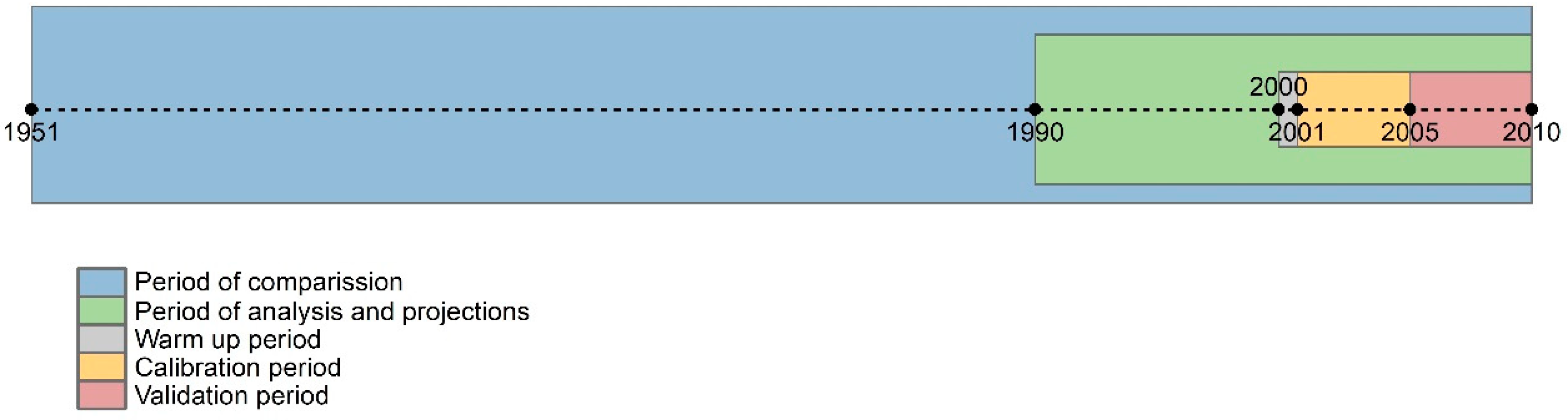
To allow a better understanding of the methodology, Figure 3 details the periods in which each process was carried out. Satisfactory results have been obtained using a 5-year or smaller time window for calibration [55]. Harlin [63] recommends using a calibration period between 2 and 6 years to find optimal parameters for the HBV model, and Brigode et al. [64] indicated that calibration periods longer than 3 years do not necessarily lead to more robust parameter sets. In this study, periods of 1, 5, and 5 years were used for model warm-up, calibration, and validation, respectively (grey, yellow, and red periods in Figure 3).
According to Seibert and Vis [65], one year is sufficient to warm up the model. Therefore, in the calibration and validation processes, the first year of analysis (2000 and 2006, respectively) was discarded to eliminate the influence of the starting values on the results.
3.2.1. Regional Sensitivity Analysis
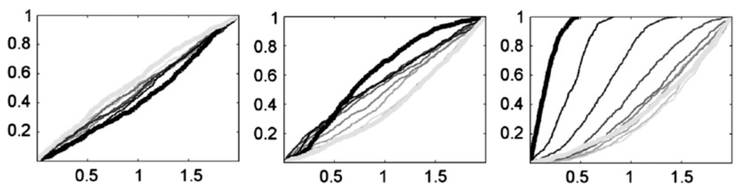
The RSA method consists of generating a sample of N points (simulations) in the feasible space of each parameter, obtained from a previously defined distribution (generally uniform). The parameter sets are ranked from best to worst in terms of the chosen objective function. The ranked population is then divided into ten bins of equal size according to their objective values. The objective values associated with each parameter set are then converted to likelihood measures. The cumulative distribution of each group is then plotted, and the highest likelihood parameter distributions are indicated by bold black lines and the lowest likelihood distributions indicated by light gray lines (see Figure 4 as an example). In order to obtain the best representation of all the parameter sets (models), the calibrated parameters values were obtained according to the 50th percentile in the highest likelihood parameter distributions (bold black lines). Parameter sensitivity can be evaluated by assessing the separation of the ten curves. The greater the separation between curves, the greater the sensitivity of the model to the parameter under analysis. By contrast, the less separated the curves, the less sensitivity of the model to the parameter [54].
In order to independently represent the minimum and maximum mean daily flow trends, two calibrations were carried out based on the root mean square error (RMSE) and transformed root Mean square error (TRMSE) objective functions, which are focused on high and low flows, respectively [66,67]. Additionally, NSE values were calculated for both calibration and validation with the purpose of complementing the overall model performance evaluation (not only focusing on either maximum or minimum flows). The objective functions are described in the following sections (Section 3.2.2, Section 3.2.3 and Section 3.2.4). To validate the models, values within the limit of acceptability for the validation period were sought.
3.2.2. Root Mean Square Error (RMSE)
RMSE can be considered a multi-purpose criterion centered on the simulated hydrograph. This function is focused on high streamflow errors [66,67] and is calculated with Equation (1):
where are the simulated and observed stream flows in time step , respectively, and T is the length of the time series. Because RMSE measures differences between simulated and observed stream flows, it has the unit of measurement of the analyzed data (m3/s). An RMSE equal to zero indicates a perfect fit between the simulated and observed series, while the greater the RMSE value, the worse the fit between simulated and observed data. According to Singh et al. [68], RMSE values less than half of the standard deviation of the observed data can be considered low and indicate good model prediction.
3.2.3. Transformed Root Mean Square Error (TRMSE)
This function emphasizes low flow errors using the Box–Cox transformed [60] root mean square error, as shown in Equations (2) and (3):
where and are the Box–Cox transformed simulated and observed streamflow at time step t, respectively, T is the length of the time series, and has a similar effect as a log transformation [60]. As the RMSE, we deemed less than half of the standard deviation of the transformed observed data to be the value that indicates good model prediction.
3.2.4. Nash–Sutcliffe Efficiency (NSE)
This index determines the relative magnitude of residual variance in comparison to the variance of the measured data [69]. The NSE is obtained with Equation (4):
where are the simulated stream flows in time step , observed stream flows in time step and the average of the observed stream flows, respectively. Meanwhile, T is the length of the time series. NSE values vary between 1 and −∞, with 1 being the optimum value. Normally the value for a model to be considered suitable is NSE = 0.6 [55,70].
3.3. Trend Calculation and Analysis
After the calibration and validation processes, all daily stream flows were simulated, and the annual minimum and maximum values in the 1990–2010 period were extracted for simulations. To assess the effect of the length of the data series on the estimation of trends in the annual maximum and minimum stream flows, three situations were studied by eliminating 2, 5, and 10 years of simulated stream flows. All the possible trends according to the possible combinations (green period in Figure 3) were estimated. This methodology was adopted because information at basin scale in Chile generally does not consist of more than 30 years of records and may even consist of less than 10 years of data. In addition, since performing the entire procedure of randomly eliminating from 1 up to 19 years would significantly increase the computational resources needed, a simpler (reduced) approach was used, removing 2, 5, and 10 years from the analyses. Thus, totals of 210 (2 years removed), 20,349 (5 years removed), and 352,716 (10 years removed) possible combinations were analyzed. Then the trends of all the resulting time series (combinations) were calculated by the least squares method (green period in Figure 3). This is the most popular method used to determine the position of the trend line of a given time series. The trend line is technically called the best fit. In this method, a mathematical relationship is established between the time factor and the variable given [71]. The equation of the trend line can be expressed as
where represents the trend of the variable when and represents the slope of the trend line. If is positive, the trend line will be upward, and if is negative the trend line will be downward.
To analyze the influence of the length of each data set, the generalized likelihood uncertainty estimation (GLUE) method [72] was applied to the resultant estimated trends. Unlike the GLUE method, in which uncertainty bands are derived from the outputs that only produce adequate results based on a performance measure, in this study the median and the uncertainty bands between 5% and 95% of all the calculated trends were calculated. Finally, the results of each situation were compared with the long-term trend derived from observed streamflow data of the maximum and minimum flows over the entire period of records from the Río Allipén en Los Laureles station (1951–2010; blue period in Figure 3).
4. Results
4.1. Model Calibration and Validation
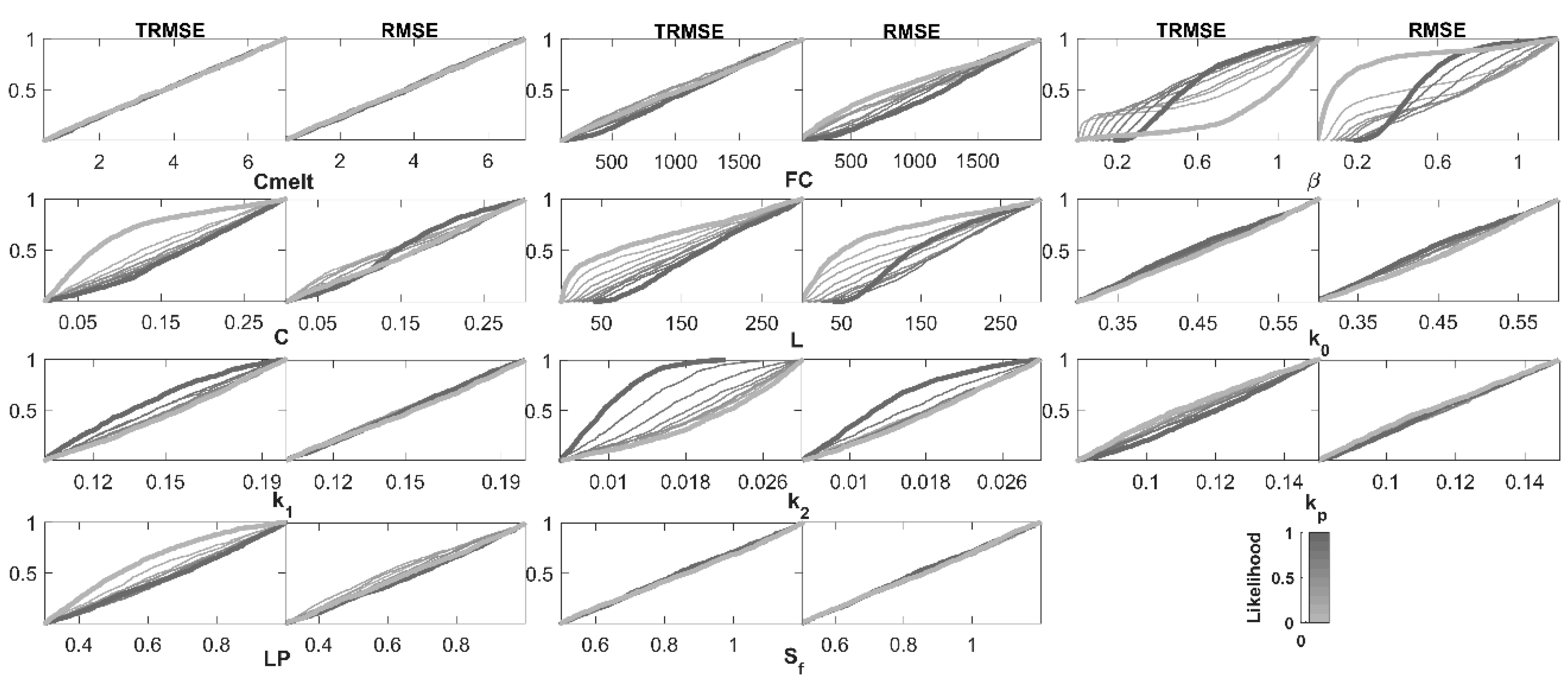
Figure 5 presents the results of the RSA in the calibration process focused on high and low flows (TRMSE and RMSE, respectively). In both cases, high sensitivity of the results to variations in parameters β and L is observed. β represents the contribution of precipitation and snowmelt to soil storage and runoff, and L is the limit for the quick response. Most stream flows in the watershed are of a pluvial origin; therefore, the model does not present sensitivity to parameters associated with the snow accumulation and snowmelt processes (module) (Cmelt and Sf).
Along with the model sensitivity to β and L, in the calibration based on RMSE, it is observed that the parameter that most influences the model performance is FC, which represents field capacity. In addition, the results based on TRMSE indicate that the model is sensitive to K2 (slow-response recession coefficient). The highest stream flows are a result of high precipitation in winter periods, when soil storage can approach its capacity; therefore, the process that takes on the greatest importance during high stream flows is soil moisture (FC). Meanwhile, in the recession and stable-streamflow periods (spring-summer), groundwater runoff and the low snowmelt input are represented in the model by the increase in sensitivity to the slow response (K2).
Table 2 shows the values of the objective functions calculated for the calibration and validation, while Table 3 shows the parameter sets obtained in each ease. The reference values of the objective functions are indicated in parentheses. For the RMSE and TRMSE values, Parra et al. [55], Singh et al. [58], and Moriasi et al. [60] suggest that the results must be less than half of the standard deviation of the observed and transformed data, respectively, and the NSE values must be greater than 0.6. According to the calculated indices, the parameter sets in both cases are suitable for simulating the stream flows of the Allipén River watershed.
In Table 3, it is observed that L is greater for low stream flows than for high stream flows and k2 is lower for low stream flows than for high stream flows, which shows that the model calibrated with TRMSE emphasizes streamflow stability through the contribution of groundwater (slow process) to the total streamflow, and the model calibrated with RMSE is focused on quick responses (peaks) through the contribution of surface runoff to the total streamflow.
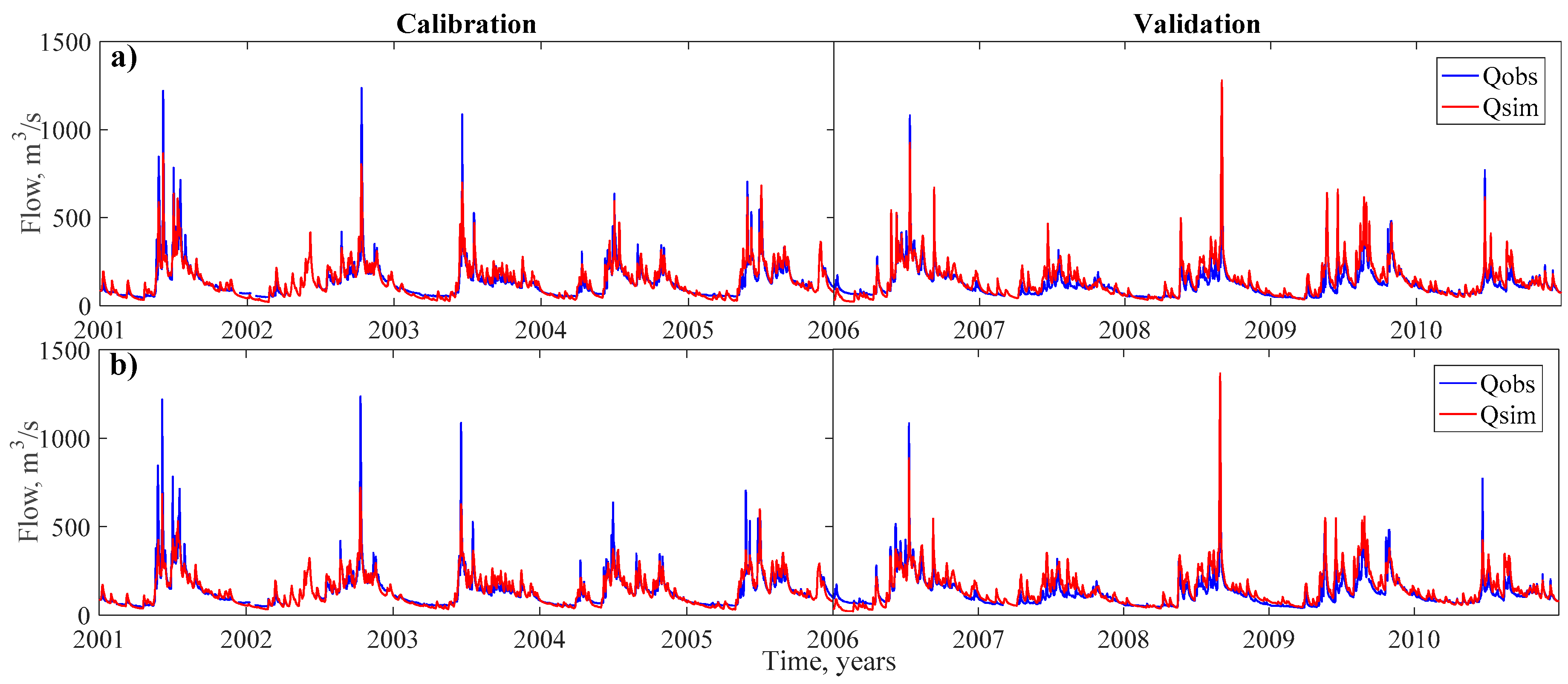
According to the sensitivity analysis, the objective functions, and the obtained parameter sets, the model is deemed suitable for use in the subsequent analyses. Figure 6 shows a comparison of the observed and simulated stream flows in the calibration and validation processes for each case.
4.2. Trend Uncertainty Analysis
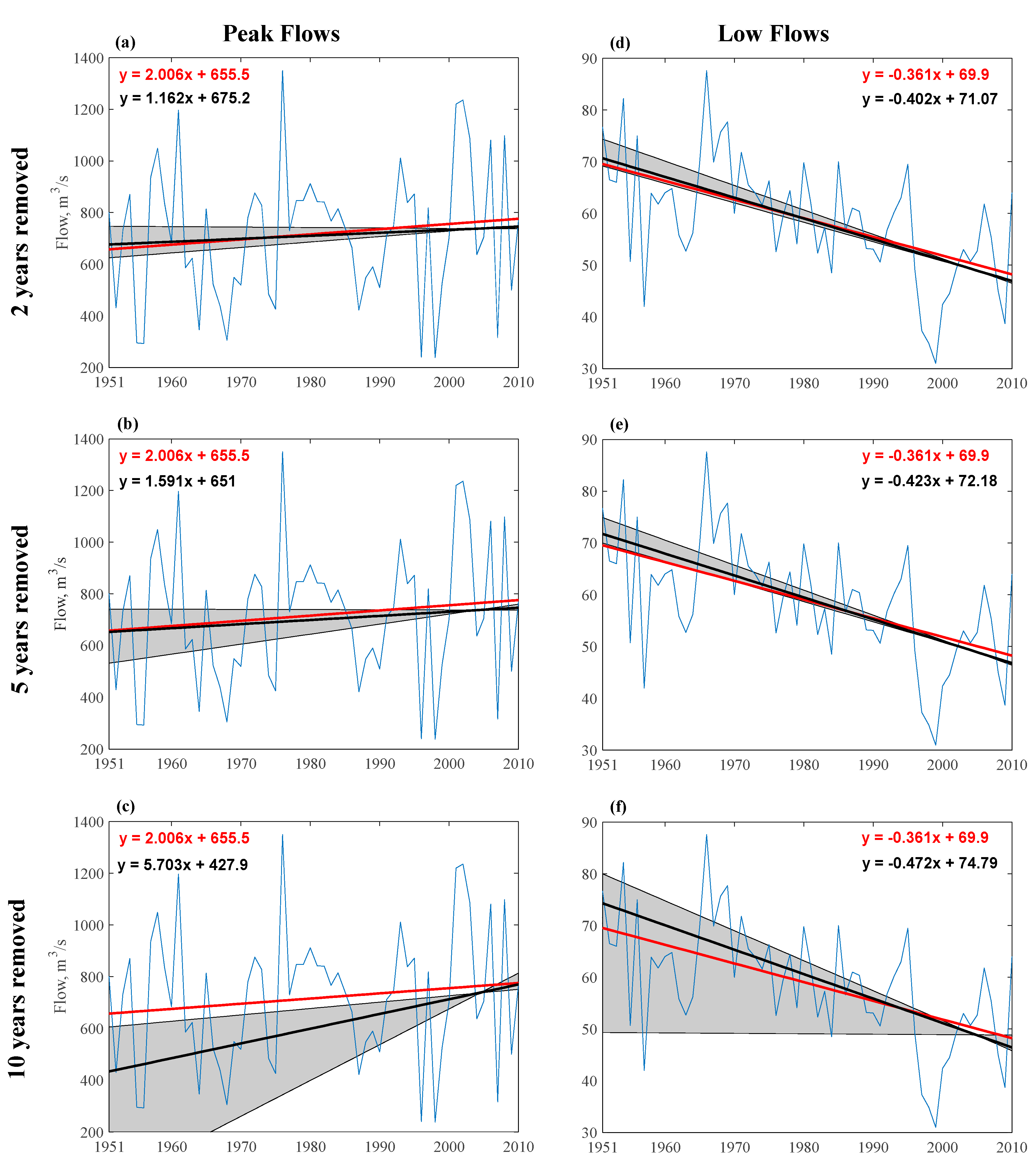
Figure 7a–c shows the maximum daily streamflow trends, the median of the trends obtained by eliminating 2, 5, and 10 years of information, and the uncertainty bands for each case. The same is shown in Figure 7d–f for the annual minimum daily stream flows. It is observed that extreme events tend to increase in magnitude, as the maximum streamflow trend is positive, and the minimum streamflow trend is negative.
In Figure 7a,b,d,e it is observed that the medians of the trends are similar to the observed streamflow trend. Trends of the annual minimum daily stream flows present greater uncertainty than those of the annual maximum daily stream flows. As the uncertainty of trends calculated using 16 and 19 years is similar to that of the trend estimated from data, it proves suitable to use either 16 or 19 years of simulated flows to estimate the basin annual maximum and minimum flow trends. Meanwhile, for the trends estimated with 11 years of simulated data, uncertainty increases, and the slope of the median differs from the trend obtained from the streamflow records available in the watershed.
In south-central Chile, a decreasing precipitation and increasing temperature trend has been recorded [24,25,26,30]. Higher temperatures may lead to earlier snowmelt and to a shift of high flows from spring to winter. Earlier recession flows will be therefore expected with lower flows in summer, explaining the negative trend of the low flows observed in Figure 7.
5. Conclusions
The lack of stream flow records is one of the most common drawbacks when conducting hydrological analyses. Results of the estimation of annual minimum and maximum flow trends using hydrological modeling in watersheds with limited hydrological (meteorological and streamflow) information were presented in the present study. To estimate these trends, a 21-year period of observed and simulated stream flows was used. To account for data scarcity, trends were estimated in three situations (by eliminating 2, 5, and 10 years of simulated stream flows) and accounting for the possible combinations of the gaps.
According to the results of the trend analysis, minimum extreme flows tend to decrease, while maximum extremes tend to increase. The Allipén River presents a mixed hydrological regime where higher temperatures increase the snow melt, contributing to the increasing trend of high flows. Additionally, to derive the long-term trends of annual peak and low flows it is necessary to simulate at least 16 years of flows; otherwise, the resulting uncertainty is high, with levels at which even opposing extreme flow trends are obtained.
This study presented an approach to estimate flow trends in basins with limited stream-flow information. A minimum recommendable amount of data (16 year of data) is given in order to obtain results under controlled uncertainty. The presented method is not limited to the use of other hydrological models, objective functions, and/or sensitivity analysis. Despite the results presented here, more robust analyses can be obtained if basins with different characteristics and more extensive gaps of data are analyzed. Future research might complement the current research by including regional analyses and different trend estimation methods (e.g., parametric vs. nonparametric).
Author Contributions
Conceptualization, Y.M. and E.M.; Methodology, Y.M. and E.M.; Software, Y.M.; Formal Analysis, Y.M.; Investigation, Y.M.; Data Curation, Y.M.; Writing—Original Draft Preparation, Y.M. and E.M.; Visualization, Y.M. and E.M.; Supervision, E.M. All authors have read and agreed to the published version of the manuscript.
Funding
Dirección de Investigación, Universidad Católica de la Santísima Concepción, DINREG 03/2019.
Acknowledgments
The authors thank the Dirección General de Aguas (National Water Directorate) for providing the data for the development of this study and the Civil Engineering PhD program of the Universidad Católica de la Santísima Concepción for contributing to this research.
Conflicts of Interest
The authors declare no conflict of interest.
References
- Muñoz, E. Perfeccionamiento de un Modelo Hidrológico Aplicación de Análisis de Identificabilidad Dinámico y uso de Datos Grillados. Ph.D. Thesis, Departamento de Recursos Hídricos, Universidad de Concepción, Chillán, Chile, 2011. [Google Scholar]
- Buendia, C.; Batalla, R.J.; Sabater, S.; Palau, A.; Marcé, R. Runoff trends driven by climate and afforestation in a Pyrenean Basin. Land Degrad. Dev. 2016, 27, 823–838. [Google Scholar] [CrossRef] [Green Version]
- Sharma, P.J.; Patel, P.L.; Jothiprakash, V. Impact of rainfall variability and anthropogenic activities on streamflow changes and water stress conditions across Tapi Basin in India. Sci. Total Environ. 2019, 687, 885–897. [Google Scholar] [CrossRef] [PubMed]
- Cheng, Q.; Li, L.; Wang, L. Characterization of peak flow events with local singularity method. Nonlinear Process. Geophys. 2009, 16, 503–513. [Google Scholar] [CrossRef]
- Diop, D.; Yaseen, Z.M.; Bodian, A.; Djaman, K.; Brown, L. Trend analysis of streamflow with different time scales: A case study of the upper Senegal River. ISH J. Hydraul. Eng. 2018, 24, 105–114. [Google Scholar] [CrossRef]
- Philip, L.; Kumar, L.; Koech, R. Temporal Variability and Trends of Rainfall and Streamflow in Tana River Basin, Kenya. Sustainability 2017, 9, 1963. [Google Scholar] [CrossRef] [Green Version]
- Huang, X.; Zhao, J.; Li, W.; Jiang, H. Impact of climatic change on streamflow in the upper reaches of the Minjiang River, China. Hydrol. Sci. J. 2014, 59, 154–164. [Google Scholar] [CrossRef]
- Salmoral, G.; Willaarts, B.A.; Troch, P.A.; Garrido, A. Drivers influencing streamflow changes in the Upper Turia basin, Spain. Sci. Total Environ. 2015, 503, 258–268. [Google Scholar] [CrossRef]
- Shah, H.L.; Mishra, V. Hydrologic changes in Indian subcontinental river basins (1901–2012). J. Hydrometeorol. 2016, 17, 2667–2687. [Google Scholar] [CrossRef]
- Li, B.; Li, C.; Liu, J.; Zhang, Q.; Duan, L. Decreased streamflow in the Yellow River basin, China: Climate change or human-induced? Water. 2017, 9, 116. [Google Scholar] [CrossRef]
- Ghaleni, M.M.; Ebrahimi, K. Effects of human activities and climate variability on water resources in the Saveh plain, Iran. Environ. Monit. Assess. 2015, 187, 35. [Google Scholar] [CrossRef]
- Suttles, K.M.; Singh, N.K.; Vose, J.M.; Martin, K.L.; Emanuel, R.E.; Coulston, J.W.; Saia, S.M.; Crump, M.T. Assessment of hydrologic vulnerability to urbanization and climate change in a rapidly changing watershed in the Southeast US. Sci. Total Environ. 2018, 645, 806–816. [Google Scholar] [CrossRef] [PubMed]
- Somorowska, U.; Łaszewski, M. Quantifying streamflow response to climate variability, wastewater inflow, and sprawling urbanization in a heavily modified river basin. Sci. Total Environ. 2019, 656, 458–467. [Google Scholar] [CrossRef] [PubMed]
- Da Silva, R.M.; Santos, C.A.; Moreira, M.; Corte-Real, J.; Silva, V.C.; Medeiros, I.C. Rainfall and river flow trends using Mann–Kendall and Sen’s slope estimator statistical tests in the Cobres River basin. Nat. Hazards 2015, 77, 1205–1221. [Google Scholar] [CrossRef]
- Samaniego, L.; Bardossy, A.; Kumar, R. Streamflow prediction in ungauged catchments using copula-based dissimilarity measures. Water Resour. Res. 2010, 46, W02506. [Google Scholar] [CrossRef]
- Betterle, A.; Schirmer, M.; Botter, G. Flow dynamics at the continental scale: Streamflow correlation and hydrological similarity. Hydrol. Process. 2019, 33, 627–646. [Google Scholar] [CrossRef] [Green Version]
- Wang, Y.C.; Chen, S.T.; Yu, P.S.; Yang, T.C. Storm-even rainfall–runoff modelling approach for ungauged sites in Taiwan. Hydrol. Process. 2008, 22, 4322–4330. [Google Scholar] [CrossRef]
- Besaw, L.E.; Rizzo, D.M.; Bierman, P.R.; Hackett, W.R. Advances in ungauged streamflow prediction using artificial neural networks. J. Hydrol. 2010, 386, 27–37. [Google Scholar] [CrossRef]
- Gayathri, K.D.; Ganasri, B.P.; Dwarakish, G.S. A review on hydrological models. Aquat. Procedia 2015, 4, 1001–1007. [Google Scholar] [CrossRef]
- Wagener, T.; Boyle, D.; Lees, M.; Wheater, H.; Gupta, H.; Sorooshian, S. A framework for development and application of hydrological models. Hydrol. Earth Syst. Sci. 2001, 5, 13–26. [Google Scholar] [CrossRef]
- Wagener, T.; Wheater, H.S.; Gupta, H.V. Identification and evaluation of watershed models. Calibration Watershed Models 2003, 29–47. [Google Scholar] [CrossRef] [Green Version]
- Wakigari, S. Evaluation of conceptual hydrological models in data scarce region of the Upper Blue Nile Basin: Case of the Upper Guder catchment. Hydrology 2017, 4, 59. [Google Scholar] [CrossRef] [Green Version]
- Demaria, E.M.C.; Maurer, E.P.; Thrasher, B.; Vicuña, S.; Meza, F.J. Climate change impacts on an alpine watershed in Chile: Do new model projections change the story? J. Hydrol. 2013, 502, 128–138. [Google Scholar] [CrossRef]
- Boisier, J.P.; Rondanelli, R.; Garreaud, R.; Muñoz, F. Anthropogenic and natural contributions to the Southeast Pacific precipitation decline and recent megadrought in central Chile. Geophys. Res. Lett. 2016, 43, 413–421. [Google Scholar] [CrossRef] [Green Version]
- Garreaud, R.D.; Alvarez-Garreton, C.; Barichivich, J.; Boisier, J.P.; Duncan, C.; Galleguillos, M.; Zambrano-Bigiarini, M. The 2010–2015 megadrought in central Chile: Impacts on regional hydroclimate and vegetation. Hydrol. Earth Syst. Sci. 2017, 21, 6307–6327. [Google Scholar] [CrossRef] [Green Version]
- Sarricolea, P.; Meseguer-Ruiz, Ó.; Serrano-Notivoli, R.; Soto, M.V.; Martin-Vide, J. Trends of daily precipitation concentration in Central-Southern Chile. Atmos. Res. 2018, 215, 85–98. [Google Scholar] [CrossRef]
- Mernild, S.H.; Liston, G.E.; Hiemstra, C.A.; Malmros, J.K.; Yde, J.C.; McPhee, J. The Andes Cordillera. Part I: Snow distribution, properties, and trends (1979-2014). Int. J. Climatol. 2016, 37, 1680–1698. [Google Scholar] [CrossRef]
- Pérez, T.; Mattar, C.; Fuster, R. Decrease in Snow Cover over the Aysén River Catchment in Patagonia, Chile. Water 2018, 10, 619. [Google Scholar] [CrossRef] [Green Version]
- Ruiz Pereira, S.F.; Veettil, B.K. Glacier decline in the Central Andes (33° S): Context and magnitude from satellite and historical data. J. S. Am. Earth Sci. 2019, 94, 102249. [Google Scholar] [CrossRef]
- Burger, F.; Brock, B.; Montecinos, A. Seasonal and elevational contrasts in temperature trends in Central Chile between 1979 and 2015. Glob. Planet. Chang. 2018, 162, 136–147. [Google Scholar] [CrossRef]
- Meseguer-Ruiz, O.; Ponce-Philimon, P.I.; Quispe-Jofré, A.S.; Guijarro, J.A.; Sarricolea, P. Spatial behaviour of daily observed extreme temperatures in Northern Chile (1966–2015): Data quality, warming trends, and its orographic and latitudinal effects. Stoch. Environ. Res. Risk A. 2018, 32, 3503–3523. [Google Scholar] [CrossRef] [Green Version]
- Alvarez-Garreton, C.; Mendoza, P.A.; Boisier, J.P.; Addor, N.; Galleguillos, M.; Zambrano-Bigiarini, M.; Lara, A.; Puelma, C.; Cortes, G.; Garreaud, R.; et al. The CAMELS-CL dataset: Catchment attributes and meteorology for large sample studies–Chile dataset. Hydrol. Earth Syst. Sci. 2018, 22, 5817–5846. [Google Scholar] [CrossRef] [Green Version]
- Muñoz, E.; Acuña, M.; Lucero, J.; Rojas, I. Correction of Precipitation Records through Inverse Modeling in Watersheds of South-Central Chile. Water 2018, 10, 1092. [Google Scholar] [CrossRef] [Green Version]
- Rubio-Álvarez, E.; McPhee, J. Patterns of spatial and temporal variability in streamflow records in south central Chile in the period 1952–2003. Water Resour. Res. 2010, 46, W05514. [Google Scholar] [CrossRef]
- Muñoz, A.A.; González-Reyes, A.; Lara, A.; Sauchyn, D.; Christie, D.; Puchi, P.; Urrutia-Jalabert, R.; Toledo-Guerrero, I.; Aguilera-BettiIgnacio, I.; Mundo, I.; et al. Streamflow variability in the Chilean Temperate-Mediterranean climate transition (35° S–42° S) during the last 400 years inferred from tree-ring records. Clim. Dyn. 2016, 47, 4051–4066. [Google Scholar] [CrossRef]
- Lara, A.; Bahamondez, A.; González-Reyes, A.; Muñoz, A.A.; Cuq, E.; Ruiz-Gómez, C. Reconstructing streamflow variation of the Baker River from tree-rings in Northern Patagonia since 1765. J. Hydrol. 2015, 529, 511–523. [Google Scholar] [CrossRef]
- Barria, P.; Peel, M.C.; Walsh, K.J.E.; Muñoz, A. The first 300-year streamflow reconstruction of a high-elevation river in Chile using tree rings. Int. J. Climatol. 2017, 38, 436–451. [Google Scholar] [CrossRef]
- Anderson, S.; Ogle, R.; Tootle, G.; Oubeidillah, A. Tree-Ring Reconstructions of Streamflow for the Tennessee Valley. Hydrology 2019, 6, 34. [Google Scholar] [CrossRef] [Green Version]
- Chen, F.; Shang, H.; Panyushkina, I.P.; Meko, D.M.; Yu, S.; Yuan, Y.; Chen, F. Tree-ring reconstruction of Lhasa River streamflow reveals 472 years of hydrologic change on southern Tibetan Plateau. J. Hydrol. 2019, 572, 169–178. [Google Scholar] [CrossRef]
- Liu, N.; Bao, G.; Liu, Y.; Linderholm, H.W. Two Centuries-Long Streamflow Reconstruction Inferred from Tree Rings for the Middle Reaches of the Weihe River in Central China. Forests 2019, 10, 208. [Google Scholar] [CrossRef] [Green Version]
- Strange, B.M.; Maxwell, J.T.; Robeson, S.M.; Harley, G.L.; Therrell, M.D.; Ficklin, D.L. Comparing Three Approaches to Reconstructing Streamflow Using Tree Rings in the Wabash River Basin in the Midwestern, US. J. Hydrol. 2019, 573, 829–840. [Google Scholar] [CrossRef]
- Cunderlik, J.M.; Burn, D.H. Local and Regional Trends in Monthly Maximum Flows in Southern British Columbia. Can. Water Resour. J. 2002, 27, 191–212. [Google Scholar] [CrossRef] [Green Version]
- Kundzewicz, Z.W.; Graczyk, D.; Maurer, T.; Pińskwar, I.; Radziejewski, M.; Svensson, C.; Szwed, M. Trend detection in river flow series: 1. Annual maximum flow. Hydrol. Sci. J. 2005, 50, 810. [Google Scholar] [CrossRef]
- Burn, D.H.; Sharif, M.; Zhang, K. Detection of trends in hydrological extremes for Canadian watersheds. Hydrol. Process. 2010, 24, 1781–1790. [Google Scholar] [CrossRef]
- Bormann, H.; Pinter, N. Trends in low flows of German rivers since 1950: Comparability of different low-flow indicators and their spatial patterns. River Res. Appl. 2017, 33, 1191–1204. [Google Scholar] [CrossRef]
- Dirección General de Aguas. Diagnóstico y Clasificación de los Cursos y Cuerpos de Agua Según Objetivos de Calidad; Cuenca del Río Toltén; Ministerio de Obras Públicas: Santiago, Chile, 2004.
- Sheffield, J.; Goteti, G.; Wood, E. Development of a 50-year high-resolution global dataset of meteorological forcings for land surface modelling. J. Clim. 2006, 19, 3088–3111. [Google Scholar] [CrossRef] [Green Version]
- Thornthwaite, C. An Approach toward a Rational Classification of Climate. Geogr. Rev. 1948, 38, 55–94. [Google Scholar] [CrossRef]
- Bergström, S. Utvechling och Tillämpning av en Digital Avrinningsmodell (Development and Application of a Digital Runoff Model; Notiser och Preliminära Rapporter. Serie HydrologI. 22; Swedish Meteorological and Hydrological Institute (SMHI): Norrköping, Sweden, 1972. (In Swedish) [Google Scholar]
- Driessen, T.; Hurkmans, R.; Terink, W.; Hazenberg, P.; Torfs, P.; Uijlenhoet, R. The hydrological response of the Ourthe catchment to climate change as modelled by the HBV model. Hydrol. Earth Syst. Sci. 2010, 14, 651–665. [Google Scholar] [CrossRef] [Green Version]
- Saibert, J. Multi-criteria calibration of a conceptual runoff model using a genetic algorithm. Hydrol. Earth Syst. Sci. 2000, 4, 215–224. [Google Scholar] [CrossRef] [Green Version]
- Lindström, G.; Johansson, B.; Persson, M.; Gardelin, M.; Bergström, S. Development and test of the distributed HBV-96 hydrological model. J. Hydrol. 1997, 201, 272–288. [Google Scholar] [CrossRef]
- Rusli, S.; Yudianto, D.; Liu, J. Effects of temporal variability on HBV model calibration. Water Sci. Eng. 2015, 8, 291–300. [Google Scholar] [CrossRef] [Green Version]
- Wagener, T.; Kollat, J. Numerical and visual evaluation of hydrological and environmental models using the Monte Carlo analysis toolbox. Environ. Model. Softw. 2007, 22, 1021–1033. [Google Scholar] [CrossRef]
- Parra, V.; Fuentes-Aguilera, P.; Muñoz, E. Identifying advantages and drawbacks of two hydrological models based on a sensitivity analysis: a study in two Chilean watersheds. Hydrolog. Sci. J. 2018, 63, 1831–1843. [Google Scholar] [CrossRef]
- Aghakouchak, A.; Habib, E. Application of a Conceptual Hydrologic Model in Teaching Hydrologic Processes. Int. J. Eng. Educ. 2010, 26, 963–973. [Google Scholar]
- Bergström, S. The HBV model–Its structure and applications; Swedish Meteorological and Hydrological Institute (SMHI): Norrköping, Sweden, 1992; Volume 4, ISSN 0283-1104. [Google Scholar]
- Saibert, J. HBV-light Version 2 User’s Manual; Department of Physical Geography, Stockholm University: Stockholm, Sweden, 2005. [Google Scholar]
- Muñoz, E.; Rivera, D.; Vergara, F.; Tume, P.; Arumí, J. Identifiability analysis: towards constrained equifinality and reduced uncertainty in a conceptual model. Hydrol. Sci. J. 2014, 59, 1690–1703. [Google Scholar] [CrossRef]
- Kollat, J.B.; Reed, P.M.; Wagener, T. When are multiobjective calibration trade-offs in hydrologic models meaningful? Water Resour. Res. 2012, 48, W3520. [Google Scholar] [CrossRef]
- Spear, R.; Hornberger, G. Eutrophication in Peel Inlet, II, identification of critical uncertainties via generalised sensitivity analysis. Water Resour. Res. 1980, 14, 43–49. [Google Scholar] [CrossRef]
- Sarrazin, F.; Pianosi, F.; Wagener, T. Global sensitivity analysis of environmental models: Convergence and validation. Environ. Model. Softw. 2016, 79, 135–152. [Google Scholar] [CrossRef] [Green Version]
- Harlin, J. Development of a process oriented calibration scheme for the HBV hydrological model. Nord. Hydrol. 1991, 22, 15–36. [Google Scholar] [CrossRef]
- Brigode, P.; Oudin, L.; Perrin, C. Hydrological model parameter instability: A source of additional uncertainty in estimating the hydrological impacts of climate change? J. Hydrol. 2013, 476, 410–425. [Google Scholar] [CrossRef] [Green Version]
- Seibert, J.; Vis, M. Teaching hydrological modeling with a user-friendly catchment-runoff-model software package. Hydrol. Earth Syst. Sci. 2012, 16, 3315–3325. [Google Scholar] [CrossRef] [Green Version]
- Wagener, T.; van Werkhoven, K.; Reed, P.; Tang, Y. Multiobjective sensitivity analysis to understand the information content in streamflow observations for distributed watershed modeling. Water Resour. Res. 2009, 45, W02501. [Google Scholar] [CrossRef] [Green Version]
- Pfannerstill, M.; Guse, B.; Fohrer, N. Smart low flow signature metrics for an improved overall performance evaluation of hydrological models. J. Hydrol. 2014, 510, 447–458. [Google Scholar] [CrossRef]
- Singh, J.; Knapp, H.V.; Demissie, M. Hydrologic Modeling of the Iroquois River Watershed using HSPF and SWAT ISWS CR 2004-08; Illinois State Water Survey: Champaign, IL, USA, 2004; Available online: http://hdl.handle.net/2142/94220 (accessed on 20 July 2019).
- Nash, J.E.; Sutcliffe, J.V. River Flow Forecasting Through Conceptual Models, Part I, A Discussion of Principles. J. Hydrol. 1970, 10, 282–290. [Google Scholar] [CrossRef]
- Moriasi, D.N.; Arnold, J.G.; Van Liew, M.W.; Bingner, R.L.; Harmel, R.D.; Veith, T.L. Model evaluation guidelines for systematic quantification of accuracy in watershed simulations. Trans. ASABE 2007, 50, 885–900. [Google Scholar] [CrossRef]
- Molugaram, K.; Rao, G.S. Chapter 12-Analysis of Time Series. In Statistical Techniques for Transportation Engineering; Molugaram, K., Rao, G.S., Shah, A., Davergave, N., Eds.; Butterworth-Heinemann: Oxford, UK, 2017; pp. 451–462. [Google Scholar]
- Beven, K.; Binley, A. The future of distributed models: Model calibration and uncertainty prediction. Hydrol. Process. 1992, 6, 279–298. [Google Scholar] [CrossRef]
Figure 1.
Geographic location and digital elevation model of the Allipén River watershed at the Río Allipén en Los Laureles station. The light blue dot shows the location of the streamflow monitoring station, the dark blue dots the locations of the rain gauge stations, and the red dots the gridded temperature stations published by Princeton University.

Figure 2.
Conceptual diagram of the Hydrologiska Byråns Vattenbalansavdelning (HBV) model.

Figure 3.
Timeline of the periods in which each process was carried out. Warm-up period (2000), calibration period (2001–2005), validation period (2006–2010), analysis and trend projection period (1990–2010), and complete streamflow records for comparison (1951–2010).
Figure 3.
Timeline of the periods in which each process was carried out. Warm-up period (2000), calibration period (2001–2005), validation period (2006–2010), analysis and trend projection period (1990–2010), and complete streamflow records for comparison (1951–2010).

Figure 4.
Regional sensitivity analysis plots example obtained from Wagener and Kollat [54].
Figure 4.
Regional sensitivity analysis plots example obtained from Wagener and Kollat [54].

Figure 5.
Regional sensitivity analysis plots example.

Figure 6.
Observed and simulated flows in the calibration and validation based on the (a) RMSE (b) TRMSE objective functions.
Figure 6.
Observed and simulated flows in the calibration and validation based on the (a) RMSE (b) TRMSE objective functions.

Figure 7.
Uncertainty bands (gray areas), median of the simulated trends (black lines), observed trends (red lines) of maximum (top) and annual minimum mean daily flows (bottom), and trend equations. For (a) and (d) a simulation of 19 years, (b) and (e) a simulation of 16 years, and (c) and (f) a simulation of 11 years. In addition, the observed annual maximum (top) and minimum extreme flow series (bottom) are shown in the background (blue line).


Table 1.
Model parameters and initial ranges used for the analysis.
| Parameter | Description | Range |
|---|---|---|
| Mass balance | ||
| A | Precipitation modification parameter | 0.8–2.5 |
| Snow module | ||
| TT (°C) | Threshold temperature that indicates the initiation of snowmelt (normally 0 °C) | 0 |
| Cmelt | Fraction of snow that melts above the threshold temperature (TT) from the beginning of snowmelt. | 0.5–7 |
| Snow accumulation adjustment factor | 0.5–1.2 | |
| Moisture module | ||
| FC (mm) | Field capacity (storage in the soil layer) | 0–2000 |
| Empirical coefficient that represents the soil moisture variation in the area | 0–7 | |
| LP | Fraction of field capacity to calculate the permanent wilting point (PWP = LP*FC) | 0.3–1 |
| C () | Correction factor for potential evapotranspiration | 0.01–0.3 |
| Response module | ||
| L (mm) | Threshold for quick runoff response | 0–100 |
| () | Quick response coefficient (upper reservoir) | 0.3–0.6 |
| () | Slow response coefficient (upper reservoir) | 0.1–0.2 |
| () | Lower reservoir response coefficient | 0.01–0.1 |
| () | Maximum flow coefficient for percolation | 0.01–0.1 |
Table 2.
Objective function values and the reference performance rating in parenthesis.
| Process | Period | Peak Flows | Low Flows | ||
|---|---|---|---|---|---|
| RMSE | NSE | TRMSE | NSE | ||
| Calibration | 2001–2005 | 45.1 (<54.8) | 0.81 (>0.6) | 0.89 (<2.0) | 0.77 (>0.6) |
| Validation | 2007–2010 | 39.4 (<40.1) | 0.73 (>0.6) | 0,91 (<1.1) | 0.84 (>0.6) |
Table 3.
Parameter values obtained after calibration and validation focused on high and low flows (separately).
Table 3.
Parameter values obtained after calibration and validation focused on high and low flows (separately).
| Parameter | Peak Flows | Low Flows |
|---|---|---|
| A | 1.2 | 1.2 |
| TT (°C) | 0 | 0 |
| 4.01 | 3.65 | |
| FC (mm) | 1280 | 1030 |
| 0.15 | 0.18 | |
| 0.50 | 0.60 | |
| L (mm) | 115 | 180 |
| 0.44 | 0.44 | |
| 0.15 | 0.14 | |
| 0.015 | 0.008 | |
| 0.11 | 0.12 | |
| LP | 0.68 | 0.68 |
| 0.83 | 0.85 |
© 2020 by the authors. Licensee MDPI, Basel, Switzerland. This article is an open access article distributed under the terms and conditions of the Creative Commons Attribution (CC BY) license (http://creativecommons.org/licenses/by/4.0/).
Share and Cite
MDPI and ACS Style
Medina, Y.; Muñoz, E. Estimation of Annual Maximum and Minimum Flow Trends in a Data-Scarce Basin. Case Study of the Allipén River Watershed, Chile. Water 2020, 12, 162. https://doi.org/10.3390/w12010162
AMA Style
Medina Y, Muñoz E. Estimation of Annual Maximum and Minimum Flow Trends in a Data-Scarce Basin. Case Study of the Allipén River Watershed, Chile. Water. 2020; 12(1):162. https://doi.org/10.3390/w12010162
Chicago/Turabian StyleMedina, Yelena, and Enrique Muñoz. 2020. "Estimation of Annual Maximum and Minimum Flow Trends in a Data-Scarce Basin. Case Study of the Allipén River Watershed, Chile" Water 12, no. 1: 162. https://doi.org/10.3390/w12010162
Note that from the first issue of 2016, this journal uses article numbers instead of page numbers. See further details here.