Numerical Simulation of the Fluid–Solid Coupling Mechanism of Internal Erosion in Granular Soil


1
State Key Laboratory of Eco-Hydraulics in Northwest Arid Region of China, Xi’an University of Technology, Xi’an 710048, China
2
School of Civil Engineering, Xijing University, Xi’an 710123, China
*
Author to whom correspondence should be addressed.
Water 2020, 12(1), 137; https://doi.org/10.3390/w12010137
Submission received: 12 November 2019
/
Revised: 27 December 2019
/
Accepted: 27 December 2019
/
Published: 1 January 2020
(This article belongs to the Section Hydraulics and Hydrodynamics)
Abstract
:Internal erosion involves migration and loss of soil particles due to seepage. The process of fluid–solid interaction is a complex multiphase, coupled nonlinear dynamic problem. In this study, we used Particle Flow Code (PFC3D, three-dimensional PFC) software to model solid particles, and we applied computational fluid dynamics (CFD) and the coarse mesh element method to solve the local Navier–Stokes equations. An information-exchange process for the PFC3D and CFD calculations was used to achieve fluid–solid coupling. We developed a numerical model for internal erosion of the soil and conducted relevant experiments to verify the usability of the numerical model. The mechanism of internal erosion was observed by analyzing the evolution of model particle migration, contact force, porosity, particle velocity, and mass-loss measurement. Moreover, we provide some ideas for improving the calculation efficiency of the model. This model can be used to predict the initiation hydraulic gradient and skeleton-deformation hydraulic gradient, which can be used for the design of internal erosion control.
1. Introduction
Internal erosion is the formation of pipes in the soil under seepage conditions. The mechanism of internal erosion can be classified as concentrated leak erosion, backward erosion, contact erosion, and suffusion [1]. When soil particles are gap-graded, fine particles in the soil move and loosen under seepage force, and seepage failure occurs due to suffusion of the soil. In this paper, what we refer to as internal erosion is primarily suffusion. Dikes and unpartitioned homogeneous dams are highly susceptible to internal erosion. Piping is estimated to account for 43% of dam failures. In addition, 54% of the dams built after 1950 failed because of pipe formation [2,3,4].
The internal erosion of the soil is difficult to study and analyze, as it generally occurs underground. Furthermore, it is influenced by many factors, such as particle size gradation [5,6], consolidation degree, porosity, and hydraulic gradient. Internal erosion has always been a major focus area in the study of hydraulics. Scholars have developed various methods for exploring the factors that influence internal erosion. In early studies, Bligh [7] and Lane [8] obtained a series of empirical formulas through statistical analysis of a large number of engineering examples, which provided a direction for internal erosion research. Terzaghi [9] established a mathematical model of piping erosion that analyzes the force balance from the vertical direction, and also established a formula for calculating the critical hydraulic gradient of the soil infiltration failure. With the continuing development in science and technology, research techniques make the course of piping erosion visualization. Rosenbrand [10] used the method of tracing to further explain the mechanism of piping erosion by studying the relationship between the movement of soil particles and the process of piping erosion. Moffat et al. [11] used the method of laboratory testing to record the change of hydraulic gradient and axial displacement of samples and qualitatively explained the spacetime evolution process of the internal instability of the samples. Sibille et al. [12], Hunter [13], and Tomlinson and Vaid [14] used glass beads, broken glass, and other transparent materials, instead of sand, to simulate the occurrence of internal erosion. The researchers investigated the influence of certain factors internal erosion, such as particle size gradation, confining pressure, consolidation degree, filter layer thickness, hydraulic gradient, and gradient growth rate. They observed the dispersion and migration of particles during the erosion process and the formation process of leakage piping.
The methods described above were used to study a series of factors that influence internal erosion, thereby contributing to the fundamental understanding of the mechanism of internal erosion. However, these research methods lack quantitative analysis of fluid–solid interactions and cannot explain the microscopic mechanical behavior of particles. As a result of advancements in computer technology, the numerical simulation research method can now be employed to address this limitation and produce high precision. Some scholars have used the finite element method (FEM) [15,16] and the finite difference method (FDM) [17] to numerically simulate internal erosion. However, these methods were primarily used to analyze the characteristics of the flow field during the piping process. These research methods do not reflect the soil migration movements and complex constitutive relationships of soil particles, owing to the limitations of the calculation methods. To solve this problem, people have developed the discrete element method (DEM) and the material point method (MPM).
MPM is a new method based on FEM [18], with higher calculation efficiency and accuracy. It is often used to simulate problems involving excessive deformation and fracture of materials, such as landslides [19,20]. DEM was developed based on the molecular dynamics method, which assumes that the material consists of discrete particles; it is used to study discontinuous media mechanics problems [21]. The DEM can solve the equations of the complex interaction between particles and the flow-deformation characteristics of discrete particles [22]. Compared with MPM, DEM is more suitable for studying micro-mechanical of internal erosion. Therefore, in this study, we used the DEM to simulate the large deformation of internal erosion.
Particle Flow Code (PFC) software is commonly used to analyze the discrete element region, which is mainly used to simulate the motion and interaction of finite-size particles. PFC assumes that the particles are rigid bodies with mass and can be translated and rotated. The particles interact in pairs of contact forces through internal inertial forces and moments. In addition, the contact force interacts by updating the internal forces and moments. The motion of the particles obeys the laws of Newtonian motion, and the mutual contact of the particles obeys the law of interaction. PFC continuously updates the internal forces and displacements of particles according to these laws [23]. A computational fluid dynamics (CFD) module is included in the PFC program, to provide a rough grid fluid frame for simulating fluid–solid interaction forces. In summary, PFC can accurately describe the migration, sedimentation, and clogging of particles in internal erosion, fully reflecting the mechanical motion of the particles [24].
The occurrence of internal erosion is the result of interaction between fluid and solid particles; thus, the numerical model should take into consideration fluid–solid coupling. In this study, we developed a fluid–solid coupling model of internal erosion by coupling DEM and CFD. The model considers the characteristics of the soil and the complex flow conditions of the fluid. We also conducted experiments to verify the numerical simulation results. We divided the internal erosion process into five stages: particle consolidation stage, loss stage of fine particles, loosening stage of skeleton particles, volume expansion stage, and overall ascending stage of soil. We also analyzed the evolution of particle displacement and contact at each stage. Unlike other studies on numerical simulation of internal erosion, this study focused on a series of particle velocities at different locations, with different particle sizes, and this study is the first to quantify the initiation hydraulic gradient and skeleton-deformation hydraulic gradient. This research provides theoretical guidance for engineering design.
2. Methodology
The PFC software package includes two-dimensional (PFC2D) and three-dimensional (PFC3D) programs. It is a discrete element code framework that can be redeveloped and compiled for maximum versatility and flexibility. It is based on molecular dynamics development. The model consists of a series of spheres or clumps that simulate different media by giving the spheres or clumps different properties and contact patterns. This simulation method is not limited by deformation, as the model comprises a series of discontinuous spheres or clumps. It can effectively simulate discontinuous phenomena such as cracking and separation of the medium. To more intuitively study the mesoscopic mechanism of internal erosion, this study used PFC3D to establish an internal erosion model.
DEM–CFD was originally proposed by Tsuji et al. [25] and has been fully developed and widely used in the study of multiphase flow problems such as gas–solid [26,27] and liquid–solid [28,29] problems. This method solves the fluid problem by discretizing the continuous fluid into units and solving the equation of motion of the fluid. This study used the CFD module of PFC for fluid-structure coupling. We used FiPy [30] (National Institute of Standards and Technology, Gaithersburg, MD, USA) as CFD solver. The FiPy solver is a partial differential equation solver based on the finite volume method; it is extensible, powerful, and freely available for use. We connected the FiPy to CFD module such that the PFC and CFD can complete the exchange of computational information.
2.1. Particle Component
The translational and rotational motions of the particles in PFC3D follow Newton’s second law, which are used to determine the speed and position of each calculation step of the particle [31]. The equations are as follows:
where is the mass of the particle p; and are the translation and rotation speed vectors of particle, p, respectively; is the moment of inertia of particle, p; and denote the gravitational force and fluid force acting on particle p, respectively; is the contact force acting on particle, p; and is the moment acting on particle, p.
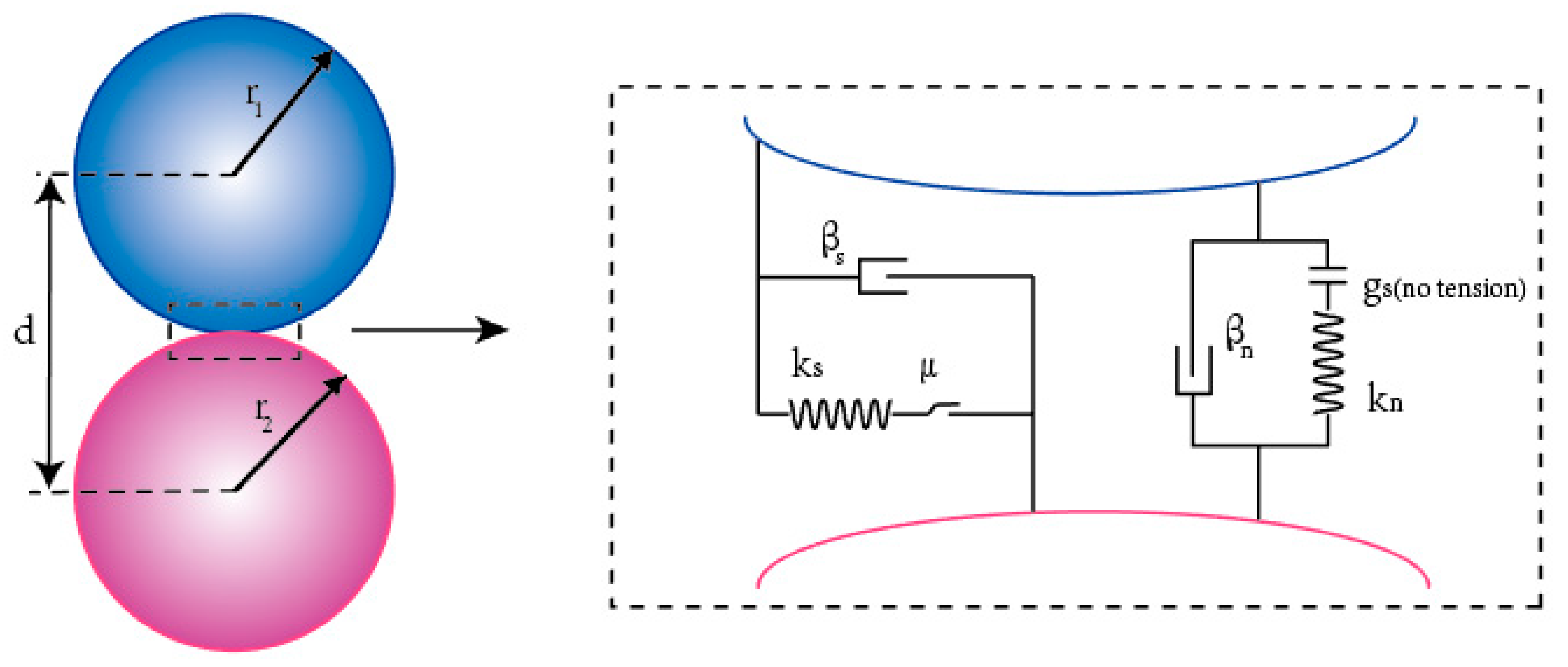
The interaction between particles utilizes a linear contact model established in [32]. The linear contact model decomposes the contact force into a linear component and a damping component. The linear component simulates the linear elasticity and friction characteristics between the materials, whereas the damping component simulates the viscous characteristics of the material [33], as shown in Figure 1. In the Figure 1, kn and ks are the normal and shear stiffness of the linear component, respectively, βn and βs are the normal and shear critical damping ratios of the dashpot component, respectively, μ is the friction coefficient, and gs = d − (r1 + r2), where gs is the surface gap.
The simulated material used in this study is non-cohesive sand; thus, the damping part of the model was not considered. We decomposed the contact force between the particle surfaces into the normal force and the shear force (the same is true for the contact between the particles and the wall); therefore, the contact force between the particles is calculated as follows:
where and are the normal and shear forces at the contact surface ( is tension), respectively, and is the normal direction of the contact plane.
The linear part of the linear model uses a linear spring, with a constant normal stiffness and shear stiffness , to describe the constitutive mechanical behavior of the interparticle contact. The formulas for calculating and are as follows:
where is the calculated shear force, is the initial shear force, is the relative shear-displacement increment, and is the force of friction and the maximum shear force at the contact. The linear stiffnesses, and , and the friction coefficient, , of two contact faces are inherent characteristics of the spring.
For example, the normal stiffness and shear stiffness between two contact surfaces are calculated as follows:
where a and b denote the properties of surfaces a and b that are in contact with each other, respectively. The friction coefficient between faces a and b uses the minimum friction coefficient between the two contact faces: .
The deformability of homogeneous and isotropic materials is generally described using the Young’s modulus () and the Poisson’s ratio (); thus, DEM uses the effective modulus () and the normal-to-shear stiffness ratio () to describe the material deformation capability. The parameters and are linearly related to and , respectively [23]. The effective modulus is calculated using the following formula:
This method can automatically consider the size effect of the particles and adjust the normal and shear stiffness in real time, based on variations in the particle size, making the calculation result more accurate.
2.2. Fluid Component
The fluid calculation component uses the coarse mesh method, where the fluid domain is divided into fluid cells of equal volume. Each fluid cell contains a series of PFC particles, as shown in Figure 2. We used the fluid solver (FiPy) to solve the fluid-flow equation for each fluid element, and we calculated the parameters, such as the velocity and the pressure gradient, of the fluid domain. This study uses the incompressible Navier–Stokes (N–S) equations to obtain the solution. For porous media seepage, the fluid can only flow through the pores, and there is no flow on the part occupied by the solid particles. For convenience during calculation, we used is the porosity of the fluid element and is the macroscopic velocity vector of the fluid element) instead of the seepage flow velocity in the porous medium. The fluid control equation is given as follows:
where is the fluid density, is the element pressure gradient, is the dynamic viscosity of the fluid, is the particle resistance exerted on the fluid, and represents the nabla operator.
The fluid equation uses the porosity term to indicate the presence of particles. There are two methods for calculating the porosity of a fluid cell in PFC, namely, the central method and the polyhedral method [23]. The central method considers that, when the center of the particle is in a fluid element, the particle is completely contained in the fluid element. The polyhedral method uses a cube to characterize a particle whose length, width, and height are equal to the particle diameter. The cell porosity is calculated by determining the overlap volume of the fluid element and the cube. Compared with the central method, calculations performed using the polyhedral method are slower; however, when the particles move between fluid elements, the porosity transition calculated using the polyhedral method changes smoothly. Thus, in this study, we used the polyhedral method to calculate the cell porosity.
We used the element average volume force to calculate the resistance of the particles to the fluid element. We calculated the resistance of the fluid element by summing the fluid drag forces acting on the particles in the fluid element and dividing by the volume of the fluid element:
where the sum is over all the particles in a given fluid element, is the volume of that element, and is the drag force of fluid acting on a single particle.
The fluid forces experienced by the particles include the fluid-to-particle drag force , the fluid gradient force , and the buoyancy .
The drag force of the fluid on the particles is related to the fluid conditions of the element in which the particles are located. Sometimes a particle is located in multiple fluid cells. In this case, the fluid drag force is calculated based on the proportion of particles in the fluid element. The fluid drag force acts on the centroid of the particle regardless of the bending moment. Di Felice [34] showed that the fluid drag force experienced by particles is related to the concentration of the surrounding particles, which is a function of the porosity. In [34], was defined as follows:
where is the fluid drag force on a single particle (in the absence of other particles, ) and is the porosity of the fluid element where the particle is located. The term represents the empirical coefficient of local porosity and is suitable for both high- and low-porosity conditions.
The fluid drag force can be expressed as follows:
where is the coefficient of fluid drag force, is the particle’s velocity vector, and is the radius of the particle.
The coefficient of fluid drag force, , is related to the Reynolds number of the particle, and it is calculated as follows:
where represents the Reynolds number of the particle. The Reynolds number is a dimensionless parameter, representing the motion characteristics of particles in the fluid, and it is defined as follows:
The variable, , in the porosity correction term, , is defined as follows:
The fluid gradient force is calculated as follows:
The buoyancy of a particle is defined as follows:
2.3. Coupling Process
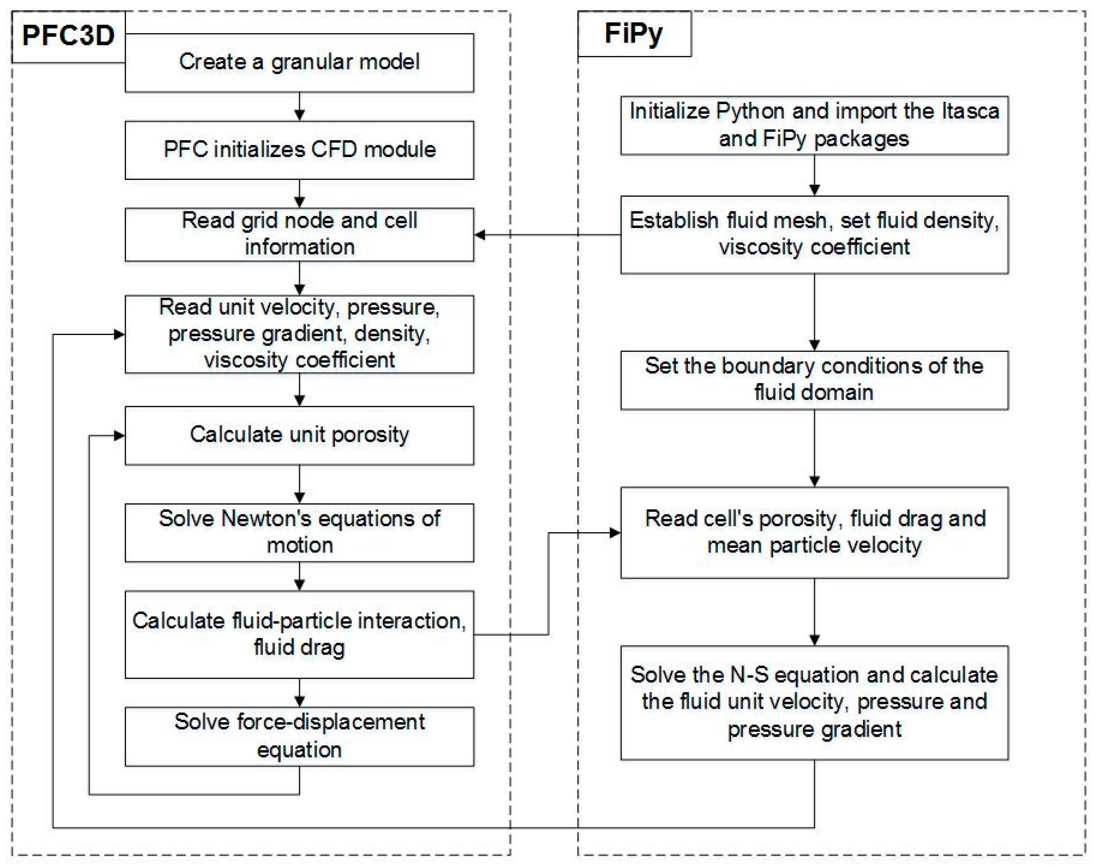
During the coupling process, PFC software was used to solve the equations of the particle motion, and CFD was used to solve the equations of the fluid motion. PFC updates the velocity and position of the particles by measuring the contact between the particles, and Newton’s second law was applied to calculate the force and displacement of the particles. After activating the CFD module, the average volume force of the fluid element and the average velocity of the particles were calculated, and the momentum exchange term was used to solve the fluid motion. The coupling mode and information exchange process are shown in Figure 3. Exchange of information between the two modules needs to be explicitly completed in the PFC data file. First, we used PFC to establish a solid particle model, and then we used the CFD module to establish a fluid grid and set the fluid parameters. PFC was used to read the fluid element information, solve the equation of motion, calculate the element porosity and the average volume force of the fluid elements, and send this information to the CFD module. The CFD module then solves the N–S equation, calculates the fluid element velocity and pressure, and returns them to the PFC. The above process is repeated until the termination condition is met.
3. Modeling
To verify the applicability of the above numerical model, we compared the results obtained by using the numerical model with those of the experimental model. We established experimental and numerical models, as described below.
3.1. Experimental Model
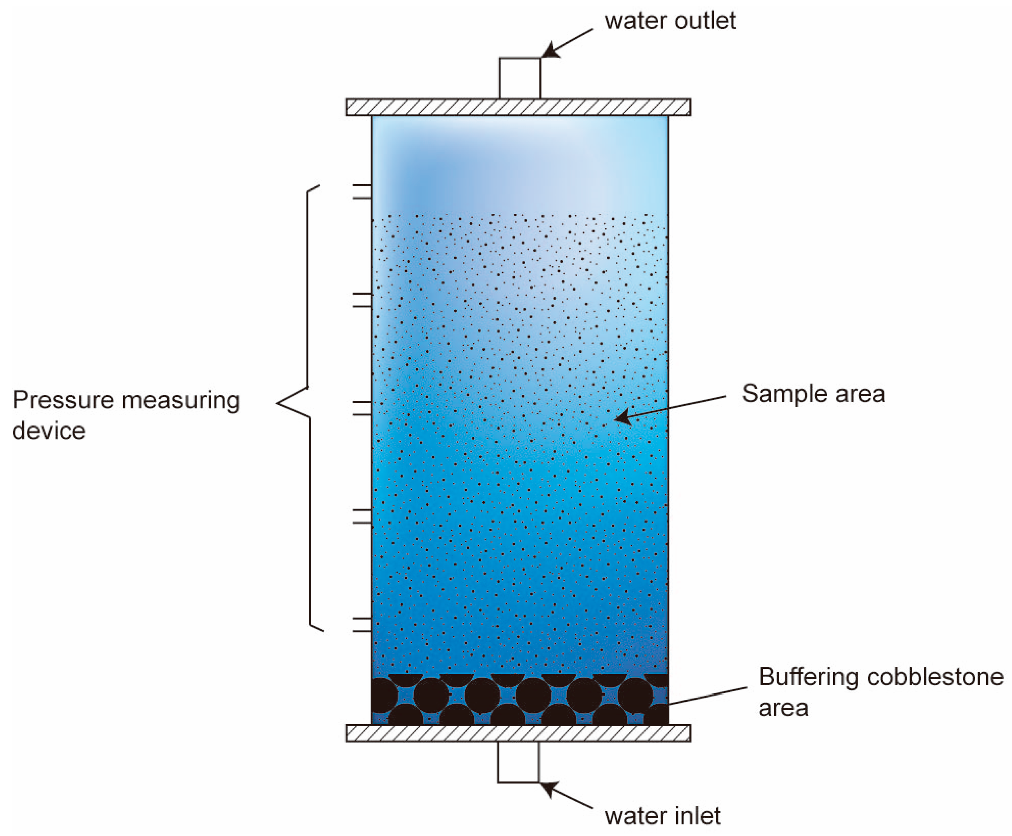
As shown in Figure 4, the internal erosion tests were set up in a cylindrical plexiglass barrel with a diameter of 0.1 m and a height of 0.3 m. The bottom of the plexiglass barrel has a water inlet, and the top of the plexiglass barrel was connected to the water outlet. The water inlet was connected to a flowmeter. The left side of the plexiglass barrel was connected to piezometric tubes. A layer of pebbles with a thickness of approximately 0.04 m was placed under the plexiglass barrel as a buffer zone, so that water could flow into the experimental sample area evenly. For the experimental samples, we used 5–10 mm of coarse sand as the skeleton particles, and 0.5–1.0 mm of standard sand as the filler particles. The skeleton particles and the filler particles were arranged in the ratio of 4:1 by mass. The sample porosity was approximately 0.23.
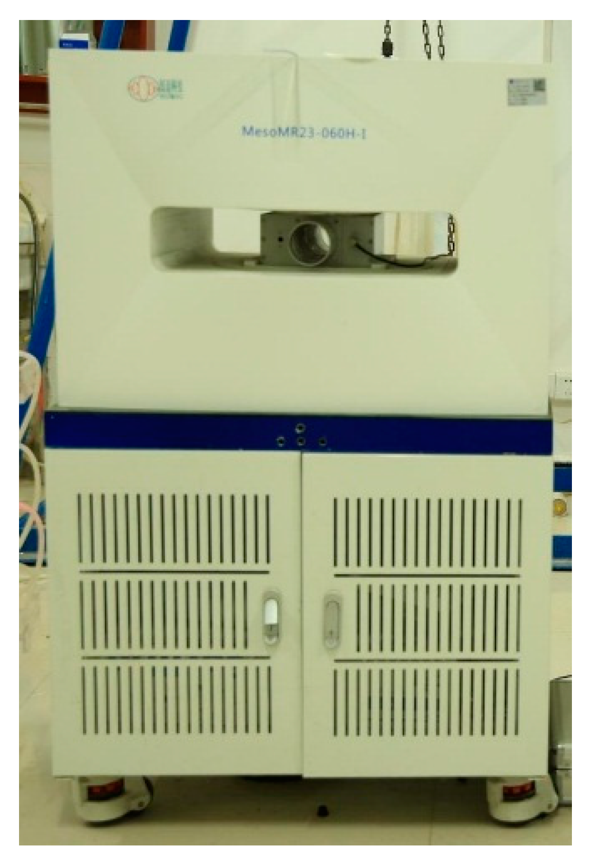
The experimental process is as follows: (1) Place the sand sample into the glass bucket evenly and compact the sand sample layer by layer; (2) add water to the sample and set it aside for 24 h, to ensure that it saturates under natural drainage conditions; (3) adjust the height of the water tank, to ensure that the experimental water head increases in stages; (4) record the readings on the piezometric tube and flowmeter under each head. When the sample is stable, quickly place the sample into the nuclear magnetic resonance (NMR) device, to measure the porosity, as shown in Figure 5; (5) repeat the third step continuously, until the sample is destroyed.
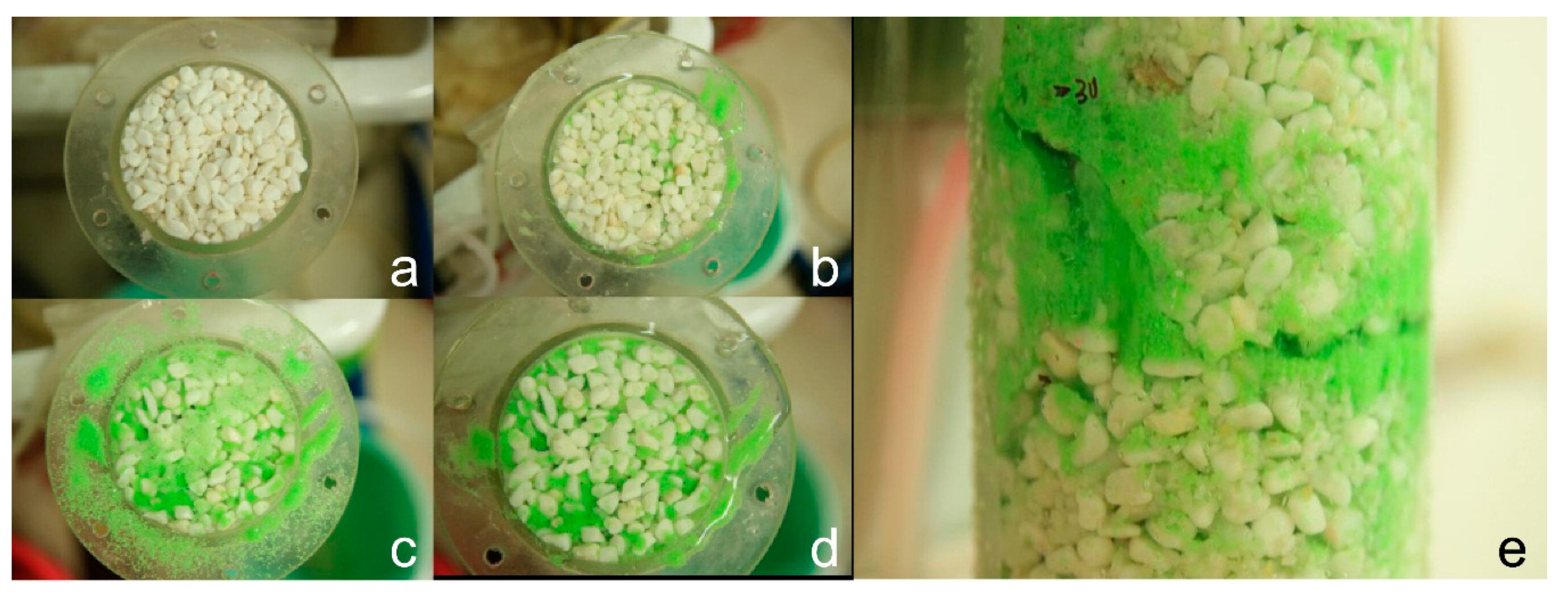
Under the same test conditions, we performed seepage experiments on multiple groups of samples, to avoid accidental errors in the experimental results. The duration of each test was 240 min. The experimental results are shown in Figure 6. At the beginning, the experimental sample was stable, and no obvious particle movement was observed, as shown in Figure 6a. The experimental water head increased, and some fine particles were transported by water flow. However, most of the fine particles were still trapped under the skeleton particles, as shown in Figure 6b. The experimental water head continued to increase, and many fine particles burst out of the gap, as shown in Figure 6c. With the increase in the water head, the skeletal particles loosened, and the sample moved upward, as a whole, as shown in Figure 6d,e.
3.2. Numerical Model
We developed a numerical model based on the experimental model. We did not establish a numerical model that is 1:1 with the experimental model, due to the limitations of the computing power. For example, a sand sample with a size of 0.1 m × 0.1 m × 0.2 m contains approximately 1 million particles. Presently, the computer capacity for this calculation is still insufficient. Thus, to make the analysis feasible and effective, the number of model particles should be reduced. We simplified the numerical model in terms of both the model size and the particle size. We developed a numerical model with a diameter of 40 mm and a height of 80 mm, which is approximately 6.4% of the test model. In PFC, maximum to minimum particle size () ratios has a great influence on the calculation efficiency. The larger maximum-to-minimum particle-size ratio, the slower the calculation speed [35]. Thus, we generally control the particle size ratio to within 10. In this study, the particle size ratio for the experimental model was too large. To obtain a reasonable calculation efficiency, we used the median value of the particle size range of the control particles and the filler particles as the representative particle size. Thus, we used 7.5 mm for coarse particles and 0.75 mm for fine particles.
We first generated the sample container. We used three fixed and impenetrable walls as the container for the sample. The top and bottom of the container consisted of two square walls, with a cylindrical wall on the side. In the PFC model, the sand was modeled as a complete sphere, and the model considered the friction between the particles but did not consider the effect of the shape of the particles. Numerical simulation typically employs the Young’s modulus to study the mechanical behavior of sand. The Young’s modulus for natural gravel is approximately 70–170 MPa. In PFC, we used the effective modulus, which is proportional to the Young’s modulus; thus, the effective modulus used in this study is 100 MPa. The true coefficient of friction of sand is typically 0.5–0.7 [36], but after the addition of fluid, the sliding friction of the particles decreased significantly [37]; thus, the friction coefficient used in this study is 0.5.
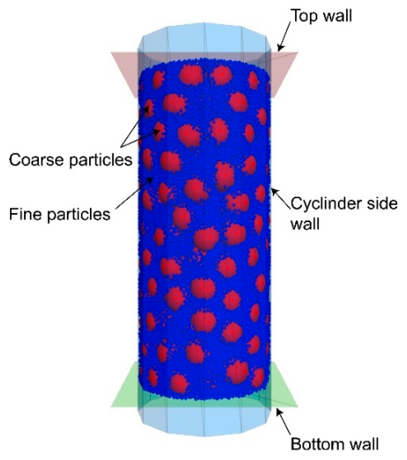
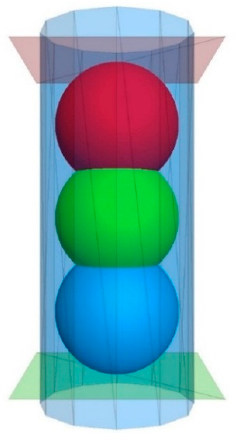
Next, we filled the inside of the container with particles. Similar to the experimental model, the mass percentage of coarse and fine particles was 4:1. Assuming that the density of the gravel is uniform, the coarse and fine particles’ volume percentage is also 4:1. We generated a sample model based on particle grading, setting the initial porosity to 0.3 (the initial model ball particles overlap and the porosity will decrease after the particles bounce, so we set the initial porosity to be larger), whereas the coefficient of friction was set to 0.5. We limited the amount of overlap to 0.1, using the control function as the particles of the initial model have a large overlap. We then eliminated the imbalance between the particles by a cyclic calculation, to generate a stable model that contains 41,031 particles, as shown in Figure 7. In numerical simulation, we needed to monitor the evolution of the model state and the parameters, to determine the variation law of the microscopic features and the parameters of the model. Thus, we established three equal-volume measurement regions for monitoring and recording the porosity of the model. We set the measurement region to a sphere. The radius of the spherical measurement region is 16 mm, and the center of the three measurement regions is on the central axis of the cylindrical model, as shown in Figure 8. We numbered the three spherical measurement regions from top to bottom, with the red area numbered as 1, the green area numbered as 2, and the blue area numbered as 3.
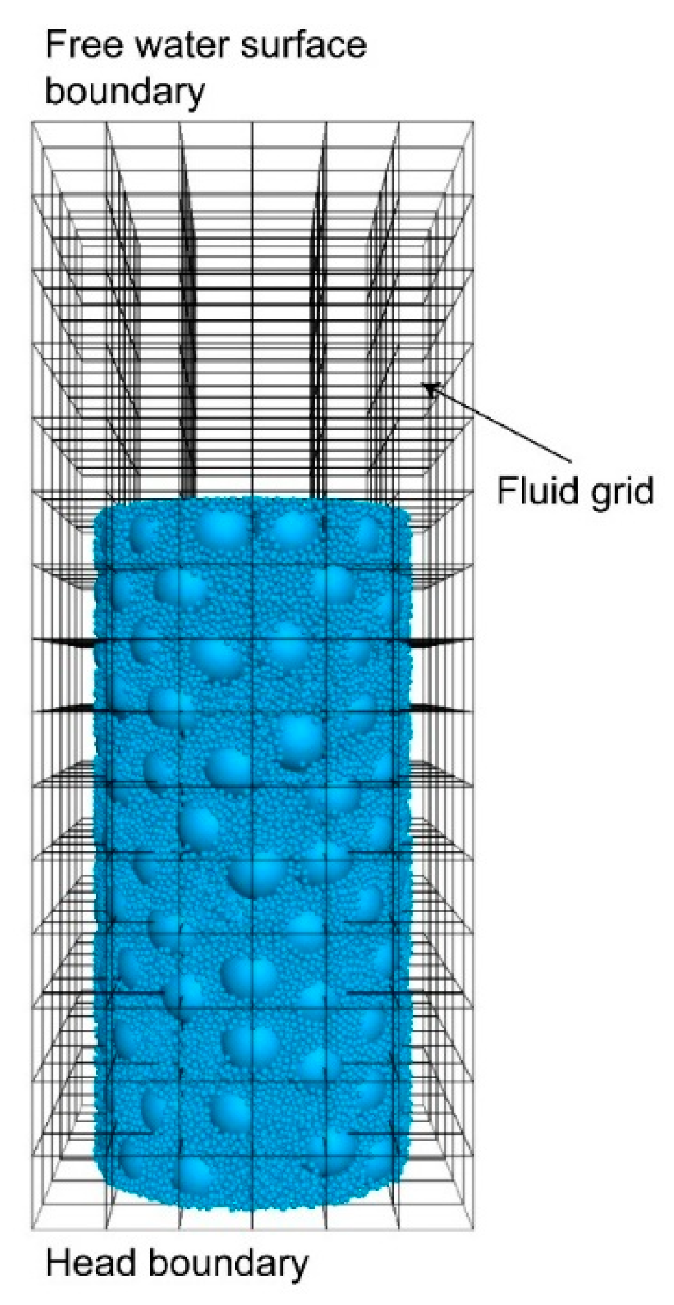
We developed a fluid mesh based on this particle model. We used a series of equal-sized hexahedral grid elements to describe the fluid region, as shown in Figure 9. At the same time, we removed the top wall of the particle model. The grid element size is 8 mm × 8 mm × 8 mm, and the number of grid elements is 540. We set the fluid to move from bottom to top and also set the fluid-pressure boundary conditions. The fluid outlet pressure is zero, and the inlet head of the fluid increases with the calculation time. The fluid side boundary is an impermeable boundary condition, and hence there is no radial seepage.
The position of the particles was calculated based on the time increment, as the PFC predicts the displacement of the particles according to Newton’s second law. The stable step size of the PFC is very small, generally 100 ns; thus, it is difficult to make the calculation time consistent with the actual experimental time. To improve calculation efficiency, we reduced the computation time by increasing the pressure gradient. Zheng et al. [29] concluded that the higher hydraulic gradient contributes to the evolution rates of both volumetric contraction and void ratio. It also has been reported that increasing the pressure gradient does not affect the stability of the model because the fluid motion is calculated by using the N–S equation [38]. Therefore, we put forward the assumption that an increase in the hydraulic gradient can accelerate the material behavior of the sample. To test this hypothesis, we compared the evolution in porosity and seepage velocity of the same model under different hydraulic gradients.
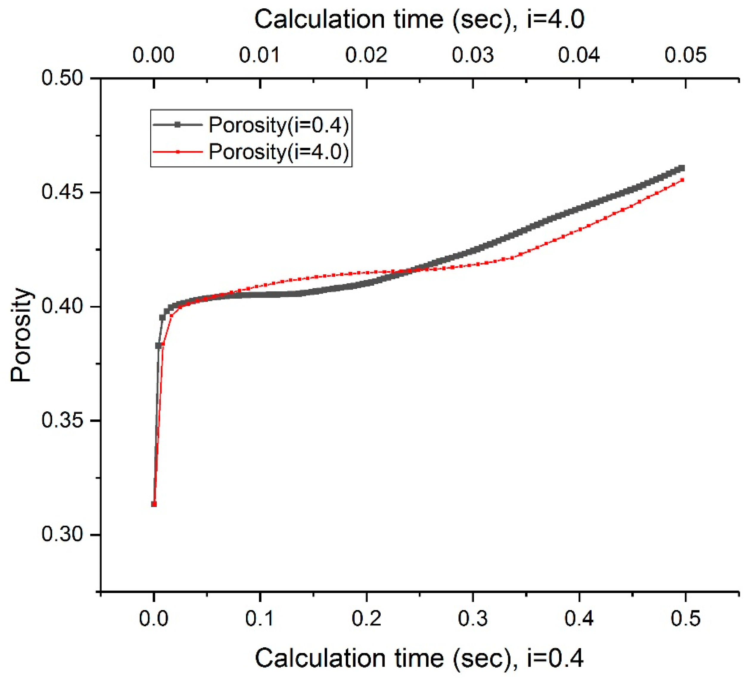
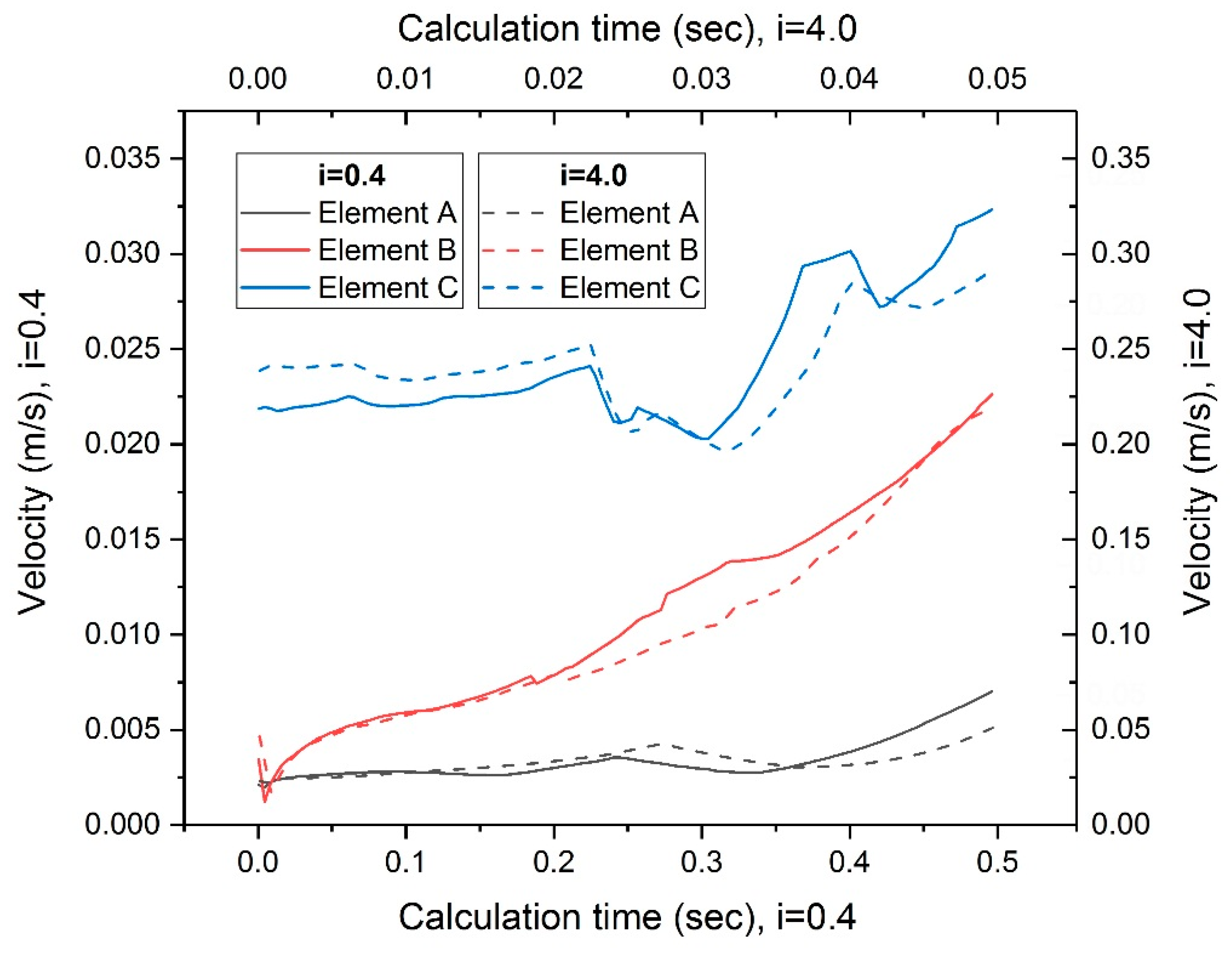
We built a numerical model with fewer particles for testing, which is based on the prototype numerical model. The test numerical model is a cylinder with a diameter of 0.02 m and a height of 0.04 m. It contains 4609 particles and has an initial porosity of 0.35. The size of the fluid element is 5 mm × 5 mm × 5 mm, and the test numerical model contains 300 elements. The other parameters of the test numerical model are the same as the prototype numerical model (refer to Table 1). Two scenarios with different hydraulic gradients of the test model are simulated (i.e., I = 0.4, calculation time = 0.5 s, and i = 4.0, calculation time = 0.05 s). The results are shown in Figure 10 and Figure 11.
After increasing the hydraulic gradient, the porosity of the test model did not change much, as shown in Figure 10. During the test, we randomly selected 3 fluid elements and recorded the evolution of the seepage velocity of the three fluid elements under different hydraulic gradients, as shown in Figure 11. Increased hydraulic gradient increased seepage velocity but did not affect the trend of seepage velocity. Therefore, our hypothesis is feasible.
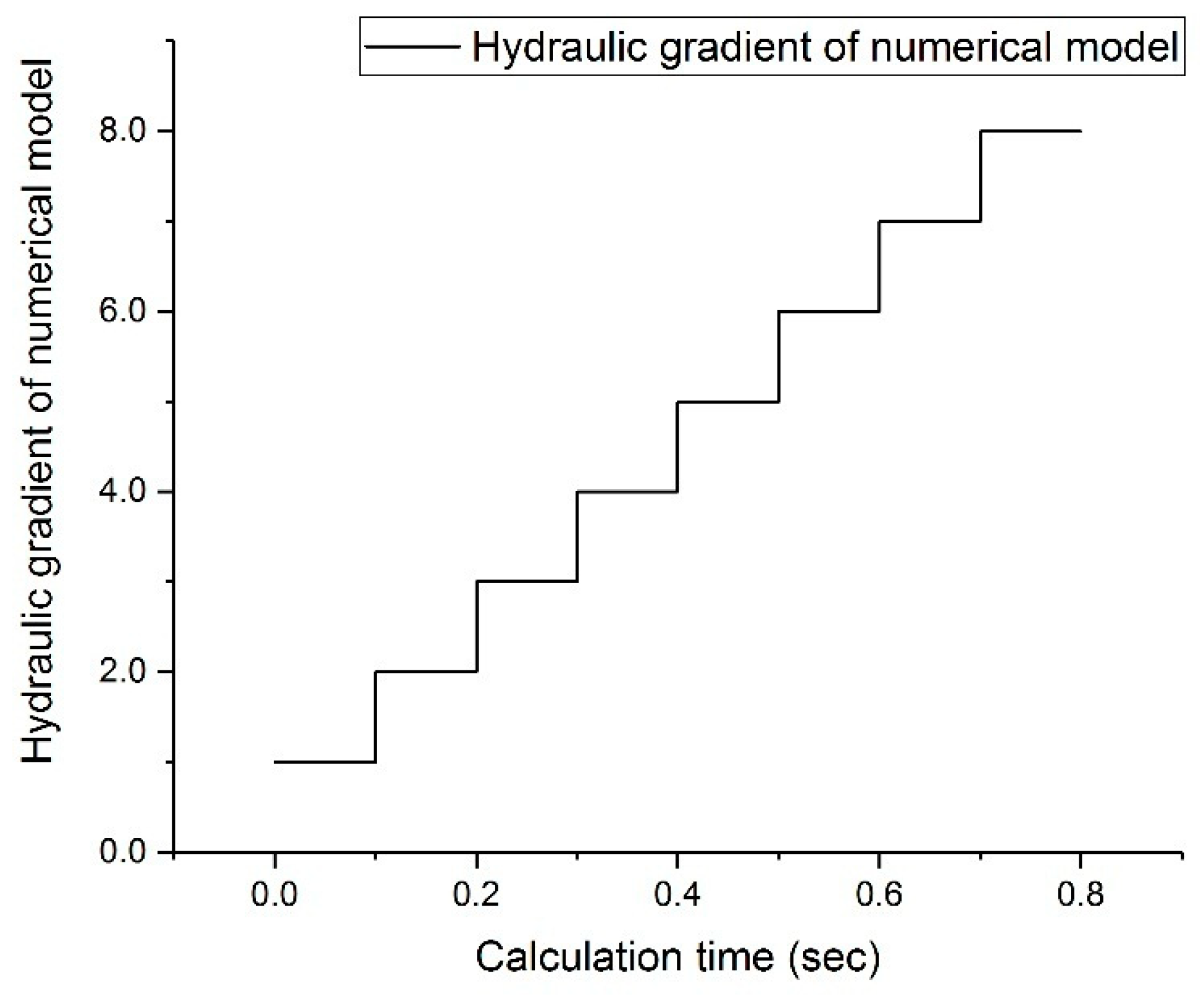
In this study, we calculated the hydraulic gradient as 10 times compared with the experimental model. Thus, we set the initial inlet hydraulic gradient to 1.0 and increased stepwise at a rate of 10 s−1, as shown in Figure 12. The time step calculated by the particle model is taken as 200 ns, and the time step of the fluid model calculation is taken as 20 μs. Thus, for every 100 steps of the particle model calculation, the fluid model was calculated in one step and information was exchanged once. Other parameters of the model are listed in Table 1.
4. Results Analysis
4.1. Model Verification
To verify the performance of the developed numerical model, we analyzed and compared the experimental results and numerical results. In the experiment, when the hydraulic gradient was 0.38, the surface of the sands model suddenly appeared to have a large area of sand boil, and the water pressure measured by a piezometer suddenly dropped. This phenomenon indicates that the sands model underwent seepage failure. Therefore, we define 0.38 as the critical hydraulic gradient of the experimental model, expressed as (for ease of differentiation, we used to represent the hydraulic gradient of the experimental model, and to represent the hydraulic gradient of the numerical model).
Figure 13 shows the evolution of the outlet water velocity with the hydraulic gradient of the experimental and numerical models. In the experimental model, it can be observed that the velocity increases linearly with the hydraulic gradient before , which is consistent with Darcy’s law of flow. When , the velocity of the experimental model shows a sudden increasing trend. The velocity changes from linear to nonlinear with the change in the hydraulic gradient, which verifies the state change from laminar to turbulent flow when seepage failure occurs in the sands model. The velocity-change trend of the numerical model is essentially the same as that of the experimental model. The velocity change of the numerical model is also stepwise, as its hydraulic gradient is stepwise. The difference is that the velocity of the numerical model exhibits nonlinear growth after (t = 0.3–0.4 s), hence we define the critical hydraulic gradient of the numerical model as 4.0: .
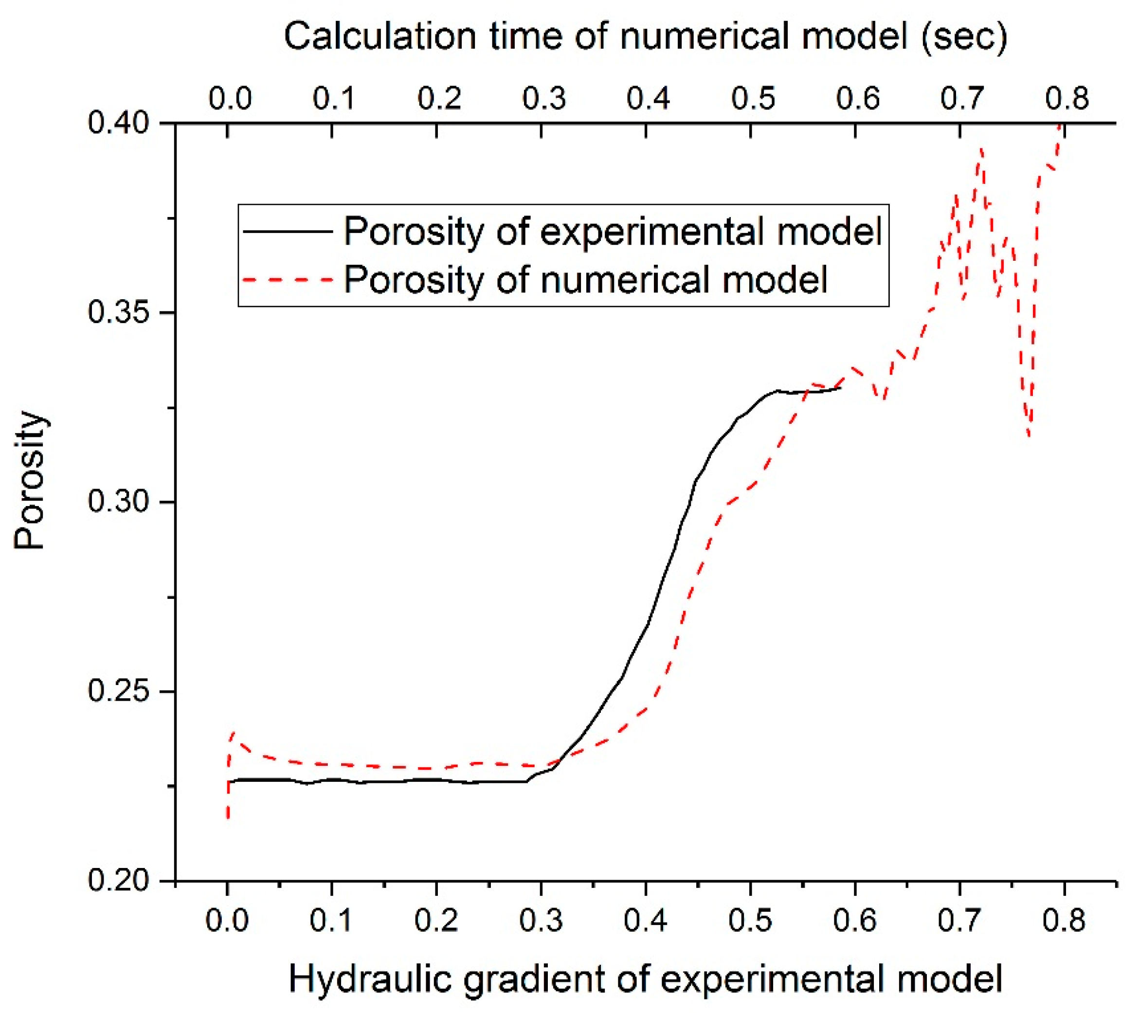
In the experimental model, we monitored and recorded the porosity at the middle of the sample. In the numerical model, we also recorded the change in the average value of the porosity of several fluid elements located in the middle of the sample, based on geometric similarity. Figure 14 shows the difference in the porosity of the experimental and numerical models under different hydraulic gradients; the result of the experimental model roughly correlates with that of the numerical model. The porosity of the two models remains unchanged under a low hydraulic gradient. When or (t = 0.2–0.3 s), the porosity begins to increase slowly due to loss of fine particles, whereas the porosity begins to change significantly at approximately or . The porosity of the experimental model tends to be stable at . However, the porosity of the numerical model continues to increase.
From Figure 13 and Figure 14, we can conclude that, when (t = 0.0–0.6 s), the numerical simulation results can reproduce the trend of the mesoscopic parameters of the piping well. The change in porosity is important for the evolution of fluid velocity, and a larger porosity results in a larger fluid velocity. When (t = 0.6–0.8 s), the results of the numerical simulation are significantly different from the experimental results. We attribute the difference to two aspects.
The first is the effect of size effects. The numerical model is approximately 6.4% of the experimental prototype and the number of particles in the numerical model is small. After the occurrence of seepage failure in the model, the percentage of particle loss in the numerical model is much larger than the experimental model. The porosity of the numerical model increased rapidly. The seepage velocity is related to the porosity, so the seepage flow velocity also changes greatly. Seepage failure has a greater impact on the numerical model, and the second is the effect of the choice that we multiply the hydraulic gradient by a factor 10 compared to experimental conditions. Internal erosion is a process from linear to nonlinear. When seepage failure occurs, the relationship between velocity and hydraulic gradient changes to nonlinear. Therefore, the velocity change of the numerical model is larger than the test velocity. The particles in numerical model moved faster, and the porosity also changed greatly.
4.2. Particle Migration and Changes in Contact Force
The calculation step of this model requires 200 ns, and a total of four million steps were calculated. The simulation results demonstrate the occurrence and development of internal erosion. Figure 15 and Figure 16 show the variation of particle displacement and contact force of the model under different hydraulic gradients. We categorized the process into five stages.
4.2.1. Particle-Consolidation Stage
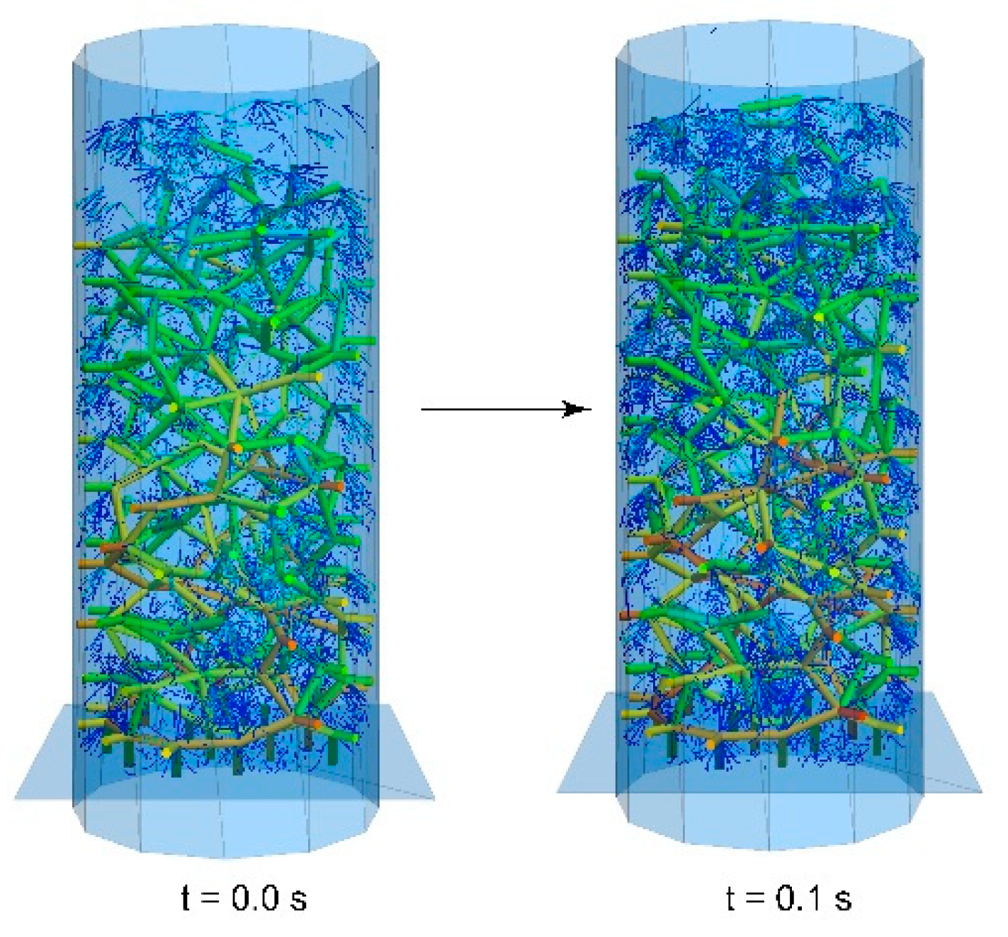
This stage occurs when the hydraulic gradient . At the beginning of the calculation, fluid force and gravity were simultaneously applied to the particles, the hydraulic gradient increased from 0 to 1.0, and the particles started moving under the action of gravity and fluid force. At this time, the gravity of the particles is greater than the fluid force, and the sample model is consolidated and sedimented. As shown in Figure 17, the average porosity of the model calculated based on the measurement region is continuously decreasing during the calculation time of 0 s to 0.1 s (), indicating that the model is consolidated under the hydraulic gradient of 1.0. Figure 18 shows the contact force of the model in the calculation time of 0.0 s to 0.1 s; the increase in the number of model contacts can be clearly observed. The longer cylinders represent contact between the skeleton particles, and between the skeleton particles and the wall, whereas the relatively shorter cylinders represent contact between the filler particles, and between the filler particles and the wall. In the process of particle consolidation, the fine particles settle under the action of the external force from the point of contact bonds, and the mechanical structure between the skeleton particles is almost never unchanged. From the color change of the contact bonds, the contact force between the skeleton particles slightly increased. This is due to the consolidation of the fine particles, which increases the pressure on the skeletal particles, but the consolidation of the particles does not affect the main mechanical structure of the model. At this time, the contact force between the particles starts increasing, and the force is uniformly distributed on all the particles when it is transmitted between the skeleton particles. As the depth of the model increases, the contact force between the skeleton particles also gradually increases.
4.2.2. Loss Stage of Fine Particles
This stage mainly occurs when and . As the hydraulic gradient gradually increases, the fluid force of the fine particles gradually increases and exceeds gravity. Next, the fine particles begin to move upward. As shown in Figure 17, when the hydraulic gradient increases to 2.0 (t = 0.1–0.2 s), loss of fine particles begins at the outlet of the model, and the average porosity of the model rises slowly. The hydraulic gradient at this time does not have a large effect on the model. When the hydraulic gradient increases to 3.0 (t = 0.2–0.3 s), the porosity of the model increases, and a large number of fine particles are lost in the model outlet, as shown in Figure 15. As the filler particles have been lost, the contact force between the particles has changed. The number of contacts between the particles and magnitude of contacts in the model are significantly reduced, as shown in Figure 16. The loss of fine particles at this stage is an important prerequisite for the occurrence of seepage failure of the soil, marking the beginning of the formation of a leakage channel.
4.2.3. Loosening Stage of Skeleton Particles
This is also the stage in which internal erosion begins to occur, which starts when . The increase in the hydraulic gradient causes the external force of the skeleton particles to tend to zero, and then the skeleton particles begin to loosen. The hydraulic gradient at this time is known as the critical hydraulic gradient. With the increase in the hydraulic gradient and increase in the loss of fine particles in the previous stage, the porosity of the model increases, and the fluid velocity increases gradually. The fluid force of the skeleton particles becomes gradually greater than gravity. At this time, the skeleton particles at the outlet of the model have been loosened and begin to move upward. As shown in Figure 15, the model structure has been destroyed, and a seepage channel first forms at the outlet of the model, that is, seepage failure begins. As shown in Figure 16, the contact force structure between the particles at the exit is significantly damaged.
4.2.4. Volume-Expansion Stage
With the gradual loss of particles, erosion continues to propagate downward, and the skeleton particles move slowly toward the outlet. Next, the overall porosity of the model increases, and the model volume begins to expand. This stage occurs when and (t = 0.4–0.6 s). The number of contacts between the particles is reduced, and the mechanical structure is further destroyed. The contact force between the particles increases slightly owing to the increase in the hydraulic gradient, and the fluid force of the particles increases and is evenly distributed on the particles; thus, the pressure of the particles increases, which manifests as an increase in the contact force.
4.2.5. Overall-Ascending Stage of Soil
As shown in Figure 15 and Figure 16, when and , the bottom layer of the model particles is under the action of gravity of all the particles in the upper layer. As the upper layer particles move gradually, the pressure on the bottom layer gradually decreases. Further, as the hydraulic gradient increases, the bottom layer particles begin to move upward. At this stage, the number of contacts between the model particles continues to decrease, and the contact force increases as the hydraulic gradient increases.
4.3. Evolution of Porosity
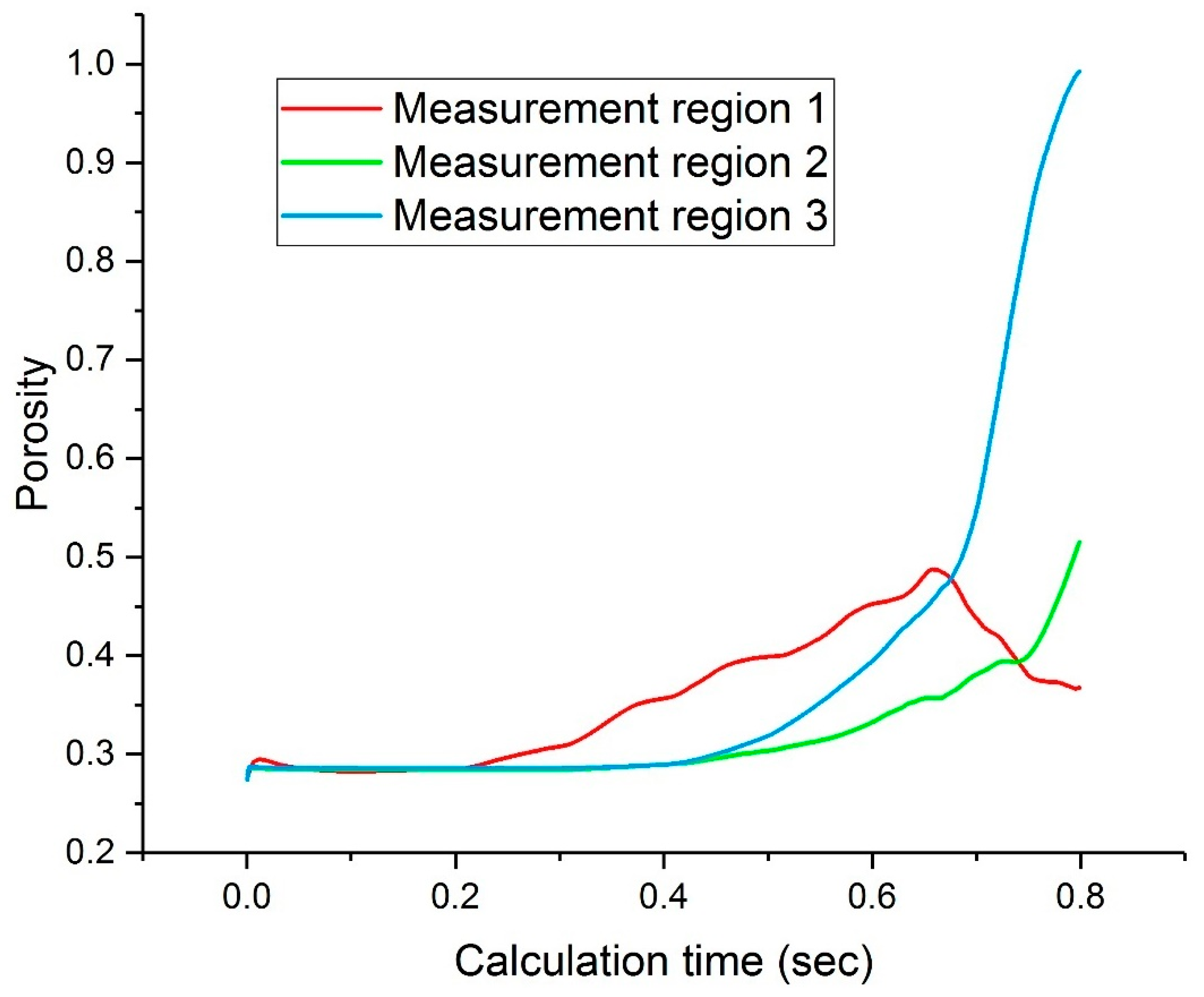
The evolution of porosity is closely related to the movement of particles during the internal erosion process. We have established three measurement regions, from top to bottom (Figure 8), and recorded the evolution of porosity, as shown in Figure 19. Measurement region 1 is close to the model outlet, and loss of fine particles occurs (stage 2). Thus, the porosity of measurement region 1 changes first. When t = 0.3 s (), the porosity growth rate of measurement region 1 increases, and internal erosion begins to occur. When t = 0.4 s (), the porosity of measurement regions 2 and 3 begins to increase. The model is then in the volume expansion stage, and internal erosion has moved into the lower part of the model. The porosity of measurement region 3 changes the most. As measurement region 3 is at the bottom of the model, the particles continuously move from measurement region 3 to measurement region 2. The number of particles in measurement region 3 gradually decreases, and, finally, the porosity increases to 1.0, as the number of particles in this region decreases to zero. The porosity of measurement region 2 changes minimally, indicating that the number of particles in this region is essentially constant. Although the particles in this region gradually move to measurement region 1, the region also continuously receives particles from measurement region 3. When the model is in the volume expansion stage (stage 4, t = 0.4–0.6 s), the porosity of measurement region 2 increases slightly. When the erosion develops to the overall ascending stage (t = 0.7–0.8 s), the porosity of measurement region 2 begins to increase substantially. At this stage, the number of particles received in measurement region 2 is much smaller than the number of particles lost. At this point, the porosity of measurement region 1 begins to decrease. Many particles infiltrate into measurement region 1 due to the overall upward movement of the model. Further, the number of particles received in measurement region 1 exceeds the number of particles lost; thus, the porosity of measurement region 1 increases. The evolution of porosity directly reflects the change in particle loss at different locations of the model.
4.4. Evolution of Particle Velocity and Mass-Loss Measurement
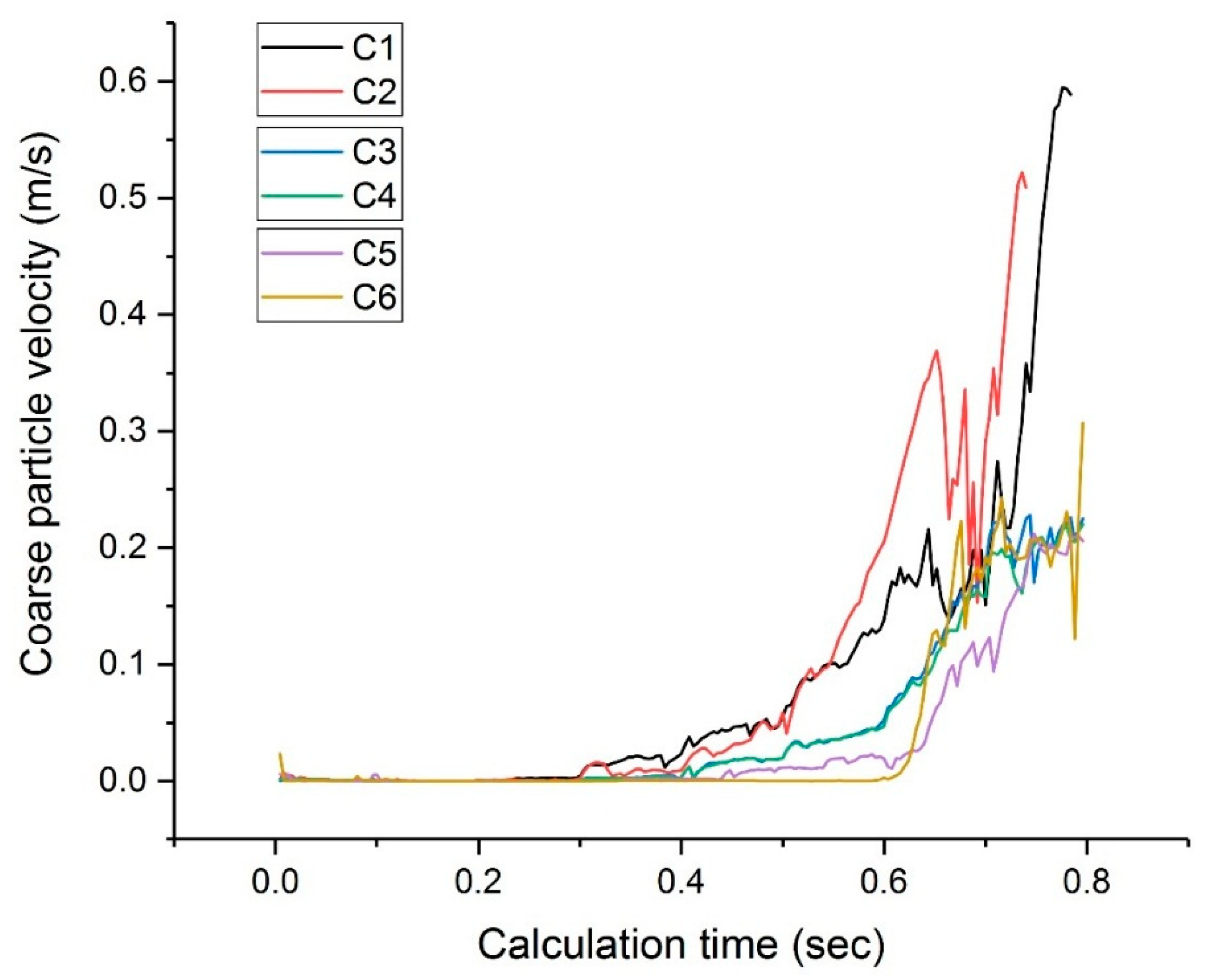
We divided the model evenly into three layers and defined these as the top, the middle, and the bottom layers. Two coarse particles and two fine particles were randomly selected in each layer. We then recorded the velocities of the 12 particles. Figure 20 and Figure 21 show the velocity changes of the coarse and fine particles in different layers.
The velocity of particles in the top layer changes first, and then it begins to increase significantly around the critical hydraulic gradient of 4.0. The velocity of the middle layer particles starts to increase slowly near the critical hydraulic gradient of 4.0, and it increases significantly during the overall ascending stage. The particle velocity of the bottom layer begins to change significantly during the overall ascending stage. Finally, the velocity of the middle and bottom skeleton particles is stable at approximately 0.18 m/s, and the speed of the fine particles fluctuates at approximately 0.2 m/s. As shown in Figure 20, the top skeleton particles, C1 and C2, decrease in velocity after 0.6 s, at which time the two skeleton particles may be clogged. Furthermore, after 0.7 s, the velocity rises, and clogging is eliminated. The skeletal particles are slightly affected by fluctuation in water flow, and the velocity increases smoothly. The filler particles’ weight is low, and it is significantly affected by fluctuation in water flow. The filling particles’ velocity fluctuates significantly.
At t < 0.3 s (), the fluid velocity is small, and the velocity of the skeleton particles is always zero. At t = 0.3 s (), some of the skeleton particles start moving. The velocity of the top skeleton particles (C1 and C2) changes first. At the beginning, the velocity of the skeleton particles (C1 and C2) changes minimally, and it fluctuates at 0.025 m/s. At this time, seepage failure occurs, and the model outlet initially forms a leakage channel. The velocity of the top skeletal particles begins to increase significantly at t = 0.4 s (), and it continues to increase with the hydraulic gradient, until the particles are flushed out of the model. The velocity of the middle skeleton particles (C3 and C4) increases slowly from zero after t = 0.4 s (), and it increased after t = 0.5 s (), indicating that internal erosion has moved to the middle of the model. The velocity of C5 starts fluctuating slightly at t = 0.4 s (), and the C6 particle velocity is zero. At t = 0.6 s (), the velocity of C5 and C6 suddenly increases, and the degree of erosion increases. At t = 0.7 s (), the velocity of the middle and bottom layer particles is approximately the same, and it fluctuates at 0.2 m/s. The model is in the overall ascending stage.
The rate of change of the velocity of the fine particles is approximately the same as that of the coarse particles. However, the initiation hydraulic gradient of fine particles is lower than that for coarse particles such that the fine particles are more likely to move. The velocity of the fine particles starts fluctuating slightly at t = 0.1 s (). When the model is stable, the velocity of the fine particles is very small, but its fluctuation is severe. At this time, the soil structure has not been destroyed, and the fine particles are confined in the fixed soil structure and violently jump in the void. As the hydraulic gradient increases, the soil structure gradually loses stability, and the fine particles are eventually moved out of the soil structure.
Chang et al. [39] once defined two critical hydraulic gradients, namely the initiation hydraulic gradient and the skeleton-deformation hydraulic gradient. The initiation hydraulic gradient represents the hydraulic gradient where internal erosion begins, whereas skeleton-deformation hydraulic gradient represents the hydraulic gradient in which the soil structure begins to deform and seepage failure occurs. We can conclude that the numerical model’s initiation hydraulic gradient is 2.0, and the skeleton-deformation hydraulic gradient is 4.0.
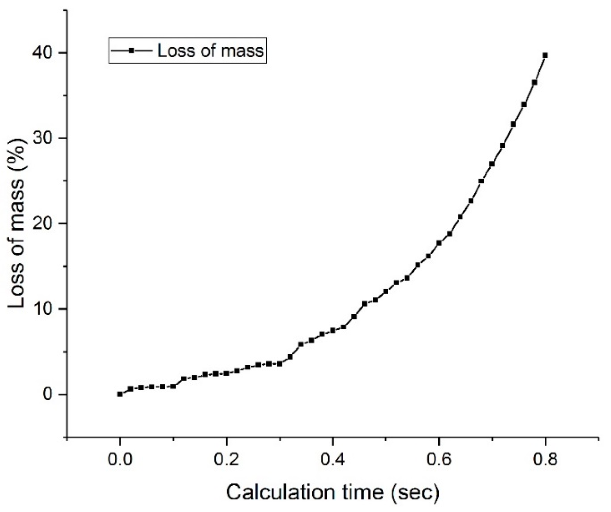
Figure 22 is mass-loss measurement of the numerical model. When t = 0–0.1 s (), the particles on the surface of the model are taken away by the water flow, and the mass loss at this time is small, less than 1%. When t = 0.1–0.3 s (), the hydraulic gradient reaches the initiation hydraulic gradient of the model. The fine particles start to move, and the mass loss increases and gradually stabilizes to 4% over time. When t > 0.3 s (), the hydraulic gradient reaches the skeleton-deformation hydraulic gradient. The skeleton particles start to move under the action of the fluid. A large number of particles is lost, and the mass loss also increases rapidly. These two critical hydraulic gradients, the initiation hydraulic gradient and the skeleton-deformation hydraulic gradient, have important effects on mass loss.
5. Conclusions
In this study, we proposed and established a numerical model to investigate the fluid–solid coupling effect of internal erosion and carried out related experiments. The experimental results and the model results were quantitatively compared to verify the usability of the numerical model. We described the mechanism of the occurrence and development of internal erosion and divided the process of internal erosion into five stages by analyzing the particle migration, contact force, porosity, and particle velocity evolution of the model.
The following conclusions are dawn from the study.
- (1)
- The essence of internal erosion is the gradual loss of soil particles. Piping erosion first destroys the surface layer of soil, and then, as the soil particles are continuously moved away by water flow, the erosion gradually develops into the deep layer of the soil, eventually causing the soil to undergo seepage failure.
- (2)
- An increase in the hydraulic gradient is an important cause of instability of the mechanical structure of the soil. Loss of particles under a low hydraulic gradient does not affect the magnitude and structure of the contact force of the model. However, as the hydraulic gradient increases, the contact force between particles decreases, the mechanical connectivity between particles decreases, and the mechanical stability decreases, eventually resulting in instability of the mechanical structure of the model.
- (3)
- The evolution of porosity is closely related to the migration of particles. The evolution of porosity at different locations can reflect the migration of soil particles.
- (4)
- The initiation hydraulic gradient of the particles is dependent on location. The deeper the particle position, the larger the initiation hydraulic gradient. The initiation hydraulic gradient is also dependent on the size of the particles. The smaller the particles, the smaller the initiation hydraulic gradient.
- (5)
- The initiation hydraulic gradient and the skeleton-deformation hydraulic gradient determine whether the particles will move and have a decisive effect on mass loss.
- (6)
- DEM–CFD coupled numerical simulation can visually show the evolution of particle migration and contact force under different hydraulic gradients. It is an advanced simulation technology that provides a research platform for studying the mesoscopic mechanism of soil seepage deformation. Numerical simulation has become an increasingly useful tool for studying the mesoscopic mechanism of internal erosion.
This study helps people better understand the microscopic mechanism of internal erosion and provides further theoretical guidance on the prevention and control of internal erosion. However, due to the limitation of the DEM calculation, we cannot perform calculations based on real physical time. How to specify the equivalence in physical time between the numerical model and the experiment will be the focus of our future research.
Multiscale modeling is still difficult to achieve. Further, the application of DEM in practical engineering projects is relatively difficult to achieve at present, due to the limitation of its calculation method. It is recommended that future research should investigate how to establish the scale relationship between the model and the actual project.
Author Contributions
Conceptualization, Y.W., J.C., Z.X., and Y.Q.; methodology, Y.W.; software, Y.W.; validation, Y.W.; formal analysis, Y.W.; investigation, Y.W. and X.W.; resources, Y.W. and X.W.; data curation, Y.W.; writing—original draft preparation, Y.W.; writing—review and editing, Y.W.; visualization, Y.W.; supervision, J.C.; project administration, J.C.; funding acquisition, J.C. All authors have read and agreed to the published version of the manuscript.
Funding
This research was funded by the National Natural Science Foundation of China (Grant No. 51679197), the Natural Science Basic Research Program of Shanxi Province-Key Project (Grant No. 2017JZ013), and the Leadership Talent Project of Shaanxi Province High-Level Talents Special Support Program in Science and Technology Innovation (Grant No. 2013KCT-15).
Conflicts of Interest
The authors declare no conflicts of interest.
References
- Fell, R.; Fry, J.J. State of the Art on the Likelihood of Internal Erosion of Dams and Levees by Means of Testing. In Erosion in Geomechanics Applied to Dams and Levees; John Wiley & Sons: Hoboken, NJ, USA, 2013; pp. 1–99. [Google Scholar]
- Bonelli, S.; Benahmed, N. Piping Flow Erosion in Water Retaining Structures: Inferring Erosion Rates from Hole Erosion Tests and Quantifying the Failure Time. In Proceedings of the 8th ICOLD European Club Symposium: Dam Safety – Sustainability in a Changing Environment, Innsbruck, Austria, 22 September 2010. [Google Scholar]
- Foster, M.; Fell, R.; Spannagle, M. The statistics of embankment dam failures and accidents. Can. Geotech. J. 2000, 37, 1000–1024. [Google Scholar] [CrossRef]
- Richards, K.S.; Reddy, K.R. Critical appraisal of piping phenomena in earth dams. Bull. Eng. Geol. Environ. 2007, 66, 381–402. [Google Scholar] [CrossRef]
- Shire, T.; O’Sullivan, C. Micromechanical assessment of an internal stability criterion. Acta Geotech. 2013, 8, 81–90. [Google Scholar] [CrossRef] [Green Version]
- Wang, Y.; Li, C.; Zhou, X.; Wei, X. Seepage piping evolution characteristics in bimsoils—An experimental study. Water 2017, 9, 458. [Google Scholar] [CrossRef] [Green Version]
- Bligh, W.G. Dams, barrages and weirs on porous foundations. Eng. News 1910, 64, 708–710. [Google Scholar]
- Lane, E.W. Security from under-seepage-masonry dams on earth foundations. Trans. Am. Soc. Civ. Eng. 1935, 100, 1235–1272. [Google Scholar]
- Terzaghi, K. Erdbaumechanik auf Bodenphysikalischen Grundlagen; Deuticke: Wien, Austria, 1925. [Google Scholar]
- Rosenbrand, E. Investigation into Quantitative Visualisation of Suffusion. Master’s Thesis, TU Delft, Delft, The Netherlands, 2011. [Google Scholar]
- Moffat, R.; Fannin, R.J.; Garner, S.J. Spatial and temporal progression of internal erosion in cohesionless soil. Can. Geotech. J. 2011, 48, 399–412. [Google Scholar] [CrossRef]
- Sibille, L.; Marot, D.; Sail, Y. A description of internal erosion by suffusion and induced settlements on cohesionless granular matter. Acta Geotech. 2015, 10, 735–748. [Google Scholar] [CrossRef] [Green Version]
- Hunter, R.P. Development of Transparent Soil Testing Using Planar Laser Induced Fluorescence in the Study of Internal Erosion of Filters in Embankment Dams. Master’s Thesis, University of Canterbury, Christchurch, Canterbury, New Zealand, 2012. [Google Scholar]
- Tomlinson, S.S.; Vaid, Y.P. Seepage forces and confining pressure effects on piping erosion. Can. Geotech. J. 2000, 37, 1–13. [Google Scholar] [CrossRef]
- Vandenboer, K.; van Beek, V.; Bezuijen, A. 3D finite element method (FEM) simulation of groundwater flow during backward erosion piping. Front. Struct. Civ. Eng. 2014, 8, 160–166. [Google Scholar] [CrossRef]
- Fleshman, M.S.; Rice, J.D. Laboratory modeling of the mechanisms of piping erosion initiation. J. Geotech. Geoenviron. 2014, 140, 04014017. [Google Scholar] [CrossRef]
- Benmebarek, N.; Benmebarek, S.; Kastner, R. Numerical studies of seepage failure of sand within a cofferdam. Comput. Geotech. 2005, 32, 264–273. [Google Scholar] [CrossRef]
- Dong, Y.; Wang, D.; Randolph, M.F. Runout of submarine landslide simulated with material point method. Procedia Eng. 2017, 175, 357–364. [Google Scholar] [CrossRef]
- Conte, E.; Pugliese, L.; Troncone, A. Post-failure stage simulation of a landslide using the material point method. Eng. Geol. 2019, 253, 149–159. [Google Scholar] [CrossRef]
- Fern, J.; Rohe, A.; Soga, K.; Alonso, E. The Material Point Method for Geotechnical Engineering: A Practical Guide, 1st ed.; CRC Press: Boca Raton, FL, USA, 2019. [Google Scholar]
- Donze, F.V. Advances in discrete element method applied to soil, rock and concrete mechanics. Electron. J. Geotech. Eng. 2009, 8, 44. [Google Scholar]
- Zhu, H.P.; Zhou, Z.Y.; Yang, R.Y.; Yu, A.B. Discrete particle simulation of particulate systems: A review of major applications and findings. Chem. Eng. Sci. 2008, 63, 5728–5770. [Google Scholar] [CrossRef]
- Itasca Consulting Group Inc. PFC 5.0 Documentation. Available online: https://www.itascacg.com/software/pfc (accessed on 20 October 2019).
- Ni, X.; Wang, Y.; Chen, K.; Zhao, S. Improved similarity criterion for seepage erosion using mesoscopic coupled PFC–CFD model. J. Cent. South Univ. 2015, 22, 3069–3078. [Google Scholar] [CrossRef]
- Tsuji, Y.; Kawaguchi, T.; Tanaka, T. Discrete particle simulation of two-dimensional fluidized bed. Powder Technol. 1993, 77, 79–87. [Google Scholar] [CrossRef]
- Feng, Y.Q.; Xu, B.H.; Zhang, S.J.; Yu, A.B.; Zulli, P. Discrete particle simulation of gas fluidization of particle mixtures. AIChE J. 2004, 50, 1713–1728. [Google Scholar] [CrossRef]
- Xu, B.H.; Feng, Y.; Yu, A.; Chew, S.J.; Zulli, P. A numerical and experimental study of gas-solid flow in a fluid-bed reactor. Powder Handl. Process. 2001, 13, 71–76. [Google Scholar]
- Tao, H.; Tao, J. Quantitative analysis of piping erosion micro-mechanisms with coupled CFD and DEM method. Acta Geotech. 2017, 12, 1–20. [Google Scholar] [CrossRef]
- Hu, Z.; Zhang, Y.; Yang, Z. Suffusion-induced deformation and microstructural change of granular soils: A coupled CFD–DEM study. Acta Geotech. 2019, 14, 795–814. [Google Scholar] [CrossRef]
- Guyer, J.E.; Wheeler, D.; Warren, J.A. Fipy: Partial differential equations with Python. Comput. Sci. Eng. 2009, 11, 6–15. [Google Scholar] [CrossRef]
- Zhu, H.P.; Zhou, Z.Y.; Yang, R.Y.; Yu, A.B. Discrete particle simulation of particulate systems: Theoretical developments. Chem. Eng. Sci. 2007, 62, 3378–3396. [Google Scholar] [CrossRef]
- Cundall, P.A.; Strack, O.D.L. A discrete numerical model for granular assemblies. Geotechnique 1979, 29, 47–65. [Google Scholar] [CrossRef]
- Dong, Y.; Fatahi, B.; Khabbaz, H.; Zhang, H. Influence of particle contact models on soil response of poorly graded sand during cavity expansion in discrete element simulation. J. Rock Mech. Geotech. Eng. 2018, 10, 1154–1170. [Google Scholar] [CrossRef]
- Di Felice, R. The voidage function for fluid-particle interaction systems. Int. J. Multiph. Flow 1994, 20, 153–159. [Google Scholar] [CrossRef]
- Kawano, K. Numerical Evaluation of Internal Erosion Due to Seepage Flow. Ph.D. Thesis, Imperial College London, London, UK, 2016. [Google Scholar]
- The Jackson School of Geosciences at The University of Texas at Austin. Some Useful Numbers on the Engineering Properties of Materials (Geologic and Otherwise). Available online: https://www.jsg.utexas.edu/tyzhu/files/Some-Useful-Numbers.pdf (accessed on 20 October 2019).
- Fall, A.; Weber, B.; Pakpour, M.; Lenoir, N.; Shahidzadeh, N.; Fiscina, J.; Wagner, C.; Bonn, D. Slidingfriction on wet and dry sand. Phys. Rev. Lett. 2014, 112, 175502. [Google Scholar] [CrossRef] [PubMed] [Green Version]
- Marina, S.; Imo-Imo, E.K.; Derek, I.; Mohamed, P.; Yong, S. Modelling of hydraulic fracturing process by coupled discrete element and fluid dynamic methods. Environ. Earth Sci. 2014, 72, 3383–3399. [Google Scholar] [CrossRef]
- Chang, D.S.; Zhang, L.; Xu, T.H. Laboratory Investigation of Initiation and Development of Internal Erosion in Soils under Complex Stress States. In Proceedings of the Sixth International Conference on Scour and Erosion, Paris, France, 27–31 August 2012. [Google Scholar]
Figure 1.
Contact model.

Figure 2.
Fluid element diagram.

Figure 3.
Coupling mode and information exchange process of the two components.

Figure 4.
Diagram of the experimental model.

Figure 5.
Experimental apparatus.

Figure 6.
Experimental result: (a) 0 min, (b) 60 min, (c) 90 min, (d) 150 min, and (e) 210 min.

Figure 7.
PFC numerical model.

Figure 8.
Position of the measurement region in the container.

Figure 9.
Cell grid model.

Figure 10.
Porosity of the test model under different hydraulic gradients.

Figure 11.
Seepage velocity of test model under different hydraulic gradients.

Figure 12.
Evolution of the hydraulic gradient applied at the model inlet.

Figure 13.
Evolution of velocity with change in hydraulic gradient in experimental model and numerical model.
Figure 13.
Evolution of velocity with change in hydraulic gradient in experimental model and numerical model.

Figure 14.
Development of porosity with change in hydraulic gradient.

Figure 15.
Movement of particles under different hydraulic gradients.

Figure 16.
Evolution of contact force under different hydraulic gradients.

Figure 17.
Evolution of mean porosity based on measurement region.

Figure 18.
Evolution of model contact force when t = 0.0 s and t = 0.1 s.

Figure 19.
Evolution of porosity in different measurement regions.

Figure 20.
Evolution of coarse particle velocity in different layers (C1 and C2 are coarse particles in the top layer; C3 and C4 are coarse particles in the middle layer; and C5 and C6 are coarse particles in the bottom layer).
Figure 20.
Evolution of coarse particle velocity in different layers (C1 and C2 are coarse particles in the top layer; C3 and C4 are coarse particles in the middle layer; and C5 and C6 are coarse particles in the bottom layer).

Figure 21.
Evolution of coarse particle velocity in different layers (F1 and F2 are fine particles in the top layer; F3 and F4 are fine particles in the middle layer; and F5 and F6 are fine particles in the bottom layer).
Figure 21.
Evolution of coarse particle velocity in different layers (F1 and F2 are fine particles in the top layer; F3 and F4 are fine particles in the middle layer; and F5 and F6 are fine particles in the bottom layer).

Figure 22.
Mass-loss measurement.


Table 1.
Model parameter details.
| Computation Modules | Parameter Types (Units) | Values |
|---|---|---|
| Particle model | Particle diameter (mm) | 0.75–7.5 |
| Particle density (kg/m3) | 2650 | |
| Coefficient of friction | 0.5 | |
| Particle volume overlap ratio | 0.25 | |
| Initial porosity | 0.3 | |
| Effective modulus (Pa) | 1.0 × 10⁹ | |
| Normal-to-shear stiffness ratio | 1.25 | |
| Fluid model | Fluid density (kg/m3) | 1000 |
| Dynamic viscosity (Pa∙s) | 0.001 | |
| Particle–fluid interaction | Timestep of DEM (s) | 2.0 × 10⁻⁷ |
| Timestep of CFD (s) | 2.0 × 10⁻⁵ | |
| Coupling interval (s) | 2.0 × 10⁻⁵ |
© 2020 by the authors. Licensee MDPI, Basel, Switzerland. This article is an open access article distributed under the terms and conditions of the Creative Commons Attribution (CC BY) license (http://creativecommons.org/licenses/by/4.0/).
Share and Cite
MDPI and ACS Style
Wang, Y.; Chai, J.; Xu, Z.; Qin, Y.; Wang, X. Numerical Simulation of the Fluid–Solid Coupling Mechanism of Internal Erosion in Granular Soil. Water 2020, 12, 137. https://doi.org/10.3390/w12010137
AMA Style
Wang Y, Chai J, Xu Z, Qin Y, Wang X. Numerical Simulation of the Fluid–Solid Coupling Mechanism of Internal Erosion in Granular Soil. Water. 2020; 12(1):137. https://doi.org/10.3390/w12010137
Chicago/Turabian StyleWang, Yu, Junrui Chai, Zengguang Xu, Yuan Qin, and Xin Wang. 2020. "Numerical Simulation of the Fluid–Solid Coupling Mechanism of Internal Erosion in Granular Soil" Water 12, no. 1: 137. https://doi.org/10.3390/w12010137
Note that from the first issue of 2016, this journal uses article numbers instead of page numbers. See further details here.