Comparative Analysis of Four Baseflow Separation Methods in the South Atlantic-Gulf Region of the U.S.


Department of Civil, Environmental and Geomatics Engineering, Florida Atlantic University, Boca Raton, FL 33431, USA
*
Author to whom correspondence should be addressed.
Water 2020, 12(1), 120; https://doi.org/10.3390/w12010120
Submission received: 13 December 2019
/
Accepted: 27 December 2019
/
Published: 30 December 2019
(This article belongs to the Special Issue Modelling Flow, Water Quality, and Sediment Transport Processes in Coastal, Estuarine, and Inland Waters)
Abstract
:Baseflow estimation and evaluation are two critical and essential tasks for water quality and quantity, drought management, water supply, and groundwater protection. Observed baseflows are rarely available and are limited to focused pilot studies. In this study, an exhaustive evaluation of four different baseflow separation methods (HYSEP, WHAT, BFLOW, and PART) using surrogates of observed baseflows estimated with the conductivity mass balance (CMB) method is carried out using data from several streamflow gauging sites from the South Atlantic-Gulf (SAG) region comprised of nine states in the Southeastern U.S. Daily discharge data from 75 streamflow gauging sites for the period 1970–2013, located in the least anthropogenically affected basins in the SAG region were used to estimate the baseflow index (BFI), which quantifies the contribution of baseflow from streamflows. The focus of this study is to compare the four different baseflow separation methods and calibrate and validate these methods using CMB method based estimates of baseflows to evaluate the variation of BFI values derived from these methods. Results from the study suggest that the PART and HYSEP methods provide the highest and lowest average BFI values of 0.62 and 0.52, respectively. Similarities in BFI values estimated from these methods are noted based on a strong correlation between WHAT and BFLOW. The highest BFI values were found in April in the eastern, western, and central parts of the SAG region, and the highest contribution of baseflow to the streamflow was noted in October in the southern region. However, the lowest BFI values were noted in the month of September in all regions of SAG. The calibrated WHAT method using data from the CMB method provides the highest correlation as noted by the coefficient of determination. This study documents an exhaustive and comprehensive evaluation of baseflow separation methods in the SAG region, and results from this work can aid in the selection of the best method based on different metrics reported in this study. The use of the best method can aid in the short and long term management of low flows at a regional level that supports a sustainable aquatic environment and mitigates the effects of droughts effectively.
1. Introduction
Climate change and variability have been attributed to an increase in extreme hydrological events during the 21st Century in several research studies. Changes have been observed in sea levels to floods in different regions of the world. Nerem et al. [1] detected that the global sea level had increased at a rate of 0.25 mm/year for 25 years, and this rate will continue to increase in the future. The climate change caused global river flood risk increased to 187%, but the flood frequency decreased in many agricultural and cropland areas [2]. Considering the European region, the frequency of river floods has increased with the peak discharges decreasing in Southern Europe and increasing in Central Europe [3]. Several major droughts have appeared in Texas (2011), the Amazon (2010), and Africa (2010), as noted by the study reported by Aghakouchak and Nakhjiri [4]. The climate change impacts on extreme droughts were evaluated using baseflow separation methods in the Yangtze River during the 2000–2005 period [5]. Li et al. [6] found that the hydrological droughts slightly increased in frequency in the Three Gorges Reservoir region during 2003–2011.
The South Atlantic-Gulf (SAG) region is one of the major watersheds in the United States. It combines 18 subregions and nine states (Florida, Virginia, Louisiana, Alabama, Georgia, Mississippi, Tennessee, South Carolina, North Carolina). Many studies have selected this geographical region to evaluate the changing characteristics of hydro-climatological variables and processes such as precipitation, streamflow, temperature, drought, and floods. Abtew and Trimble [7] evaluated the El Niño Southern Oscillation (ENSO) influences on seasonal rainfall and droughts in South Florida. In a recent study using long term precipitation and temperature, data were used to simulate streamflow, using an integrated hydrologic model to predict monthly streamflow in Florida [8]. Patterson et al. [9] found decreasing trends of daily streamflow in the South Atlantic-Gulf region. Multiple studies [10,11,12,13,14,15] have evaluated changes in the hydrology of the SAG region due to climate change and variability.
Water quality and quantity as significant aspects of a holistic water resource management along with long term forecasting of water availability can help protect the water supply systems [16,17,18]. The freshwater requirement in many regions of the world is growing due to the rising population; therefore, accurate forecasts and analyses of streamflows are critical for watershed management and protection in the future. Baseflow is one of the main components of streamflow and has been a focus of research in several studies reported recently. Baseflow is basically controlled by the hydraulic parameters of the soil (i.e., streams and aquifer conditions). Santhi et al. [19] indicated that the volume of baseflow could be affected by precipitation and conditions of the soils. Furthermore, the conditions related to land use characteristics, relief, and surface slope [20,21] also affect the baseflows. Ficklin et al. [22] found that trends in baseflow and stormflow were influenced by climate change and variability. Studies that aim at evaluation of trends in low and high flows in the least anthropogenically impacted watersheds or basins are needed to quantify the influences of climate change and variability. Baseflows that are important for periods of no rainfall and their contributions to flows in streams need to be evaluated under a changing climate. Measurements of baseflows are difficult and cost prohibitive and therefore are restricted to focused pilot studies. While baseflow measurements are essential for assessment of water availability, lack of such measurement limits the exhaustive assessment of available baseflow separation methods. In many studies, the exact magnitudes of baseflows are not critical for the changes or trends in baseflows to analyze the water stress in a region. Several studies have focused on the assessment of trends and changes in baseflow, as noted in the following descriptions of these studies.
Baseflow is an essential component of streamflow that is mainly contributed by the subsurface flow. Currently, baseflow is known to be impacted by global warming, and an upward or downward trend in the continental United States has appeared. Bosch et al. [23] found that the contribution of baseflow was highest from December to May, and the lowest contribution was from June to November. Ficklin et al. [22] noticed that baseflow has an increasing trend in the Northeast during the fall and winter season and a decreasing trend in the Southwest in the whole year from 1980 to 2010 in the United States. There was an upward trend with the annual baseflow index in the upstream and no statistically significant difference in middle and downstream in the Loess Plateau in China [24]. Buttle [25] presented that baseflow discharge had an increasing trend and a decreasing trend with total precipitation in Oak Ridges Moraine in Canada. Kahsay et al. [26] reported that baseflow decreased in the sub-catchment of the Tekeze basin in Ethiopia from 1994 to 2013. From 1966 to 2016, the baseflow in hydrological sites located in the Midwest United States had a more significant upward trend than the downward trend.
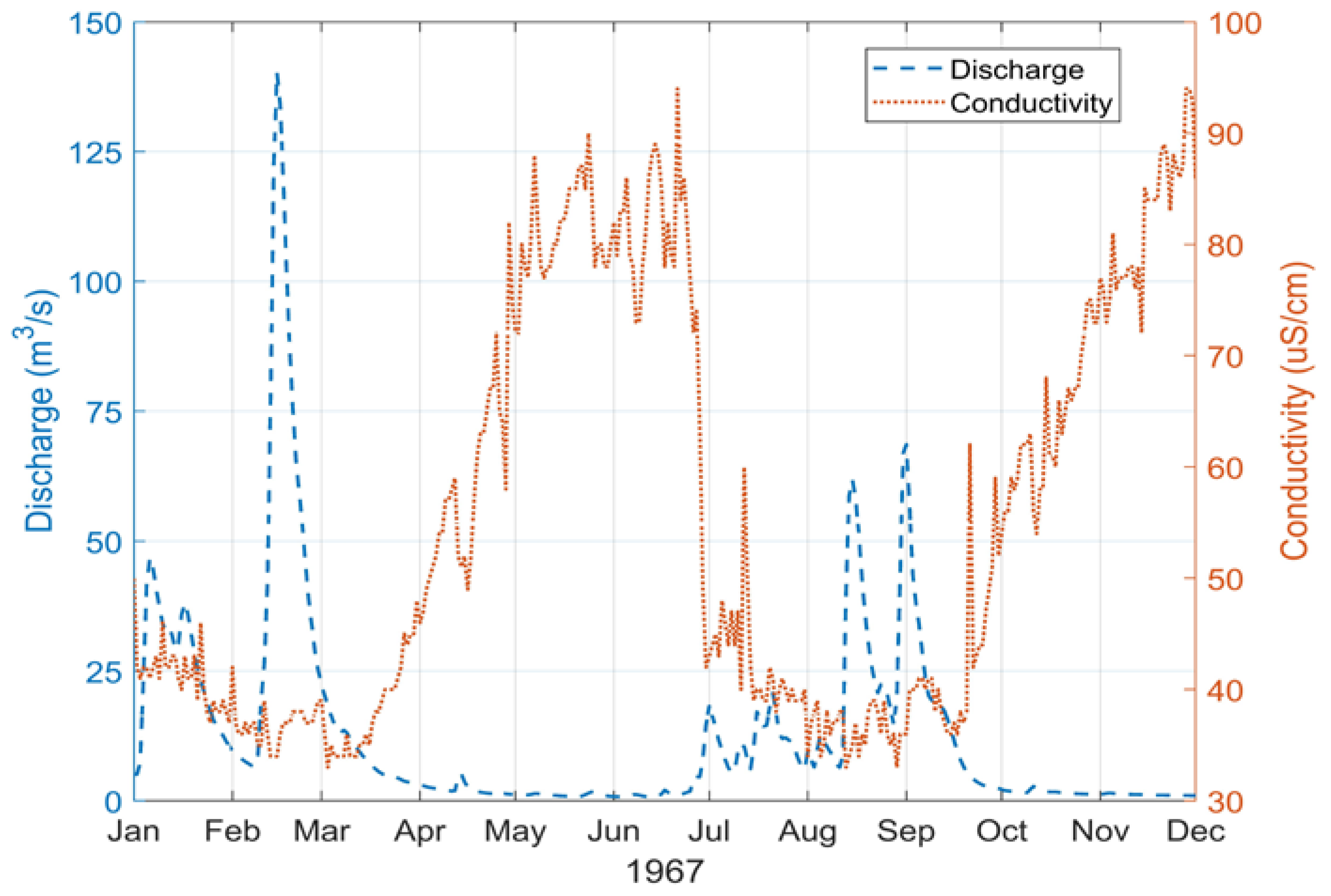
Several recent studies used different baseflow separation methods to derive the baseflow data. The HYSEP [27] program includes three approaches, which are fixed-interval, sliding-interval, and local-minimum. Several studies [5,28,29,30,31] used the HYSEP method to generate a baseflow hydrograph for a long time period. BFLOW [32] is a one parameter filter model based on signal analysis. Recently, multiple studies [17,33,34,35] used this method to estimate the baseflow value from streamflow records. The PART [36] program uses information about the antecedent streamflow recession, and it is similar to the HYSEP local-minimum method. The PART method can be used with a long time period streamflow record to estimate the mean value of baseflow. Multiple studies [8,37,38] separated the baseflows from streamflows using the PART method. The Web based Hydrograph Analysis Tool (WHAT) [39] is another one parameter digital filter method that can be used to obtain daily/monthly direct runoff and baseflow from daily/monthly streamflow records. The WHAT program runs a local-minimum, BFLOW filter method and an Eckhardt filter method to generate hydrographs for the specified period. Several studies [40,41,42,43] documented the use of the WHAT method to estimate baseflow in different watersheds. However, measurements of baseflows are difficult, expensive, and rare and are limited to small scale field studies funded under unique research experimental sites. Conductivity measurements of streams can provide beneficial information about baseflows. The conductivity mass balance (CMB) method [44] relates to concentrations of the composite chemicals in any stream. The conductivity of streamflow is normally lower than that of the baseflow, and higher discharges are linked with lower values of water conductivity, as shown in Figure 1. Multiple studies [40,44,45] used the baseflows derived from the CMB method as an acceptable and defensible substitute for measured (i.e., observed) data to calibrate and validate different methods and also compare the results from the methods.
The main objectives of this study are to: (1) evaluate baseflow values obtained from four different baseflow separation methods and baseflows from the CMB method using historical streamflow data from the period 1970–2013 in the SAG region; (2) quantify the contribution of daily baseflow values in the SAG region; (3) calibrate and validate baseflows estimated with four different methods and the CMB method; (4) assess the characteristics of the baseflow index (BFI) to identify a baseflow separation method that is most appropriate for the region.
2. Materials and Methods
According to a recent review of baseflow separation methods by Teegavarapu [46], baseflow separation methods can be classified into two major categories: (1) continuous hydrographic separation techniques and (2) graphical methods. In this study, HYSEP [27], WHAT [39], BFLOW [32], and PART [36] baseflow separation methods were evaluated at several sites in the South Atlantic-Gulf (SAG) region. The estimates of baseflows provided by the conductivity mass balance (CMB) method [44] were considered to be surrogates for the observed baseflows in this study. Brief descriptions of these methods are provided in the following sections.
2.1. HYSEP
Sloto and Crouse (1996) developed the HYSEP method to separate the baseflow and surface runoff components of daily streamflow. The HYSEP method includes three approaches: (i) fixed-interval, (ii) sliding-interval, and (iii) local-minimum. The duration of surface runoff that is required in the three methods of HYSEP is computed using Equation (1):
where the variable is the number of days after which surface runoff ceases and is the drainage area in square miles [47]. The fixed-interval method finds the lowest discharge in each interval (2*, where * is the integer). The sliding-interval method assigns the lowest discharge in one half the interval minus one day (0.5(2* − 1) days). The local-minimum method uses the same interval as the sliding interval method, and the local-minimum is used for the evaluation of baseflows in this study.
2.2. WHAT
The Web based Hydrograph Analysis Tool (WHAT) [39] is a one parameter digital filter method that can be used to obtain daily/monthly direct runoff and baseflow from daily/monthly streamflow records. WHAT uses the local-minimum, BFLOW filter method, and Eckhardt filter method to generate the hydrograph for a specified period. The WHAT method uses Equation (2) to estimate baseflow:
where is the filtered baseflow, is the maximum baseflow index, is the recession constant, is the total streamflow, and is the time interval. Eckhardt [28] recommended a value of 0.8 for perennial streams with porous aquifer conditions, 0.5 for ephemeral streams with porous aquifer conditions, and 0.25 for perennial streams with hard rock aquifer conditions. The values were suggested by Eckhardt [28] who tested and validated the WHAT method in Illinois, Pennsylvania, and Maryland.
2.3. BFLOW
BFLOW [32] is also a one parameter filter model based on signal analysis methods. A few studies used this method to estimate baseflow value from streamflow records. The baseflow in the BFLOW method is obtained using Equation (3) [48]:
where is the filtered baseflow, is the total streamflow, is the number of time steps, and is the recession constant. In Equation (3), a value of 0.925 was used for α in the BFLOW method.
2.4. PART
The PART [36] program utilizes information about the antecedent streamflow recession, and it uses a similar procedure that is employed by the HYSEP local-minimum method. The PART method can be used with a long time series of streamflows to estimate the mean value of baseflow. PART uses streamflow partitioning to estimate a daily record of groundwater discharge from daily streamflow data [36]. The program can be applied to a considerable period of record to give an estimate of the mean rate of ground water discharge or adequate recharge.
2.5. CMB Method
The conductivity mass balance (CMB) [44] method is based on a correlation of higher composite chemical concentrations with higher water conductance in a stream. In general, the baseflow conductivity value is equivalent to that of streamflow during extreme low flow periods or when the water table elevation is lower than the surface elevation. The conductivity of surface runoff value is considered to be the value of conductivity of streamflow at peaks during extreme high flow periods. The CMB method estimates baseflows based on Equation (4) [44]:
where is the total baseflow, is the total streamflow, is the conductivity of streamflow, is the conductivity of surface runoff, and is the conductivity of baseflow.
2.6. Baseflow Index
The baseflow index (BFI), which is the contribution of baseflow from streamflow throughout the record, was used to compare the analysis results of four baseflow separation methods. The BFI value is calculated using Equation (5):
where the variable is the total volume of baseflow during the period 1970–2013 and is the total volume of streamflow in the same period. The value of BFI lies between 0 and 1.
2.7. Calibration and Validation of Four Baseflow Separation Methods with the CMB Method
In the HYSEP and PART methods, the procedures to calibrate baseflows were estimated by those methods considered to use the one parameter value (2*). Minimization of the root mean squared difference (RMSD) between CMB derived baseflow values and the estimated baseflow values of HYSEP and PART. In the WHAT method, calibration was carried out by adjusting the value until the minimum RMSD between CMB baseflow values and those from the WHAT method was obtained. The value was changed to minimize the RMSD for the BFLOW method. Approximately 50% of the data was used to calibrate the models, and the rest was used for validation. The correlation coefficient () and determination coefficient () were used to assess the performances of different methods by comparing BFI values from CMB and the four methods’ BFI. The RMSD value used as an objective function in mathematical programming formulation for calibration is calculated using Equation (6) [49]:
where is baseflow estimated by the four baseflow separation methods, is the observed baseflow derived from the CMB method, and is the total number of baseflow values.
3. Study Domain and Data
The South Atlantic-Gulf watershed region, with an area around 367,740 square kilometers, is the primary watershed area in the continental United States. This hydrological region includes the following states: Florida, South Carolina, North Carolina, Alabama, Virginia, Georgia, Louisiana, Tennessee, and Mississippi. The South Atlantic-Gulf (SAG) region is classified by USGS with the hydrologic unit code (HUC) with two digits (i.e., HUC two digit). The SAG region includes 18 subregions with four digit hydrologic unit codes (i.e., HUC-4). The available streamflow gauging sites from the Hydro-Climatic Data Network (HCDN) were grouped into four sub-regions (i.e., southern, northern, western, and eastern) [50]. The SAG region and HUC-4 basins are shown in Figure 2 and are listed in Table 1.
A total of 75 streamflow gauging sites in the Hydro-Climatic Data Network (HCDN) with daily streamflow data available from 1970–2013 in the SAG region were used in this study. The HCDN includes more than 1000 sites that span across the United States, and the network provides valuable long term streamflow data [50]. Three main reasons for choosing sites from the HCDN were: (i) the datasets from HCDN were from basins that have the least anthropogenic influences (human activities, land use changes, and deforestation); (ii) the daily streamflow data values were unimpaired for less than five calendar years, so that they could be used in hydrological baseflow separation processes; (iii) the locations of the HCDN sites were close to rivers, basins, and reservoirs. A total of 11 out of 75 sites had water specific conductance data based on the evaluation of the water quantity and quality database of the USGS. These datasets were used to derive baseflows from the CMB method and to calibrate and validate four methods.
4. Results and Discussion
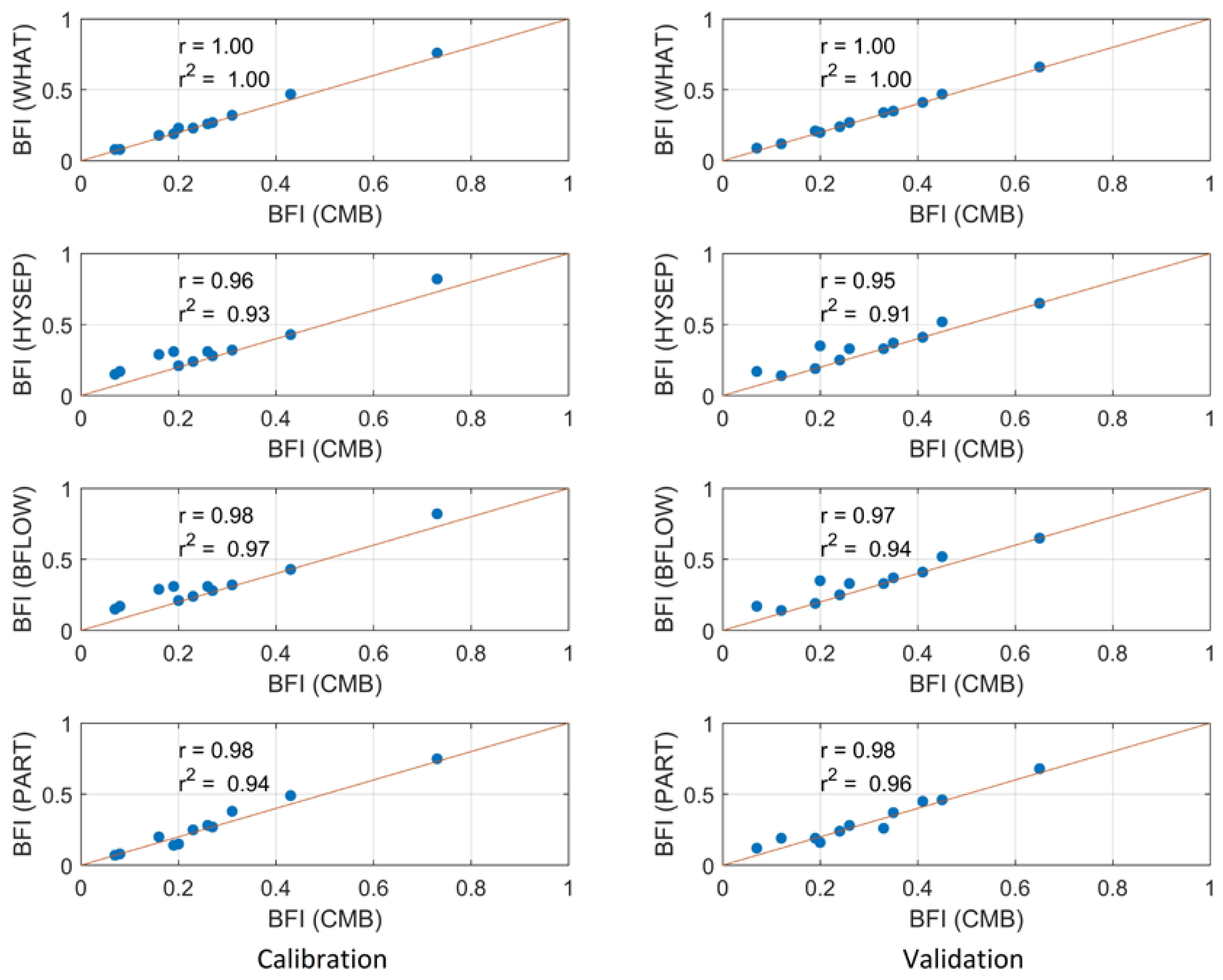
The baseflows derived by the CMB method served as a substitute for the observed baseflows. The four methods were calibrated using a nonlinear optimization model solved using a gradient based solver. For example, the calibration of baseflow values from the WHAT method by changing to minimize the value of RMSD between the CMB and WHAT methods’ baseflows. Figure 3 shows the correlation (strength of linear association) between four different baseflow methods (WHAT, HYSEP, BFLOW, and PART) and the CMB method based on calibration of the BFI values in the 11 selected SAG watershed gages. Once the WHAT, HYSEP, BFLOW, and PART methods baseflow values were calibrated by the CMB method, the BFI values of those method were highly correlated. As a result, the calibrated WHAT method had the strongest correlation (), even though the calibrated HYSEP method provided the weakest relationship (), which still presented a significant correlation. Based on these results, the calibrated WHAT method by the CMB method could be used to estimate baseflows or BFI values in the SAG region.
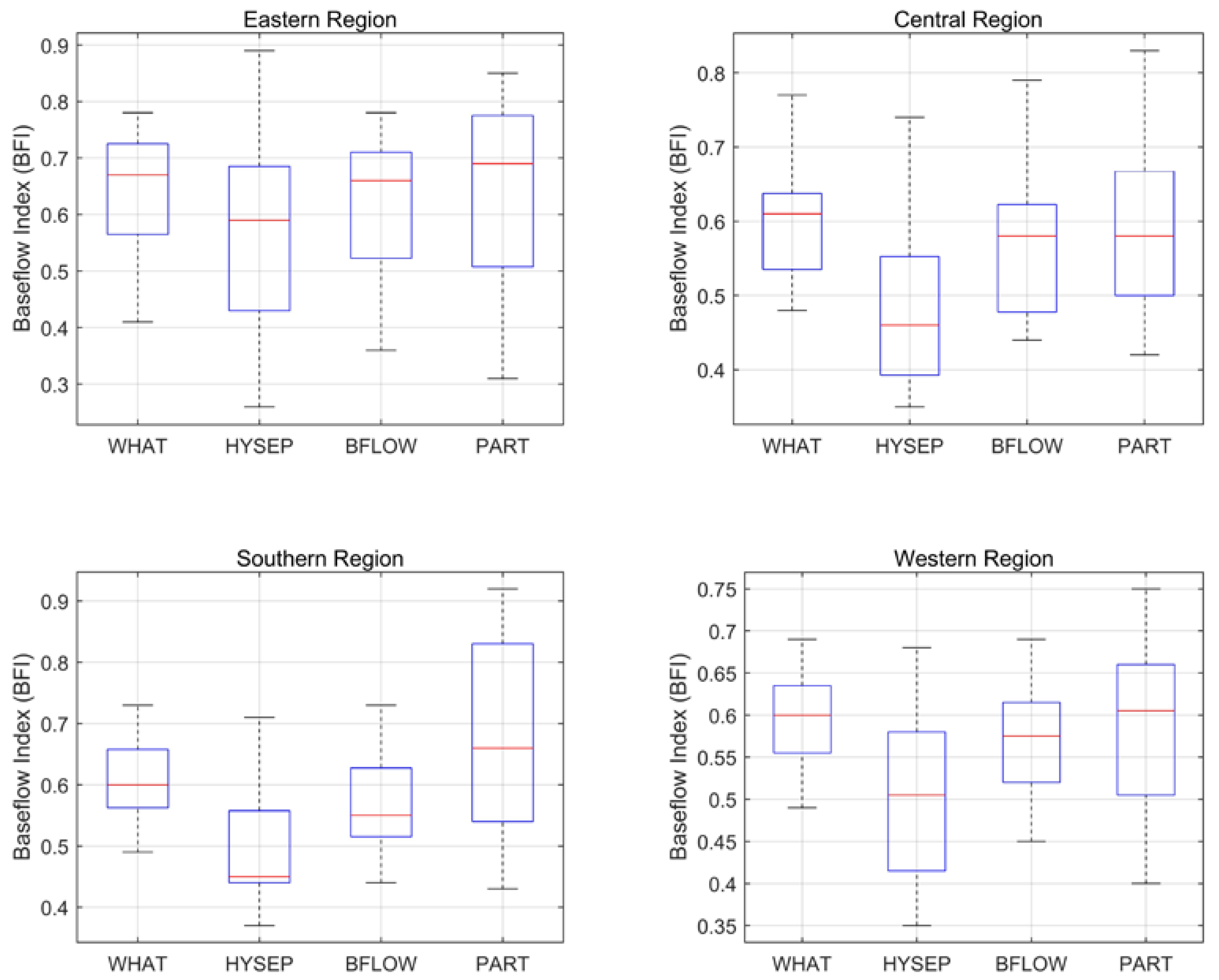
A period of record with 44 years of daily streamflow data was used to estimate baseflows in the South Atlantic-Gulf region. The range of BFI values for the WHAT method for the study region was found to be between 0.41 and 0.78, with a mean value of 0.62, and the BFI value ranges for the HYSEP, BFLOW, and PART methods were between 0.89 and 0.26, 0.79 and 0.36, and 0.92 and 0.31, with the average values of 0.52, 0.59, and 0.62, respectively. Based on the results, it could be concluded that approximately 60% of streamflow came as a baseflow contribution. The HYSEP local-minimum method provided the lowest BFI values compared to the others. According to information collected by Eckhardt [28], the maximum BFI from the WHAT method did not exceed 0.8, and the WHAT method provided a reduced number of high BFI values and an increased number of low BFI values compared to the other methods.
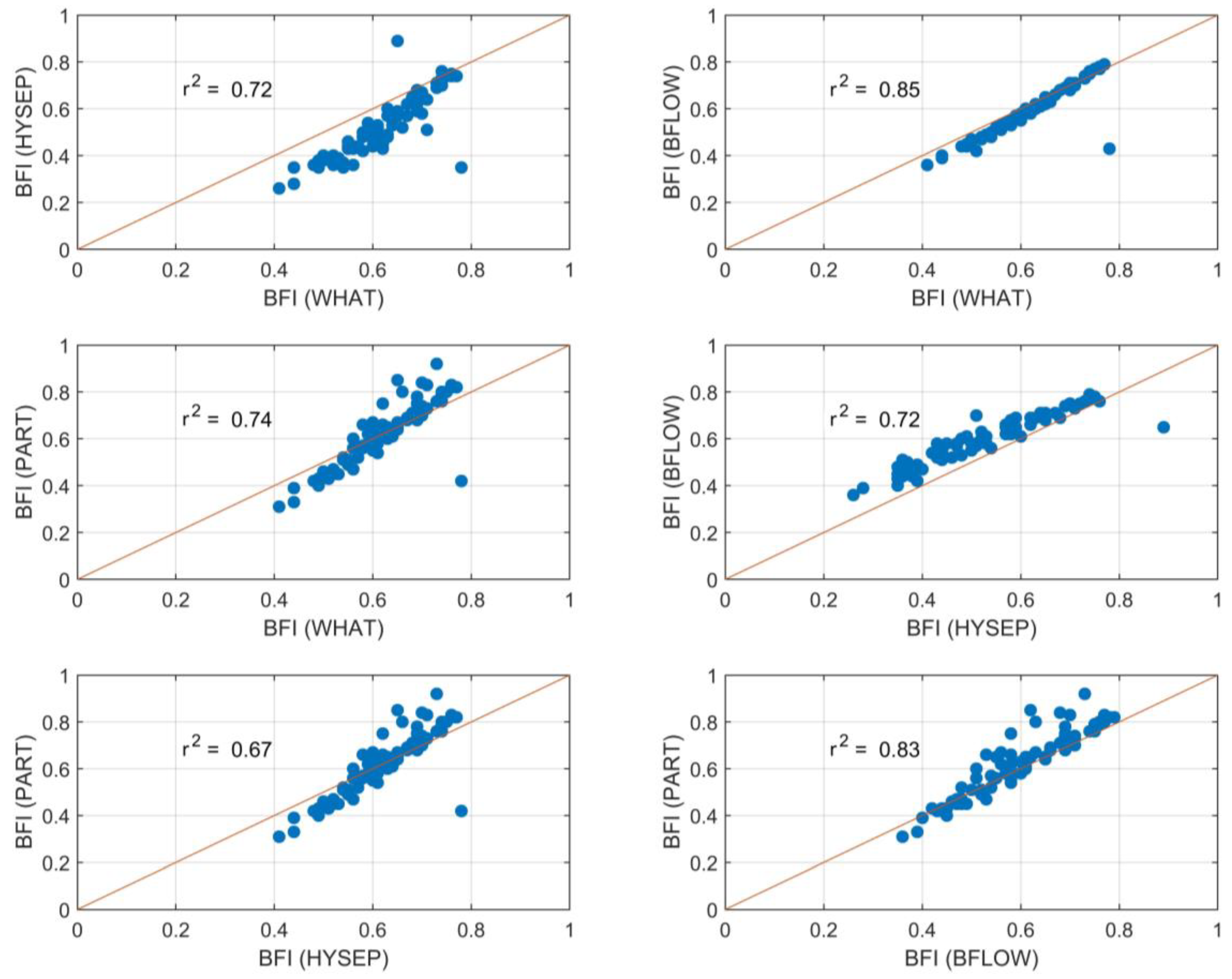
Figure 4 shows the correlation (strength of linear association) between four different baseflow methods (WHAT, HYSEP, BFLOW, and PART) based on BFI values. The figure also provides the coefficient of determination () values. It was found that the highest correlation coefficient (r) was found to be 0.92 between WHAT and BFLOW, and the lowest r value was found to be 0.82 between HYSEP and PART. Results indicated that BFI values from the WHAT method were the most similar to those from the BFLOW method. Comparisons of the baseflow index, daily mean baseflow values, daily median baseflow values, and the standard deviation of daily baseflow from the four different baseflow separation methods are shown in Figure 5. The mean of daily baseflow values for WHAT, HYSEP, BFLOW, and PART were 3.95, 3.17, 3.82, and 3.99 , respectively. It was evident that the highest average daily baseflow values were estimated by the PART method, and the lowest values were from the HYSEP local-minimum method. The BFLOW method resulted in the greatest number of outliers and higher daily baseflow medians compared to other methods.
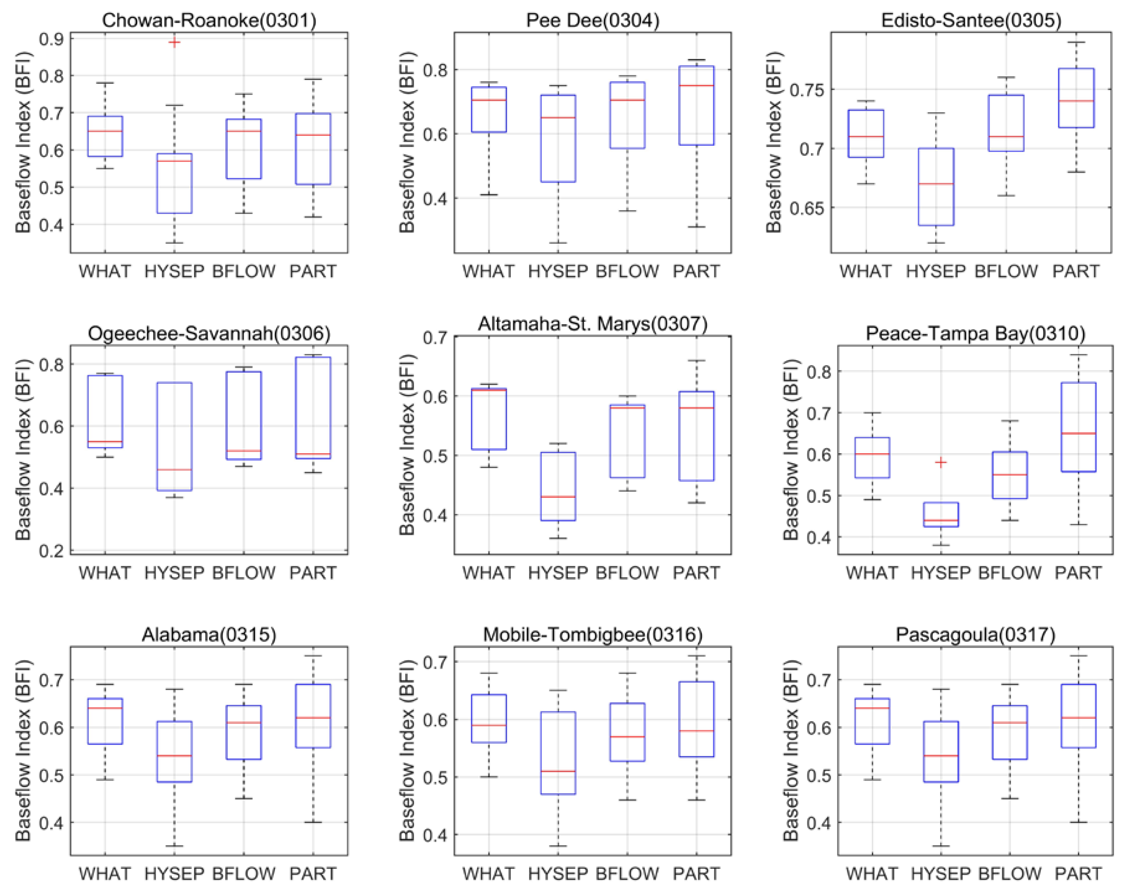
The streamflow gauging sites in the SAG region were grouped into four regions (i.e., eastern, central, southern, and western). The average of monthly baseflow values in the western region were found to be highest and lowest in the southern region during the period 1970–2013. Multiple summary statistics values (i.e., mean, median, standard deviation, skewness, and kurtosis) of the BFI values for each region using different baseflow separation methods are provided in Table 2. The comparison of the BFI values from four different baseflow separation methods in the four subregions of the SAG region is shown in Figure 6. Stations in the eastern subregion showed the largest mean and median values of BFI compared those from other subregions. It could be considered that the major portion of the streamflow came from baseflow as this flow was known to be highest in the eastern region. For each region, the WHAT method resulted in the lowest standard deviation values compared to the other three methods, and the BFI values estimated by the PART and HYSEP methods had the same standard deviation values. Figure 7 shows the comparisons of the BFI values from different baseflow separation methods in nine subregions. The Edisto-Santee subregion showed the highest BFI values, and the lowest values of BFI were found to be in the Ogeechee-Savannah subregion. A total of three (0304, 0305, and 0310) subregions displayed the highest median of the BFI values from the PART method located in the eastern and southern regions. A total of five (0306, 0307, 0315, 0316, and 0317) subregions showed the highest BFI median values computed by the WHAT method in the central and western regions.
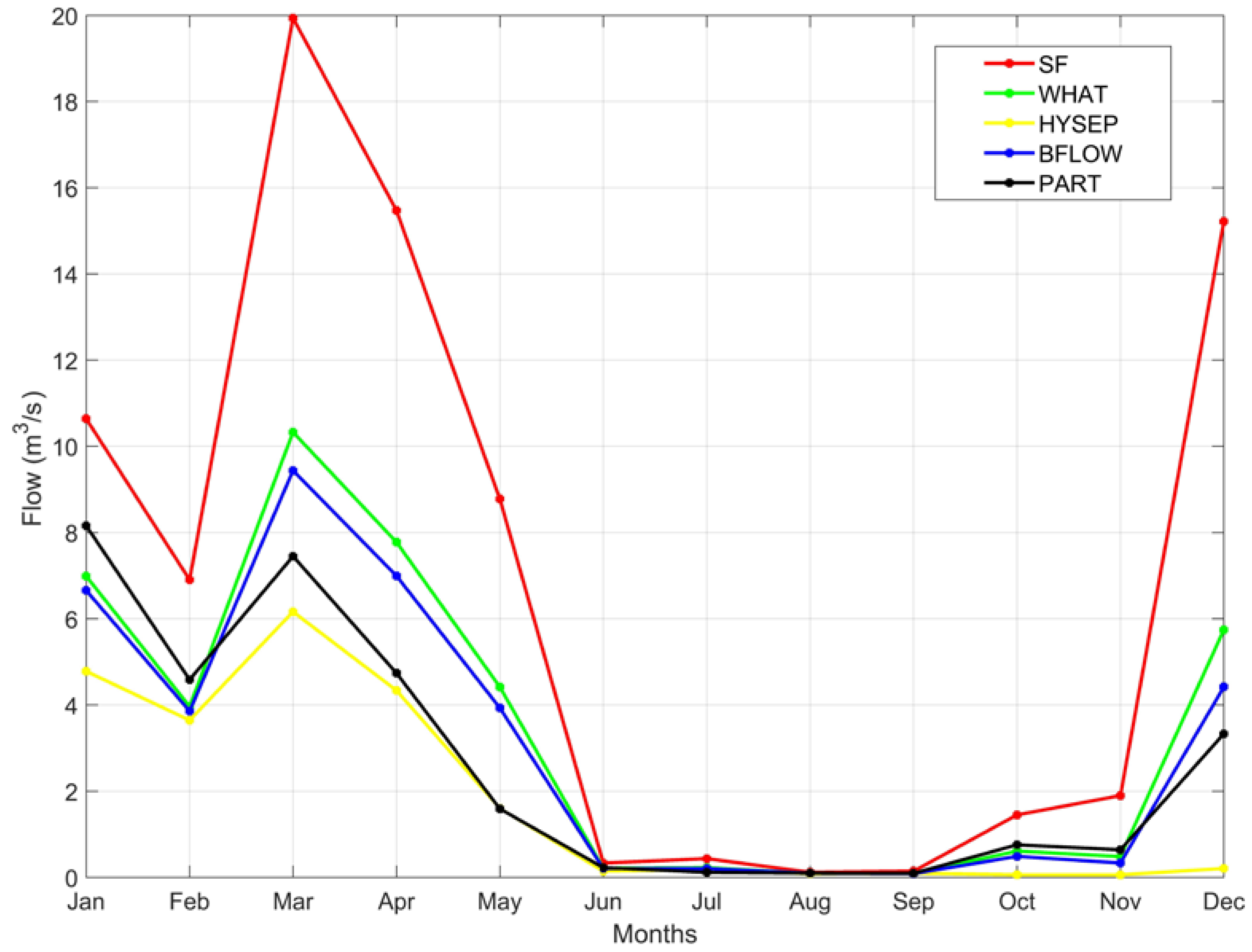
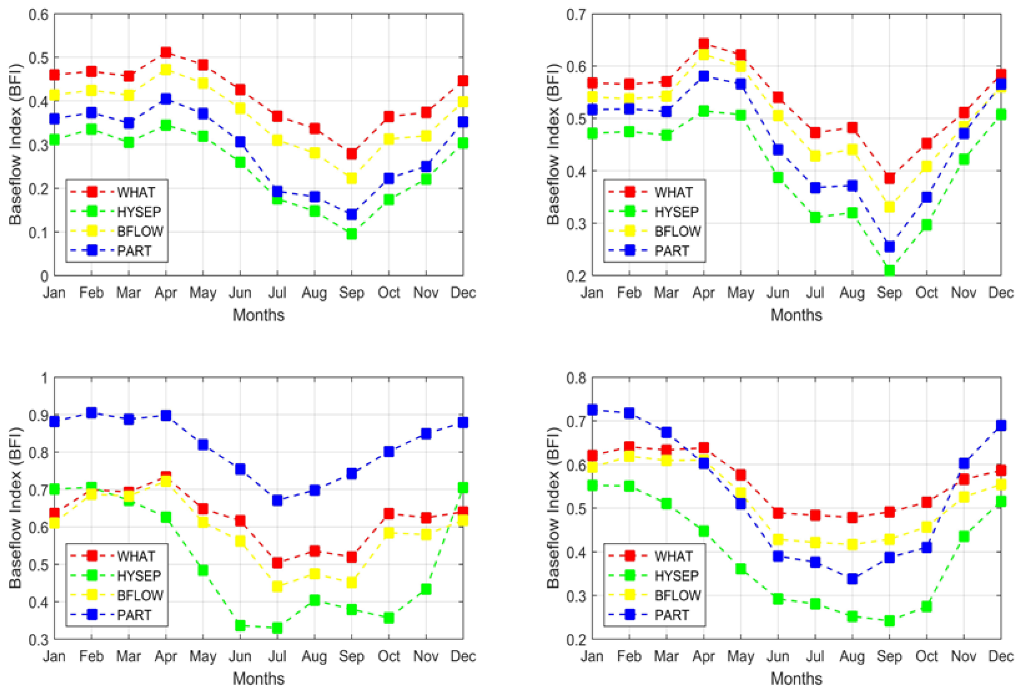
The monthly streamflows and baseflows based on the four different methods at the station of the Sopchoppy River from 1970 to 2013 are shown in Figure 8. The four different baseflow separation methods showed that values of monthly baseflows had large differences when compared to streamflow values during the months when streamflow was at peak values and minor differences in those during the months when the streamflows were the lowest. Duki et al. [35] noted a similar behavior when they reported results from the baseflow separation methods used in their study. The monthly baseflows from the HYSEP local-minimum method were slightly lower than those from others in most of the months, and baseflows estimated from the WHAT method provided the highest values. The monthly BFI curves from the four stations in the Neuse-Pamlico (0302) subregion located in the eastern SAG region are shown in Figure 9. It was evident from the BFI values that the lowest BFI values were noted from June to September and the highest values from January to April. These results suggested that the baseflow value provided less contribution to streamflow during the wet season and more during the dry season in the eastern subregion. Datta et al. [33] suggested that groundwater contributed to streamflow as high evapotranspiration losses were noted from June to September and low evapotranspiration losses from December to March and April to September in southwestern Ontario, Canada. Similar conclusions can be drawn in the current context. The BFIs had an upward trend during fall to winter and had a downward trend during spring to summer.
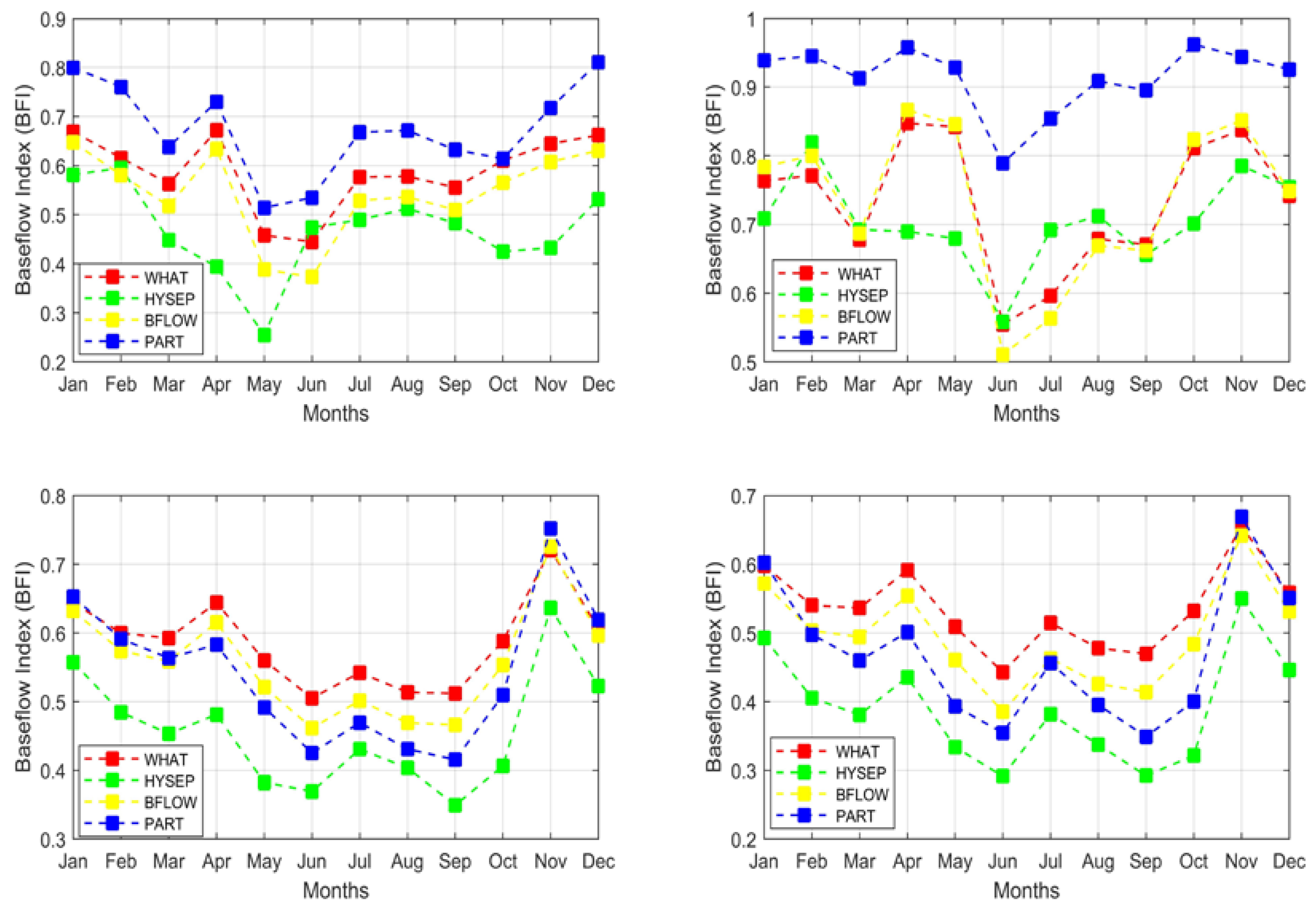
Figure 10 shows the curves of the BFI values in the Altamaha-St. Marys (0307) subregion (central area). The highest BFI appeared from August to October, and the lowest BFI values were from April to June. Bastola et al. [51] found that the minimum value of monthly average BFIs was in June, and the maximum BFIs were in October to November in the Koshi and Bagmati Basin in Nepal, which suggested the opposite to baseflow variations, as noted in the current study. The BFIs values from the four methods in the St. Johns (0308) subregion (southern area) are shown in Figure 11. The highest values of BFI were from October to November, and the lowest BFIs appeared from May to June. Notably, one of the four stations showed the lowest BFI value in September. Figure 12 shows the BFI curves from the four baseflow separation methods in the Choctawhatchee-Escambia (0314) subregion (western area). This subregion displayed different results compared to the others, and the highest BFIs occurred in September, while the lowest values immediately appeared in October. This can be attributed to regional geomorphic characteristics.
5. Conclusions
Four different baseflow separation methods (WHAT, HYSEP, BFLOW, and PART) were used to estimate and evaluate baseflow values in the South Atlantic-Gulf region in this study. As baseflow measurements (observed values) were not available in this region, conductivity mass balance (CMB) method derived estimates were considered to be substitutes for the observed baseflows. The study identified characteristics of regional baseflows and concluded that approximately 60% of streamflows were contributed by baseflows and the remaining 40% by direct runoff. The high percentage of streamflow was contributed by baseflow, which is critical information for local water resources management agencies concerned about low flows. Baseflow index (BFI) values obtained from baseflow estimates from different methods were used for comparative evaluation. BFI values from the WHAT method were the most similar to those from the BFLOW method. The calibrated WHAT method provided the best results when compared with the CMB method derived baseflow values. Therefore, the calibrated WHAT method was recommended for the estimation of baseflows or BFI values in the SAG region. Moreover, these four methods were recommended for the estimation of baseflows for the assessment of trends or changes using parametric or non-parametric statistical tests in the study area. Furthermore, the average of monthly baseflow values in the western region were highest and lowest in the southern region during the period 1970–2013, and stations in the eastern subregion showed the largest values of BFI compared to those from other subregions.
The results from this study indicated that at most of the sites, the lowest BFI values were noted from June to October and the highest values of BFI from January to April or May to June. It was also obvious that baseflows provided lower contributions to streamflows during the wet season and larger contributions to streamflows during the dry season. Assessment of the spatial variation of BFI values and baseflow characteristics in this region would aid the local water management agencies in the assessment and mitigation of regional droughts and floods. The work reported in this study can also help assess the implications of baseflow variations on low flows and water quality management strategies for the South Atlantic-Gulf (SAG) region.
Author Contributions
Conceptualization, H.C.; methodology, H.C.; validation, R.S.V.T.; formal analysis, H.C.; investigation, R.S.V.T.; writing, original draft preparation, H.C.; writing, review and editing, R.S.V.T. All authors have read and agreed to the published version of the manuscript.
Funding
This research received no external funding.
Acknowledgments
The authors sincerely thank the United States Geological Survey (USGS) for providing daily streamflow data and codes for the HYSEP and PART baseflow separation methods. We also acknowledge the help of Kyoung Jae Lim et al. for providing access to the WHAT method and Jeffrey G. Arnold and Peter Allen for providing the BFLOW method.
Conflicts of Interest
The authors declare no conflict of interest.
References
- Nerem, R.S.; Beckley, B.D.; Fasullo, J.T.; Hamlington, B.D.; Masters, D.; Mitchum, G.T. Climate-change-driven accelerated sea-level rise detected in the altimeter era. Proc. Natl. Acad. Sci. USA 2018, 115, 2022–2025. [Google Scholar] [CrossRef] [Green Version]
- Arnell, N.W.; Gosling, S.N. The impacts of climate change on river flood risk at the global scale. Clim. Chang. 2016, 134, 387–401. [Google Scholar] [CrossRef] [Green Version]
- Alfieri, L.; Feyen, L.; Dottori, F.; Bianchi, A. Ensemble flood risk assessment in Europe under high end climate scenarios. Glob. Environ. Chang. 2015, 35, 199–212. [Google Scholar] [CrossRef]
- AghaKouchak, A.; Nakhjiri, N. A near real-time satellite-based global drought climate data record. Environ. Res. Lett. 2012, 7, 044037. [Google Scholar] [CrossRef] [Green Version]
- Dai, Z.J.; Chu, A.; Du, J.Z.; Stive, M.; Hong, Y. Assessment of extreme drought and human interference on baseflow of the Yangtze River. Hydrol. Process. 2010, 24, 749–757. [Google Scholar] [CrossRef]
- Li, S.; Xiong, L.; Dong, L.; Zhang, J. Effects of the three gorges reservoir on the hydrological droughts at the downstream yichang station during 2003–2011. Hydrol. Process. 2013, 27, 3981–3993. [Google Scholar] [CrossRef]
- Abtew, W.; Trimble, P. El Niño-Southern Oscillation link to south Florida hydrology and water management applications. Water Resour. Manag. 2010, 24, 4255–4271. [Google Scholar] [CrossRef]
- Hwang, S.; Graham, W.D.; Adams, A.; Geurink, J. Assessment of the utility of dynamically-downscaled regional reanalysis data to predict streamflow in west central Florida using an integrated hydrologic model. Reg. Environ. Chang. 2013, 13, 69–80. [Google Scholar] [CrossRef]
- Patterson, L.A.; Lutz, B.; Doyle, M.W. Streamflow changes in the south Atlantic, United States during the mid- and late 20th century. J. Am. Water Resour. Assoc. 2012, 48, 1126–1138. [Google Scholar] [CrossRef]
- Dai, Z.; Amatya, D.; Sun, G.; Trettin, C.; Li, C.; Li, H. Climate variability and its impact on forest hydrology on South Carolina Coastal Plain, USA. Atmosphere 2011, 2, 330–357. [Google Scholar] [CrossRef] [Green Version]
- Loperfido, J.V.; Noe, G.B.; Jarnagin, S.T.; Hogan, D.M. Effects of distributed and centralized stormwater best management practices and land cover on urban stream hydrology at the catchment scale. J. Hydrol. 2014, 519, 2584–2595. [Google Scholar] [CrossRef]
- Conner, W.H.; Duberstein, J.A.; Day, J.W.; Hutchinson, S. Impacts of Changing Hydrology and Hurricanes on Forest Structure and Growth Along a Flooding/Elevation Gradient in a South Louisiana Forested Wetland from 1986 to 2009. Wetlands 2014, 34, 803–814. [Google Scholar] [CrossRef]
- Panagopoulos, Y.; Gassman, P.W.; Arritt, R.W.; Herzmann, D.E.; Campbell, T.D.; Valcu, A.; Jha, M.K.; Kling, C.L.; Srinivasan, R.; White, M.; et al. Impacts of climate change on hydrology, water quality and crop productivity in the Ohio-Tennessee River Basin. Int. J. Agric. Biol. Eng. 2015, 8, 36–53. [Google Scholar] [CrossRef]
- Laseter, S.H.; Ford, C.R.; Vose, J.M.; Swift, L.W. Long-term temperature and precipitation trends at the Coweeta Hydrologic Laboratory, Otto, North Carolina, USA. Hydrol. Res. 2012, 43, 890–901. [Google Scholar] [CrossRef]
- Wang, R.Y.; Kalin, L.; Kuang, W.H.; Tian, H.Q. Individual and combined effects of land use/cover and climate change on wolf bay watershed streamflow in southern Alabama. Hydrol. Process. 2014, 28, 5530–5546. [Google Scholar] [CrossRef]
- Reay, W.G.; Gallagher, D.L.; Simmons, G.M. Groundwater discharge and its impact on surface water quality in a Chesapeake Bay inlet. Water Resour. Bull. 1992, 28, 1121–1134. [Google Scholar] [CrossRef]
- Ahiablame, L.; Chaubey, I.; Engel, B.; Cherkauer, K.; Merwade, V. Estimation of annual baseflow at ungauged sites in Indiana USA. J. Hydrol. 2013, 476, 13–27. [Google Scholar] [CrossRef]
- Gebert, W.A.; Mandy, J.R.; Ellen, J.C.; Kennedy, J.L. Use of streamflow data to estimate baseflow/ground-water recharge for Wisconsin. J. Am. Water Resour. Assoc. 2007, 43, 220–236. [Google Scholar] [CrossRef]
- Santhi, C.; Allen, P.M.; Muttiah, R.S.; Arnold, J.G.; Tuppad, P. Regional estimation of base flow for the conterminous United States by hydrologic landscape regions. J. Hydrol. 2008, 351, 139–153. [Google Scholar] [CrossRef]
- Rumsey, C.A.; Miller, M.P.; Susong, D.D.; Tillman, F.D.; Anning, D.W. Regional scale estimates of baseflow and factors influencing baseflow in the Upper Colorado River Basin. J. Hydrol. Reg. Stud. 2015, 4, 91–107. [Google Scholar] [CrossRef] [Green Version]
- Zhang, Y.-K.; Schilling, K. Increasing streamflow and baseflow in Mississippi River since the 1940s: Effect of land use change. J. Hydrol. 2006, 324, 412–422. [Google Scholar] [CrossRef]
- Ficklin, D.L.; Robeson, S.M.; Knouft, J.H. Impacts of recent climate change on trends in baseflow and stormflow in United States watersheds. Geophys. Res. Lett. 2016, 43, 5079–5088. [Google Scholar] [CrossRef]
- Bosch, D.D.; Arnold, J.G.; Allen, P.G.; Lim, K.-J.; Park, Y.S. Temporal variations in baseflow for the Little River experimental watershed in South Georgia, USA. J. Hydrol. Reg. Stud. 2017, 10, 110–121. [Google Scholar] [CrossRef]
- Zhang, J.; Song, J.; Cheng, L.; Zheng, H.; Wang, Y.; Huai, B.; Sun, W.; Qi, S.; Zhao, P.; Wang, Y.; et al. Baseflow estimation for catchments in the Loess Plateau, China. J. Environ. Manag. 2019, 233, 264–270. [Google Scholar] [CrossRef]
- Buttle, J.M. Mediating stream baseflow response to climate change: The role of basin storage. Hydrol. Process. 2018, 32, 363–378. [Google Scholar] [CrossRef]
- Kahsay, K.D.; Pingale, S.M.; Hatiye, S.D. Impact of climate change on groundwater recharge and base flow in the sub-catchment of Tekeze basin, Ethiopia. Groundw. Sustain. Dev. 2018, 6, 121–133. [Google Scholar] [CrossRef]
- Sloto, R.A.; Crouse, M.Y. HYSEP: A Computer Program for Streamflow Hydrograph Separation and Analysis; U.S. Geological Survey Water-Resources Investigations Report No. 96-4040; U.S. Geological Survey: Reston, VA, USA, 1996; pp. 1–54.
- Eckhardt, K. A comparison of baseflow indices, which were calculated with seven different baseflow separation methods. J. Hydrol. 2008, 352, 168–173. [Google Scholar] [CrossRef]
- Meyer, S.C. Analysis of base flow trends in urban streams, Northeastern Illinois, USA. Hydrogeol. J. 2005, 13, 871–885. [Google Scholar] [CrossRef]
- Stadnyk, T.A.; Gibson, J.J.; Longstaffe, F.J. Basin-scale assessment of operational base flow separation methods. J. Hydrol. Eng. 2014, 20, 04014074. [Google Scholar] [CrossRef] [Green Version]
- Hodgkins, G.A.; Dudley, R.W. Historical summer base flow and stormflow trends for New England rivers. Water Resour. Res. 2011, 47. [Google Scholar] [CrossRef]
- Arnold, J.G.; Allen, P.M. Automated methods for estimating baseflow and ground water recharge from streamflow records. J. Am. Water Resour. Assoc. 1999, 35, 411–424. [Google Scholar] [CrossRef]
- Datta, A.R.; Bolisetti, T.; Balachandar, R. Automated linear and nonlinear reservoir approaches for estimating annual baseflow. J. Hydrol. Eng. 2011, 17, 554–564. [Google Scholar] [CrossRef]
- Rouhani, H.; Malekian, A. Automated methods for estimating baseflow from streamflow records in a semi arid watershed. Desert 2013, 17, 203–209. [Google Scholar] [CrossRef]
- Duki, S.R.H.; Seyedian, S.M.; Rouhani, H.; Farasati, M. Evaluation of base flow separation methods for determining water extraction (case study: Gorganroud River Basin). Water Harvest. Res. J. 2017, 2, 57–70. [Google Scholar] [CrossRef]
- Rutledge, A.T. Computer Programs for Describing the Recession of Ground-Water Discharge and for Estimating Mean Ground-Water Recharge and Discharge from Streamflow Records: Update; US Department of the Interior: Washington, DC, USA; US Geological Survey: Reston, VA, USA, 1998.
- Partington, D.; Brunner, P.; Simmons, C.T.; Werner, A.D.; Therrien, R.; Maier, H.R.; Dandy, G.C. Evaluation of outputs from automated baseflow separation methods against simulated baseflow from a physically based, surface water-groundwater flow model. J. Hydrol. 2012, 458, 28–39. [Google Scholar] [CrossRef] [Green Version]
- Villarini, G.; Jones, C.S.; Schilling, K.E. Soybean area and baseflow driving nitrate in Iowa’s Raccoon river. J. Environ. Qual. 2016, 45, 1949–1959. [Google Scholar] [CrossRef]
- Lim, K.J.; Engel, B.A.; Tang, Z.; Choi, J.; Kim, K.-S.; Muthukrishnan, S.; Tripathy, D. Automated web GIS based hydrograph analysis tool (WHAT). JAWRA J. Am. Water Resour. Assoc. 2005, 41, 1407–1416. [Google Scholar] [CrossRef]
- Lott, D.A.; Stewart, M.T. Base flow separation: A comparison of analytical and mass balance methods. J. Hydrol. 2016, 535, 525–533. [Google Scholar] [CrossRef]
- Combalicer, E.A.; Lee, S.H.; Ahn, S.; Kim, D.Y.; Im, S. Comparing groundwater recharge and base flow in the Bukmoongol small-forested watershed, Korea. J. Earth Syst. Sci. 2008, 117, 553–566. [Google Scholar] [CrossRef] [Green Version]
- Zhang, Y.; Ahiablame, L.; Engel, B.; Liu, J. Regression modeling of baseflow and baseflow index for Michigan USA. Water 2013, 5, 1797–1815. [Google Scholar] [CrossRef] [Green Version]
- Zomlot, Z.; Verbeiren, B.; Huysmans, M.; Batelaan, O. Spatial distribution of groundwater recharge and base flow: Assessment of controlling factors. J. Hydrol. 2015, 4, 349–368. [Google Scholar] [CrossRef] [Green Version]
- Stewart, M.; Cimino, J.; Ross, M. Calibration of Base Flow Separation Methods with Streamflow Conductivity. Ground Water 2007, 45, 17–27. [Google Scholar] [CrossRef]
- Zhang, R.; Li, Q.; Chow, T.L.; Li, S.; Danielescu, S. Base-flow separation in a small watershed in New Brunswick, Canada, using a recursive digital filter calibrated with the conductivity mass balance method. Hydrol. Process. 2013, 27, 2659–2665. [Google Scholar] [CrossRef]
- Teegavarapu, R.S.V. Floods in Changing Climate; Cambridge University Press: New York, NY, USA, 2012. [Google Scholar]
- Lnsley, R.K.J.; Kohler, M.A.; Paulhus, J.L.H. Hydrology for Engineers, 3rd ed.; McGraw-Hill: New York, NY, USA, 1982; p. 237. [Google Scholar]
- Lyne, V.D.; Hollick, M. Stochastic Time-Variable Rainfall-Runoff Modeling. In Proceedings of the Hydrology and Water Resources, Symposium Institution of Engineers Australia, Perth, Australia, 10–12 September 1979; pp. 89–92. [Google Scholar]
- Lee, J.; Kim, J.; Jang, W.S.; Lim, K.J.; Engel, B.A. Assessment of baseflow estimates considering recession characteristics in SWAT. Water 2018, 10, 371. [Google Scholar] [CrossRef] [Green Version]
- Slack, J.R.; Landwehr, J.M. Hydro-Climatic Data Network (HCDN): A U.S. Geological Survey Streamflow Data Set of the United States for the Study of Climate Variations,1874–1988; USGS Open-File Report 92-129; U.S. Geological Survey (USGS): Reston, VA, USA, 1992; p. 193.
- Bastola, S.; Seong, Y.; Lee, D.; Youn, I.; Oh, S.; Jung, Y.; Choi, G.; Jang, D. Contribution of baseflow to river streamflow: Study on Nepal’s Bagmati and Koshi basins. KSCE J. Civ. Eng. 2018, 22, 4710–4718. [Google Scholar] [CrossRef]
Figure 1.
Daily discharge and water conductivity in USGS Gauge 2,231,000, St. Marys River, near Macclenny, Florida.
Figure 1.
Daily discharge and water conductivity in USGS Gauge 2,231,000, St. Marys River, near Macclenny, Florida.

Figure 2.
Geographical location of the streamflow gauge sites in the South Atlantic-Gulf region. HUC, hydrologic unit code.
Figure 2.
Geographical location of the streamflow gauge sites in the South Atlantic-Gulf region. HUC, hydrologic unit code.

Figure 3.
Calibration and validation of pair-wise comparisons of the baseflow index (BFI) values based on four different baseflow separation methods and the conductivity mass balance (CMB) method.
Figure 3.
Calibration and validation of pair-wise comparisons of the baseflow index (BFI) values based on four different baseflow separation methods and the conductivity mass balance (CMB) method.

Figure 4.
Pair-wise comparison of the baseflow index (BFI) values from the four different baseflow separation methods.
Figure 4.
Pair-wise comparison of the baseflow index (BFI) values from the four different baseflow separation methods.

Figure 5.
BFI, mean, median, and standard deviation of daily baseflow from the four different baseflow separation methods.
Figure 5.
BFI, mean, median, and standard deviation of daily baseflow from the four different baseflow separation methods.

Figure 6.
Comparison of BFI values from four different baseflow separation methods in the eastern, central, southern, and western parts of the South Atlantic-Gulf region.
Figure 6.
Comparison of BFI values from four different baseflow separation methods in the eastern, central, southern, and western parts of the South Atlantic-Gulf region.

Figure 7.
Comparison of BFI values from four different baseflow separation methods in nine subregions of the South Atlantic-Gulf (SAG) region.
Figure 7.
Comparison of BFI values from four different baseflow separation methods in nine subregions of the South Atlantic-Gulf (SAG) region.

Figure 8.
Monthly streamflow and baseflow values of four baseflow separation methods for a site of the Sopchoppy River.
Figure 8.
Monthly streamflow and baseflow values of four baseflow separation methods for a site of the Sopchoppy River.

Figure 9.
Monthly BFI values using the four different baseflow separation methods in the Neuse-Pamlico sub-region (0302).
Figure 9.
Monthly BFI values using the four different baseflow separation methods in the Neuse-Pamlico sub-region (0302).

Figure 10.
Monthly BFI values using the four different baseflow separation methods in the Altamaha-St. Mary’s sub-region (0307).
Figure 10.
Monthly BFI values using the four different baseflow separation methods in the Altamaha-St. Mary’s sub-region (0307).

Figure 11.
Monthly BFI values using the four different baseflow separation methods in the St. Johns sub-region (0308).
Figure 11.
Monthly BFI values using the four different baseflow separation methods in the St. Johns sub-region (0308).

Figure 12.
Monthly BFI values using the four different baseflow separation methods in the Choctawhatchee-Escambia sub-region (0314).
Figure 12.
Monthly BFI values using the four different baseflow separation methods in the Choctawhatchee-Escambia sub-region (0314).


Table 1.
List of sub-regions along with the details of the HUC 4 digit basins in the SAG region.
| HUC 4 Number | Sub-Region Name | Location State(s) | |
|---|---|---|---|
| 0301 | Chowan-Roanoke | Virginia and North Carolina | 49,370 |
| 0302 | Neuse-Pamlico | North Carolina | 37,050 |
| 0303 | Cape Fear | North Carolina | 23,890 |
| 0304 | Pee Dee | North Carolina, South Carolina, and Virginia | 48,860 |
| 0305 | Edisto-Santee | Georgia, North Carolina, and South Carolina | 61,790 |
| 0306 | Ogeechee-Savannah | Georgia, North Carolina, and South Carolina | 43,840 |
| 0307 | Altamaha-St. Marys | Florida and Georgia | 53,830 |
| 0308 | St. Johns | Florida | 29,490 |
| 0309 | Southern Florida | Florida | 46,110 |
| 0310 | Peace-Tampa | Florida | 25,250 |
| 0311 | Suwannee | Florida and Georgia | 35,000 |
| 0312 | Ochlockonee | Florida and Georgia | 9490 |
| 0313 | Apalachicola | Alabama, Florida, and Georgia | 52,720 |
| 0314 | Choctawhatchee-Escambia | Alabama and Florida | 38,700 |
| 0315 | Alabama | Alabama, Georgia, and Tennessee | 58,890 |
| 0316 | Mobile-Tombigbee | Alabama and Mississippi | 56,550 |
| 0317 | Pascagoula | Alabama and Mississippi | 30,990 |
| 0318 | Peart | Louisiana and Mississippi | 22,500 |
Table 2.
Summary statistics of BFI values for each region using different baseflow separation methods.
Table 2.
Summary statistics of BFI values for each region using different baseflow separation methods.
| Baseflow | Method | Eastern | Central | Southern | Western |
|---|---|---|---|---|---|
| Mean Value | WHAT | 0.65 | 0.60 | 0.61 | 0.60 |
| HYSEP | 0.56 | 0.49 | 0.49 | 0.50 | |
| BFLOW | 0.62 | 0.57 | 0.57 | 0.57 | |
| PART | 0.64 | 0.59 | 0.68 | 0.58 | |
| Median Value | WHAT | 0.67 | 0.61 | 0.60 | 0.60 |
| HYSEP | 0.59 | 0.46 | 0.45 | 0.51 | |
| BFLOW | 0.66 | 0.58 | 0.55 | 0.58 | |
| PART | 0.69 | 0.58 | 0.66 | 0.61 | |
| Standard Deviation | WHAT | 0.10 | 0.06 | 0.05 | 0.06 |
| HYSEP | 0.16 | 0.11 | 0.08 | 0.10 | |
| BFLOW | 0.13 | 0.09 | 0.06 | 0.08 | |
| PART | 0.16 | 0.11 | 0.08 | 0.10 | |
| Skewness | WHAT | −0.95 | 0.73 | 0.13 | −0.38 |
| HYSEP | −0.17 | 0.93 | 1.07 | 0.08 | |
| BFLOW | −0.73 | 0.85 | 0.40 | −0.19 | |
| PART | −0.71 | 0.72 | −0.18 | −0.35 | |
| Kurtosis | WHAT | 0.05 | −0.36 | −0.63 | −0.71 |
| HYSEP | −0.72 | −0.20 | 1.12 | −0.91 | |
| BFLOW | −0.67 | −0.28 | −0.38 | −0.71 | |
| PART | −0.64 | −0.33 | −1.27 | −0.80 |
© 2019 by the authors. Licensee MDPI, Basel, Switzerland. This article is an open access article distributed under the terms and conditions of the Creative Commons Attribution (CC BY) license (http://creativecommons.org/licenses/by/4.0/).
Share and Cite
MDPI and ACS Style
Chen, H.; Teegavarapu, R.S.V. Comparative Analysis of Four Baseflow Separation Methods in the South Atlantic-Gulf Region of the U.S. Water 2020, 12, 120. https://doi.org/10.3390/w12010120
AMA Style
Chen H, Teegavarapu RSV. Comparative Analysis of Four Baseflow Separation Methods in the South Atlantic-Gulf Region of the U.S. Water. 2020; 12(1):120. https://doi.org/10.3390/w12010120
Chicago/Turabian StyleChen, Hao, and Ramesh S. V. Teegavarapu. 2020. "Comparative Analysis of Four Baseflow Separation Methods in the South Atlantic-Gulf Region of the U.S." Water 12, no. 1: 120. https://doi.org/10.3390/w12010120
Note that from the first issue of 2016, this journal uses article numbers instead of page numbers. See further details here.