Effects of Surface Heterogeneity Due to Drip Irrigation on Scintillometer Estimates of Sensible, Latent Heat Fluxes and Evapotranspiration over Vineyards


 ,
,
Abstract
:1. Introduction
2. Data
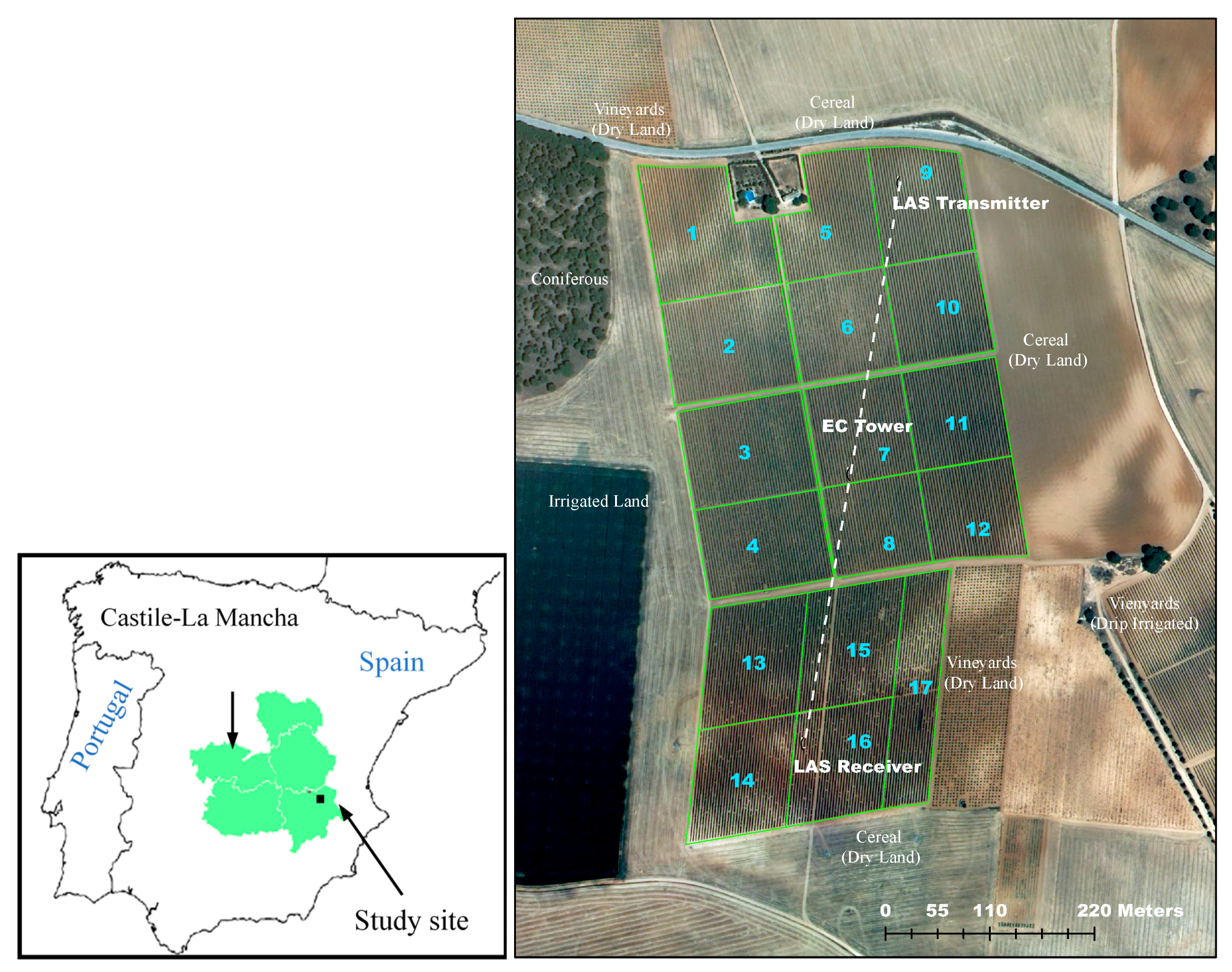
2.1. Study Area
2.2. LAS Measurements
2.3. EC Measurements
Surface Energy Balance Lack of Closure
2.4. Remote Sensing Data
2.4.1. Landsat Images
2.4.2. MODIS Images
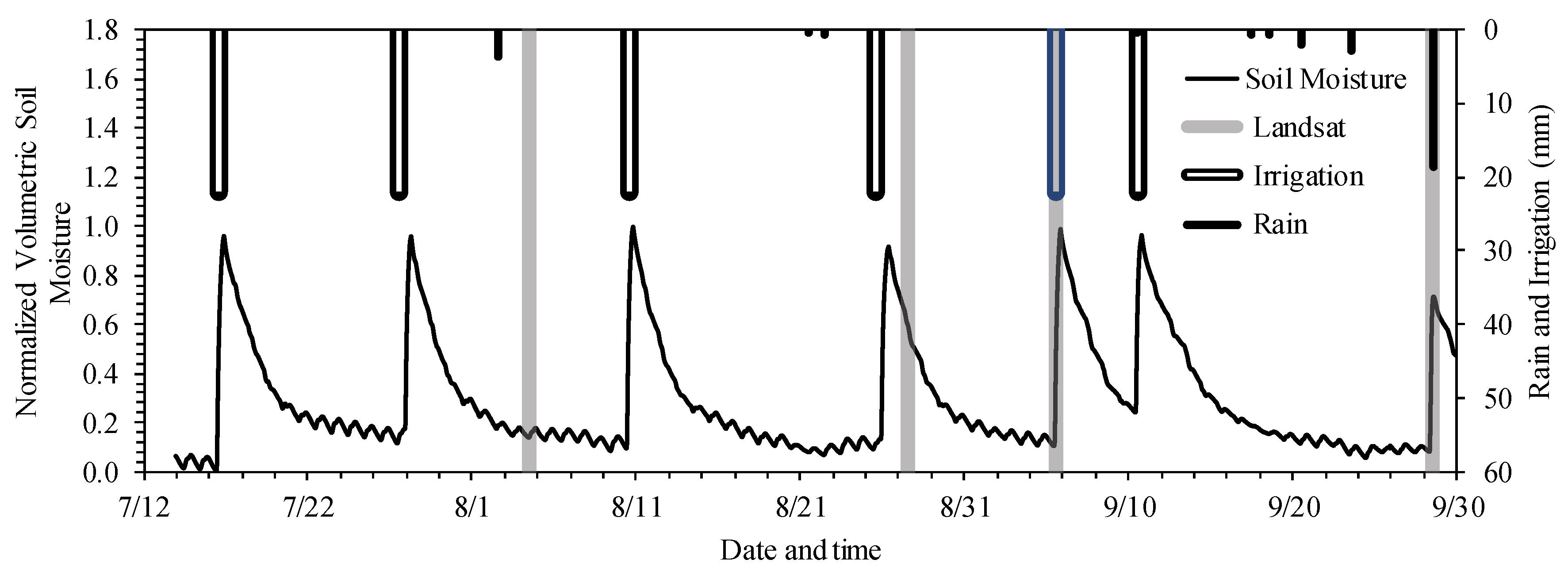
2.5. Root Zone Soil Moisture Content
3. Methods
3.1. Estimates of H Using LAS
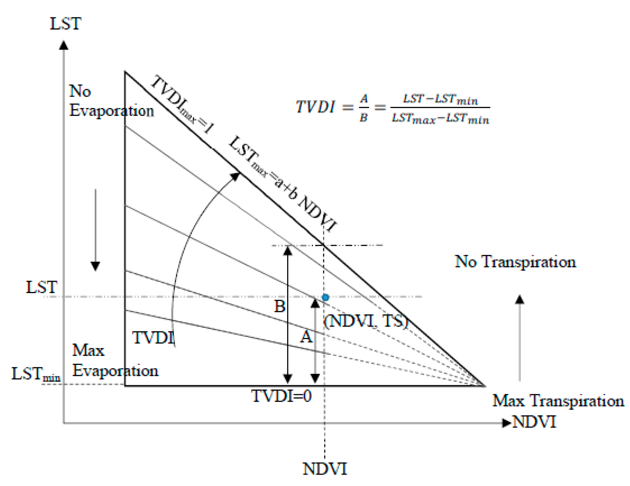
3.2. LST–NDVI Space, TVDI, and Spatial Heterogeneity
3.3. Data Fusion
3.4. The TSEB Model
3.5. Footprint Model
4. Results
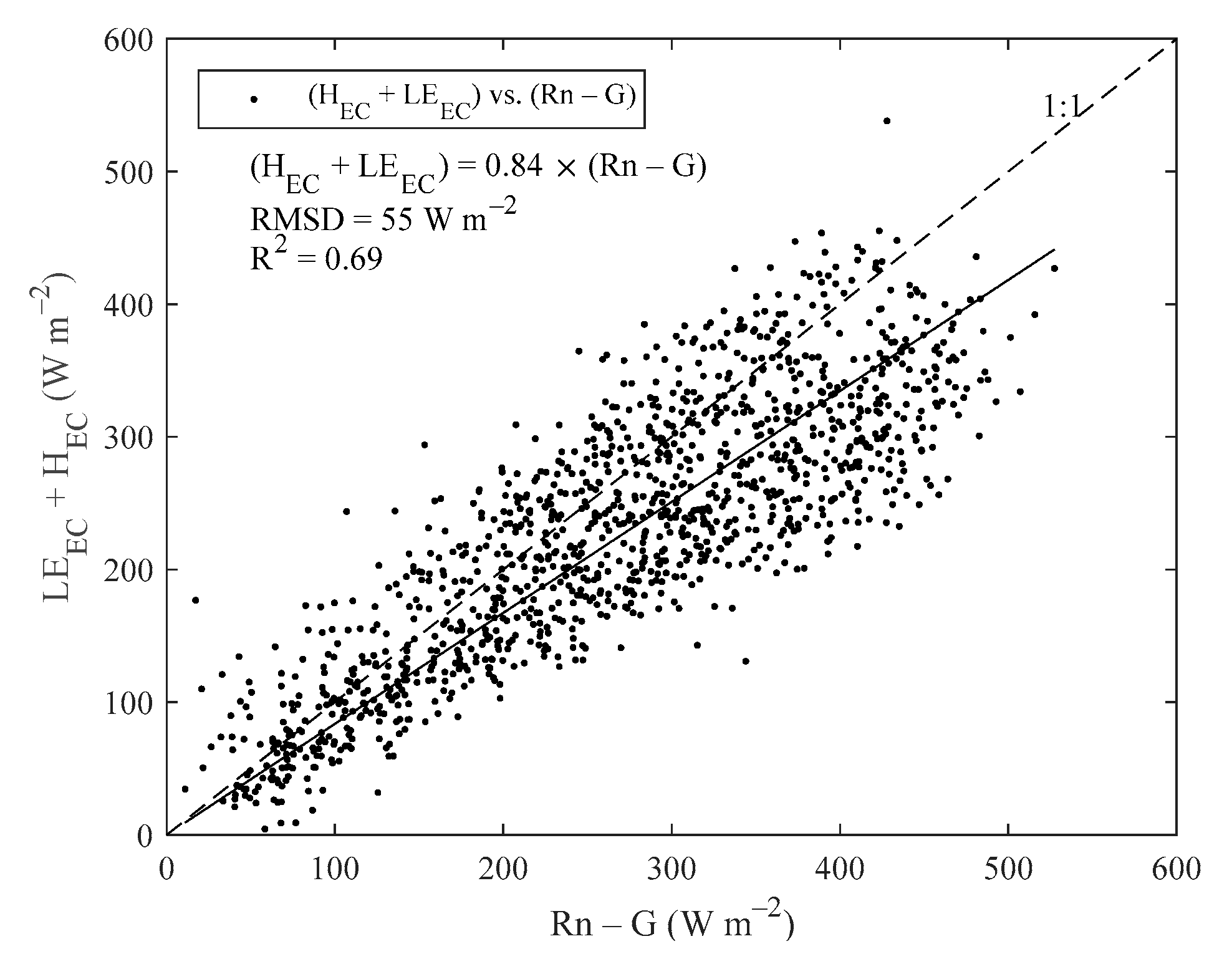
4.1. Observed Surface Energy Balance Closure
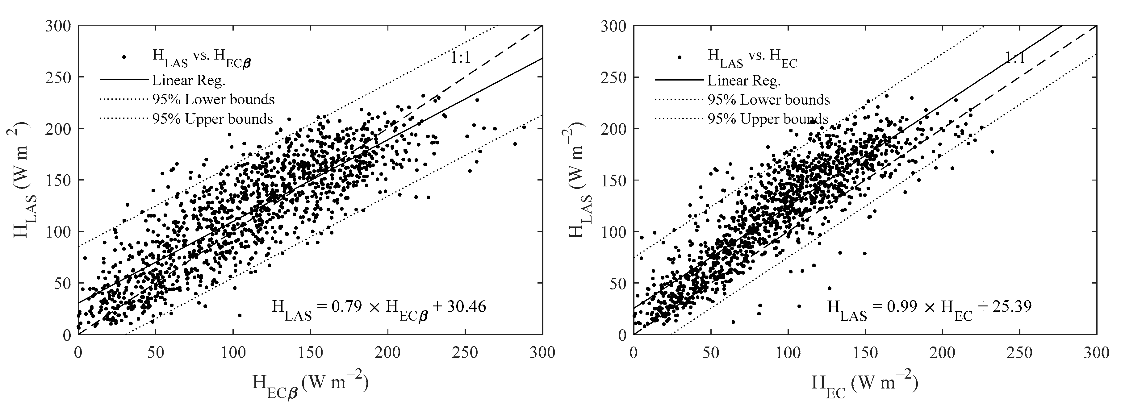
4.2. Comparison between HLAS and HEC
4.3. HLAS, Soil Moisture, and Vegetation Spatial Variability
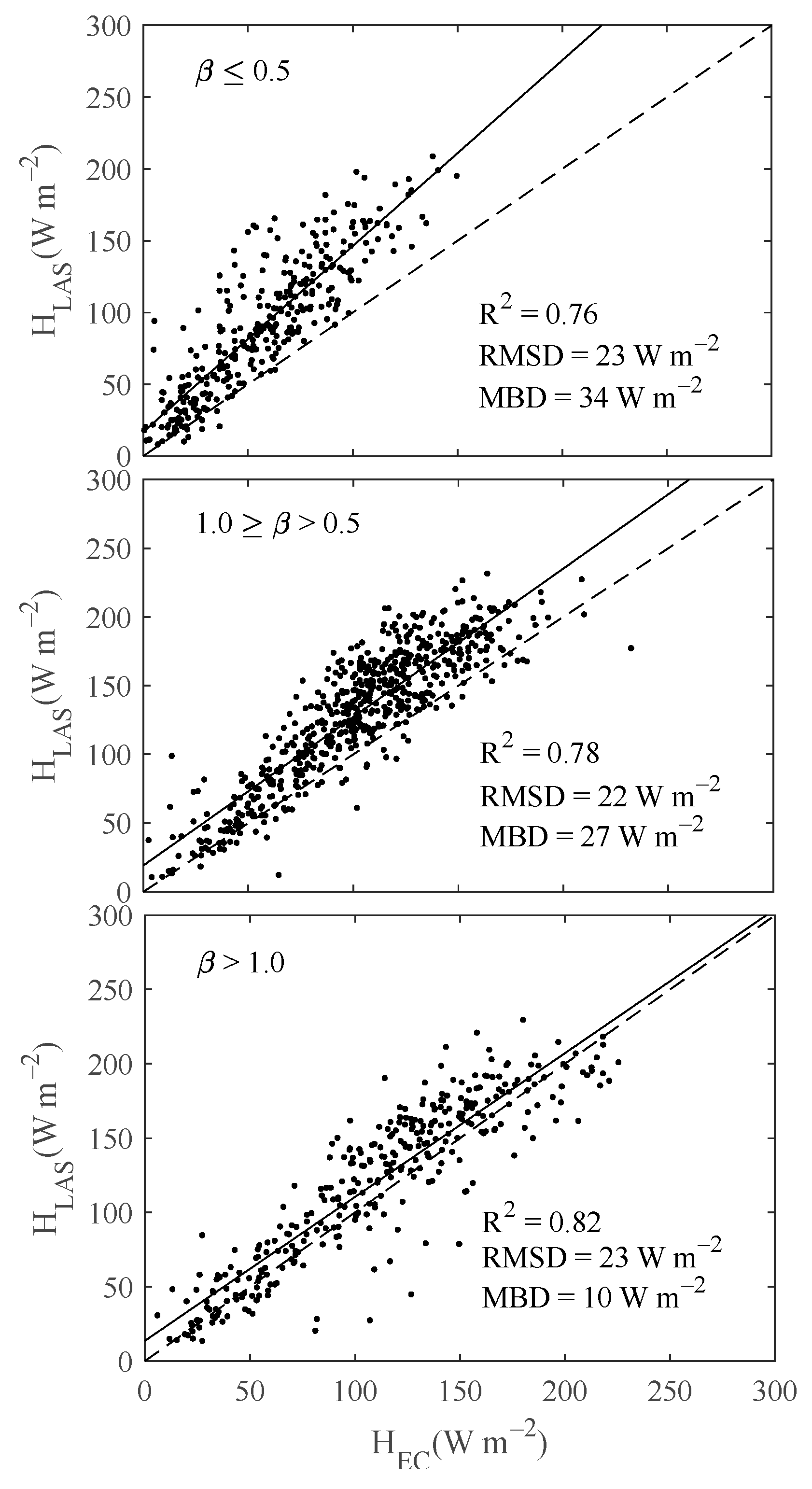
4.3.1. HLAS and β
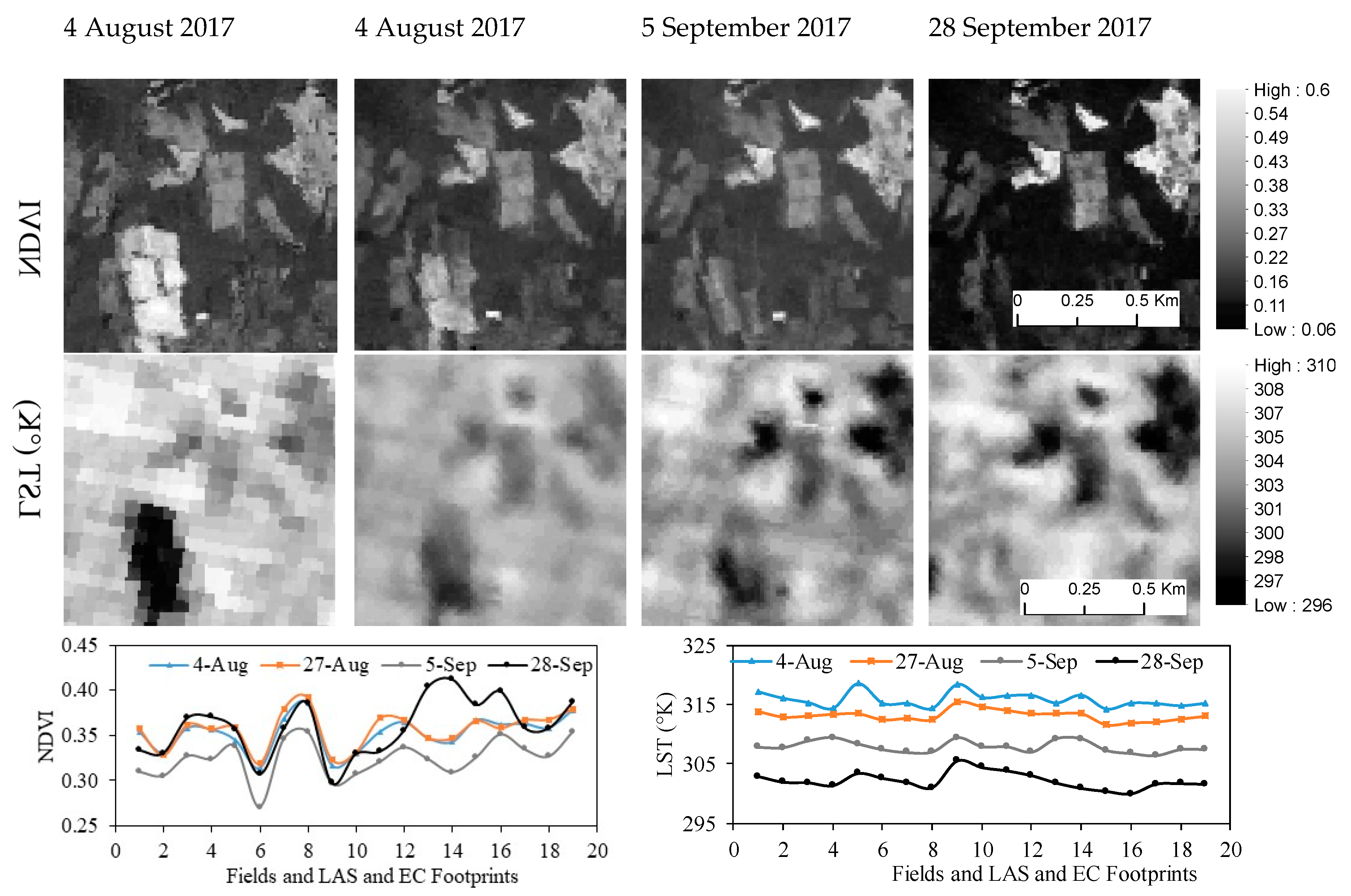
4.3.2. LST–NDVI Space and Spatial Heterogeneity
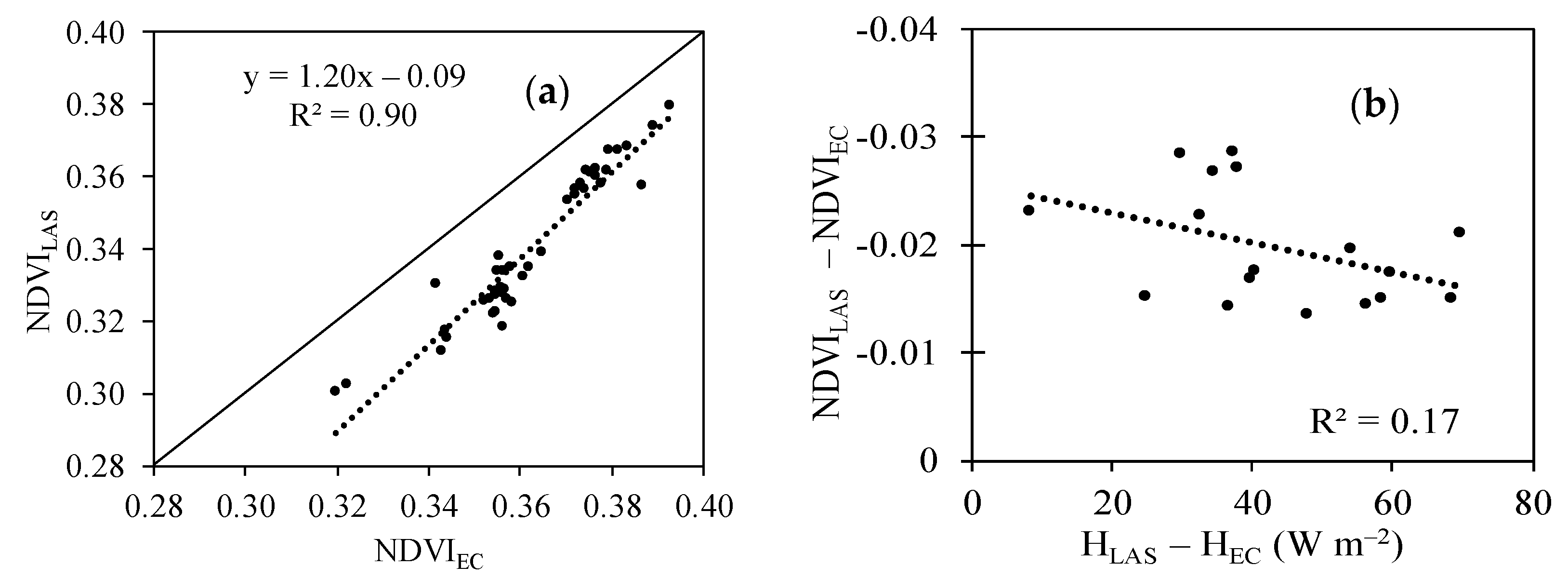
NDVI Variability
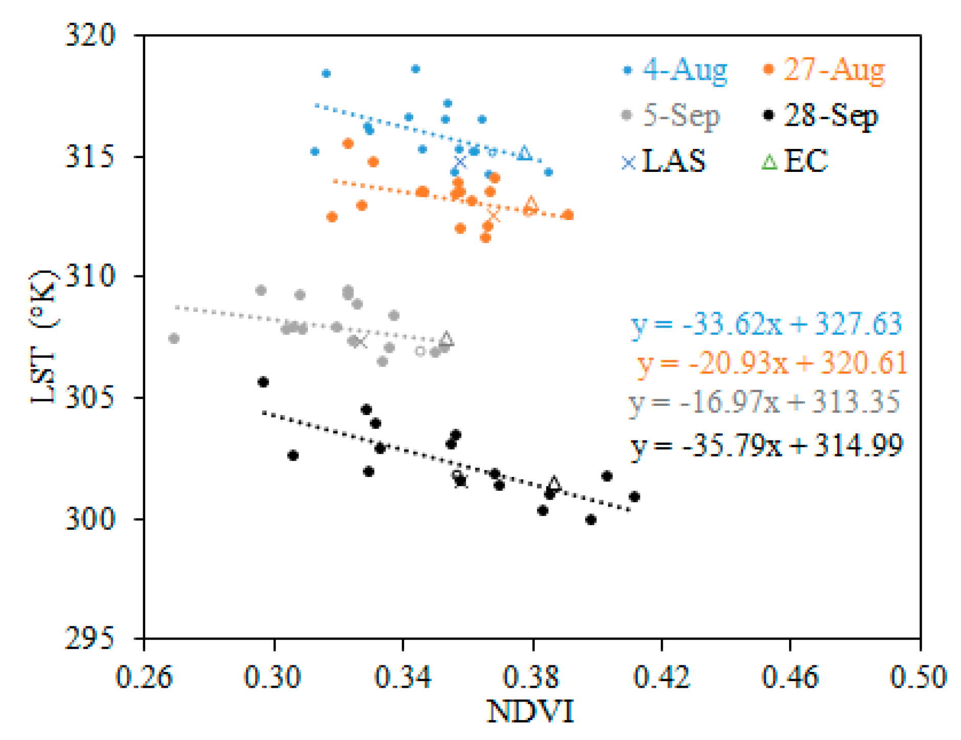
LST–NDVI Space
4.3.3. HLAS and TVDI
Estimates of TVDI
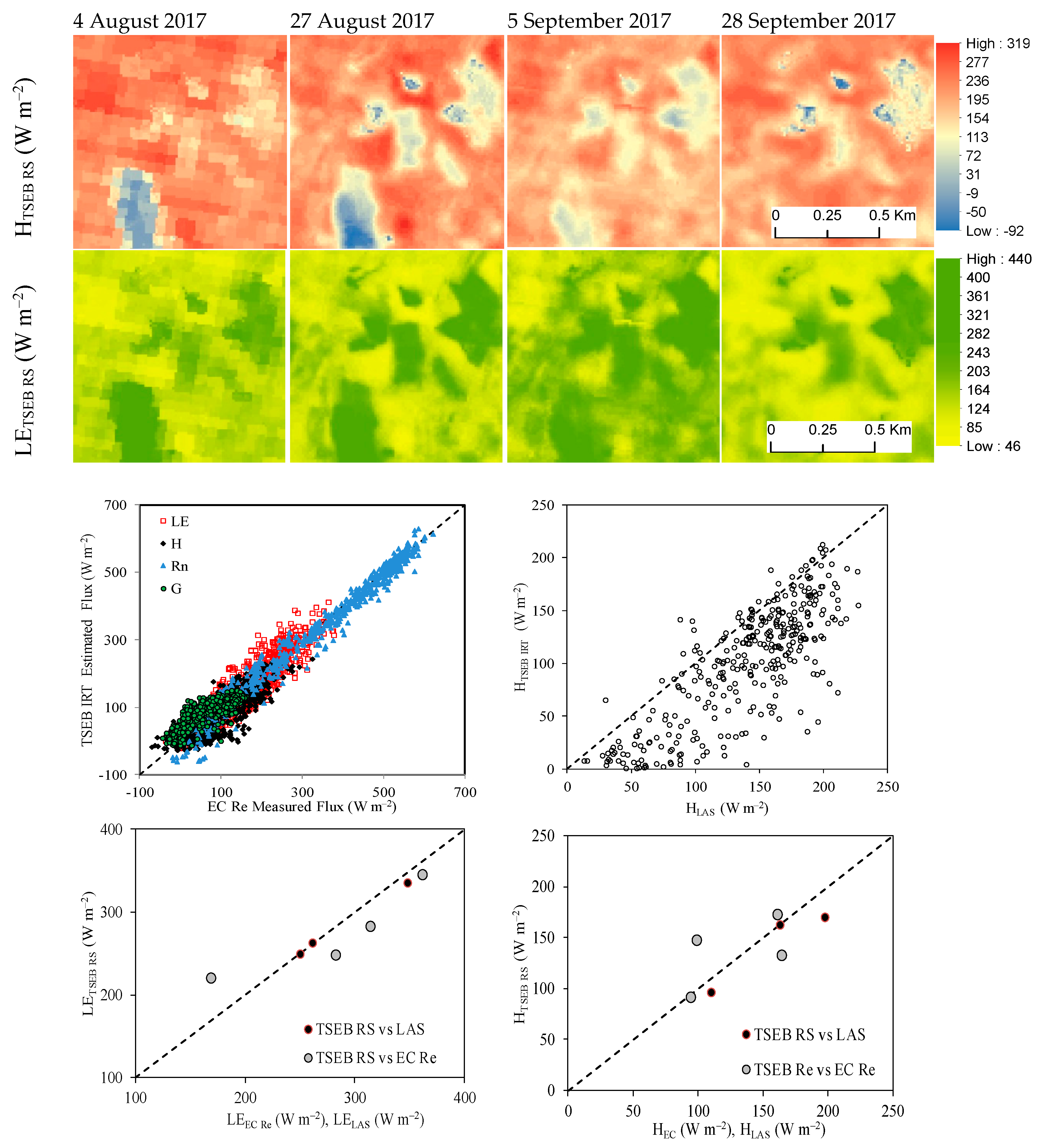
Estimates of HTSEB
HLAS and TVDI
4.4. Estimates of LE and ET
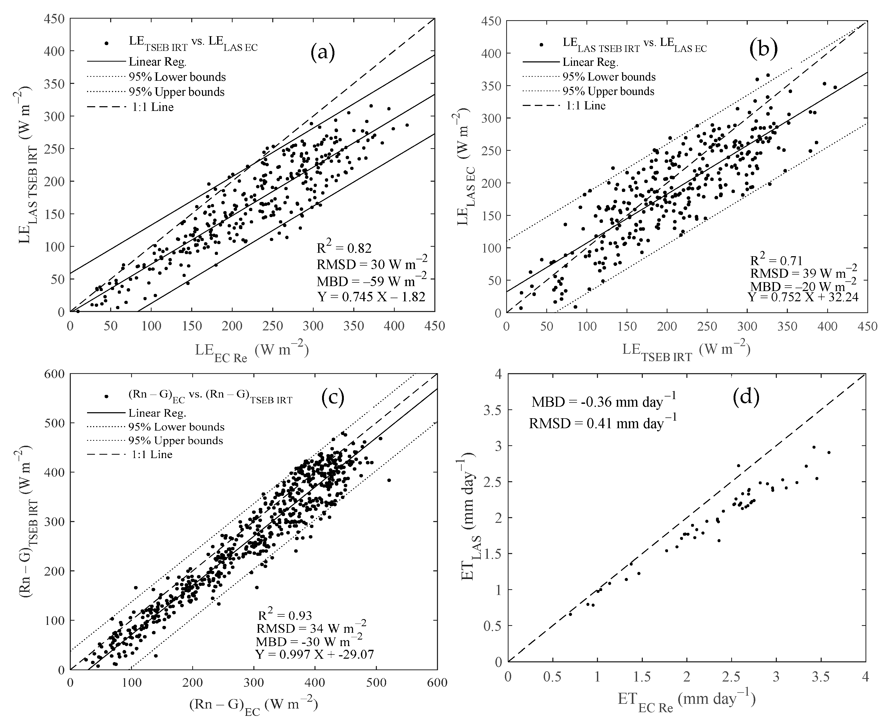
4.4.1. Estimates of LELAS
4.4.2. LELAS and TVDI
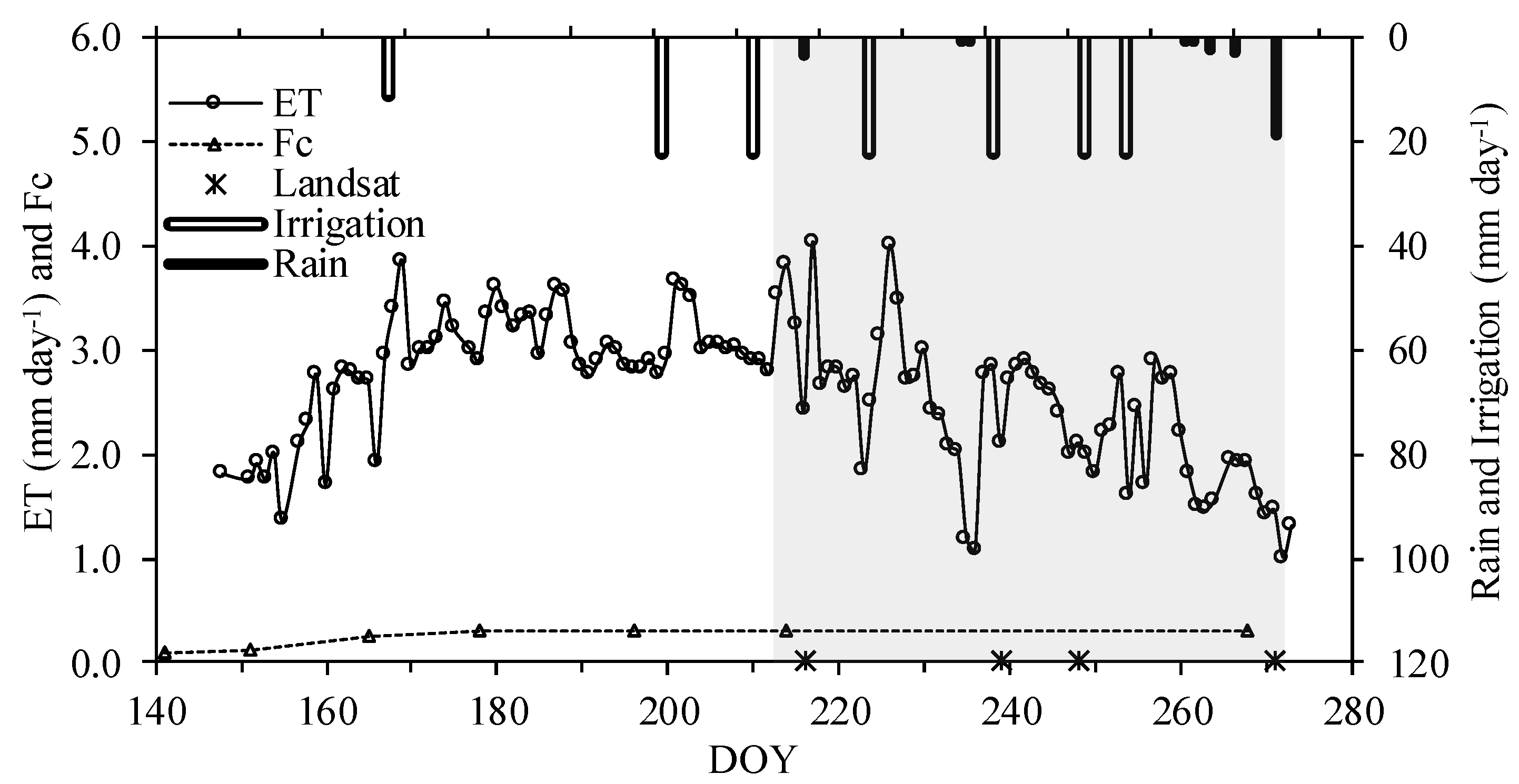
4.4.3. Estimates of ET
5. Discussion
5.1. Lack of Closure
5.2. HLAS and HEC
5.3. HLAS and β
5.4. NDVI Variability
5.5. LST–NDVI Space and Soil Moisture
5.6. HLAS and TVDI
5.7. Estimates of LELAS and ET
6. Conclusions
Author Contributions
Funding
Acknowledgments
Conflicts of Interest
Appendix A


Appendix B
Appendix B.1. Estimation of as a Function of
Appendix C
Appendix C.1. TSEB Model Description
Appendix D
Appendix D.1. Footprint Analysis
References
- Black, M. The Atlas of Water: Mapping the World’s Most Critical Resource, 3rd ed.; University of California Press: Oakland, CA, USA, 2016. [Google Scholar]
- Jiménez, B. Managing Water Resources in Arid and Semi Arid Regions of Latin America and Caribbean (MWAR—LAC): Accomplishment Report; Ineternational Hydrological Programme UNESCO: Paris, France, 2016. [Google Scholar]
- Sese-Minguez, S.; Boesveld, H.; Asins-Velis, S.; Van der Kooij, S.; Maroulis, J. Transformations accompanying a shift from surface to drip irrigation in the Cànyoles Watershed, Valencia, Spain. Water Altern. 2017, 10, 81–99. [Google Scholar]
- Ortega-Reig, M.; Sanchis-Ibor, C.; Palau-Salvador, G.; García-Mollá, M.; Avellá-Reus, L. Institutional and management implications of drip irrigation introduction in collective irrigation systems in Spain. Agric. Water Manag. 2017, 187, 164–172. [Google Scholar] [CrossRef]
- Martinez-Aldaya, M.; Llamas, M.R. Water Footprint Analysis (Hydrologic and Economic) of the Guadiana River Basin; Value of Water Research Report 35, No. 3; Unesco-IHE Institute for Water Education: Delft, The Netherlands, 2009. [Google Scholar]
- Todo, K.; Sato, K. Directive 2000/60/EC of the European Parliament and of the Council of 23 October 2000 establishing a framework for Community action in the field of water policy. Environ. Res. Q. 2002, 66–106. [Google Scholar]
- Lecina, S.; Isidoro, D.; Playan, E.; Aragues, R. Irrigation modernization and water conservation in Spain: The case of Riegos del Alto Aragon. Agric. Water Manag. 2010, 97, 1663–1675. [Google Scholar] [CrossRef] [Green Version]
- Gómez-Limón, J.A.; Picazo-Tadeo, A.J. Irrigated agriculture in Spain: Diagnosis and prescriptions for improved governance. Int. J. Water Resour. D 2012, 28, 57–72. [Google Scholar] [CrossRef]
- Lopez-Gunn, E.; Zorrilla, P.; Prieto, F.; Llamas, M.R. Lost in translation? Water efficiency in Spanish agriculture. Agric. Water Manag. 2012, 108, 83–95. [Google Scholar] [CrossRef]
- Allen, R.G.; Pereira, L.S.; Howell, T.A.; Jensen, M.E. Evapotranspiration information reporting: I. Factors governing measurement accuracy. Agric. Water Manag. 2011, 98, 899–920. [Google Scholar] [CrossRef] [Green Version]
- Kleissl, J.; Gomez, J.; Hong, S.H.; Hendrickx, J.M.H.; Rahn, T.; Defoor, W.L. Large aperture scintillometer intercomparison study. Bound. Layer Meteorol. 2008, 128, 133–150. [Google Scholar] [CrossRef]
- Alfieri, J.G.; Blanken, P.D. How representative is a point? The spatial variability of flux measurements across short distances. Remote Sens. Hydrol. 2012, 210–214. [Google Scholar]
- De Bruin, H.A.R.; Van den Hurk, B.J.J.M.; Kohsiek, W. The scintillation method tested over a dry vineyard area. Bound. Layer Meteorol. 1995, 76, 25–40. [Google Scholar] [CrossRef]
- Geli, H.M.E.; Neale, C.M.U.; Watts, D.; Osterberg, J.; De Bruin, H.A.R.; Kohsiek, W.; Pack, R.T.; Hipps, L.E. Scintillometer-based estimates of sensible heat flux using lidar-derived surface roughness. J. Hydrometeorol. 2012, 13, 1317–1331. [Google Scholar] [CrossRef]
- Meijninger, W.M.L.; Hartogensis, O.K.; Kohsiek, W.; Hoedjes, J.C.B.; Zuurbier, R.M.; De Bruin, H.A.R. Determination of Area-Averaged Sensible Heat Fluxes with a Large Aperture Scintillometer over a Heterogeneous Surface - Flevoland Field Experiment. Bound. Layer Meteorol. 2002, 105, 37–62. [Google Scholar] [CrossRef]
- Ezzahar, J.; Chehbouni, A.; Er-Raki, S.; Hanich, L. Combining large aperture scintillometer and estimates of available energy to derive evapotranspiration over several agricultural fields in a semi-arid region. Plant Biosyst. 2009, 143, 209–221. [Google Scholar] [CrossRef] [Green Version]
- Ezzahar, J.; Chehbouni, A.; Hoedjes, J.; Ramier, D.; Boulain, N.; Boubkraoui, S.; Cappelaere, B.; Descroix, L.; Mougenot, B.; Timouk, F. Combining scintillometer measurements and an aggregation scheme to estimate area-averaged latent heat flux during the AMMA experiment. J. Hydrol. 2009, 375, 217–226. [Google Scholar] [CrossRef] [Green Version]
- Watts, C.J.; Chehbouni, A.; Rodríguez, J.C.; Kerr, Y.H.; Hartogensis, O.K.; De Bruin, H.A.R. Comparison of sensible heat flux estimates using AVHRR with scintillometer measurements over semi-arid grassland in northwest Mexico. Agric. For. Meteorol. 2000, 105, 81–89. [Google Scholar] [CrossRef]
- Moorhead, J.E.; Marek, G.W.; Colaizzi, P.D.; Gowda, P.H.; Evett, S.R.; Brauer, D.K.; Marek, T.H.; Porter, D.O. Evaluation of Sensible Heat Flux and Evapotranspiration Estimates Using a Surface Layer Scintillometer and a Large Weighing Lysimeter. Sensors 2017, 17, 2350. [Google Scholar] [CrossRef] [Green Version]
- Hoedjes, J.C.B.; Chehbouni, A.; Ezzahar, J.; Escadafal, R.; De Bruin, H.A.R. Comparison of Large Aperture Scintillometer and Eddy Covariance Measurements: Can Thermal Infrared Data Be Used to Capture Footprint-Induced Differences? J. Hydrometeorol. 2007, 8, 194–206. [Google Scholar] [CrossRef] [Green Version]
- Hartogensis, O.K.; Watts, C.J.; Rodríguez, J.C.; De Bruin, H.A.R. Derivation of an effective height for scintillometers: La Poza experiment in Northwest Mexico. J. Hydrometeorol. 2003, 4, 915–928. [Google Scholar] [CrossRef]
- Liu, S.M.; Xu, Z.W.; Wang, W.; Jia, Z.Z.; Zhu, M.J.; Bai, J.; Wang, J.M. A comparison of eddy-covariance and large aperture scintillometer measurements with respect to the energy balance closure problem. Hydrol. Earth Syst. Sci. 2011, 15, 1291–1306. [Google Scholar] [CrossRef] [Green Version]
- Campos, I.; Neale, C.M.U.; Calera, A.; BalbontÃn, C.; González-Piqueras, J. Assessing satellite-based basal crop coefficients for irrigated grapes (Vitis vinifera L.). Agric. Water Manag. 2010, 98, 45–54. [Google Scholar] [CrossRef]
- Jones, H.G.; Vaughan, R.A. Remote Sensing of Vegetation: Principles, Techniques, and Applications; Oxford University Press: Oxford, UK, 2010. [Google Scholar]
- Enciso, J.; Avila, C.A.; Jung, J.; Elsayed-Farag, S.; Chang, A.; Yeom, J.; Landivar, J.; Maeda, M.; Chavez, J.C. Validation of agronomic UAV and field measurements for tomato varieties. Comput. Electron. Agric. 2019, 158, 278–283. [Google Scholar] [CrossRef]
- Hunsaker, D.J.; Barnes, E.M.; Clarke, T.R.; Fitzgerald, G.J.; Pinter, P.J., Jr. Cotton irrigation scheduling using remotely sensed and FAO-56 basal crop coefficients. Trans. ASAE 2005, 48, 1395–1407. [Google Scholar] [CrossRef]
- Sandholt, I.; Rasmussen, K.; Andersen, J. A simple interpretation of the surface temperature/vegetation index space for assessment of surface moisture status. Remote Sens. Environ. 2002, 79, 213–224. [Google Scholar] [CrossRef]
- Garcia, M.; Fernandez, N.; Villagarcia, L.; Domingo, F.; Puigdefaabregas, J.; Sandholt, I. Accuracy of the Temperature-Vegetation Dryness Index using MODIS under water-limited vs. energy-limited evapotranspiration conditions. Remote Sens. Environ. 2014, 149, 100–117. [Google Scholar] [CrossRef]
- Moran, M.S.; Clarke, T.R.; Inoue, Y.; Vidal, A. Estimating Crop Water-Deficit Using the Relation between Surface-Air Temperature and Spectral Vegetation Index. Remote Sens. Environ. 1994, 49, 246–263. [Google Scholar] [CrossRef]
- Mauder, M.; Foken, T.; Clement, R.; Elbers, J.A.; Eugster, W.; Grünwald, T.; Heusinkveld, B.; Kolle, O. Quality control of CarboEurope flux data. Part 2: Inter-comparison of eddy-covariance software. Biogeosciences 2008, 5, 451–462. [Google Scholar] [CrossRef] [Green Version]
- Payero, J.O.; Neale, C.M.U.; Wright, J.L. Estimating Soil Heat Flux for Alfalfa and Clipped Tall Fescue Grass. Appl. Eng. Agric. 2005, 21, 1–9. [Google Scholar] [CrossRef] [Green Version]
- Twine, T.E.; Kustas, W.P.; Norman, J.M.; Cook, D.R.; Houser, P.R.; Meyers, T.P.; Prueger, J.H.; Starks, P.J.; Weseley, M.L. Correcting eddy-covariance flux understimates over a grassland. Agric. For. Meteorol. 2000, 103, 279–300. [Google Scholar] [CrossRef] [Green Version]
- Balbontin-Nesvara, C.; Calera-Belmonte, A.; Gonzalez-Piqueras, J.; Campos-Rodriguez, I.; Lopez-Gonzalez, M.L.; Torres-Prieto, E. Vineyard Evapotranspiration Measurements in a Semiarid Environment: Eddy Covariance and Bowen Ratio Comparison. Agrociencia 2011, 45, 87–103. [Google Scholar]
- Berk, A.; Bernstein, L.S.; Anderson, G.P.; Acharya, P.K.; Robertson, D.C.; Chetwynd, J.H.; Adler-Golden, S.M. MODTRAN cloud and multiple scattering upgrades with application to AVIRIS. Remote Sens. Environ. 1998, 65, 367–375. [Google Scholar] [CrossRef]
- Neale, C.M.U.; Geli, H.M.E.; Kustas, W.P.; Alfieri, J.G.; Gowda, P.H.; Evett, S.R.; Prueger, J.H.; Hipps, L.E.; Dulaney, W.P.; Chavez, J.L.; et al. Soil water content estimation using a remote sensing based hybrid evapotranspiration modeling approach. Adv. Water Resour. 2012, 50, 152–161. [Google Scholar] [CrossRef]
- Goetz, S.J. Multi-sensor analysis of NDVI, surface temperature and biophysical variables at a mixed grassland site. Int. J. Remote Sens. 1997, 18, 71–94. [Google Scholar] [CrossRef]
- Gao, F.; Masek, J.; Schwaller, M.; Hall, F. On the blending of the Landsat and MODIS surface reflectance: Predicting daily Landsat surface reflectance. IEEE Trans. Geosci. Remote Sens. 2006, 44, 2207–2218. [Google Scholar]
- Moene, A.F. Effects of water vapour on the structure parameter of the refractive index for near-infrared radiation. Bound. Layer Meteorol. 2003, 107, 635–653. [Google Scholar] [CrossRef]
- Wesely, M.L. Combined Effect of Temperature and Humidity Fluctuations on Refractive-Index. J. Appl. Meteorol. 1976, 15, 43–49. [Google Scholar] [CrossRef]
- Solignac, P.A.; Brut, A.; Selves, J.L.; Béteille, J.P.; Gastellu-Etchegorry, J.P.; Keravec, P.; Béziat, P.; Ceschia, E. Uncertainty analysis of computational methods for deriving sensible heat flux values from scintillometer measurements. Atmos. Meas. Tech. 2009, 2, 741–753. [Google Scholar] [CrossRef] [Green Version]
- Andreas, E.L. Estimating Cn2 over Snow and Sea Ice from Meteorological Data. J. Opt. Soc. Am. A 1988, 5, 481–495. [Google Scholar] [CrossRef] [Green Version]
- Panofsky, H.A. Vertical Variation of Roughness Length at the Boulder Atmospheric Observatory. Bound. Layer Meteorol. 1984, 28, 305–308. [Google Scholar] [CrossRef]
- Businger, J.A.; Miyake, M.; Dyer, A.J.; Bradley, E.F. On the direct determination of the turbulent heat flux near the ground. J. Appl. Meteorol. 1967, 6, 1025–1032. [Google Scholar] [CrossRef] [Green Version]
- Paulson, C.A. The mathematical representation of wind speed and temperature profiles in the unstable atmospheric surface layer. J. Appl. Meteorol. 1970, 9, 857–861. [Google Scholar] [CrossRef]
- Brutsaert, W. Evaporation into the Atmosphere: Theory, History and Applications; Springer: Dordrecht, The Netherlands, 1982; p. 299. [Google Scholar]
- Holzman, M.E.; Rivas, R.; Piccolo, M.C. Estimating soil moisture and the relationship with crop yield using surface temperature and vegetation index. Int. J. Appl. Earth Obs. Geoinf. 2014, 28, 181–192. [Google Scholar] [CrossRef]
- Carlson, T.N.; Gillies, R.R.; Perry, E.M. A method to make use of thermal infrared temperature and NDVI measurements to infer surface soil water content and fractional vegetation cover. Remote Sens. Rev. 1994, 9, 161–173. [Google Scholar] [CrossRef]
- Gillies, R.R.; Kustas, W.P.; Humes, K.S. A verification of the ‘triangle’ method for obtaining surface soil water content and energy fluxes from remote measurements of the Normalized Difference Vegetation Index (NDVI) and surface e. Int. J. Remote Sens. 1997, 18, 3145–3166. [Google Scholar] [CrossRef]
- Patel, N.R.; Anapashsha, R.; Kumar, S.; Saha, S.K.; Dadhwal, V.K. Assessing potential of MODIS derived temperature/vegetation condition index (TVDI) to infer soil moisture status. Int. J. Remote Sens. 2009, 30, 23–39. [Google Scholar] [CrossRef]
- Anderson, M.C.; Kustas, W.P.; Alfieri, J.G.; Gao, F.; Hain, C.; Prueger, J.H.; Evett, S.; Colaizzi, P.; Howell, T.; Chavez, J.L. Mapping daily evapotranspiration at Landsat spatial scales during the BEAREX’08 field campaign. Adv. Water Resour. 2012, 50, 162–177. [Google Scholar] [CrossRef] [Green Version]
- Anderson, M.C.; Kustas, W.P.; Norman, J.M.; Hain, C.R.; Mecikalski, J.R.; Schultz, L.; Gonzalez-Dugo, M.P.; Cammalleri, C.; D’urso, G.; Pimstein, A.; et al. Mapping daily evapotranspiration at field to continental scales using geostationary and polar orbiting satellite imagery. Hydrol. Earth Syst. Sci. 2011, 15, 223–239. [Google Scholar] [CrossRef] [Green Version]
- Anderson, M.C.; Norman, J.M.; Mecikalski, J.R.; Otkin, J.A.; Kustas, W.P. A climatological study of evapotranspiration and moisture stress across the continental United States based on thermal remote sensing: 2. Surface moisture climatology. J. Geophys. Res. Atmos. 2007, 112. [Google Scholar] [CrossRef]
- Anderson, M.C.; Norman, J.M.; Mecikalski, J.R.; Otkin, J.A.; Kustas, W.P. A climatological study of evapotranspiration and moisture stress across the continental United States based on thermal remote sensing: 1. Model formulation. J. Geophys. Res. Atmos. 2007, 112. [Google Scholar] [CrossRef]
- Norman, J.M.; Anderson, M.C.; Kustas, W.P.; French, A.N.; Mecikalski, J.; Torn, R.; Diak, G.R.; Schmugge, T.J.; Tanner, B.C.W. Remote sensing of surface energy fluxes at 10(1)-m pixel resolutions. Water Resour. Res. 2003, 39. [Google Scholar] [CrossRef] [Green Version]
- Norman, J.M.; Kustas, W.P.; Humes, K.S. Source Approach for Estimating Soil and Vegetation Energy Fluxes in Observations of Directional Radiometric Surface-Temperature. Agric. For. Meteorol. 1995, 77, 263–293. [Google Scholar] [CrossRef]
- Xia, T.; Kustas, W.P.; Anderson, M.C.; Alfieri, J.G.; Gao, F.; McKee, L.; Prueger, J.H.; Geli, H.M.E.; Neale, C.M.U.; Sanchez, L.; et al. Mapping evapotranspiration with high-resolution aircraft imagery over vineyards using one- and two-source modeling schemes. Hydrol. Earth Syst. Sci. 2016, 20, 1523–1545. [Google Scholar] [CrossRef] [Green Version]
- Anderson, M.C.; Allen, R.G.; Morse, A.; Kustas, W.P. Use of Landsat thermal imagery in monitoring evapotranspiration and managing water resources. Remote Sens. Environ. 2012, 122, 50–65. [Google Scholar] [CrossRef]
- Kustas, W.P.; Alfieri, J.G.; Anderson, M.C.; Colaizzi, P.D.; Prueger, J.H.; Evett, S.R.; Neale, C.M.U.; French, A.N.; Hipps, L.E.; Chavez, J.L.; et al. Evaluating the two-source energy balance model using local thermal and surface flux observations in a strongly advective irrigated agricultural area. Adv. Water Resour. 2012, 50, 120–133. [Google Scholar] [CrossRef] [Green Version]
- Horst, T.W.; Weil, J.C. Footprint Estimation for Scalar Flux Measurements in the Atmospheric Surface-Layer. Bound. Layer Meteorol. 1992, 59, 279–296. [Google Scholar] [CrossRef]
- Horst, T.W.; Weil, J.C. How Far Is Far Enough—The Fetch Requirements for Micrometeorological Measurement of Surface Fluxes. J. Atmos. Ocean Technol. 1994, 11, 1018–1025. [Google Scholar] [CrossRef] [Green Version]
- Kustas, W.P.; Norman, J.M. A two-source energy balance approach using directional radiometric temperature observations for sparse canopy covered surfaces. Agron. J. 2000, 92, 847–854. [Google Scholar] [CrossRef]
- Geli, H.M.E. Modeling Spatial Surface Energy Fluxes of Agricultural and Riparian Vegetation Using Remote Sensing. Ph.D. Thesis, Utah State University, Logan, UT, USA, 2012. [Google Scholar]
- Prueger, J.H.; Hatfield, J.L.; Kustas, W.P.; Hipps, L.E.; MacPherson, J.I.; Neale, C.M.U.; Eichinger, W.E.; Cooper, D.I.; Parkin, T.B. Tower and aircraft eddy covariance measurements of water vapor, energy, and carbon dioxide fluxes during SMACEX. J. Hydrometeorol. 2005, 6, 954–960. [Google Scholar] [CrossRef]
- Meek, D.W.; Prueger, J.H.; Kustas, W.P.; Hatfield, J.L. Determining meaningful differences for SMACEX eddy covariance measurements. J. Hydrometeorol. 2005, 6, 805–811. [Google Scholar] [CrossRef] [Green Version]
- Evans, J.G.; McNeil, D.D.; Finch, J.W.; Murray, T.; Harding, R.J.; Ward, H.C.; Verhoef, A. Determination of turbulent heat fluxes using a large aperture scintillometer over undulating mixed agricultural terrain. Agric. For. Meteorol. 2012, 166, 221–233. [Google Scholar] [CrossRef]
- Foken, T. The energy balance closure problem: An overview. Ecol. Appl. 2008, 18, 1351–1367. [Google Scholar] [CrossRef]
- Hollinger, D.Y.; Richardson, A.D. Uncertainty in eddy covariance measurements and its application to physiological models. Tree Physiol. 2005, 25, 873–885. [Google Scholar] [CrossRef] [Green Version]
- Schmidt, A.; Hanson, C.; Chan, W.S.; Law, B.E. Empirical assessment of uncertainties of meteorological parameters and turbulent fluxes in the AmeriFlux network. J. Geophys. Res. Biogeosci. 2012, 117. [Google Scholar] [CrossRef] [Green Version]
- Liu, S.M.; Xu, Z.W.; Zhu, Z.L.; Jia, Z.Z.; Zhu, M.J. Measurements of evapotranspiration from eddy-covariance systems and large aperture scintillometers in the Hai River Basin, China. J. Hydrol. 2013, 487, 24–38. [Google Scholar] [CrossRef]
- De Bruin, H.A.R.; Van Den Hurk, B.; Kroon, L.J.M. On the temperature-humidity correlation and similarity. Bound. Layer Meteorol. 1999, 93, 453–468. [Google Scholar] [CrossRef]
- De Bruin, H.A.R.; Bink, N.J.; Kroon, L.J.M. Fluxes in the surface layer under advective conditions. In Land Surface Evaporation; Springer: Berlin/Heidelberg, Germany, 1991; pp. 157–169. [Google Scholar]
- Monteith, J.L. Principles of Environmental Physics; Edward Arnold Press: London, UK, 1973; p. 241. [Google Scholar]
- Priestley, C.H.B.; Taylor, R.J. On the Assessment of Surface Heat Flux and Evaporation Using Large-Scale Parameters. Mon. Weather Rev. 1972, 100, 81–92. [Google Scholar] [CrossRef]
- Ezzahar, J.; Chehbouni, A.; Hoedjes, J.C.B.; Chehbouni, A. On the application of scintillometry over heterogeneous grids. J. Hydrol. 2007, 334, 493–501. [Google Scholar] [CrossRef] [Green Version]
- Price, J.C. Using Spatial Context in Satellite Data to Infer Regional Scale Evapotranspiration. IEEE Trans. Geosci. Remote Sens. 1990, 28, 940–948. [Google Scholar] [CrossRef] [Green Version]
- McVicar, T.R.; Jupp, D.L.B. The current and potential operational uses of remote sensing to aid decisions on drought exceptional circumstances in Australia: A review. Agric. Syst. 1998, 57, 399–468. [Google Scholar] [CrossRef]
- Long, D.; Singh, V.P. Assessing the impact of end-member selection on the accuracy of satellite-based spatial variability models for actual evapotranspiration estimation. Water Resour. Res. 2013, 49, 2601–2618. [Google Scholar] [CrossRef]
- Long, D.; Singh, V.P. A Two-Source Trapezoid Model for Evapotranspiration (TTME) from Satellite Imagery. Remote Sens. Environ. 2012, 121, 370–388. [Google Scholar] [CrossRef]
- Hoedjes, J.C.B.; Zuurbier, R.M.; Watts, C.J. Large aperture scintillometer used over a homogeneous irrigated area, partly affected by regional advection. Bound. Layer Meteorol. 2002, 105, 99–117. [Google Scholar] [CrossRef]
- Kustas, W.P.; Prueger, J.H.; Hipps, L.E.; Hatfield, J.L.; Meek, D. Inconsistencies in net radiation estimates from use of several models of instruments in a desert environment. Agric. For. Meteorol. 1998, 90, 257–263. [Google Scholar] [CrossRef]
- Kohsiek, W.; Liebethal, C.; Foken, T.; Vogt, R.; Oncley, S.P.; Bernhofer, C.; Debruin, H.A.R. The energy balance experiment EBEX-2000. Part III: Behaviour and quality of the radiation measurements. Bound. Layer Meteorol. 2007, 123, 55–75. [Google Scholar] [CrossRef]
- Hemakumara, H.M.; Chandrapala, L.; Moene, A.F. Evapotranspiration fluxes over mixed vegetation areas measured from large aperture scintillometer. Agric. Water Manag. 2003, 58, 109–122. [Google Scholar] [CrossRef]


| Equation | Slope a | Intercept b (W m−2) | RMSD (W m−2) | R2 | MBD * (W m−2) | No. Data Points |
|---|---|---|---|---|---|---|
| HLAS = a·HEC + b | 0.99 | 25 | 25 | 0.77 | 24 | 1244 |
| HLAS = a·HEC β + b | 0.79 | 31 | 28 | 0.72 | 7 | 1244 |
© 2019 by the authors. Licensee MDPI, Basel, Switzerland. This article is an open access article distributed under the terms and conditions of the Creative Commons Attribution (CC BY) license (http://creativecommons.org/licenses/by/4.0/).
Share and Cite
Geli, H.M.E.; González-Piqueras, J.; Neale, C.M.U.; Balbontín, C.; Campos, I.; Calera, A. Effects of Surface Heterogeneity Due to Drip Irrigation on Scintillometer Estimates of Sensible, Latent Heat Fluxes and Evapotranspiration over Vineyards. Water 2020, 12, 81. https://doi.org/10.3390/w12010081
Geli HME, González-Piqueras J, Neale CMU, Balbontín C, Campos I, Calera A. Effects of Surface Heterogeneity Due to Drip Irrigation on Scintillometer Estimates of Sensible, Latent Heat Fluxes and Evapotranspiration over Vineyards. Water. 2020; 12(1):81. https://doi.org/10.3390/w12010081
Chicago/Turabian StyleGeli, Hatim M. E., José González-Piqueras, Christopher M. U. Neale, Claudio Balbontín, Isidro Campos, and Alfonso Calera. 2020. "Effects of Surface Heterogeneity Due to Drip Irrigation on Scintillometer Estimates of Sensible, Latent Heat Fluxes and Evapotranspiration over Vineyards" Water 12, no. 1: 81. https://doi.org/10.3390/w12010081