A Waterbody Typology Derived from Catchment Controls Using Self-Organising Maps
by
 ,
,
Eleanore L. Heasley
1,*, 
James D. A. Millington
1 ,
,
Nicholas J. Clifford
2 and
Michael A. Chadwick
1 1
Department of Geography, King’s College London, London WC2B 4BG, UK
2
School of Social, Political and Geographical Sciences, Loughborough University, Leicestershire LE11 3TU, UK
*
Author to whom correspondence should be addressed.
Water 2020, 12(1), 78; https://doi.org/10.3390/w12010078
Submission received: 4 November 2019
/
Revised: 13 December 2019
/
Accepted: 18 December 2019
/
Published: 24 December 2019
(This article belongs to the Special Issue Fluvial Geomorphology and River Management)
Abstract
:Multiple catchment controls contribute to the geomorphic functioning of river systems at the reach-level, yet only a limited number are usually considered by river scientists and managers. This study uses multiple morphometric, geological, climatic and anthropogenic catchment characteristics to produce a single national typology of catchment controls in England and Wales. Self-organising maps, a machine learning technique, are used to reduce the complexity of the GIS-derived characteristics to classify 4485 Water Framework Directive waterbodies into seven types. The waterbody typology is mapped across England and Wales, primarily reflecting an upland to lowland gradient in catchment controls and secondarily reflecting the heterogeneity of the catchment landscape. The seven waterbody types are evaluated using reach-level physical habitat indices (including measures of sediment size, flow, channel modification and diversity) extracted from River Habitat Survey data. Significant differences are found between each of the waterbody types for most habitat indices suggesting that the GIS-derived typology has functional application for reach-level habitats. This waterbody typology derived from catchment controls is a valuable tool for understanding catchment influences on physical habitats. It should prove useful for rapid assessment of catchment controls for river management, especially where regulatory compliance is based on reach-level monitoring.
1. Introduction
Geomorphic functioning of rivers is nested within a hierarchy of levels, each with progressively broader extents from subreach (<101 m), reach (about 101–102 m), segment (about 102–103 m) to catchment levels (>103 m) [1]. River managers often focus on individual reaches, yet functioning is ultimately controlled by the boundary conditions of the catchment [2,3] so that “in every aspect the valley rules the stream” [4] (p. 12). This paper develops a typology of catchment controls that influence river reaches, within subunits of catchments referred to as waterbodies.
The hierarchical explanatory framework approach described by Frissell et al. [1] and others [5] has been adopted by river scientists and mangers. This has led to the widespread acceptance that knowledge of multidisciplinary, multiparameter controls that influence process must be incorporated within catchment management [6,7,8,9]. However, multiple controls are not frequently fully integrated within management because gradients of anthropogenic land use are often superimposed onto the underlying properties of the natural landscape, making natural features of the catchment that influence river function more difficult to identify [10]. Multiple catchment controls are considered by some previous river typologies designed for river management, for example, using catchment controls such as geomorphology, geology, climate and land cover for river section delineation (e.g., River Styles typology for Australia, [2]; REFORM (restoring rivers for effective catchment management) typology for Europe, [11]). However, these typologies use individual catchment controls in isolation to define homogenous reaches rather than capturing associations between controls to explore their spatial distribution. How multiple catchment controls may best be incorporated into typologies should be explored to allow for improved integrated catchment management.
We aim to produce a waterbody typology derived from catchment controls that combines multiple catchment characteristics into a practical set of types that are scientifically robust and useful for management decision-making. Defined by the Water Framework Directive (WFD), waterbodies are subunits of catchments designed to contain rivers of similar condition and are used to assess WFD ecological and chemical quality targets according to European standards [12]. Waterbodies are a commonly applied delineation of the landscape as they are meaningful to river management [13]. The waterbody typology developed here should capture a wider range of catchment controls that influence reach-level features than is usually considered by catchment management or existing river typologies. The presence of numerous and complex catchment controls presents a challenge for analysis and interpretation, so a machine learning technique, self-organising maps (SOMs), is employed to derive the typology from the large multivariate dataset. The typology captures the dominant catchment controls that influence river reaches across numerous waterbodies in England and Wales, rather than directly classifying reach processes and features. The patterns identified from a typology that represents controls on reach-level features should aid broad-level and strategic management (as opposed to management at an operational level) by encouraging wider appreciation of multiple catchment influences on river reaches.
1.1. Approaches to Typology Creation in River Research
Characterisation of river types is a frequent occurrence within river studies, with over 100 river typologies developed over the past 125 years [14]. Both scientific and management-driven approaches for typology development have the same fundamental aim: to reduce the complexity of the river system to a practically useful set of types [3]. Yet, their use differs; scientific approaches use typologies to explore the distribution of homogenous classes and identify natural thresholds, whereas applied approaches use typologies to identify reference sites and to improve communications between disciplines and stakeholders using simple classifications [3,15].
Classifications are often critiqued for not accounting for enough variation, being over-simplified and drawing arbitrary boundaries on natural continuums [16]. Issues also arise when a classification becomes a guiding principle and our understanding of a river becomes limited to a “type” when additional factors will also impact the management approach appropriate for a reach [3]. However, by recognising a typology as a tool that is “an abstraction of what would otherwise be an inconceivable array of natural variation” [15] (p. 362), and by not pushing it beyond its design, these limitations may be accounted for.
River classification may be achieved by either a bottom-up approach, that uses reach-level survey measurements to form classes and infer higher-level controls, or a top-down approach, that uses higher-level controls to form classes and infer reach-level characteristics [17]. The approaches are also known as typologies of response or control, respectively [17].
Bottom-up typologies are often preferable as they take direct measurements of the feature of interest, whereas in top-down approaches, features must be inferred. Bottom-up typologies rely on expensive and time-consuming survey data, which may underrepresent certain areas, and often focus on the immediate riparian environment rather than the whole catchment. The majority of applied typologies take a bottom-up approach by focusing on the reach and subreach levels (see review by Kondolf et al. [3]) leaving catchment level processes largely uncategorised.
Yet, many classifications are hierarchical, with 19 out of 23 geomorphic channel classifications reviewed by Kondolf et al. [3] including multiple levels. of the 19 classifications that included multiple levels, only five included levels above reach-level (~101 m). Most management focussed typologies at the reach-level (e.g., [18]; River Styles, [2]; REFORM, [11]) are supplemented with GIS-derived characteristics of the survey reach, but few also include wider catchment characteristics to better reflect the entire hierarchical framework. GIS-derived characteristics often reflect an upland-lowland gradient in river types (e.g., [19]), but there are other characteristics that influence rivers such as geology, climate and anthropogenic pressures in the catchment. There is, therefore, a need for top-down typologies that encompass catchment controls to complement bottom-up approaches. As we explore here, advances in machine learning techniques may provide a means to improve the incorporation of variation and identification of natural boundaries in typology development.
1.2. Research Design Utilising National Datasets and Machine Learning
Top-down typologies are built on continuous GIS-derived datasets for complete system coverage regionally, nationally or even globally. Such typologies are useful for river management as there is no need for survey data and associated biases (see example of a top-down applied typology routinely used in river management by Acreman et al. [13]). Previous attempts at top-down typologies have been criticized for using a small number of variables relating to only few aspects of catchment functioning; for example, the current typology employed by the WFD separates catchments based only on upstream area, elevation and geology [20] (Table 1). This causes overlap between river types because of external elements not included in the typology such as vegetation, climate and natural variability [14]. In particular, geomorphic characteristics of catchment morphometry that influence hydrological and sedimentological inputs to reaches [21] are often only accounted for via elevation (Table 1). Using few variables may, thus, result in poor distinction in river reach features between waterbody types [22]. Therefore, the typology developed here aims to capture a wider range of catchment controls that influence reach-level features than usually considered by existing typologies (Table 1).
A number of statistical techniques available derive classifications from multivariate datasets [25], although many are hampered by the difficulty of separating individual controls on reach features because of the confounding effects of cross-correlation (often found between environmental variables [26]). To overcome this challenge here, the machine learning SOM method is selected because it can accommodate the non-parametric, categorical, and cross-correlated nature of the data available to characterise catchment controls (in contrast to other data reduction techniques, such as ordination). It also enables intuitive visual interpretation of gradients in catchment characteristics and other patterns hidden by the linearity of other methods. SOM is an unsupervised artificial neural network technique developed by Kohonen [27] and has previously been used in river classifications of chemical and biological quality [28,29] and reach-level geomorphic drivers [24]. The SOM technique allows for a solely top-down typology to be developed at the national level, combining multiple catchment controls, including morphometric and anthropogenic characteristics, for the first time in England and Wales (Table 1). To ensure the typology is useful for managers, the outputs from the SOM must be split into a practical number of catchment types [3]. The typology may have multiple uses, but in this study, it is evaluated with survey data to explore evident linkages between catchment controls and reach response. The evaluation of the typology with survey data is a method used by other top-down approaches [13] and adds credibility to the typology.
2. Data and Methods
The top-down typology of catchment controls was developed using multiple GIS-derived characteristics for waterbodies in England and Wales. The characteristics were reduced using the SOM machine learning approach, and the output was divided into a practical set of types, derived through hierarchical clustering, to determine typology classes. The functional applicability of the typology was evaluated using inferential statistics to determine whether reach-level features were distinguishable between waterbody types.
2.1. Catchment Characteristics Data
WFD waterbodies, subunits of catchments, were used as the study unit for the typology. Waterbody boundaries are drawn when a river crosses an altitude, catchment area or dominant geology threshold, or at highly engineered or major tributaries [20]. Coastal waterbodies were removed because of their tidal influence, so only river waterbodies were included in the study (n = 4485). Although the waterbody is a relatively coarse unit for classification and is not included in geomorphic hierarchical frameworks such as REFORM [11], it is a commonly used delineation of the landscape for extracting catchment controls, for example having previously been used to classify abstraction targets in the UK [13] (Table 1). Being subunits, waterbodies do not capture the entire upstream area, which may be very large (e.g., the Thames River Basin takes up ~16% of the surface area of England), but instead focus on catchment controls in a more localized landscape setting. Connectivity to upstream waterbodies is not directly considered, but the cumulative catchment area characteristic indicates the position of the waterbody within the wider catchment (Table 2).
For each waterbody, 22 GIS-derived characteristics were extracted from continuous datasets to represent the morphometry, climate, geology and land cover of the waterbodies. Characteristics were summarized within each waterbody using ArcGIS v10.3 (Esri, Redlands, United States) (Table 2). Multiple characteristics were used so that a range of influences on river functioning were captured by the typology. Table 2 provides descriptions of how each catchment characteristic contributes to river functioning at the reach-level, and the data and methods used to extract the characteristics using GIS are described below.
Morphometric catchment characteristics were calculated from the Centre for Ecology and Hydrology’s (CEH) 50 × 50 m digital terrain model [30,31,32] for each waterbody using spatial analyst module in ArcGIS v10.3 following the methods indicated in Table 2. Maximum cumulative catchment area, the number of upstream grid cells flowing into an individual cell, was extracted for each waterbody [30,31]. The CEH’s 1:50,000 blue-line network was used to calculate drainage density in each waterbody [33,34].
Rainfall characteristics were extracted from a 5 × 5 km grid of the number of days per month with over 1 mm precipitation [35,36]. Annual average was calculated as the mean of all months between 1961 and 2016. Seasonality of rainfall occurrence was extracted as the ratio of spring to winter mean rainfall, with 1 indicating no seasonal rainfall and 0 indicating winter dominated rainfall. Mean annual average rainfall and seasonality were extracted for each waterbody.
Geology characteristics were obtained by simplifying the bedrock deposit map at 1:625,000 scale [37] into broad geological classes following Harvey et al. [38], with four classes (hard rock geology, chalk, other limestone and sandstone) retained for analysis. Rocks considered to be major UK aquifers were also included following Vaughan et al. [39]. Land cover data were obtained from the CEH’s 2007 land cover map at 25 × 25 m resolution [40], and the six most prevalent land covers were retained for analysis. The percentage cover of each geological and land cover class within each waterbody was extracted using GIS. The characteristics were scaled and centred (i.e., converted to standardised z-scores) so all characteristics had equal importance during SOM training.
2.2. Self-Organising Maps (SOMs)
SOMs display the signal from high-dimensional data onto a low-dimensional network. SOMs are a black box technique, so utility is in holistic visual interpretation of the low-dimensional output rather than understanding underlying processes. In broad terms, the output layer (i.e., the self-organised map itself) contains neurons organised on a rectangular or hexagonal lattice grid to represent the entire dataset (in this case, a hexagonal grid was chosen because it does not favour the horizontal or vertical direction [55]). The user determines the dimensions of the grid from the ratio between the greatest two eigenvalues of the input variables [56]. Actual height and width are set to return the number of cells closest to 5√N where N is the number of samples [57], in this case N = 4485 waterbodies. Therefore, a grid with dimensions of 12 × 28 cells is established, to produce a total of 336 cells.
Each neuron (or grid cell) has an n-dimensional weighting vector, in this case n = 22, the number of catchment characteristics (Table 2). The neurons are related to neighbouring neurons which defines the map’s topology. For each iteration in the SOM training algorithm, a sample (in this case, a waterbody) is selected at random, and the distance in data space between it and all the weight vectors is calculated. The algorithm optimises the weight vectors at each iteration step. The output grid, therefore, comprises cells containing similar waterbodies that are mapped closely to other cells with similar characteristics on the grid. The output can be visually interpreted as a number of heatmaps for each characteristic and the unified distance matrix (U-matrix) indicating the distance between neighbouring cells. The SOM analysis was conducted in the “kohonen” v3.0.7 package [58] in R v3.5.1 [59], with code for analysis available online [60].
2.3. Cluster Analysis
Hierarchical clustering was then performed on the SOM output grid to delineate clusters of similar waterbody types. This is a “natural” method of classification, as opposed to “special” classification in which arbitrary lines are drawn across a continuum. Special classification has often been applied, for example the River Habitat Survey classification [19] and the current WFD System A typology [20], but is highly criticised [16]. In contrast, as a natural classification approach, hierarchical clustering identifies latent thresholds in the data to group inherently similar objects together. The optimal number of clusters was determined using the Davies–Bouldin index [61], where the lowest values represent small within-cluster scatter and good separation between clusters. This index has been used by multiple studies to determine the optimum number of clusters for a SOM output (e.g., [24,28]). However, expert judgement based on knowledge of the system is also required when determining whether the number of clusters is fit for purpose [3].
2.4. Evaluating the Typology with River Habitat Surveys
To test the applicability of the waterbody typology to reach-level habitat features, data collected as part of the national River Habitat Survey (RHS) monitoring programme [62] were utilised. RHS is a standard methodology for hydromorphological assessment under the WFD [63] collected by England’s Environment Agency, with over 24,000 sites sampled since 1994, observing over 100 river habitat features with every 500 m survey reach. While the detail of river processes recorded in the survey is limited [64], the wide spatial and temporal coverage of this dataset means that it has been used to create numerous bottom-up typologies [19,24,39,65] and makes it a useful means of validating this top-down typology. RHS surveys were not sampled with the intention of being used with waterbodies, which means that the number and distribution of RHS sites within waterbodies varies. Therefore, we expect there to be variation in habitats within waterbodies because of local controls.
Six habitat indices were calculated from the RHS observations for use in this study (Table 3): two summary indices and four individual indices. The summary indices—Habitat Quality Assessment (HQA), a measure of diversity and naturalness, and Habitat Modification Score (HMS), a measure of anthropogenic modification—were calculated using scores for individual features weighted by expert opinion (see [66] for details). HQA and HMS are semiquantitative measures of reach condition but are regularly used for river quality assessment.
The remaining four indices were calculated directly from individual RHS observations to reflect physical habitat conditions at each site. Reach-averaged sediment size and flow type speed were estimated using methods used in previous studies [38,67,68]. The sediment size and flow type speed indices were inverted so the highest values indicated coarser sediment and faster flow, respectively. Sediment size and flow type speed diversity were also calculated for each site using Simpson’s diversity index [69].
To test if the waterbody typology reflected habitat conditions in reaches, the distributions of habitat indices values from all the RHS sites located in each waterbody type were compared. A Kruskal–Wallis test, followed by Dunn’s post hoc test with false discovery rate correction [70] to the p-value, were conducted to test the significance of differences in habitat indices between waterbody types.
3. Results
The SOM analysis produced heatmaps that captured gradients in catchment controls that were then subdivided into seven waterbody types through hierarchical clustering. The characteristics of each type and the spatial distribution of types across England and Wales were assessed before the typology was evaluated against reach-level survey data.
3.1. Interpreting SOM Outputs
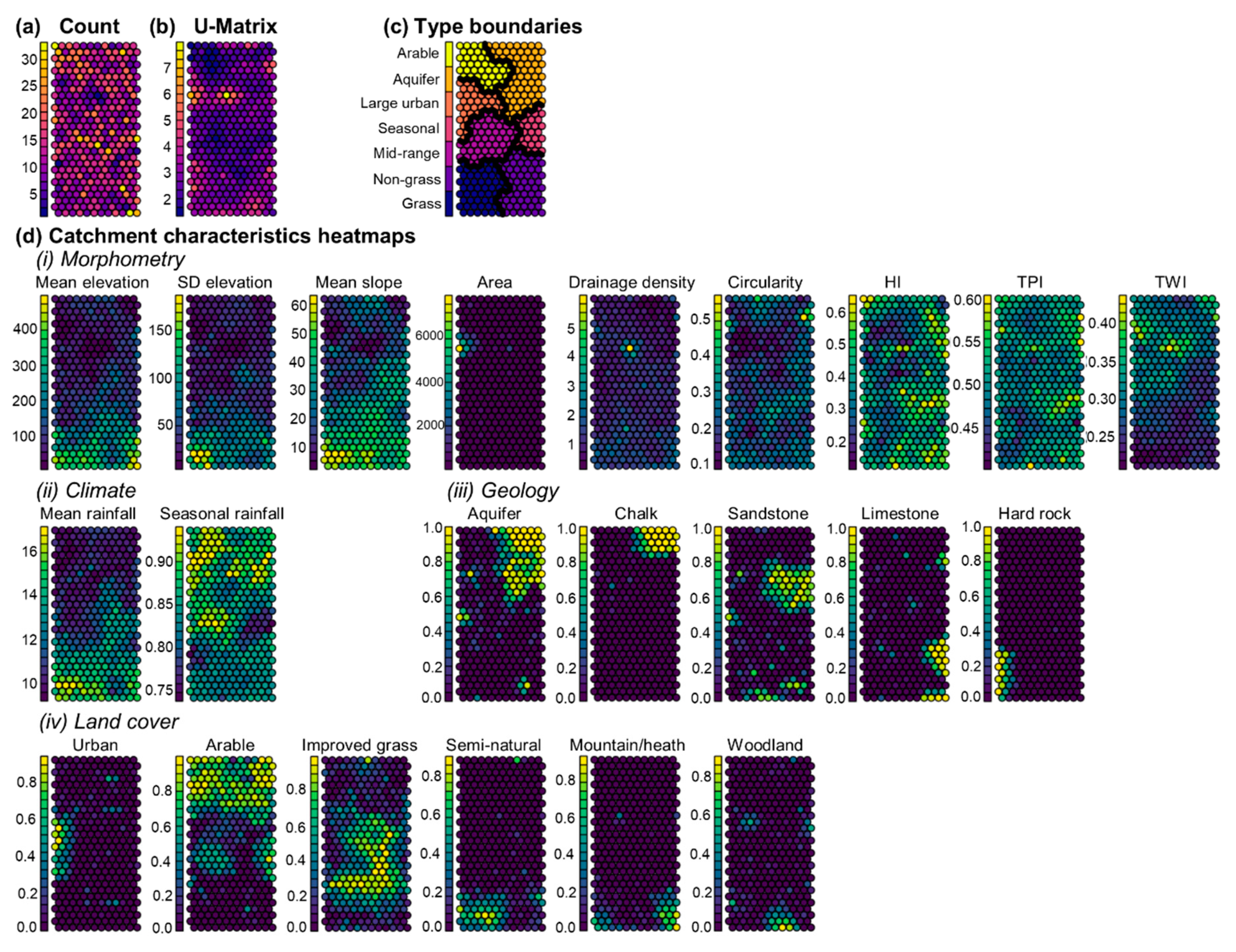
The SOM output was assessed using several measures (Figure 1) overlain on the same grid. The grid represents the topological configuration of the waterbodies based on their catchment characteristics, where each grid cell contains several waterbodies (between 1 and 34 waterbodies) with similar characteristics (Figure 1a). The topological configuration of the map means that waterbodies in each grid cell are most similar to those in neighbouring grid cells, depicted by the U-matrix in Figure 1b, where low values indicate that the grid cell is similar to neighbouring grid cells.
Hierarchical clustering was applied to the SOM output to identify typology classes. The decision of which number of classes to use depended on the intended purpose, as successful typologies must be interpretable to be fit for purpose [3]. Here, seven clusters were selected based on the Davies–Bouldin index, a statistical measure of clustering quality, and because seven clusters sufficiently captured the complexity of catchment characteristics that influenced river functioning whilst remaining interpretable (see Appendix A for further discussion relating to the number of clusters chosen).
The final waterbody type boundaries are presented in Figure 1c for comparison with the SOM heatmaps (Figure 1d). The heatmaps show the distribution of values for each morphometric, climatic, geological and land cover characteristic across the SOM grid (Figure 1d). They indicated a gradient from upland to lowland waterbodies, from the bottom to the top of the heatmaps. At the upland end of the gradients there was higher elevation, slope and rainfall, greater run-off (indicated by the topographic wetness index, TWI), drainage density, seasonal rainfall, harder geologies and more natural land covers, and vice versa for the lowland end of the gradient.
Further inspection of the heatmaps indicated additional patterns and anomalies. The morphometric characteristics hypsometric index (HI), topographic position index (TPI) and circularity showed high levels of variation indicating differing degrees of roughness and catchment development [46] across the upland-to-lowland gradient. There was also a secondary gradient from waterbodies with homogenous to heterogenous landscapes running from the left to right-hand side of the heatmaps with higher HI, TPI, circularity, slope and rainfall values on the right. Other anomalies such as extreme high drainage density values that did not sit in the gradient were apparent, along with a group of waterbodies with high percentage urban land cover and high cumulative catchment area on the left-hand side. Differences in the middle of the upland-lowland gradient were also shown in improved grassland land cover and highly seasonal rainfall.
3.2. The Waterbody Typology
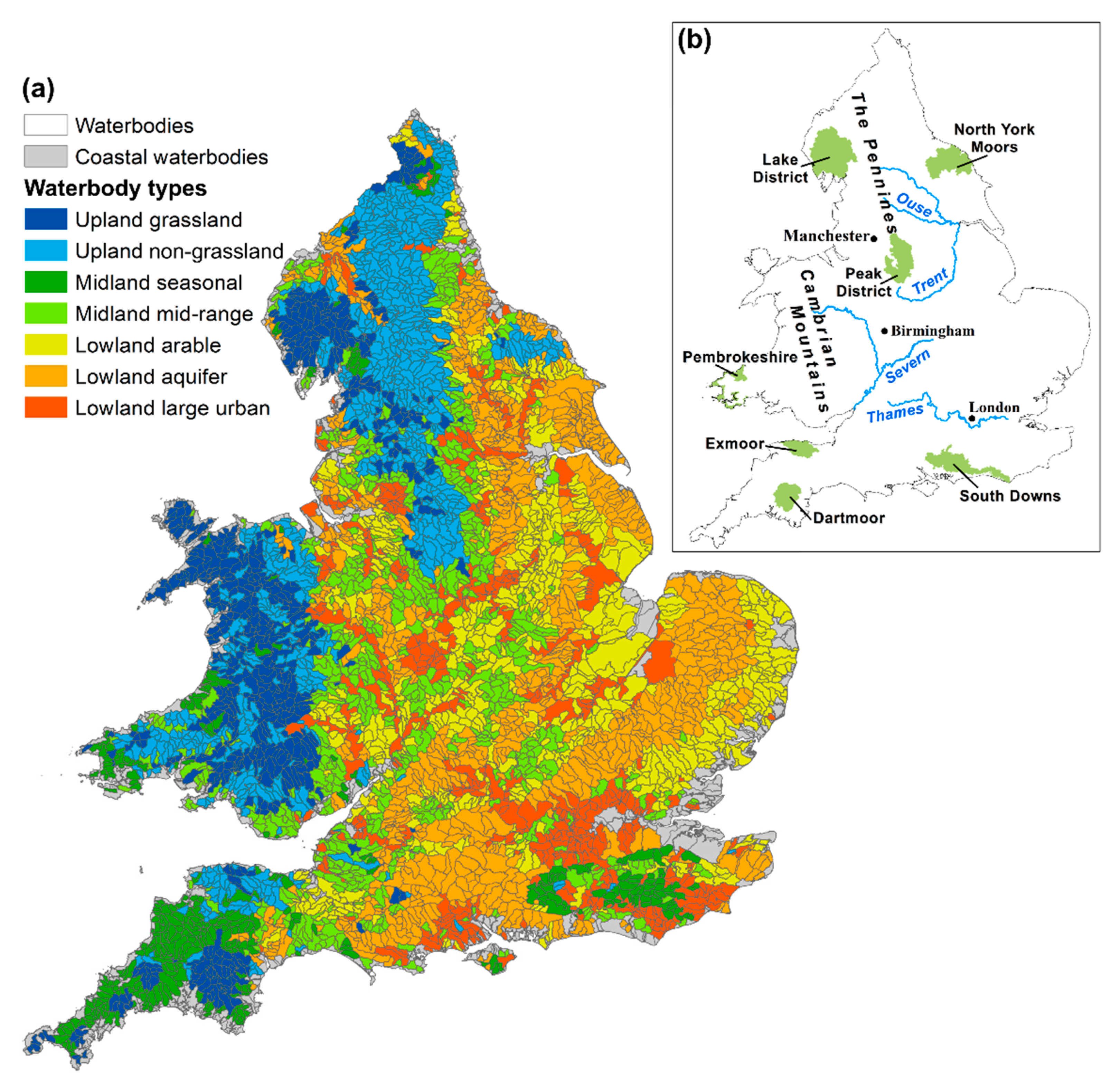
The boundaries of the seven selected waterbody types are displayed in Figure 1c in relation to their catchment characteristics and are named based on the interpretation of the authors. The typology was mapped across England and Wales in Figure 2a. The seven types fit into three broader categories—upland, midland and lowland—based on the dominant upland-lowland gradient displayed in the heatmaps in Figure 1d.
3.2.1. Upland Waterbody Types
Upland waterbody types were defined by high elevation (over 350 m), slope (over 50°) and rainfall (over 14 days with > 1 mm rainfall a year) (Figure 1d). Both upland types exhibited high U-Matrix values (Figure 1b) indicating that waterbodies within upland waterbodies were diverse within this overall gradient.
Upland grassland types (n = 608) were distinguished as having the highest slope and standard deviation of elevation values, lowest TWI and are dominated by natural grassland and hard rock geology (Figure 1d). This suggests deep valleys in a steep impermeable landscape with high levels of runoff. This type is predominantly located in the Lake District, Cambrian Mountains and Dartmoor (Figure 2).
Upland nongrassland types (n = 824) had higher circularity, HI and TPI values (Figure 1d) indicating a more rugged, heterogenous landscape dominated by hillslope processes [46]. This type had limestone geology and mountainous, heath, bog and woodland land covers and was located in the Pennines, North York moors and Exmoor (Figure 2).
3.2.2. Midland Waterbody Types
Midland types were more internally homogenous than upland or lowland types (Figure 1b). Both midland types had similar mean elevations (about 150–250 m) and were dominated by similar geologies, improved grassland and arable landcovers. Differences were primarily in the morphometric and climatic characteristics (Figure 1d).
Midland seasonal types (n = 351) had highly seasonal rainfall with higher slopes, rainfall, circularity, HI and TPI compared to midrange types (Figure 1d). Seasonal waterbodies were the least numerous, limited to the South Downs, the South West and Pembrokeshire (Figure 2).
Midland midrange types (n = 732) had lower slopes and were less rugged landscapes. They had less rainfall that was less seasonal. This type had a wide spatial distribution often adjacent to upland types or representing comparatively upland areas in central England (Figure 2).
3.2.3. Lowland Waterbody Types
Lowland types had lower elevation, slope and rainfall than other types. Lowland arable types (n = 681) had the lowest elevation and rainfall. They were dominated by arable land covers (~80% cover) and high TWI indicating low floodplain locations. There was little variation in catchment characteristics within this type (Figure 1b). Arable types were evenly distributed across the country in the floodplain areas of major rivers and dry, low-lying areas on the east coast (Figure 2).
Aquifer types (n = 892) had more diversity within the class than arable waterbodies (Figure 1b), despite also being dominated by arable land. This is likely because the class boundary reflected the aquifer boundary that contained both chalk and sandstone permeable geologies. Aquifer types had low drainage density with a slightly rougher terrain than other lowland classes, indicated by higher slopes, HI, TPI and circularity (Figure 1d). The distribution of aquifer waterbodies followed bands of permeable geology across England (Figure 2).
Large urban types (n = 397) were distinguished by their high percentage of urban land cover (>50%) and large cumulative catchment area, indicating that they are downstream waterbodies. The boundary of this type extended towards the upland end of the heatmap, indicating that large urban conditions occur over a range of mid-to-low elevations and conditions. This is likely why there was higher heterogeneity of characteristics within this category than others (Figure 1b). Large urban waterbodies were centred around large urban settlements such as London, Birmingham and Manchester or large main rivers such as the Ouse, Trent, Severn and Thames and so on (Figure 2).
3.3. River Habitat Differentiation between Types
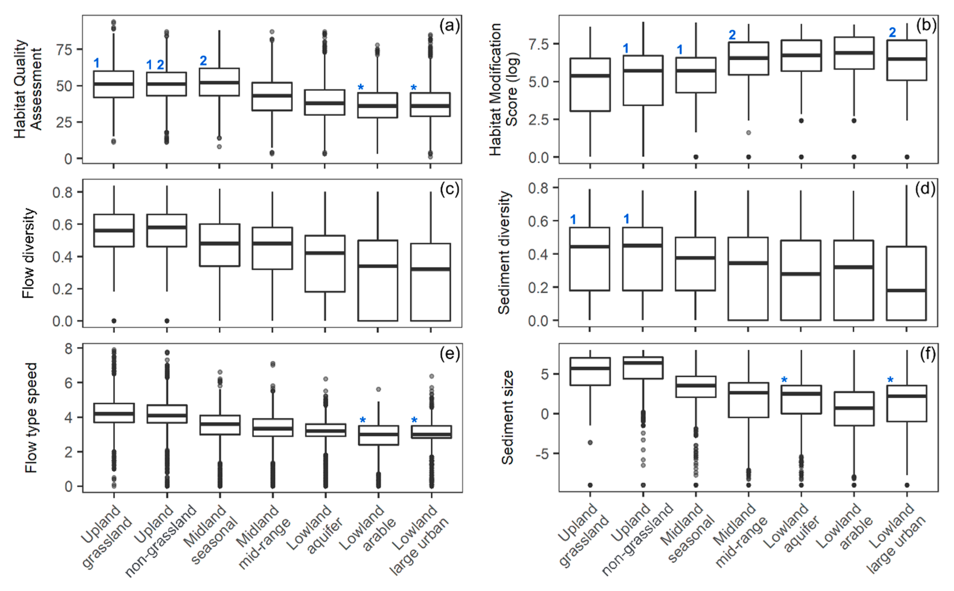
Reach-level characteristics were compared between the seven waterbody types to evaluate whether the summary indices of reach quality and individual physical habitat indices (Table 3) varied between types. All six river habitat indices showed a range of significant differences among waterbody types using the Kruskal–Wallis test (p < 0.01). The Dunn post hoc test indicated that most waterbody types had significantly different indices from one another (p < 0.05; Figure 3).
Flow type speed, sediment size and flow type diversity differed significantly between all types (Figure 3c,e,f). Their distributions predominantly reflected the upland-lowland gradient in waterbody types, with coarser sediments and faster and more diverse flow types in upland waterbody types. Lowland arable waterbodies tended to have the lowest index values of the three lowland types for these indices.
Sediment diversity also exhibited an upland-lowland trend, although there were no significant differences in diversity between the two upland classes (Figure 3d). Sediment diversity values were lowest in large urban waterbodies despite lowland arable types exhibiting lower sediment sizes (Figure 3f).
For both flow indices (Figure 3c,e), there was a steady decline in index value through the waterbody types. For sediment indices, there was a larger difference between seasonal and midrange types that was less evident in the flow indices (Figure 3d,f). Sediment size was also greater in upland nongrassland than upland grassland waterbodies (Figure 3f).
The summary indices, HQA and HMS (Figure 3a,b), also reflected the upland-to-lowland gradient with high habitat quality and low modification scores in upland sites compared to lowland sites. There were more similarities in summary indices between waterbody types than for the individual habitat indices. HQA was not significantly different between the upland grassland, upland nongrassland or midland seasonal types, and HMS was not significantly different between midland midrange and lowland large urban waterbodies, with lowland arable waterbodies exhibiting the greatest modification scores (Figure 3b).
While there were many statistically significant differences between waterbody types, Figure 3 also highlights the broad range of river habitat indices within each type.
4. Discussion
4.1. A Practical and Applicable Typology of Catchment Controls for Waterbodies in England and Wales
Selected catchment controls have been used in previous applied typologies to delineate homogenous river sections [2,11], but the associations between catchment controls, and the response of river reaches to their combined effects, is often not considered. The typology presented here is less focused on classifying reach processes for local management than previous typologies. Instead, the typology was designed to capture multiple catchment controls and their associations for identifying natural boundaries in catchment functioning for strategic management at the national level.
The typology of catchment controls, developed using the SOM approach for waterbodies in England and Wales, was successful at differentiating between key features of the landscape including national reserves, topographical and geological features, major rivers and urban centres (Figure 2). The approach incorporates multiple catchment characteristics that have a functional control on river reaches (Table 2) rather than being limited to only characteristics that are not correlated with one another. Furthermore, the typology boundaries are based on naturally occurring thresholds in the data identified by the clustering algorithm rather than arbitrary boundaries.
These factors likely explain why this waterbody typology differentiates habitat features between types better than the current WFD System A typology. When evaluated against flow type, substrate size and geomorphic activity indices derived from seminatural RHS sites, 0% of WFD System A types were statistically different to all the other types (at a significance level of p < 0.05, [22]). However, in this typology, using the same level of significance, up to 100% of types produced statistical differences in habitat indices between all other types (Figure 3), including 42–57% for the summary indices used to assess the quality of reaches. This indicates that this typology has relevance for river managers and conceptually improves upon the current WFD System A typology, which is based solely on elevation, catchment area and geology (Table 1) and has arbitrary boundaries between categories [20].
The strength of this typology is the range of catchment characteristics included that often showed cross-correlations (Figure 1d). Cross-correlation makes it difficult to isolate individual effects from catchment controls as they interact [26]. This is because catchment controls are not independent [21]; therefore, grouping waterbodies with similar controls is beneficial rather than relying on a single control to describe all catchment influences.
The inclusion of multiple characteristics was possible because the SOM method was adopted. This and other machine learning techniques are becoming more prevalent in multivariate analysis as they can deal with natural artefacts of many environmental datasets, which often make multivariate environmental analyses challenging [26]. The heatmap outputs from the SOM (Figure 1d) also allow for easy visualisation of variable distributions, positive and negative correlations between variables such as the upland-lowland gradient, and anomalies such as the higher drainage density anomaly in the large urban type [28,72].
4.2. Critique of the Typology
Whilst the waterbody typology shows promising differentiation between landscape (Figure 2) and reach features (Figure 3), its limitations must be understood to ensure it is not applied for management in ways that are inappropriate given its design. The most obvious example of limitations is the wide ranges of habitat index values within each waterbody type, despite overall significant differences between most types (Figure 3). As the aim of this paper was to create a waterbody typology that can be applied widely, this is expected, but reasons for these variations are discussed below to highlight limitations of the typology.
The variation in characteristics within waterbody types was greatest in aquifer, large urban and both upland types (Figure 1b). Creating more types may capture more variation, and the selection of the number of types in any typology is ultimately subjective [15,24] but is aided by statistical measures and expert opinion (for the methods used here, see Appendix A). An interpretable classification will never capture the whole range of variation of its population, nor is it expected to, but it must capture enough variation to be fit for purpose. As discussed above, we believe that seven types are appropriate to capture the variation in catchment controls at this national level, evidenced by evaluating the types against survey data (Figure 3).
The limitations of the RHS dataset, used here to represent reach features, should also be noted. The RHS was not designed as a geomorphological survey to capture dynamic process [73] but does include the presence/absence of features that are useful to estimate dominant channel habitat conditions over a standardised 500 m reach. The identification of dominant features present at each transect in the survey means that the diverse conditions of the reach may be underestimated, which may mute more extreme differences between waterbody types. However, although the RHS is not detailed, it does provide a wide spatial coverage with a consistent methodology that makes it a valuable tool for use in national typologies [19,23].
The waterbodies used as the unit for the typology developed here are much larger than reach or subreach units employed by bottom-up typologies (e.g., [2,11,18]), which has practical benefits. For example, the resolution of the GIS-derived datasets used to build the typology can be relatively coarse, and there are numerous RHS surveys available within each waterbody type to effectively evaluate the typology. The waterbody unit also reflects policy units that are widely applied in river management in Europe [12] providing a continuous typology across the landscape not possible if relying on survey data alone. However, the use of waterbodies as subunits of the wider catchment means that controls from upstream of the waterbody are not considered. Only the cumulative catchment area characteristic indicates the position of the waterbody within the wider catchment, which contributed to the large urban waterbody type, separating waterbodies at the downstream end of catchments from other waterbody types. The use of a relatively large study unit also means that variation will be present within types because each waterbody contains a range of processes and local pressures, such as sediment mining, dams and channelization, that are not included in the typology, which is a limitation of this methodology. The aim of this typology, however, was to capture the catchment controls that influence the reach, rather than directly classifying reach processes and features such as channel stream power, slope and planform, which have been the focus of previous top-down and bottom-up typologies (e.g., [2,18,24]). For increased utility of this typology for operational river management at a more local level, data on controls and characteristics at the reach-level should be integrated into the waterbody typology.
The typology also is a temporary snapshot of catchment controls, which is often a critique of river typologies [3]. While many catchment characteristics change over long timescales, such as morphometry or geology (~102 to 104 years), some characteristics are more temporally dynamic such as land cover and rainfall patterns (~101 to 102 years [5]). This is addressed to some extent by taking a long-term average of rainfall (from 1961 to 2016) and a land cover map for the time period most relevant to the validation surveys (2007). While this is not ideal, the top-down nature of this approach means the typology can easily be updated at a relatively inexpensive cost to the user as, and when, major landscape alterations are made or when new data become available. The typology is also evaluated with RHS surveys occurring over a long time period (1994 to 2015) each providing a snapshot of river features that change ~10−1 to 101 years rather than the long-term changes of the catchment controls. Although the link between catchment changes and channel features is complex, the fact the typology performs well when evaluated against over twenty years’ worth of surveys suggests that the typology is relevant over long time periods.
Whilst there are limitations, primarily as a result of the selection of the top-down approach, the validation of the waterbody typology with reach-level data not only creates a useful typology tool with distinctive classes but enhances understanding catchment controls on reach habitats. The top-down method means that this approach can be applied to any waterbody with available data, without expensive and systematically biased surveys. However, the broad distribution of habitat features within each type (despite statistically significant differences; Figure 3) emphasises that this typology is not substitute for detailed surveys and monitoring, but a means of assessing the spatial distribution of catchment controls at a national level. Future work should compare different datasets that reflect other aspects of the geomorphology or ecology of the channel to this typology.
4.3. Gradients and Anomalies in Waterbody Types and Reach Responses
The waterbody types show distinctive distributions of catchment controls reflecting dominant upland-lowland and secondary topographic heterogeneity gradients. Anthropogenic controls often follow these gradients but can occur independently. The response of habitat indices to the waterbody types reflects the gradients observed in the catchment controls.
4.3.1. Upland-Lowland Gradient
Many bottom-up typologies derived from RHS data detect a regional upland-lowland gradient using elevation and distance in the network [19]. In addition, others also found factors such as geology, climate and mean catchment slope to be useful descriptors of regional river habitat patterns [14,23,38,39]. Those that considered anthropogenic catchment pressures found them to only have a weak effect on habitat features [14,74]. We also observe an upland-lowland gradient present across morphometric, climatic, geological and anthropogenic catchment characteristics of England and Wales (Figure 1d and Figure 2), which justifies the validity of a multivariate typology.
The upland-lowland gradient across most characteristics is because of dependency between catchment characteristics that dictates the discharge of water and sediment to the channel [21] altering physical habitat features [75]. The results indicate upland to lowland variation in a variety of processes that are strongly related to geology and topography, including reductions in sediment transport capacity, lower magnitude and frequency hydrographs and, perhaps most importantly, increasing anthropogenic pressures from upland to lowland waterbodies [76]. This is reflected in the habitat indices that decrease in habitat condition from upland to lowland (Figure 3). The distinct separation of habitat indices between each waterbody type, including the midland types, highlights the need to consider rivers along a gradient and not just upland or lowland polarisations.
4.3.2. Heterogeneity Gradient
While the upland-lowland gradient is dominant both in explaining patterns of catchment characteristics (Figure 1d) and habitat indices distributions (Figure 3), a secondary gradient is identified in this waterbody typology. It is a gradient of topographic heterogeneity, driven by patterns in HI, TPI, land cover and geology. Previous studies identified an energy gradient within catchments, from upstream to downstream, as a secondary gradient [19,39]. The distribution of energy within catchments is widely considered a key factor in distributions of geomorphological forms and processes [77] and ecological communities [78,79]. However, this typology is at a broader spatial level, so internal waterbody variations are not accounted for. This emphasises the heterogeneity gradient that has not before been identified nationally. It shows that fluvial processes vary at the same point along the upland-lowland gradient as a result of landscape heterogeneity.
The heterogeneity gradient is related to energy, reflecting regional patterns of process. Heterogenous waterbody types are more circular indicating flashier hydrographs [48], have greater local ruggedness indicating greater coupling to hillslopes and flood responses [43,77] and greater hypsometric integrals suggesting greater dominance of hillslope processes [46] than their counterparts at the same point in the upland-lowland gradient (Figure 1d). These morphometric variables are dependent on climate and geology [21], which create deviations from the upland-lowland gradient, such as higher elevation landscapes in lowland waterbody types as a result of the permeable geology, more easily eroded landscapes in upland limestone waterbodies and more seasonal rainfall producing flashier flood hydrographs in some midland waterbodies [50]. The permeable geology and natural, diverse land covers may also stabilise the hydrograph [51], creating a complex range of processes that are less prominent in the homogenous waterbody types that are dominated by fluvial processes and anthropogenic land covers.
Catchments with a more variable topography are predicted to produce reaches with greater geomorphic heterogeneity [44]. We also observe this as heterogeneous waterbody types tend to exhibit better habitat conditions than their counterparts at the same point in the upland-lowland gradient (Figure 3). Others have also observed differences at similar points along the upland-lowland gradient; Holmes et al. [23] found different macrophyte species at similar elevations, which they attributed to geological differences. However, the heterogeneity gradient better explains the processes that influence reaches, which are as a result of driving variables such as geology and climate. This highlights the utility of using multiple catchment characteristics, particularly morphometry, when exploring catchment controls opposed to solely measures of the upland-lowland gradient, which do not capture the range of processes occurring regionally at similar elevations (Figure 1d).
4.3.3. Anthropogenic Consistencies and Anomalies
Integrated catchment management often focusses on anthropogenic controls, particularly pressures from agricultural and urban land [80], but anthropogenic activity may be hard to distinguish from the upland-lowland gradient [10], as arable land dominates in lowland waterbodies (Figure 1d). Urban land cover crosses a range of low-to-mid elevations suggesting partial independence from the upland-lowland gradient, although it is less dominant in upland rural regions [76]. Large urban types are, however, located at the homogeneous end of the heterogeneity gradient, likely because of limited topographic variability and the location of urban centres in large floodplains dominated by fluvial processes (Figure 1d).
While anthropogenic land covers reflect gradients in more natural catchment characteristics, habitat indices vary between waterbody types dominated by these land covers. In some cases, habitat indices reflect this gradient, for example, aquifer waterbodies that are dominated by arable land cover but are heterogenous frequently have higher habitat indices than other lowland waterbodies (Figure 3). This was also reported in Holmes et al.’s [23] macrophyte typology and is expected as groundwater streams are often characterised by their gravel beds, moderate flow and relatively steep gradient [81].
In contrast, lowland arable types frequently have the finest sediments (Figure 3f), expected partly because of sediment fining associated with the upland-lowland gradient [14], but also because of increases in fine sediment from agricultural practices [54] and the widening and deepening of agricultural drainage ditches that create depositional environments [82]. Arable type waterbodies also have the highest modification score, which follows the upland-lowland gradient, but is surprising as large urban waterbodies commonly have modifications for flood and erosion protection [52,83]. Yet, large urban waterbodies have the lowest diversity scores (Figure 3c,d), often with homogenous flow and sediments, because of management practices such as over-widening, straightening and dredging for flood protection in urban centres [52]. It is, therefore, critical to consider anthropogenic catchment controls in the context of wider catchment processes as they may exaggerate or resist underlying natural gradients.
5. Conclusions
The typology developed and presented here is designed to reflect multiple catchment controls on river reaches, a development on previous typologies that classify reach features using survey data and only consider a subset of possible catchment controls. The use of SOMs combined with hierarchical clustering on this wide range of catchment characteristics has produced a national-level waterbody typology map for 4485 waterbodies in England and Wales.
The typology shows clear differentiation of key landscape features—such as urban centres, national parks, geological features and topographic gradients—and river habitat indices extracted from the RHS dataset. The typology was evaluated with survey data and found to have functional significance, making it valuable for understanding catchment controls on reach features that are important to river managers. The top-down approach utilising solely GIS-derived data allows the typology to be continuous and easily revised as datasets are updated. The same methodology can be applied to other countries with available GIS data and monitoring data for validation. It is, therefore, clear that top-down approaches can be useful in river typologies, allowing the controls on rivers to be classified rather than just the responses to provide an additional layer of understanding.
The typology map in Figure 2 may provide a useful tool for useful assessment of catchment controls in waterbodies, including the type of characteristics that may be influencing the river systems and broad habitat conditions. It can be rapidly applied without the need for time-consuming or expensive surveys to assess the spatial distribution of catchment controls at a national level to aid more strategic management. Integration with more local data is also possible and would increase the utility of the typology from an operational perspective to river management. Although it is not a substitute for detailed surveys and monitoring, the use of field surveys in conjunction with this broad representation of functional catchment controls should enable for a holistic assessment of catchment controls on river reaches. This may discourage a “one-size fits all” approach to river management and offers a step towards better integrated catchment management.
Author Contributions
Conceptualization, E.L.H. and N.J.C.; methodology, E.L.H., J.D.A.M. and M.A.C.; formal analysis, E.L.H.; investigation, E.L.H.; writing—original draft preparation, E.L.H.; writing—review and editing, E.L.H., J.D.A.M., N.J.C. and M.A.C.; visualization, E.L.H.; funding acquisition, E.L.H. All authors have read and agreed to the published version of the manuscript.
Funding
This research was funded by Natural Environmental Research Council (NERC), grant number NE/L002485/1. E.L.H. is the recipient of the funding.
Acknowledgments
The authors would like to thank the Environment Agency and the Centre for Ecology and Hydrology for access to the data used in this paper. The River Habitat Survey data and WFD waterbody boundaries can be access through the UK government portal (data.gov.uk). Links to all other datasets used provided in the relevant reference.
Conflicts of Interest
The authors declare no conflicts of interest. The funders had no role in the design of the study; in the collection, analyses, or interpretation of data; in the writing of the manuscript, or in the decision to publish the results.
Appendix A
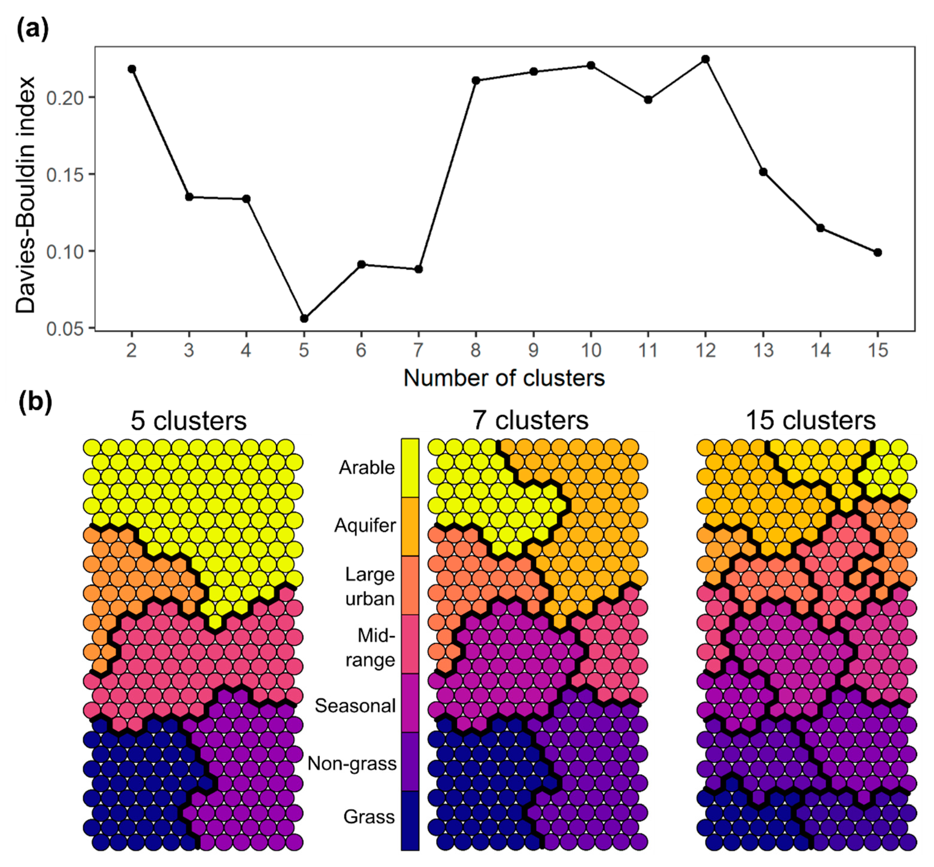
Hierarchical clustering was applied to the SOM output to identify typology classes. The Davies–Bouldin index, a measure of clustering quality, indicates that 5, 7 or 15 clusters are preferable as a result of the low index values (Figure A1a). The index suggests five clusters are statistically optimal, but this number was not selected as the complexity of catchment characteristics that influence river functioning (Table 2) is not sufficiently captured for management purposes. For example, if five clusters are selected, groundwater dominated waterbodies and highly seasonal catchments would not be classified into separate waterbody types (Figure A1b). On the other hand, fifteen clusters reflect subtle variations within types (as indicated by high U-matrix values; Figure 1b) producing a finer classification, primarily along the vertical gradient of the grid (Figure A1b). This additional level of detail does not add much further representation of catchment controls useful for management and so was considered too complicated. Therefore, seven clusters are selected to create seven waterbody types (Figure 1c).
Figure A1.
Identifying the appropriate number of clusters to represent waterbody types. (a) Low Davies-Bouldin Index values indicate the optimum number of clusters. (b) Boundaries of 5, 7 and 15 waterbody types, the numbers of clusters with the lowest Davies-Bouldin index values, plotted on the SOM grid from Figure 1. Seven types were selected based on expert judgement for the intended purpose, described in the text. Names of the selected seven waterbody types reflect the characteristics of the type, see Figure 1.

References
- Frissell, C.A.; Liss, W.J.; Warren, C.E.; Hurley, M.D. A hierarchical framework stream habitat classification. Environ. Manag. 1986, 10, 199–214. [Google Scholar] [CrossRef]
- Brierley, G.; Fryirs, K. River styles, a geomorphic approach to catchment characterization: Implications for river rehabilitation in Bega Catchment, New South Wales, Australia. Environ. Manag. 2000, 25, 661–679. [Google Scholar] [CrossRef]
- Kondolf, G.M.; Montgomery, D.R.; Piégay, H.; Schmitt, L. Geomorphic classification of rivers and streams. In Tools in Fluv. Geomorphol; Kondolf, G.M., Piégay, H., Eds.; Wiley: Chichester, UK, 2003; pp. 171–204. [Google Scholar]
- Hynes, H.B.N. The stream and its valley. Edgardo Baldi Meml. Lect. SIL Proc. 1975, 19, 1–15. [Google Scholar] [CrossRef]
- Gurnell, A.M.; Rinaldi, M.; Belletti, B.; Bizzi, S.; Blamauer, B.; Braca, G.; Buijse, A.D.; Bussettini, M.; Camenen, B.; Comiti, F.; et al. A multi-scale hierarchical framework for developing understanding of river behaviour to support river management. Aquat. Sci. 2016, 78, 1–16. [Google Scholar] [CrossRef] [Green Version]
- Downs, P.W.; Gregory, K.J. River Channel Management: Towards Sustainable Catchment Hydrosystems; Routledge: New York, NY, USA, 2004; ISBN 9780340759691. [Google Scholar]
- Beechie, T.J.; Sear, D.A.; Olden, J.D.; Pess, G.R.; Buffington, J.M.; Moir, H.; Roni, P.; Pollock, M.M. Process-based principles for restoring river ecosystems. BioScience 2010, 60, 209–222. [Google Scholar] [CrossRef] [Green Version]
- Church, M.; Ferguson, R.I. Morphodynamics: Rivers beyond steady state. Water Resour. Res. 2015, 51, 1883–1897. [Google Scholar] [CrossRef]
- England, J.; Gurnell, A.M. Incorporating catchment to reach scale processes into hydromorphological assessment in the UK. Water Environ. J. 2016, 30, 22–30. [Google Scholar] [CrossRef]
- Allan, J.D. Landcapes and Riverscapes: The influence of land use on stream ecosystems. Annu. Rev. Ecol. 2004, 35, 257–284. [Google Scholar] [CrossRef] [Green Version]
- Rinaldi, M.; Gurnell, A.M.; del Tánago, M.G.; Bussettini, M.; Hendriks, D. Classification of river morphology and hydrology to support management and restoration. Aquat. Sci. 2016, 78, 17–33. [Google Scholar] [CrossRef]
- European Commission Directive 2000/60/EC. Off. J. Eur. Communities 2000, L269, 1–15.
- Acreman, M.; Dunbar, M.; Hannaford, J.; Mountford, O.; Wood, P.; Holmes, N.; Cowx, I.; Noble, R.; Extence, C.; Aldrick, J.; et al. Developing environmental standards for abstractions from UK rivers to implement the EU Water Framework Directive. Hydrol. Sci. J. 2008, 53, 1105–1120. [Google Scholar] [CrossRef] [Green Version]
- Naura, M.; Clark, M.J.; Sear, D.A.; Atkinson, P.M.; Hornby, D.D.; Kemp, P.; England, J.; Peirson, G.; Bromley, C.; Carter, M.G. Mapping habitat indices across river networks using spatial statistical modelling of River Habitat Survey data. Ecol. Indic. 2016, 66, 20–29. [Google Scholar] [CrossRef] [Green Version]
- Tadaki, M.; Brierley, G.; Cullum, C. River classification: Theory, practice, politics. Wiley Interdiscip. Rev. Water 2014, 1, 349–367. [Google Scholar] [CrossRef]
- Wright, J.F.; Moss, D.; Armitage, P.D.; Furse, M.T. A preliminary classification of running-water sites in Great Britain based on macro-invertebrate species and the prediction of community type using environmental data. Freshw. Biol. 1984, 14, 221–256. [Google Scholar] [CrossRef]
- Olden, J.D.; Kennard, M.J.; Pusey, B.J. A Framework for hydrologic classification with a review of methodologies and applications in ecohydrology. Ecohydrology 2012, 5, 503–518. [Google Scholar] [CrossRef] [Green Version]
- Rosgen, D.L. A Stream Classification System; Technical Report for Riparian Ecosystem and Their Management: Reconciling Conflicting Uses; First North American Riparian Conference; USDA Forest Service: Washington, DC, USA, 1985.
- Jeffers, J.N.R. Characterization of river habitats and prediction of habitat features using ordination techniques. Aquat. Conserv. Mar. Freshw. Ecosyst. 1998, 8, 529–540. [Google Scholar] [CrossRef]
- UKTAG. Guidance on Typology for Rivers for Scotland, England and Wales; UK Technical Advisory Group Water Framework Directive Work Progress Task 2a; Typology Rivers 2003; pp. 1–4. Available online: http://www.wfduk.org › files › Media › Rivers typology_Final_050603 (accessed on 11 May 2016).
- Schumm, S.A.; Lichty, R.W. Time, space, and causality in geomorphology. Am. J. Sci. 1965, 263, 110–119. [Google Scholar] [CrossRef]
- Naura, M.; The River Restoration Centre, Cranfield, UK; Walker, J.; Environment Agency, Lancashire, UK; Maas, G.; Environment Agency, Cheshire, UK. Derivation and Comparison of Various Typologies for the WFD; UK Technical. Advisory Group Paper Number: RTT. 2003. Personal communication, 1 October 2018. [Google Scholar]
- Holmes, N.T.H.; Boon, P.J.; Rowell, T.A. A revised classification system for British rivers based on their aquatic plant communities. Aquat. Conserv. Mar. Freshw. Ecosyst. 1998, 8, 555–578. [Google Scholar] [CrossRef]
- Bizzi, S.; Lerner, D.N. Characterizing physical habitats in rivers using map-derived drivers of fluvial geomorphic processes. Geomorphology 2012, 169, 64–73. [Google Scholar] [CrossRef]
- Liakos, K.G.; Busato, P.; Moshou, D.; Pearson, S.; Bochtis, D. Machine learning in agriculture: A review. Sensors 2018, 18, 2674. [Google Scholar] [CrossRef] [Green Version]
- Feld, C.K.; Segurado, P.; Gutiérrez-Cánovas, C. Analysing the impact of multiple stressors in aquatic biomonitoring data: A ‘cookbook’ with applications in R. Sci. Total Environ. 2016, 573, 1320–1339. [Google Scholar] [CrossRef] [PubMed]
- Kohonen, T. Self-organized formation of topologically correct feature maps. Biol. Cybern. 1982, 43, 59–69. [Google Scholar] [CrossRef]
- Astel, A.; Tsakovski, S.; Barbieri, P.; Simeonov, V. Comparison of self-organizing maps classification approach with cluster and principal components analysis for large environmental data sets. Water Res. 2007, 41, 4566–4578. [Google Scholar] [CrossRef] [PubMed]
- Walley, W.J.; Martin, R.W.; O’Connor, M.A. Self-Organising Maps for the classification and diagnosis of river quality from biological and environmental data. In IFIP—The International Federation for Information Processing; Springer: Boston, MA, USA, 1999; pp. 27–41. [Google Scholar]
- Morris, D.G.; Flavin, R.W. A digital terrain model for hydrology. In Proceedings of the 4th International Symposium of Spatial Data Handling, Zürich, Switzerland, 23–27 July 1990; pp. 250–262. [Google Scholar]
- Morris, D.G.; Flavin, R.W. Sub-Set of UK 50 m by 50 m Hydrological Digital Terrain Model Grids; NERC, Institute of Hydrology: Wallingford, CT, USA, 1994. [Google Scholar]
- CEH Integrated Hydrological Digital Terrain Model. Available online: https://www.ceh.ac.uk/services/integrated-hydrological-digital-terrain-model (accessed on 2 February 2016).
- Moore, R.V.; Morris, D.G.; Flavin, R.W. Sub-Set of UK Digital 1:50,000 Scale River Centreline Network; NERC, Institute of Hydrology: Wallingford, CT, USA, 1994. [Google Scholar]
- CEH 1:50,000 Digital River Network. Available online: https://www.ceh.ac.uk/services/150000-watercourse-network (accessed on 2 February 2016).
- Perry, M.; Hollis, D. The generation of monthly gridded datasets for a range of climatic variables over the UK. Int. J. Climatol. 2005, 25, 1041–1054. [Google Scholar] [CrossRef]
- Met Office; Hollis, D.; McCarthy, M. UKCP09: Met Office Gridded and Regional Land Surface Climate Observation Datasets; Centre for Environmental Data Analysis. 2017. Available online: https://catalogue.ceda.ac.uk/uuid/319b3f878c7d4cbfbdb356e19d8061d6 (accessed on 10 April 2018).
- BGS Bedrock Geology 1:625,000. Available online: http://www.bgs.ac.uk/products/digitalmaps/DiGMapGB_50.html (accessed on 2 March 2016).
- Harvey, G.L.; Gurnell, A.M.; Clifford, N.J. Characterisation of river reaches: The influence of rock type. Catena 2008, 76, 78–88. [Google Scholar] [CrossRef]
- Vaughan, I.P.; Merrix-Jones, F.L.; Constantine, J.A. Successful predictions of river characteristics across England and Wales based on ordination. Geomorphology 2013, 194, 121–131. [Google Scholar] [CrossRef]
- CEH Morton, R.D.; Rowland, C.S.; Wood, C.M.; Meek, L.; Marston, C.G.; Smith, G.M. Land Cover Map 2007 (25m raster, GB) v1.2. Available online: https://www.ceh.ac.uk/services/land-cover-map-2007 (accessed on 29 February 2016).
- Knighton, D. Fluvial Forms and Processes: A New Perspective, 3rd ed.; Routledge: London, UK, 1998. [Google Scholar]
- Rice, S.P.; Church, M. Grain size along two gravel-bed rivers: Statistical variation, spatial pattern and sedimentary links. Earth Surf. Process. Landf. 1998, 23, 345–363. [Google Scholar] [CrossRef]
- Weiss, A.D. Topographic position and landforms analysis. In Proceedings of the ESRI User Conference, San Diego, CA, USA, 9–13 July 2001. [Google Scholar]
- Benda, L.; Poff, N.L.; Miller, D.; Dunne, T.; Reeves, G.; Pess, G.; Pollock, M. The network dynamics hypothesis: How channel networks structure riverine habitats. BioScience 2004, 54, 413–427. [Google Scholar] [CrossRef] [Green Version]
- Beven, K.J.; Kirkby, M.J. A physically based, variable contributing area model of basin hydrology. Hydrol. Sci. Bull. 1979, 24, 43–69. [Google Scholar] [CrossRef] [Green Version]
- Willgoose, C.; Hancock, G. Revisiting the hypsometric curve as an indicator of form and process in transport-limited catchment. Earth Surf. Process. Landf. 1998, 23, 611–623. [Google Scholar] [CrossRef]
- Miller, V.C. A Quantitative Geomorphic Study of Drainage Basin Characteristics in the Clinch Mountain Area, Virginia and Tennessee 2; Columbia University: New York, NY, USA, 1953. [Google Scholar]
- Gregory, K.J.; Walling, D.E. Drainage Basin Form and Process; Wiley: Chichester, UK, 1973. [Google Scholar]
- Singh, V.P. Effect of spatial and temporal variability in rainfall and watershed characteristics on stream flow hydrograph. Hydrol. Process. 1997, 11, 1649–1669. [Google Scholar] [CrossRef]
- Flores, A.N.; Bledsoe, B.P.; Cuhaciyan, C.O.; Wohl, E.E. Channel-reach morphology dependence on energy, scale, and hydroclimatic processes with implications for prediction using geospatial data. Water Resour. Res. 2006, 42, 1–15. [Google Scholar] [CrossRef]
- Holmes, M.G.R.; Young, A.R.; Gustard, A.; Grew, R. A region of influence approach to predicting flow duration curves within unguaged catchments. Hydrol. Earth Syst. Sci. 2002, 6, 721–731. [Google Scholar] [CrossRef] [Green Version]
- Sear, D.A.; Newson, M.D.; Thorne, C.R. Guidebook of Applied Fluvial Geomorphology; Environment Agency R&D Dissemination Centre: Swindon, UK, 2003. [Google Scholar]
- Dadson, S.J.; Hall, J.W.; Murgatroyd, A.; Acreman, M.; Bates, P.; Beven, K.; Holden, J.; Holman, I.P.; Lane, S.N.; Connell, E.O.; et al. A restatement of the natural science evidence concerning flood management in the UK. Proc. R. Soc. A 2017, 473. [Google Scholar] [CrossRef] [PubMed] [Green Version]
- Wharton, G.; Mohajeri, S.H.; Righetti, M. The pernicious problem of streambed colmation: A multi-disciplinary reflection on the mechanisms, causes, impacts, and management challenges. Wiley Interdiscip. Rev. Water 2017, 4, e1231. [Google Scholar] [CrossRef]
- Kohonen, T. Self-Organizing Maps, 3rd ed.; Springer: Berlin, Germany, 2001; ISBN 9783642569272. [Google Scholar]
- Park, Y.S.; Tison, J.; Lek, S.; Giraudel, J.L.; Coste, M.; Delmas, F. Application of a self-organizing map to select representative species in multivariate analysis: A case study determining diatom distribution patterns across France. Ecol. Inform. 2006, 1, 247–257. [Google Scholar] [CrossRef]
- Vesanto, J. Neural network tool for data mining: SOM toolbox. In Proceedings of the Symposium on Tool Environments and Development Methods for Intelligent Systems, Helsinki, Finland, 18 April 2000; pp. 184–196. [Google Scholar]
- Wehrens, R.; Kruisselbrink, J. Supervised and unsupervised Self-Organising Maps. In Packag. “Kohonen” Version 3.0.7. 2018. Available online: https://cran.r-project.org/web/packages/kohonen/kohonen.pdf (accessed on 4 September 2018).
- R Core Team. A Language and Environment for Statistical Computing; R Core Team: Vienna, Austria, 2018. [Google Scholar]
- Heasley, E.L. Waterbody_Typology Version v1.0.0, Zenodo. 2019. Available online: http://doi.org/10.5281/zenodo.3558120.
- Davies, D.L.; Bouldin, D.W. A cluster separation measure. IEEE Trans. Pattern Anal. Mach. Learn. Intell. 1979, 1, 224–227. [Google Scholar] [CrossRef]
- Raven, P.J.; Fox, P.; Everard, M.; Holmes, N.T.H.; Dawson, F.H. River Habitat Survey: A new system for classifying rivers according to their habitat quality. In Freshwater Quality: Defining the Indefinable? Boon, P.J., Howell, D.L., Eds.; The Stationery Office: Edinburgh, Scotland, UK, 1996; pp. 215–234. [Google Scholar]
- CEN. Water Quality—Guidance Standard for Assessing the Hydromorphological Features of Rivers; European Commission for Standardization: Brussels, Belgium, 2004. [Google Scholar]
- Belletti, B.; Rinaldi, M.; Buijse, A.D.; Gurnell, A.M.; Mosselman, E. A review of assessment methods for river hydromorphology. Environ. Earth Sci. 2015, 73, 2079–2100. [Google Scholar] [CrossRef]
- Harvey, G.L.; Clifford, N.J.; Gurnell, A.M. Towards an ecologically meaningful classification of the flow biotope for river inventory, rehabilitation, design and appraisal purposes. J. Environ. Manag. 2008, 88, 638–650. [Google Scholar] [CrossRef]
- Raven, P.J.; Holmes, N.T.H.; Dawson, F.H.; Everard, M. Quality assessment using River Habitat Survey data. Aquat. Conserv. Mar. Freshw. Ecosyst. 1998, 8, 477–499. [Google Scholar] [CrossRef]
- Davenport, A.J.; Gurnell, A.M.; Armitage, P.D. Habitat survey and classification of urban rivers. River Res. Appl. 2004, 20, 687–704. [Google Scholar] [CrossRef]
- Emery, J.C.; Gurnell, A.M.; Clifford, N.J.; Petts, G.E. Characteristics and controls of gravel-bed riffles: An analysis of data from the river-habitat survey. Water Environ. J. 2004, 18, 210–216. [Google Scholar] [CrossRef]
- Simpson, E.H. Measurement of diversity. Nature 1949, 163, 688. [Google Scholar] [CrossRef]
- Benjamini, Y.; Hochberg, Y. Controlling the false discovery rate: A practical and powerful approach to multiple testing. J. R. Stat. Soc. Ser. B (Methodological) 1995, 57, 289–300. [Google Scholar] [CrossRef]
- Office for National Statistics. National Parks—Full Extent Boundaries in Great Britain. Available online: http://geoportal.statistics.gov.uk/datasets/national-parks-august-2016-full-extent-boundaries-in-great-britain (accessed on 20 August 2016).
- ASCE. Artificial Neural Networks in hydrology: Preliminary concepts. J. Hydrol. Eng. 2000, 5, 115–123. [Google Scholar] [CrossRef]
- Newson, M.D.; Clark, M.J.; Sear, D.A.; Brookes, A. The geomorphological basis for classifying rivers. Aquat. Conserv. Mar. Freshw. Ecosyst. 1998, 8, 415–430. [Google Scholar] [CrossRef]
- Jusik, S.; Szoszkiewicz, K.; Kupiec, J.M.; Lewin, I.; Samecka-Cymerman, A. Development of comprehensive river typology based on macrophytes in the mountain-lowland gradient of different Central European ecoregions. Hydrobiologia 2015, 745, 241–262. [Google Scholar] [CrossRef] [Green Version]
- Bunn, S.E.; Arthington, A.H. Basic principles and ecological consequences of altered flow regimes for aquatic biodiversity. Environ. Manag. 2002, 30, 492–507. [Google Scholar] [CrossRef] [Green Version]
- Raven, E.K.; Lane, S.N.; Bracken, L.J. Understanding sediment transfer and morphological change for managing upland gravel-bed rivers. Prog. Phys. Geogr. 2010, 34, 23–45. [Google Scholar] [CrossRef]
- Church, M. Geomorphic thresholds in riverine landscapes. Freshw. Biol. 2002, 47, 541–557. [Google Scholar] [CrossRef] [Green Version]
- Vannote, R.; Minshall, G.; Cummins, K.; Sedell, J.; Cushing, C. The River Continuum Concept. Can. J. Fish. Aquat. Sci. 1980, 37, 130–137. [Google Scholar] [CrossRef]
- Gurnell, A.M.; O’Hare, J.M.; O’Hare, M.T.; Dunbar, M.J.; Scarlett, P.M. An exploration of associations between assemblages of aquatic plant morphotypes and channel geomorphological properties within British rivers. Geomorphology 2010, 116, 135–144. [Google Scholar] [CrossRef]
- Downs, P.W.; Gregory, K.J.; Brookes, A. How integrated is river basin management? Environ. Manag. 1991, 15, 299–309. [Google Scholar] [CrossRef]
- Berrie, A.D. The chalk-stream environment. Hydrobiologia 1992, 248, 3–9. [Google Scholar] [CrossRef]
- Poff, N.L.; Allan, J.D.; Bain, M.B.; Karr, J.R.; Prestegaard, K.L.; Richter, B.D.; Sparks, R.E.; Stromberg, J.C. A paradigm for river conservation and restoration. BioScience 1997, 47, 769–784. [Google Scholar] [CrossRef]
- Walsh, C.J.; Roy, A.H.; Feminella, J.W.; Cottingham, P.D.; Groffman, P.M.; Raymond, P.M. The urban stream syndrome: Current knowledge and the search for a cure. J. N. Am. Benthol. Soc. 2005, 24, 706–723. [Google Scholar] [CrossRef]
Figure 1.
SOM output grids: (a) the number of waterbodies within each grid cell; (b) U-matrix (unified distance matrix) indicating the difference between neighbouring grid cells; (c) waterbody type boundaries identified from the hierarchical clustering analysis. The name attributed to each type is described in the text. (d) Heatmaps of catchment characteristics displayed on the SOM grid (scale bars indicate units of each characteristic shown in Table 2).

Figure 2.
(a) Map of waterbody typology for England and Wales based on the SOM analysis with the names the authors attributed to each type. (b) Location of features in England and Wales that are mentioned in the text (for readers unfamiliar with the geography of England and Wales); green areas indicate national parks [71].

Figure 3.
Distribution of six RHS variables for each waterbody type: (a) HQA; (b) HMS plotted on a log-scale; (c) flow diversity; (d) sediment diversity; (e) flow type speed and; (f) sediment size. Types with no significant difference (p > 0.05) between each other, as a result of the Dunn test, are indicated by numbers. * Indicates distributions with a significant difference of p < 0.05, all other differences p < 0.01.


Table 1.
Comparison of the number of local and catchment controls used to classify reaches and waterbodies (denoted by *) in previous typologies in Great Britain (an X indicates the corresponding control was included in the typology).
Table 1.
Comparison of the number of local and catchment controls used to classify reaches and waterbodies (denoted by *) in previous typologies in Great Britain (an X indicates the corresponding control was included in the typology).
| Local Controls | Catchment Controls | ||||||||||||||
|---|---|---|---|---|---|---|---|---|---|---|---|---|---|---|---|
| Site altitude | Site slope | Distance to source | Height of source | Channel geometry | Stream power | Discharge | Floodplain width | Elevation | Upstream area | Geology | Climate | Baseflow Index | Morphometry | Land cover | |
| Jeffers [19] | X | X | X | X | |||||||||||
| Holmes et al. [23] | X | X | X | X | |||||||||||
| WFD System A [20] * | X | X | X | ||||||||||||
| Acreman et al. [13] * | X | X | X | ||||||||||||
| Bizzi and Lerner [24] | X | X | X | X | |||||||||||
| This typology * | X | X | X | X | X | X | |||||||||
Table 2.
List of GIS-derived catchment characteristics used to create the typology and description of their control on river functioning. Units and source for the method are indicated where appropriate.
Table 2.
List of GIS-derived catchment characteristics used to create the typology and description of their control on river functioning. Units and source for the method are indicated where appropriate.
| Catchment Characteristic | Units | Control on River Functioning |
|---|---|---|
| Morphometry | ||
| Cumulative catchment area | km2 | |
| Mean slope | degrees | |
| Mean elevation | m | |
| Standard deviation elevation | m | |
| Topographic Position Index (TPI) | 0–1 | |
| Topographic Wetness Index (TWI) | 0–1 | |
| Drainage density | km/km2 | |
| Hypsometric Index (HI) | 0–1 | |
| Circularity ratio | 0–1 | |
| Climate | ||
| Mean annual number of days with rain > 1 mm | n | |
| Seasonal rainfall ratio | 0–1 | |
| Geology | ||
| Hard rock | % |
|
| Other limestone | % | |
| Sandstone | % | |
| Chalk | % | |
| Aquifer | % | |
| Land cover | ||
| Woodland | % |
|
| Improved grassland | % | |
| Seminatural grassland | % | |
| Mountain, heath, bog | % | |
| Arable | % | |
| Urban | % |
Table 3.
Habitat indices calculated from the national RHS dataset used to evaluate the typology and the ranges of the indices.
Table 3.
Habitat indices calculated from the national RHS dataset used to evaluate the typology and the ranges of the indices.
| Habitat Index | Mean Scores (Range) |
|---|---|
| Summary indices (Overview of reach condition for river quality assessment) | |
| Habitat Quality Assessment (HQA) | 42 (1–94) |
| Habitat Modification Score (HMS) | 1055 (1–7715) |
| Individual habitat indices (Quantify individual components of reach condition that reflect physical habitat) | |
| Flow type diversity | 0.39 (0–0.84) |
| Sediment diversity | 0.30 (0–0.82) |
| Flow type speed | 3.29 (0–7.9) |
| Sediment size | 2.46 (−9–8) |
© 2019 by the authors. Licensee MDPI, Basel, Switzerland. This article is an open access article distributed under the terms and conditions of the Creative Commons Attribution (CC BY) license (http://creativecommons.org/licenses/by/4.0/).
Share and Cite
MDPI and ACS Style
Heasley, E.L.; Millington, J.D.A.; Clifford, N.J.; Chadwick, M.A. A Waterbody Typology Derived from Catchment Controls Using Self-Organising Maps. Water 2020, 12, 78. https://doi.org/10.3390/w12010078
AMA Style
Heasley EL, Millington JDA, Clifford NJ, Chadwick MA. A Waterbody Typology Derived from Catchment Controls Using Self-Organising Maps. Water. 2020; 12(1):78. https://doi.org/10.3390/w12010078
Chicago/Turabian StyleHeasley, Eleanore L., James D. A. Millington, Nicholas J. Clifford, and Michael A. Chadwick. 2020. "A Waterbody Typology Derived from Catchment Controls Using Self-Organising Maps" Water 12, no. 1: 78. https://doi.org/10.3390/w12010078
Note that from the first issue of 2016, this journal uses article numbers instead of page numbers. See further details here.