Analysis of Peak Flow Distribution for Bridge Collapse Sites

Abstract

Bridge collapse risk can be evaluated more rigorously if the hydrologic characteristics of bridge collapse sites are demystified, particularly for peak flows. In this study, forty-two bridge collapse sites were analyzed to find any trend in the peak flows. Flood frequency and other statistical analyses were used to derive peak flow distribution parameters, identify trends linked to flood magnitude and flood behavior (how extreme), quantify the return periods of peak flows, and compare different approaches of flood frequency in deriving the return periods. The results indicate that most of the bridge collapse sites exhibit heavy tail distribution and flood magnitudes that are well consistent when regressed over the drainage area. A comparison of different flood frequency analyses reveals that there is no single approach that is best generally for the dataset studied. These results indicate a commonality in flood behavior (outliers are expected, not random; heavy-tail property) for the collapse dataset studied and provides some basis for extending the findings obtained for the 42 collapsed bridges to other sites to assess the risk of future collapses.

1. Introduction

The common causes categorized for bridge collapses in the USA, as recorded in New York State Department of Transportation (NYSDOT) database, are hydraulic, collision, overload, deterioration, geotechnical, nature, and other [1], with 62.23% of over-water bridge collapses corresponding to hydraulic events, 6.9% to collision, 11.33% to overload, 9.03% to deterioration, 1.48% to geotechnical, 3.28% to nature (storm/hurricane, Earthquake), and 5.75% to other [1]. Hydraulic events, therefore, are perceived to be the common cause of total and partial bridge collapses in the US [1,2,3]. Whereas scouring is the most common hydraulic event for bridge collapse [2], flood-induced scouring is of particular concern due to the intensity of recent floods in the different states of the USA and the associated high risk of safety.

In response to flood risk, engineering design primarily aims at determining the magnitude of floods for a predefined return period. The methods to determine the flood magnitude of the design flood vary, with recommended methods including TR-55 [4], Bulletin 17C [5], and StreamStats [6], among several others. Regardless of the types of methods chosen, analyzing peak flow distribution parameters is not a common practice in bridge design procedures. Nonetheless, the analysis of peak flow distribution parameters provides some basis to reason formally about the counter-intuitive properties of flood events and to identify trends or commonalities among the critical bridge sites.

Peak flow distribution analysis requires the selection of an applicable extreme value distribution fitting approach. There are two approaches: block-maxima, in which a series of annual peak floods are used to directly define an extreme value distribution; and peaks over-threshold (POT), in which distributions are fit to both the frequency of floods above a threshold and their magnitudes. The U.S. Water Resources Council requires the use of log-Pearson type 3 (LP3) distributions for the annual maxima approach, although the generalized extreme value distribution (GEV) seems to be the most widely used model for extreme events [7]. The major benefit of the GEV model is its ability to fit highly skewed data [7]. Therefore, recent hydrologic research has focused on explaining the parameters of the GEV distribution of streamflow extremes [8,9,10,11,12,13,14].

If annual maximum exceedances are assumed to be GEV-distributed, the POT exceedances are assumed to be generalized Pareto (GP)-distributed [15], following recommendations in the field of statistics [16,17]. Fitting the GP distribution to exceedances over a high threshold and also estimating the frequency of exceeding the threshold by fitting a Poisson distribution allows for the simultaneous fitting of parameters concerning both the frequency and intensity of extreme events. Compared to the annual maxima approach, therefore, the main advantage of POT modeling is that it allows for a more rational selection of events to be considered as “floods” and is not confined to only one event per year. The POT approach considers a wide range of events and provides the possibility of controlling the number of flood occurrences to be included in the analysis by appropriate selection of the threshold. However, the POT approach remains under-employed mainly because of the complexities associated with the choice of threshold and the selection of criteria for retaining flood peaks (Lang et al. (1999)). Nonetheless, threshold selection is tightly linked to the choice of the process distribution, to the over-threshold distribution, and to the hypothesis of independence [18].

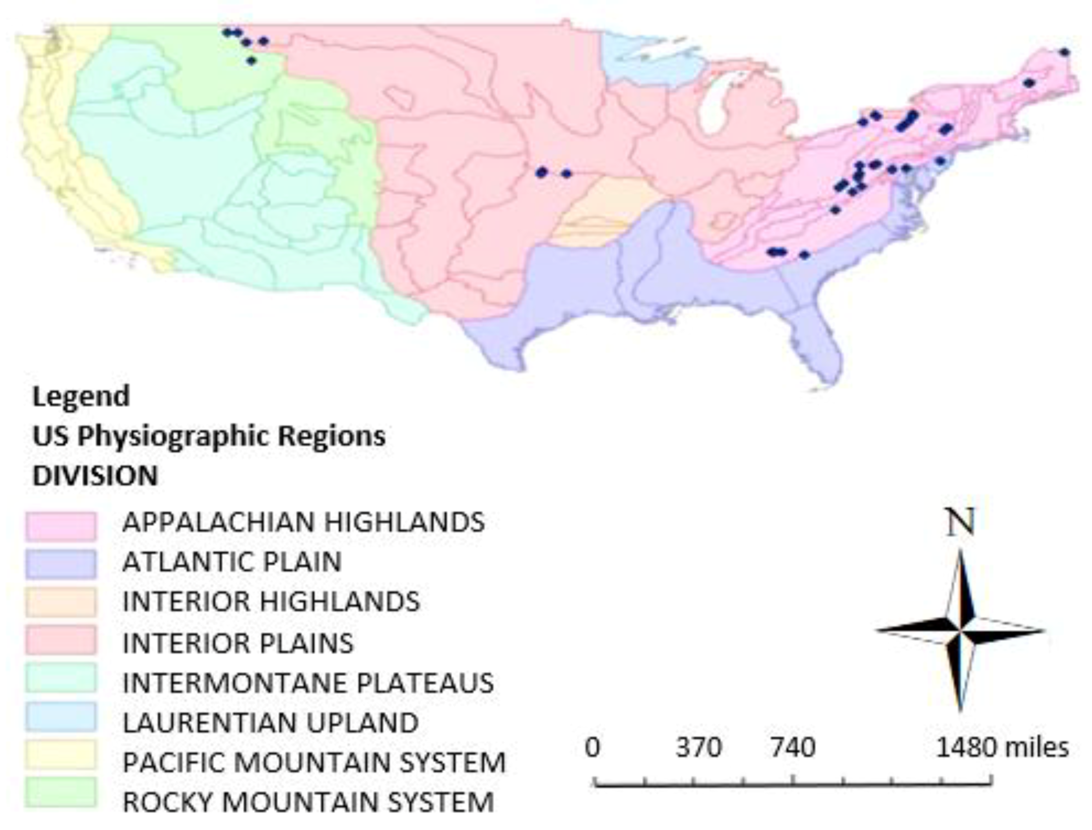
The objectives of this study are: (1) To derive peak flow distribution parameters, (2) to identify trends linked to flood magnitude and flood behavior, and (3) to compare different approaches in deriving return periods for bridge collapse sites. To attain the objectives, this paper presents an analysis of the derived GEV distribution parameters for 42 bridge collapse sites (Figure 1) and also present a comparison of GEV and POT (GP and Poisson) approaches, with a focus on the associated capabilities and uncertainties. Obtained results can reveal any existing trends in the statistical behavior of peak floods in bridge collapse sites, and can support the understanding of the mechanism behind the probabilistic generation of floods. Such analysis provides preliminary data to assess future collapse risk as it can be highlighted that the flood event emergence should be expected in a specific manner (not as a surprising outlier).

2. Methods

2.1. Identification of Bridge Collapse Sites

The New York State Department of Transportation (NYSDOT) bridge failure database (NYSDOT 2014a) is used here to identify 42 bridge collapse sites. NYSDOT is the only US-wide database of bridge collapses. Totally or partially collapsed bridges are added to the database based on journalism databases and surveys of other state DOTs. The recorded information includes identifiers in the National Bridge Inventory, the location of the collapsed bridge, the feature under the bridge, the year of construction, the date or year of collapse, the bridge material and structure type, the type of collapse (total or partial), the number of casualties related to the collapse, and other comments. For this work, the bridges were sought according to the following criteria:

• Existence of a stream gauge listed in the US Geological Survey (USGS) National Water Information System Database.
• The gage station being at the bridge location, near the bridge location (on the same tributary of the river), or at a further distance (not the same tributary, but on the same river).
• Bridges were apparently collapsed (complete or partial collapse) due to floods.

2.2. Flood Frequency Analysis

When conducting a flood frequency analysis, an initial step is to undertake basic analysis of the peak flow and daily flow time series to check for obvious errors that the data conforms to the assumptions used in the frequency analysis.

For peak flows, an autocorrelation test [19] is used to check the validity of the assumption of independence and identical distribution of annual peak flows. This test checks the correlation between values in a one-time step and the value in a previous (and future) time step. Trends in a time series are identified using the Mann–Kendall test [20], which is nonparametric and does not require that the data conform to any specific statistical distribution. This test uses Kendall’s τ as the test statistic (

Table 1. Generalized extreme value distribution (GEV) distribution parameters derived using annual peak flow data from the US Geological Survey (USGS).

Site#	NYSDOT Database Bridge ID/State	USGS Station ID (Sample Size in Superscript)	Basin Area (km2)	GEV Shape Parameter	GEV Location Parameter	GEV Scale Parameter	AIC/BIC	Co-Efficient of Variation of Location Parameter	Kendall’s $\mathit{\tau }$/p Value
1	50/WV 1	0161150095	1,749,990.2	3.1 × 10−1	1.0 × 104	6.8 × 103	2013/2021.3	7.6 × 10−1	−0.05/0.45
2	57/WV 1	0318250088	1398.59	1.4 × 10-1	1.6 × 104	5.9 × 103	1835.1/1842.5	4.1 × 10−1	0.14/0.06
3	118/NJ 1	0146585051	167.05	1.6 × 10−1	630.8	341.1	771.2/777	6.0 × 10−1	0.079/0.42
4	195 */VA 1	0162480030	189.069	1.4 × 10−1	2163.8	1151.2	530.8/535	6.0 × 10−1	0.02/0.89
5	246 */NY 1	0421350077	1129.23	1.7 × 10−1	1.2 × 104	4.6 × 103	1555.1/1562.1	4.3 × 10−1	−0.14/0.09
6	283/GA 1	0221830051	2434.59	2.1 × 10−1	9470.4	5295.9	1054.1/1059.9	6.3 × 10−1	−0.35/0.00027
7	285/GA 1	0221830051	2434.59	2.1 × 10−1	9470.4	5295.9	1054.1/1059.9	6.3 × 10−1	−0.35/0.00027
8	287 */GA 1	0220845045	468.788	0.19	1986.9	1175.1	790.5/795.9	6.8 × 10−1	−0.12/0.27
9	288 */GA 1	0221900045	455.838	2.8 × 10−2	2.9 × 103	1.8 × 103	822.3/827.7	7.1 × 10−1	−0.26/0.01
10	456/MD 1	0164350068	162.65	6.2 × 10−1	2044.7	1077.8	1211.8/1218.5	6.1 × 10−1	0.18/0.03
11	462 */ME 1	0101000067	3473.17	−2.4 × 10−1	23,121.7	7393.6	1389/1395.6	3.5 × 10−1	0.16/0.06
12	503/MT 2	0609170041	229.21	3.6 × 10−1	2249.7	1119.8	727.8/733	0.6	0.03/0.76
13	506/MT 2	0610800063	284.90	1.0	517	587.03	1061/1067.4	1.3	−0.27/0.002
14	512/MT 2	0609320044	229.21	0.48	1005.9	555.45	728.4/733.8	0.6	−0.15/0.16
15	513/MT 2	0609320044	91.17	0.48	1005.9	555.45	728.4/733.78	0.6	−0.15/0.16
16	515/MT 2	0610800063	5599.55	1.0	517	587.03	1061/1067.5	1.3	−0.27/0.002
17	524/MT 3	0606150077	5599.55	0.3	209.4	113.2461	1003.4/1010.4	0.6	−0.04/0.6
18	811 */NY 1	0423900066	326.34	5.3 × 10−2	1.1 × 103	4.2 × 102	1015.6/1022.2	4.4 × 10−1	−0.12/0.17
19	812 */NY 1	0424001066	1411.54	5.3 × 10−2	1.1 × 103	4.2 × 102	1015.6/1022.2	4.4 × 10−1	−0.12/0.17
20	825 */NY 1	0423900066	127.17	5.3 × 10−2	1.1 × 103	4.2 × 102	1015.6/1022.2	4.4 × 10−1	−0.12/0.17
21	826/NY 1	0423300077	499.87	0.34	1022.7	641.11	1270.6/1277.6	7.4 × 10−1	−0.05/0.53
22	829/NY 1	0153033232	233.10	4.3 × 10−1	2.7 × 104	8.4 × 103	712.7/717.1	3.7 × 10−1	−0.17/0.17
23	830/NY 1	0153033232	233.10	4.3 × 10−1	2.7 × 104	8.4 × 103	712.7/717.1	3.7 × 10−1	−0.17/0.17
24	864/NY 1	0423400092	497.28	2.1 × 10−1	2600.3	1010.8	1594.2/1601.7	4.4 × 10−1	−0.09/0.21
25	901 */NY 2	0421650086	99.20	8.3 × 10−2	833	411.2	1321.1/1328.5	0.57	−0.09/0.23
26	904 */NY 2	0421650086	852.11	8.3 × 10−2	833	411.2	1321.1/1328.5	0.57	−0.1/0.22
27	992 */SC 1	0219600074	1686.08	−3.0 × 10−2	9721.1	5403.8	1504.9/1511.9	6.17 × 10−1	−0.14/0.09
28	1044/VA 1	0202150089	266.77	2.8 × 10−1	8100.5	4257.2	1806/1813.5	6.01 × 10−1	0.05/0.48
29	1164/WV 1	0160650091	1,749,990.2	5.1 × 10−1	1.1 × 104	6.3 × 103	1924.3/1931.9	6.63 × 10−1	0.04/0.59
30	1168/WV 1	0160750076	1398.59	6.1 × 10−1	2524.9	1630.5	1425/1432	7.19 × 10−1	−0.28/0.0003
31	1177/WV 1	03182500	1398.6	1.4 × 10−1	1.6 × 104	5.9 × 103	1835.1/1842.5	4.12 × 10−1	0.14/0.06
32	1251/VA 1	0206850089	334.11	2.4 × 10−1	3312.4	2017.6	1670/1677.5	6.93 × 10−1	0.03/0.70
33	1262 */MD 4	0158509023	647.50	6.2 × 10−1	952.4	501.8	365.7/369.1	0.59	0.40/0.01
34	1450 */KS 2	0689235044	3206.41	−3.9 × 10−2	4.9 × 104	3.0 × 104	1043.9/1049.3	0.66	−0.06/0.57
35	1455/KS 2	0688800061	396.27	2.2 × 10−1	4778.3	3794.3	1218.2/1224.6	0.91	0.06/0.49
36	1464/KS 2	0688850065	396.27	2.2 × 10−1	4778.3	3794.3	1218.2/1224.6	0.94	0.06/0.49
37	1482/MD 1	0159650069	57.24	2.2 × 10−1	1319.9	569.3	1118.2/1124.9	4.76 × 10−1	0.01/0.91
38	1484 *MD 1	0161352513	57.24	−2.3 × 10−1	4757.7	1594.1	234.1/235.8	3.70 × 10−1	−0.36/0.1
39	1547 */ME 1	0104600047	3206.41	2.6 × 10−1	2097.8	994.1	811/816.6	5.66 × 10−1	0.009/0.93
40	1548 */ME 1	0104600047	154,767.33	2.6 × 10−1	2097.8	994.1	811/816.6	5.66 × 10−1	0.009/0.93
41	1630/NY 1	0136250086	629.37	4.4 × 10−1	1.1 × 104	7.7 × 103	1844.3/1851.6	7.70 × 10−1	0.07/0.32
42	3619 */NY 1	0136500081	629.37	1.8 × 10−1	2181.3	1224.3	1427/1434.1	6.59 × 10−1	0.03/0.68

* Fail to reject Gumbel distribution. ¹ Appalachian Highland (30 sites). ² Interior plains (10 sites). ³ Rocky Mountain (1 site). ⁴ Atlantic plain (1 site).

) to measure the strength of the monotonic relationship between annual peak streamflow and the year in which it occurred. Positive values for τ indicate the occurrences of annual peak stream flows are increasing with time for the period of record, whereas negative values of τ indicate that the annual peak stream flows are decreasing with time for the period of record. A p-value (Table 1) was also calculated for determining the significance of the τ value. To check whether or not there exists temporal dependence in threshold excess data, extremal index values [21] need to be calculated; extremal index values less than unity imply some dependence, with stronger dependence as the value decreases.

After the initial analysis, three approaches (GEV, GP, and PP) were employed to perform the flood frequency analysis. Each fitted model is evaluated with the Akaike information criterion [22] and the Bayesian information criterion [23] (Table 1). When multiple models are fitted to a specific dataset, each one including different predictor variables, then the model with lower values of AIC and BIC is preferable. It is, therefore, possible to draw conclusions about which approach is best in general or, at least, based on some site characteristics.

2.3. Fitting Distributions

2.3.1. Generalized Extreme Value (GEV)

Whereas in practice, it is very difficult to choose which of the three families of extreme value distributions (Gumbel, Frechet, and Weibull) is the most appropriate for real data, GEV offers a better analysis of block maxima data as it combines three distributions into a single family of models. The cumulative distribution function of the GEV distribution is given by the following equation [24,25,26,27,28].

$$F\left(x/\theta \right)=exp\left(-{\left(1+k\left(\left(x-\mu \right)/\sigma \right)\right)}^{\pm 1/k}\right), \theta = \left(\mu ,\sigma ,k\right), \sigma >0$$

(1)

Here $\mu$ is the location parameter, $\sigma$ is the scale parameter, and k is the shape parameter.

Investigation of large discharge datasets from Central Europe, UK, and USA have focused on estimation of scale, location, and shape parameters [29,30,31,32,33,34], and the most frequently identified empirical relationship is with basin area, particularly for location and scale parameters [8]. The theoretical and empirical justification [9,10,29,30,33,35] of location and scale parameterizations is derived from the concept that “location and scale parameters are mostly related to the magnitude of flow and therefore, mostly depend on the area of the basin [29]”.

The shape parameter is of different nature and is related to the behavior of the upper tail of the distribution, and therefore, is of particular interest to reveal “how extreme” the floods are. Recent studies suggest that the shape parameter depends on climate indices, while other attributes of the catchments are less important [8,9,36,37]. One most recent study [8] examines the nature of the shape parameter across 591 basin characteristics with a large diversity of climate types and find that the most important explanatory variables for shape parameters are mean daily precipitation, frequency of high precipitation days, the precipitation GEV location parameter, and the precipitation GEV shape parameter. With such findings, the GEV shape parameter is most preferably modelled by a normal distribution with a common mean across all sites [8,9,10,35,38]. The shape parameter is also of critical significance in that it proscribes the type of distribution: Gumbel (shape parameter = 0), Frechet (shape parameter >0) and Weibull (shape parameter <0) for fitting to block maxima series of data. Therefore, the shape parameter is related to how extreme the floods are.

2.3.2. Generalized Pareto (GP)

The generalized Pareto (GP) distribution has statistical justification for fitting to excesses over a high threshold [21] and was found to provide a good approximation for daily stream flow data in the USA [39,40,41]. Before fitting the GP distribution to the daily data, it is first necessary to choose a threshold. From literature reviews, three types of tests have been identified for proposing threshold selection. Type I identifies the threshold by fixing the average number of peak exceedances per year [42,43,44,45] or using events only over a given return period [46,47,48]. The Type I test was rejected by Rosbjerg and Madsen (1992) [15] because it apparently disregards the physical properties within the region in the threshold determination. Type II identifies the threshold based on the domain where the mean exceedance above threshold is a linear function of the threshold level [18,49,50]. This test is equivalent to choosing the threshold to maximize the stability of the POT distribution parameter estimates [18]. Type III selects a threshold based on the validity of the Poisson distribution of peak counts [18]. The Type III test is done when distributions are fit to both the frequency of floods above a threshold and their magnitudes, assuming a Poisson distribution of peak counts. Type III test checks the assumption of the Poisson process that the random variable should be independent and should be exponentially distributed.

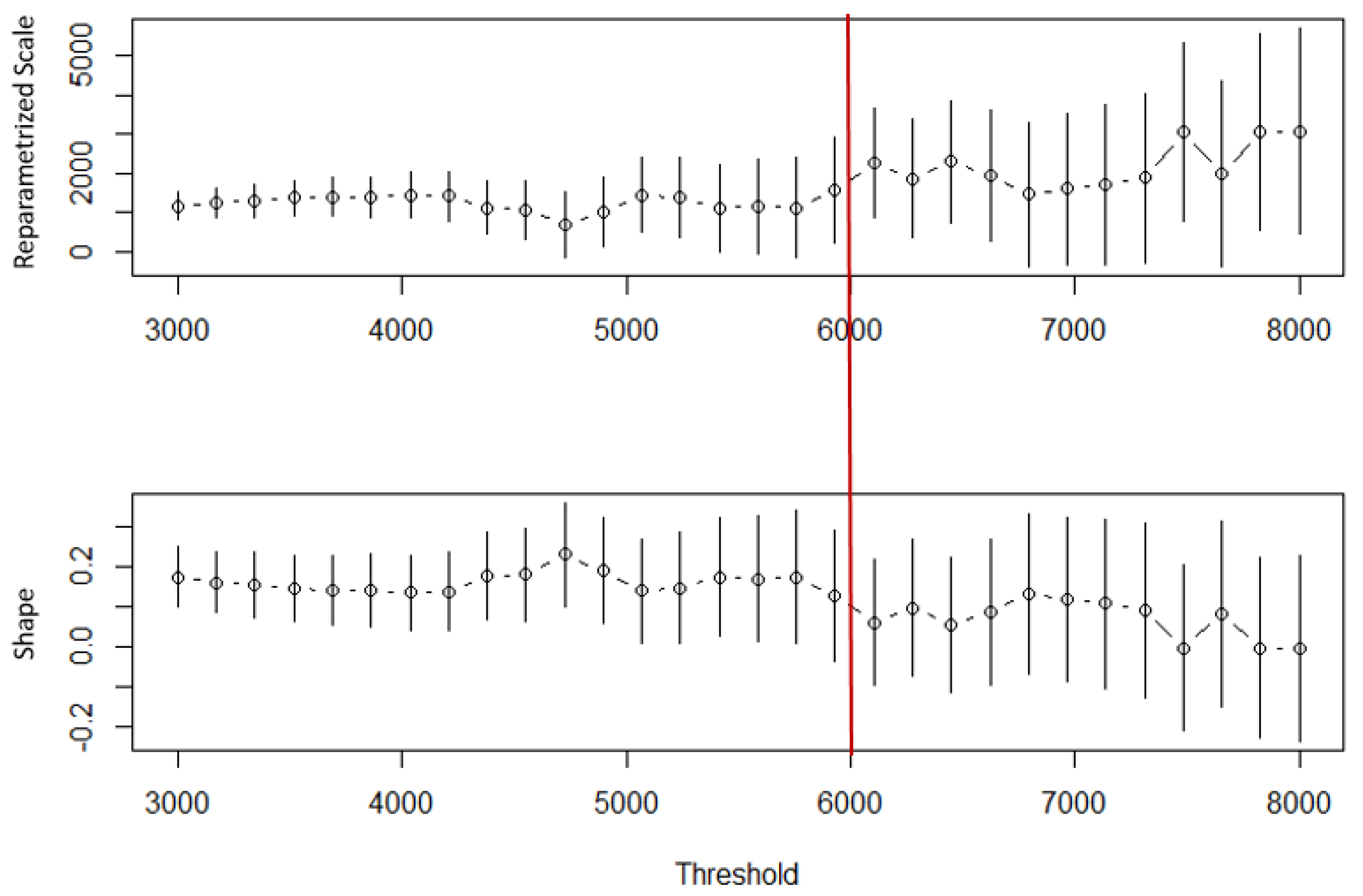
The implementation of GP in this study diagnosed an appropriate choice of threshold consistent with a Type II test. Two approaches in extRemes (R package) were used. threshrange.plot repeatedly fits the chosen distribution to the data for a sequence of threshold choices along with variability information. The plots created are subjectively interpreted to select a threshold that appears to yield stable estimates (within uncertainty bounds) as the threshold increases further, while remaining low enough as to utilize as much of the data as possible. Figure 2 shows the fitted scale and shape parameters over a range of thirty equally-spaced thresholds from 3000 to 8000 cfs for a site in Georgia (NYSDOT failure database Bridge ID # 287, USGS Station ID 02208450). A subjective selection of 6000 cfs appears to yield estimates that maximize the stability of the POT distribution parameter estimates [18,49,50].

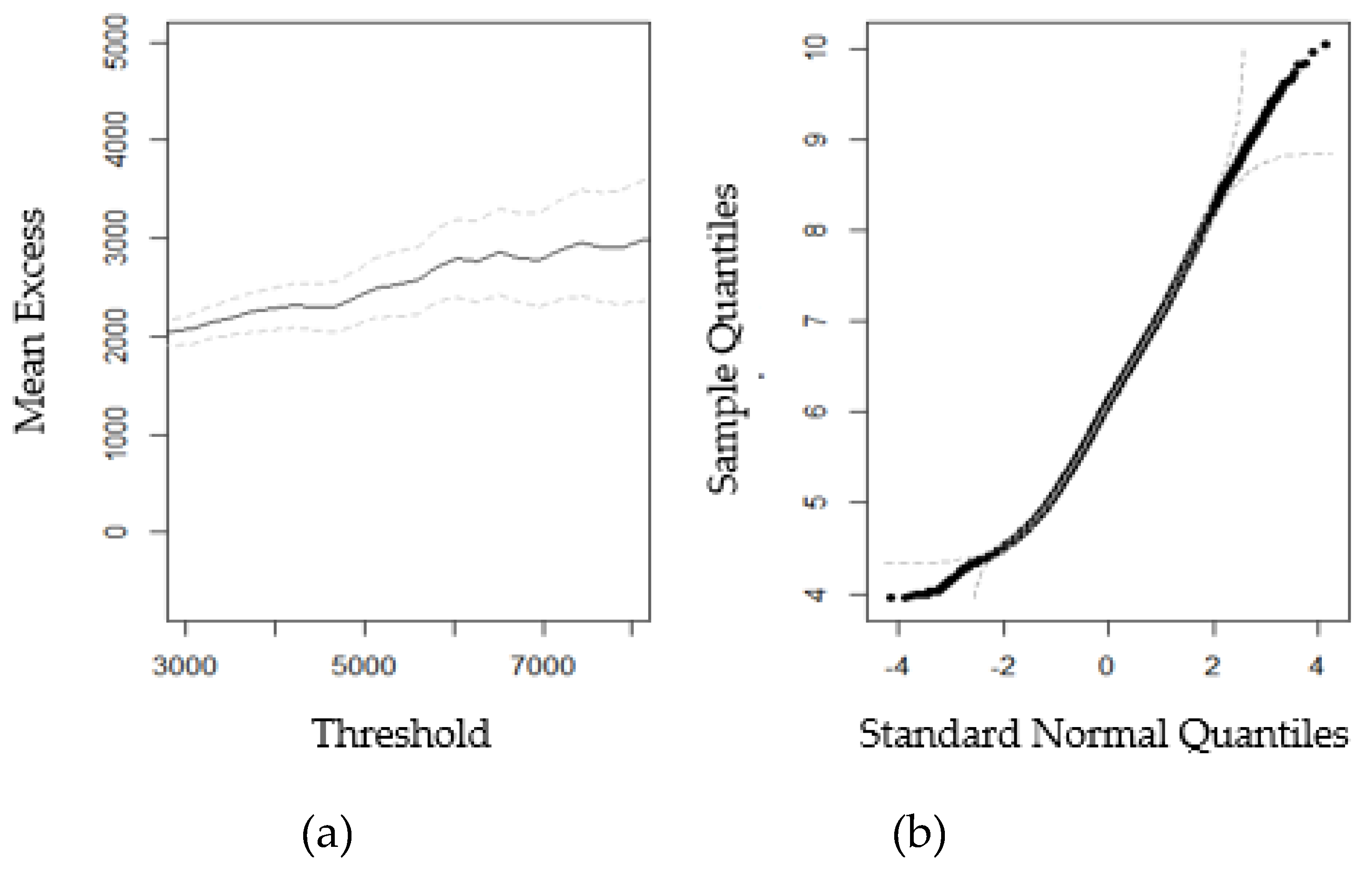
The second approach to threshold selection is implemented in mrlplot, which plots the mean excess values for a range of threshold choices [24]. The plot is used to select a threshold whereby the graph is linear, again within uncertainty bounds, as the threshold increases (Figure 3). Again, 6000 cfs appears to be a reasonable choice for the threshold as a reasonably straight line could be placed within the uncertainty bounds from this point up (Figure 3). The mean excess above threshold linearly changes with the height of the threshold for a GP distribution (Figure 3) and is constant for an exponential distribution. The quantile plot in Figure 3 draws the correlation between sample and normal distribution and was used to check the normality of the data.

2.3.3. Poisson Process (PP)

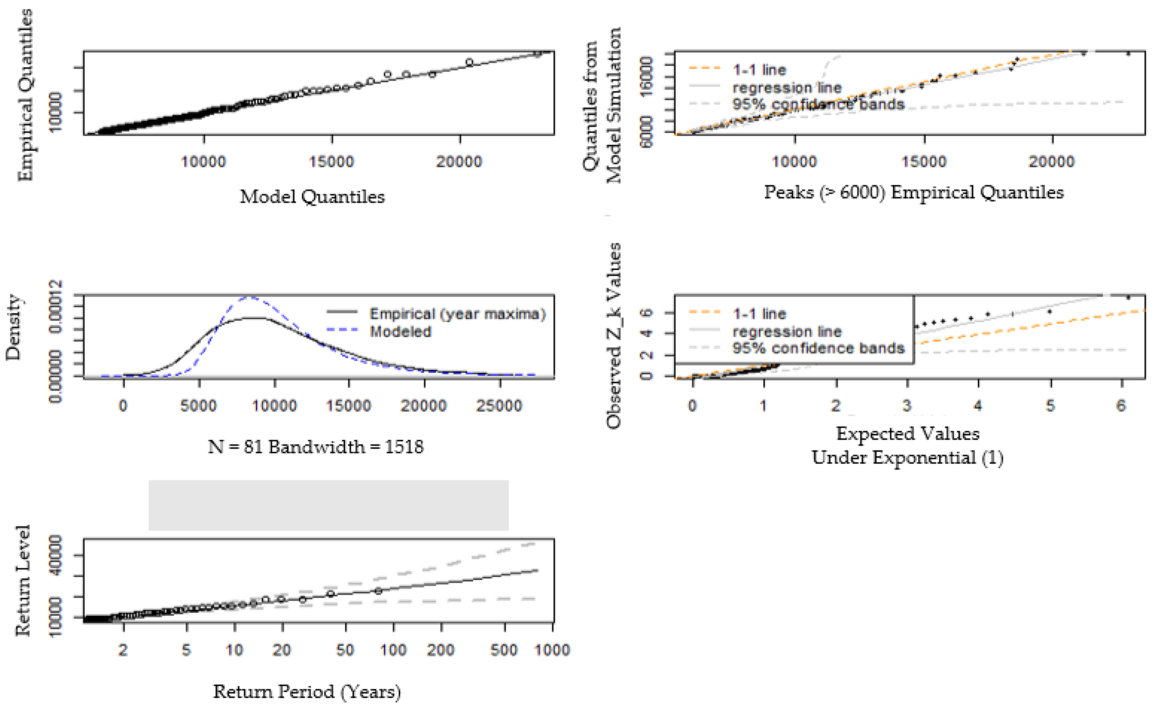
For fitting the PP distribution, three types of diagnostic plots [21] were used to evaluate the Poisson process distribution: quantile, density plot, and “Z” (Figure 4). The quantile plots check the validity of the corresponding GP distribution for only the data exceeding the threshold suitable for the Poison process. The density plot, on the other hand, shows the density for the equivalent GEV distribution. The Z plot is a quantile-quantile plot [44] and checks the underlying assumption of a Poison process, i.e., peaks over threshold should be independent and exponentially distributed in time. Figure 4 provides example diagnostic plots for the fit to the daily flow data for the same bridge collapse site in Georgia (NYSDOT failure database Bridge ID #287 Station ID 02208450). In Figure 4, all the fits appear reasonable except the Z plot. The Z plot suggests that the assumptions for the PP model are not met (infinite upper confidence level); for the present example, it turns out that while the threshold of 6000 cfs may be high enough to adequately model the threshold excesses, it may be too low to model the frequency of occurrence.

2.4. Calculating Return Periods

The quantiles of the GEV distribution are of particular interest because of their interpretation as return levels; the value expected to be exceeded on average once every 1/p period, where p is the specific probability associated with the quantile. The quantiles of the GP and PP distribution cannot be as readily interpreted as return levels because the data no longer derives from blocks of equal length. An estimate of the probability of exceeding the threshold (ζ_u) is required [21]. The peak flow value (x_m) that is exceeded on average once every m observation is estimated using the following equation [21]:

$$x_m=\{\begin{array}{c}u+\frac{{\sigma }_u}{\epsilon }\left[{\left(m{\mathsf{\zeta }}_u\right)}^{\epsilon }-1\right], \epsilon \ne 0,\\ u+{\sigma }_{u}ln\left(m{\mathsf{\zeta }}_u\right),\epsilon =0.\end{array}$$

(2)

Here u is the threshold, ${\sigma }_u$ is the scale parameter, and $\epsilon$ is the shape parameter.

3. Results

3.1. Analyzing GEV Parameters

GEV parameters were analyzed to check whether the collapse sites were consistent when regressed on the drainage area. In order to verify whether a scaling with drainage area is reasonable for the bridge collapse sites within a physiographic region, the scatter plot of the logarithm of the maximum likelihood estimates (MLE) of the GEV parameters (scale and location parameters) versus the logarithm of the drainage area was examined for a subset of 30 sites within Appalachian Highland region. Analysis of GEV parameters within each specific region was not performed because it was not possible to obtain an even distribution of bridges across different regions in the United States. There was a lack of comprehensiveness of the NYSDOT database (with the relative overrepresentation of Appalachian Highland) as well as the lack of a geographically uniform placement of stream gauges. The clustering of collapses in Appalachian Highland reflects not a higher rate of hydraulic collapses in this region but rather the limitation of data availability. In this study, 30 sites are located in the Appalachian Highland, 10 sites in the interior plains, 1 in Rocky Mountain, and 1 in the Atlantic plain. Due to the small number of sample sizes, analysis of GEV parameters was not performed for the interior plains, Rocky Mountain, and the Atlantic plain.

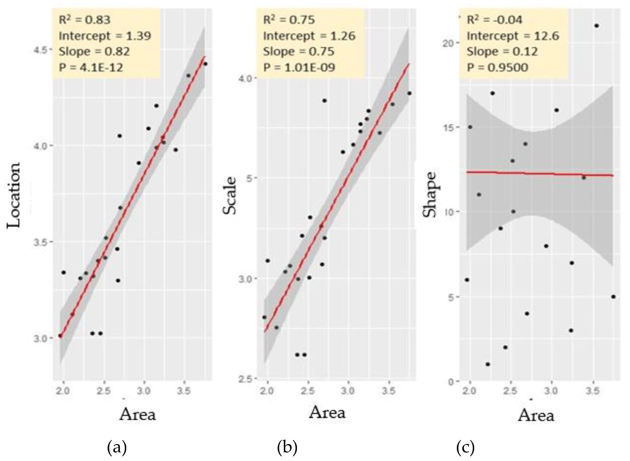
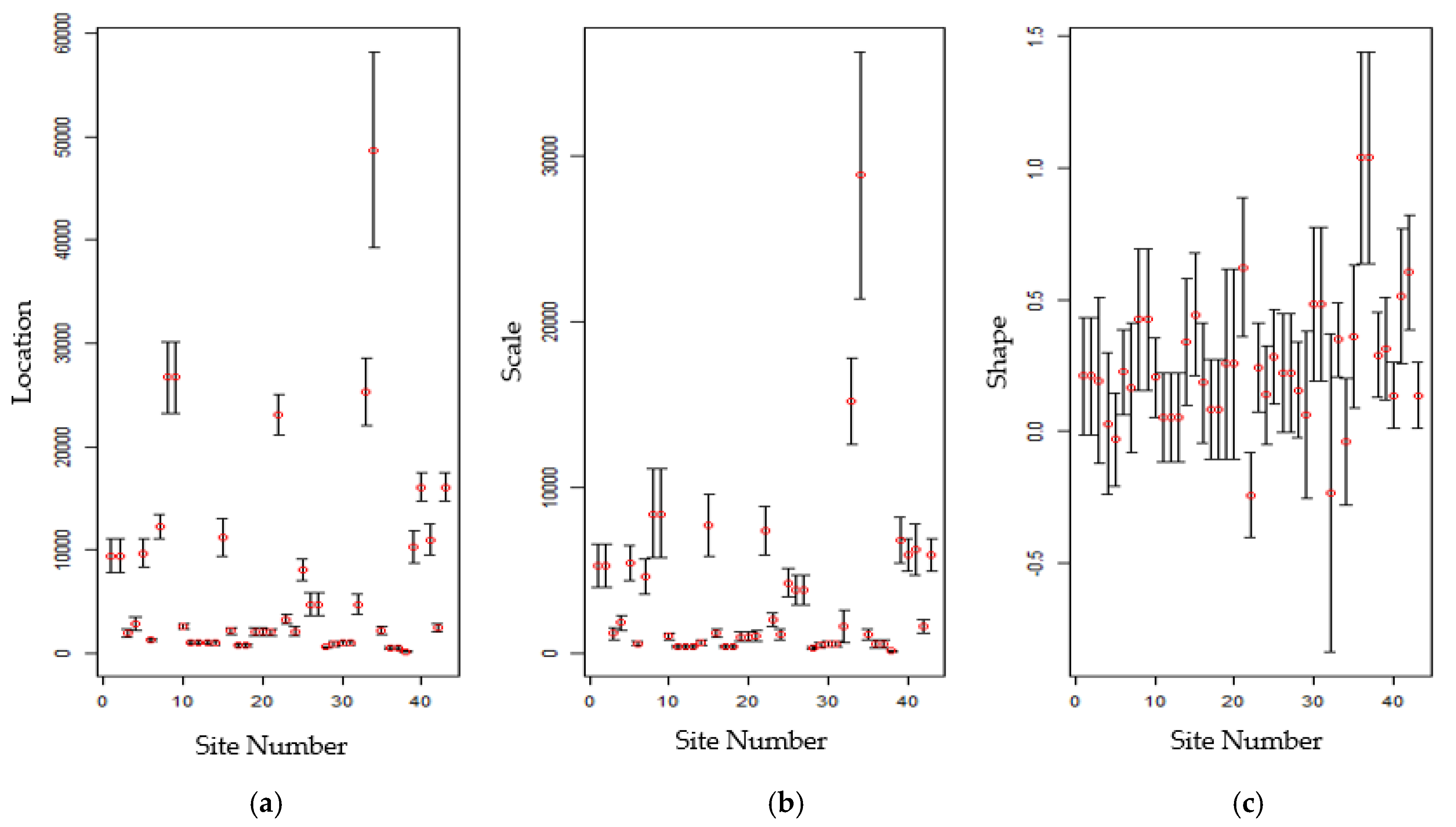
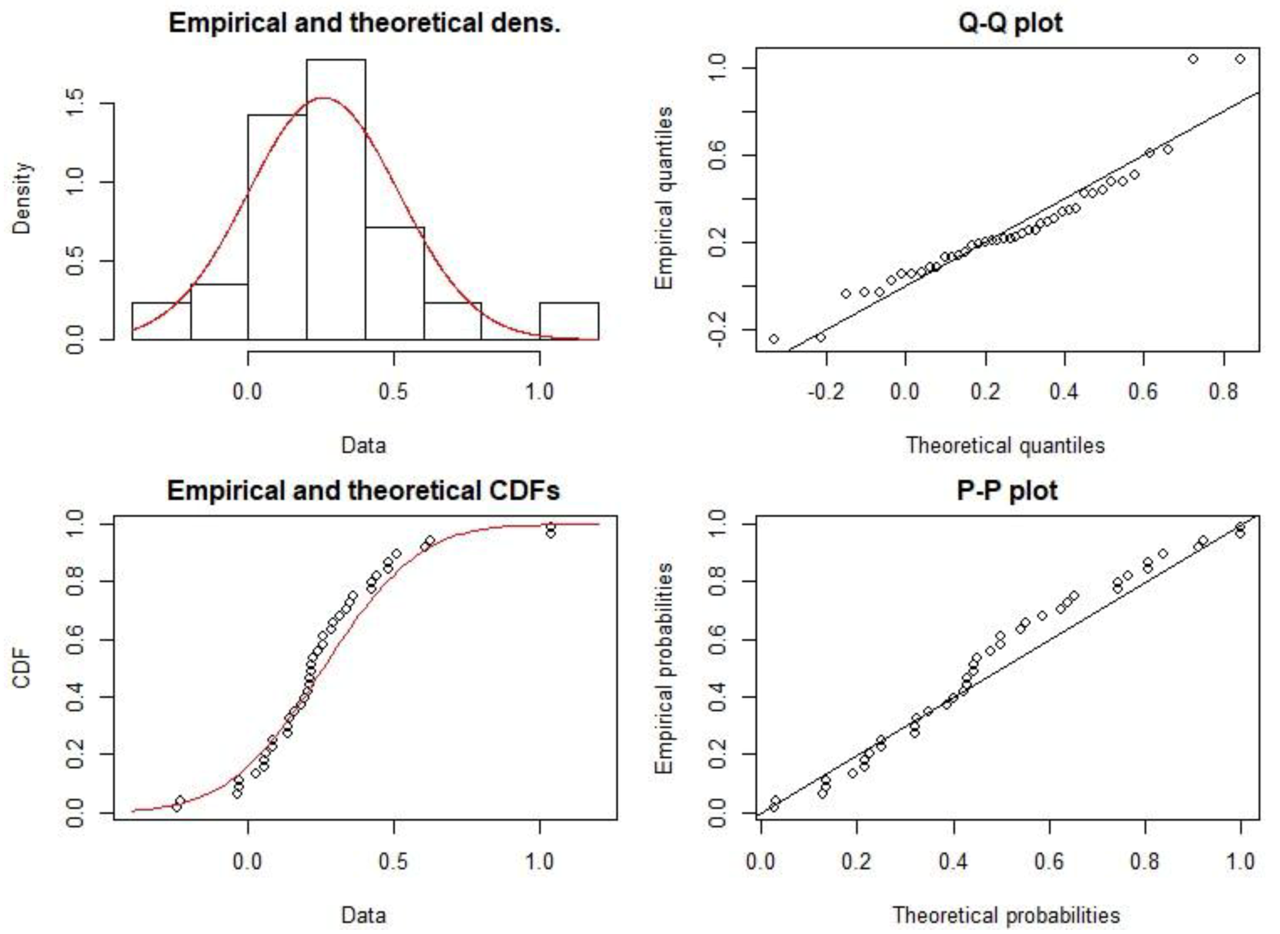
For the Appalachian Highland, as shown in Figure 5, both location and scale parameters present a well-defined log–log linear relationship with the drainage area. In line with expectations, the drainage area regression results for the shape parameter do not present strong evidence of a relationship, as shown in Figure 5. This result agrees with recent studies [29,30,32,33,37,43] which also suggest a poor relationship between the shape parameter and basin area based on the finding that the shape parameter mostly depends on climate indices. The shape estimates also exhibit a strong degree of pooling; 37 out of 42 collapse sites have a heavy tail distribution (shape parameter >0) (Figure 6). The shape parameter is modelled by a normal distribution (Figure 7) with a common mean across all sites in different physiographic regions.

3.2. Analyzing GEV Flood Index Values

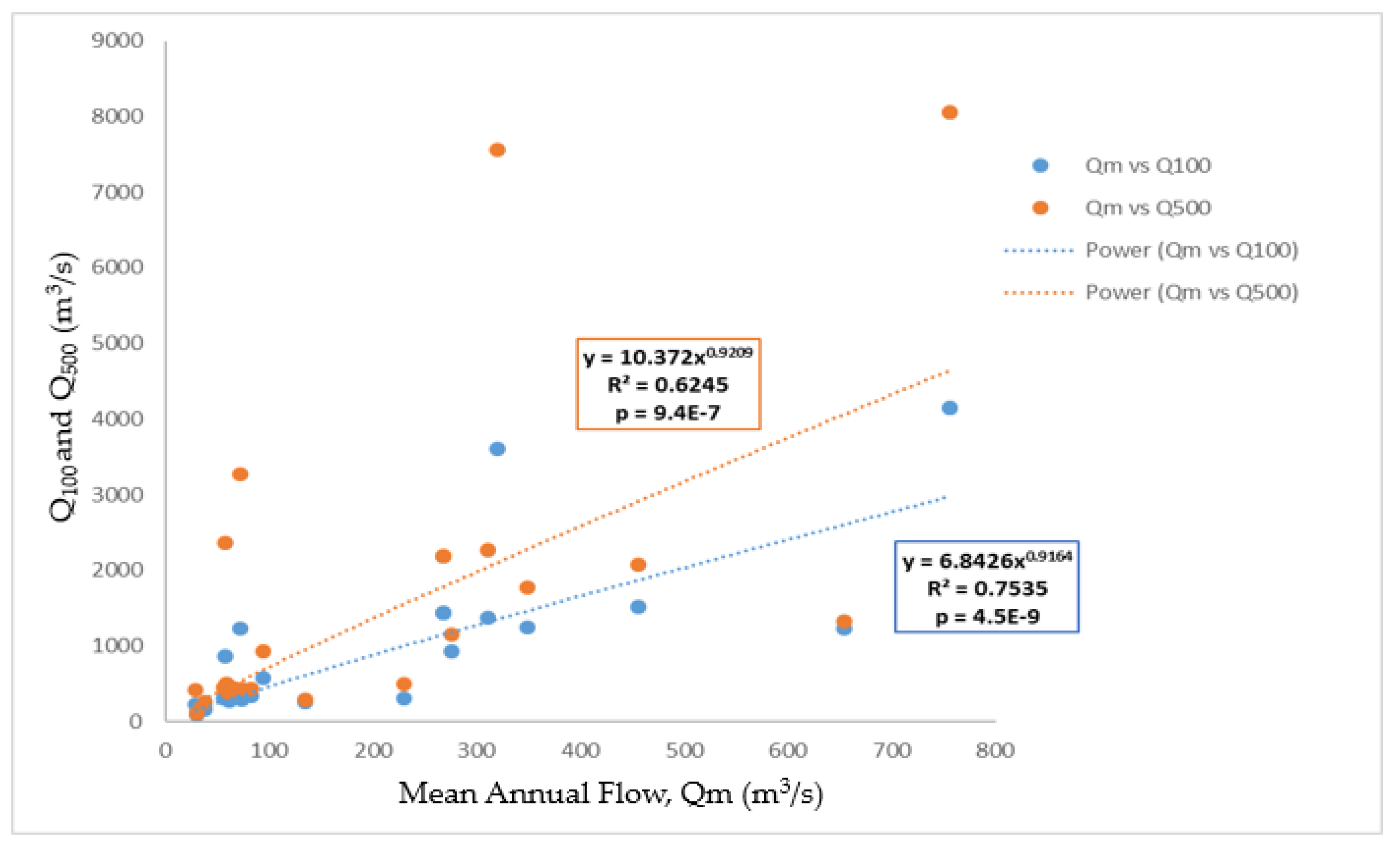
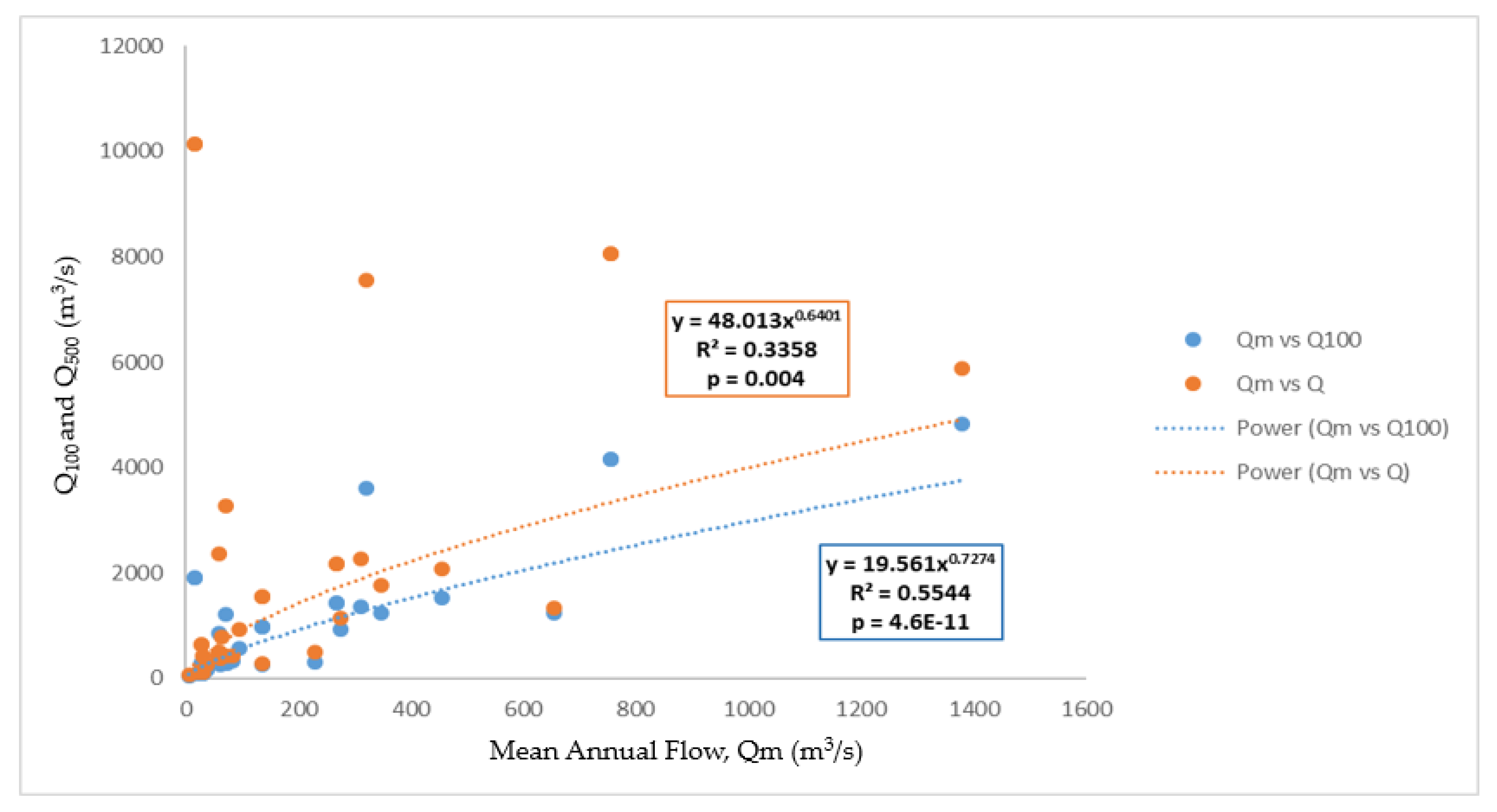
For the homogeneous regions, based on the concept of index flood method, a power relationship can be expected between the mean annual flow and the flood quantile, with an exponent value equal to 1 [51]. This is because all flood frequency curves in a homogeneous region are scaled by the mean annual flow to produce one characteristic regional curve [51]. For the collapse sites, flood index values are calculated (

Table 2. Flood quantile estimation using annual peak flows fitted with GEV distribution.

NYSDOT Database Bridge ID/State	USGS Station (Sample Size Is Given in Superscript)	Distance to Gauge (km)	Basin Area (km2)	Length of Peak Flow Data (Years)	Mean Annual Flow (m3/s)	Q100 (m3/s)	Q500 (m3/s)	Flood Index for 100-Year Flow	Flood Index for 500-Year Flow
50/WV	0161150095	3.20	1,749,990.2	95	291.6	2272.6	3973.0	7.8	13.6
57/WV	0318250088	22.22	1398.59	88	455.9	1520.1	2079.7	3.3	4.6
118/NJ	0146585051	7.69	167.05	51	17.8	82.8	119.1	4.65	6.69
195/VA	0162480030	6.68	189.069	30	61.2	271.1	382.7	4.43	6.25
246/NY	0421350077	9.05	1129.23	77	348.2	1249.9	1766.3	3.59	5.07
283/GA	0221830051	13.80	2434.59	51	268.1	1429.5	2185.0	5.33	8.15
285/GA	0221830051	11.46	2434.59	51	268.1	1429.5	2185.0	5.33	8.15
287/GA	0220845045	8.68	468.788	45	56.2	302	454	5.37	8.08
288/GA	0221900045	12.89	455.838	45	81.8	335	432	4.10	5.28
456/MD	0164350068	7.41	162.65	68	57.9	869.1	2358.8	15.01	40.74
462/ME	0101000067	25.15	3473.17	67	654.7	1234.8	1326.4	1.89	2.03
811/NY	0609170041	18.83	229.21	66	30	91.3	116.6	3.04	3.89
812/NY	0610800063	96.01	284.90	66	30	91.3	116.6	3.04	3.89
825/NY	0609320044	14.05	229.21	66	30	91.3	116.6	3.04	3.89
826/NY	0609320044	9.03	91.17	77	28.9	230.4	416.4	7.97	14.41
829/NY	0610800063	32.93	5599.55	32	756.0	4151.7	8049.4	5.49	10.65
830/NY	0606150077	8.07	5599.55	32	756.0	4151.7	8049.4	5.49	10.65
864/NY	0423900066	13.75	326.34	92	73.6	292.3	432.6	3.97	5.88
992/SC	0424001066	17.56	1411.54	74	275.2	933	1143	3.39	4.15
1482/MD	0423900066	4.44	127.17	69	37.3	167.2	255.2	4.48	6.84
1484/MD	0423300077	2.61	499.87	13	134.7	261.8	282.6	1.94	2.10
1547/ME	0153033232	21.13	233.10	47	59.4	305.9	487.7	5.15	8.21
1548/ME	0153033232	21.13	233.10	47	59.4	305.9	487.7	5.15	8.21
1630/NY	0423400092	2.84	497.28	86	320	3610.2	7563.3	11.28	23.64
3619/NY	0421650086	5.22	99.20	81	61.7	312.2	463.5	5.06	7.51
1044/VA	0421650086	1.86	852.11	89	229.3	305.9	487.7	1.33	2.13
1164/WV	0219600074	19.34	1686.08	91	311.4	1368.5	2273.6	4.39	7.30
1168/WV	0202150089	6.33	266.77	76	71.4	1227.7	3264.8	17.2	45.7
1177/WV	0160650091	8.51	1398.6	96	455.9	1520.1	2079.7	3.3	4.56
1251/VA	0160750076	13.04	334.11	89	93.7	576.8	920.8	6.16	9.83
503/MT 2	0318250090	22.22	647.50	41	63.7	435	794.6	6.8	12.5
506/MT 2	0206850089	8.40	3206.41	63	14.6	1899	10,148.4	130	695
512/MT 2	0158509023	0.50	396.27	44	28.4	294.7	645.3	10.38	22.72
513/MT 2	0689235044	5.83	396.27	44	28.4	294.7	645.3	10.38	22.72
901/NY 2	0688800061	14.98	57.24	86	23.5	88.8	118.3	3.78	5.03
904/NY 2	0688850065	12.14	57.24	86	23.5	88.8	118.3	3.78	5.03
515/MT 2	0159650069	2.49	3206.41	63	14.6	1899	10148.4	130	695.1
1450/KS 2	0161352513	6.56	154,767.33	44	1379	4821.5	5888.7	3.50	4.27
1455/KS 2	0104600047	3.21	629.37	61	135.3	989.0	1559.4	7.31	11.53
1464/KS 2	0104600047	1.49	629.37	65	135.3	989.0	1559.4	7.31	11.53
524/MT 3	0136250086	1.87	497.28	77	5.9	36.8	61.9	6.2	10.5
1262/MD 4	0136500081	3.15	7.07	23	27	102.5	134.6	3.80	4.99

) and diagnostic plots of mean annual flow versus quantile flow (Figure 8 and Figure 9) are created to check the homogeneity of the collapse sites. As expected, within certain physiographic regions, i.e., the Appalachian Highland, a power correlation is detected between the mean annual flow and flood quantiles (Q100 and Q500) with an exponent value of 0.9 (close to 1) (Figure 8). When considering all collapse sites within different physiographic regions, the exponent value decreases to 0.7 and 0.6 for 100 and 500-year flood quantiles, respectively (Figure 9). Nonetheless, a poor positive correlation is detected between the mean annual flow and the flood quantiles (R² = 0.6, Figure 8; R² = 0.3, 0.5, Figure 9) except for the Q_Mean versus Q₁₀₀ relationship in the Appalachian Highland (R² = 0.75, Figure 8). These results for correlation are statistically significant (p < 0.05).

3.3. Peak Over Threshold Analysis

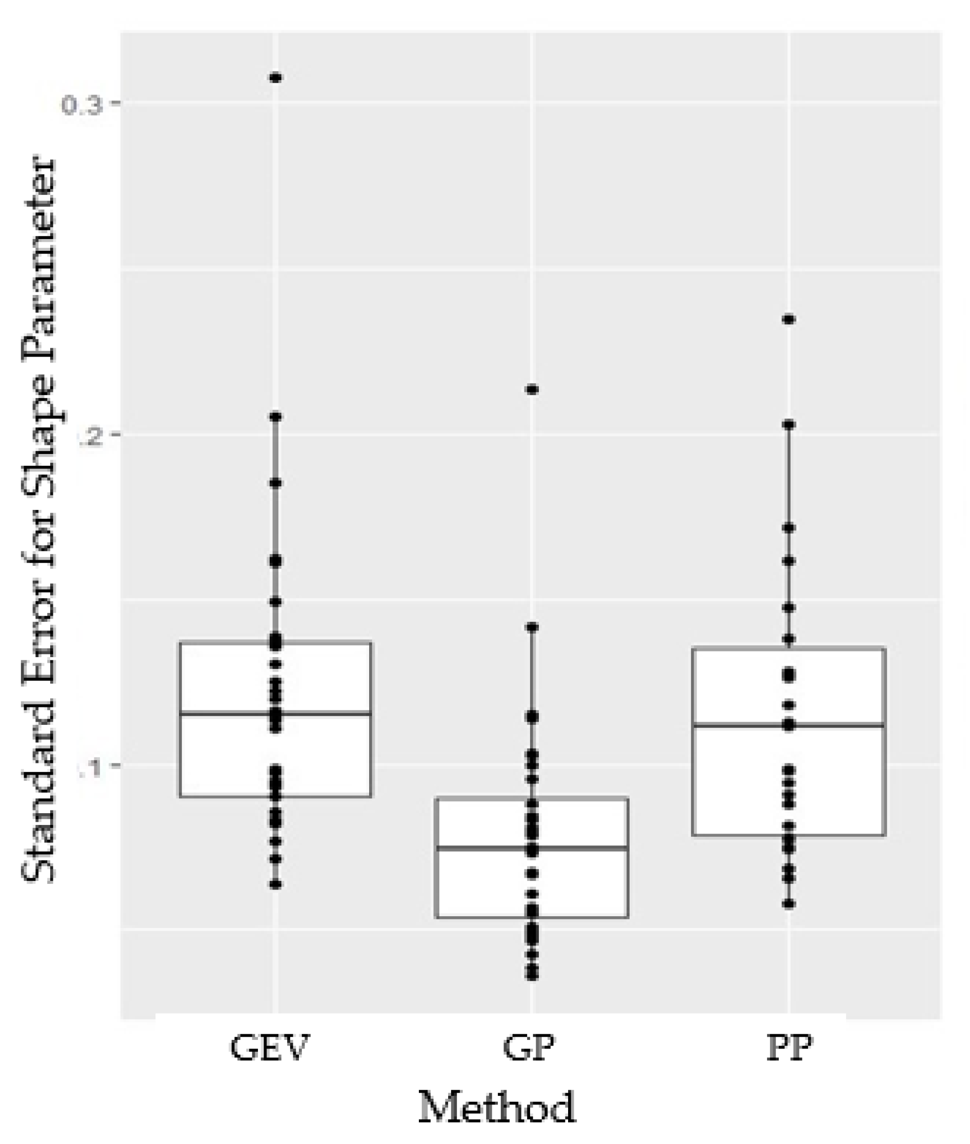
For peaks over threshold analysis, a comparison was made between GP and PP models. It was found that the threshold level had often to be raised significantly above the GP set in order to meet exponentially-based tests of the PP distribution (

Table 3. Peaks over threshold analysis using daily flow data retrieved from USGS.

NYSDOT Failure Database Bridge ID	Length of Daily Flow Data (Years)	GP			PP			Extremal Index
		Threshold	Average Number of Exceedances Per Year	AIC, BIC	Threshold	Average Number of Exceedances Per Year	AIC, BIC
50	95	3400	7.76	13,565.0, 13,574.3	5220	3.55	6196.4, 6208	0.33
57	90	×	×	×	×	×	×	×
118	32	250	11.31	7932.7, 7941.7	500	1.85	1479.8, 1487.8	0.18
195	30	310	8.45	3616.6, 3623.8	595	3.55	1505, 1513.1	0.35
246	8	6000	2.67	3857.4, 3864.2	8000	1.22	1942.8, 1950.6	0.64
283	42	8850	2.88	2254.7, 2260.3	×	×	×	0.27
285	42	8850	2.88	2254.7, 2260.3	×	×	×	0.27
287	5	1200	5.90	4347.8, 4355.1	3000	0.63	567, 570.3	0.3
288	48	1350	3.93	4697.8, 4705.2	1839	2.30	2460.1, 2469.1	0.3
456	63	670	2.14	2220.8, 2226.9	670	2.14	2296.6, 2305.7	0.56
462	69	17,500	5.73	7671.8, 7679.8	19,900	3.59	4665.9, 4676.4	0.24
503	40	1490	14.65	9411.9, 9420.8	×	×	×	0.10
506	64	370	19.67	18,288.1, 18,298.4	×	×	×	0.05
512	45	1500	1.04	718.7, 722.5	×	×	×	0.33
513	45	1500	1.04	718.7, 722.5	×	×	×	0.34
515	64	370	19.67	18,288.1, 18,298.4	×	×	×	0.05
524	78	×	×	×	×	×	×	×
811	68	850	2.77	2353.2, 2359.8	1100	0.57	615.9, 620.9	0.41
812	49	790	3.90	3317.6, 3324.8	805.3	3.61	2926.3, 2936.8	0.36
825	68	790	3.90	3317.6, 3324.8	1000	1.07	1061, 1067.9	0.36
826	75	390	2	1991.8, 1997.8	390	2	2087.1, 2096.2	0.52
829	9	6900	25.36	5253.7, 5260.9	16,048	3.27	654, 658.70	0.17
830	9	6900	25.36	5253.7, 5260.9	16,048	3.27	654, 658.70	0.17
864	94	1370	3.62	5146.5, 5154.2	2500	0.61	1083.3, 1089.4	0.63
901	72	390	1.16	1573.8, 1579.5	500	0.60	1033.4, 1040	0.75
904	72	390	1.16	1573.8, 1579.5	500	0.60	1033.4, 1040	0.75
992	74	8200	1.66	2372.9, 2378.6	12,500	0.52	876.1, 881.6	0.46
1044	91	3900	3.08	4916.2, 4923.5	3900	3.08	876., 881.6	0.60
1164	91	2900	10.97	2296.6, 2305.7	×	×	×	0.28
1168	76	790	7.18	17,790.2, 17,800	5220	3.78	4665.9, 4676.4	0.44
1177	90	×	×	×	×	×	×	×
1251	78	620	6.5	1505, 1513.1	×	×	×	0.35
1262	23	43	6.4	9004.242, 9013.114	878	3.427083	4848, 4859.2	0.76
1450	102	40,200	8.1	1448.1, 1454.2	×	×	×	0.13
1455	45	750	3.96	18,184, 18,193.5	1500	1	2841.2, 2850.5	0.31
1464	65	750	3.96	5401.8, 5409.5	1500	1.95	1479.8, 1487.8	0.31
1482	7	641.08	4.0	3686, 3692.3	750	1	2290.8, 2300.2	0.18
1484	13	1500	5.6	3434.4, 3441.5	×	×	×	0.47
1547	49	1500	2.0	2521.5, 2527.8	2300	1	876.1, 881.6	0.43
1548	49	1500	1.89	2521.5, 2527.8	2300	0.53	876.1, 881.6	0.43
1630	87	3250	5.34	2521.5, 2527.8	3850	0.53	5489.6, 5500.9	0.54
3619	81	780	2.71	8258.3, 8266.7	780	3.58	3186.2, 3196.5	0.62

). Whereas it is important to choose a sufficiently high threshold in order that the theoretical justification applies, thereby reducing bias, a higher threshold also implies that fewer available data remain. The uncertainty in the estimation of distribution parameters becomes greater as the threshold increases and the sample size decreases [51]. The comparatively higher standard error in shape parameter estimates for PP models can be attributed to the fewer data remaining above the threshold (Figure 10).

3.4. Comparing GEV, GP, and PP

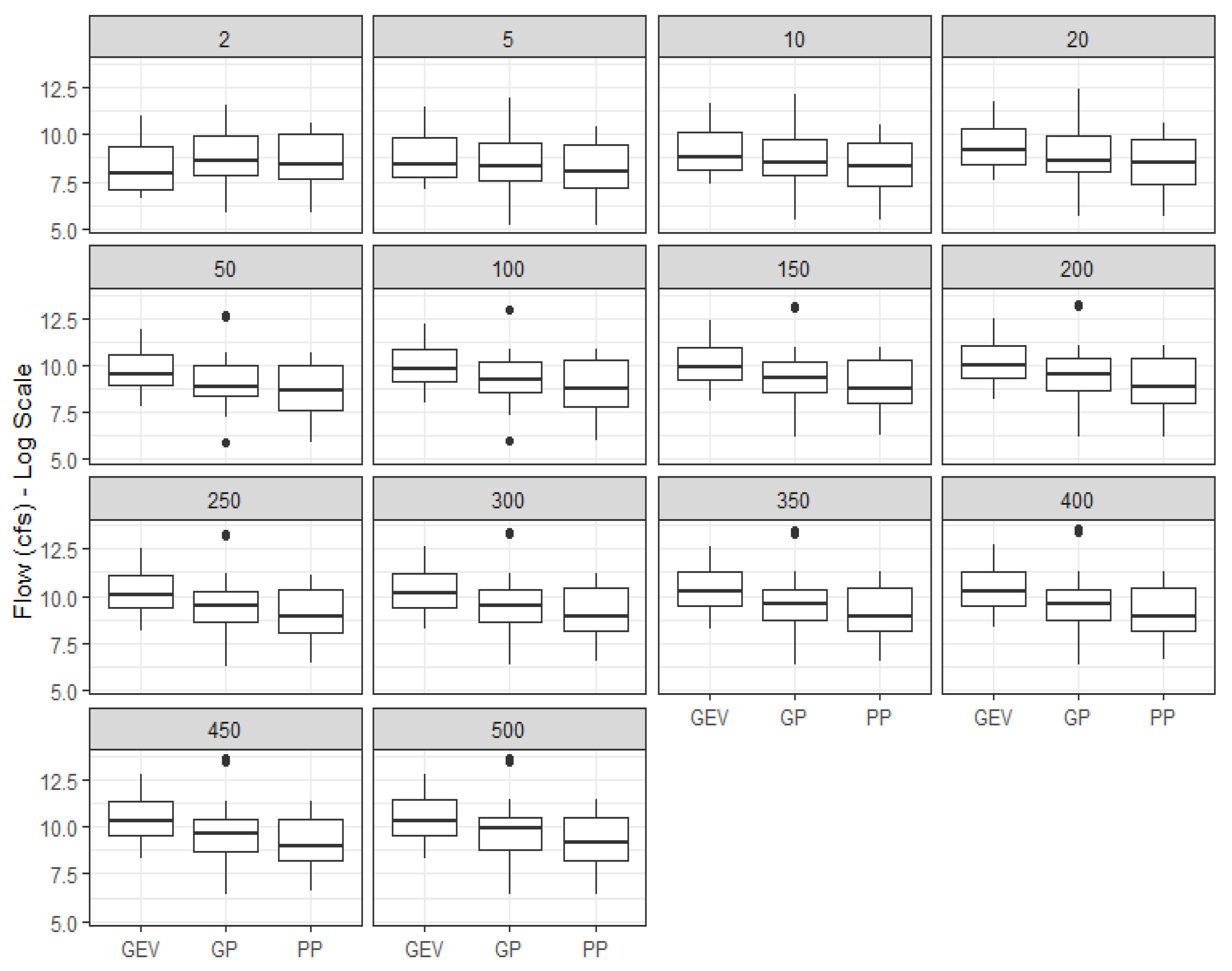
Comparing GEV, GP, and PP models (Figure 11), certain comments can be made:

• GEV predicts a higher median flow as compared to GP and PP (for return period ≥50 years).
• GP overestimates flow as compared to PP (particularly for return period ≥100 years). For instance, for a site in NY (Failure database ID 811) the 50-year flow is about 2861, 1666, and 1639 cfs for GEV, GP, and PP models, respectively.
• For all larger flood events (for return period ≥50 years), an outlier is identified in GP models, implying that an extremely high flood event can be expected for a return period higher than 50 years. GEV and PP models do not identify any outliers.
• The confidence interval is larger for the PP model as compared to GP and GEV models, indicating greater uncertainty when using the PP approach.

3.5. Calculating Return Periods for Maximum Flows in Collapse Year Using GEV, GP, and PP

The return periods of maximum flows in the collapse year obtained using different types of flow data (maximum daily mean flow, maximum peak flow) are quantified in

Table 4. Calculated return periods using daily mean and annual peakflow values (maximum in collapse year).

NYSDOT Database Bridge ID/State	USGS Station ID	Built-Collapse Year	Maximum Flow (m3/s) in Collapse Year		Return Period, T (Year)
			Daily Mean Fitted with GP and PP	Peak Fitted with GEV	T for Daily Mean (Max)			T for Annual Peak
					GP	PP	GEV	GP	PP	GEV
50/WV 1	01611500	–1996	206.43		4.5	2.1	1.24
57/WV 1	03182500	–1996	1124.18	1741.49			25.1			197
118/NJ 1	01465850	1931–2004	98.26	117.80 A	4313.2	4183.2	208.3	8450.7	784.5	474.7
195 */VA 1	01624800	1935–1996	129.97	458.73	618.95	269.67	6.9	78,593	33,598.5	1257
246 */NY 1	04213500	1983–2009	521.03	920.30	62.56	30.67	3.8	1855.0	3180.7	27.3
283/GA 1	02218300	–1990	583.33	897.64	70.9		6.2	90,027,071		20.8
285/GA 1	02218300	–1990	583.33	897.64	70.9		6.2	90,027,071		20.8
287 */GA 1	02208450	–1990	183.21	215.77	240.2	88.4	18	564.7	1637.4	30.5
288 */GA 1	02219000	–1990	174.71	NA	156.1	92.6	6.3
456/MD 1	01643500	1928–	NA	NA
462 */ME 1	01010000	1935–1959	455.90	461.56	1	1	1.1	1	1	1.1
503/MT 2	06091700	1949–1964	NA	NA
506/MT 2	06108000	1919–1964	566.34	2018.99	4611.8		31.6	109,244		106
512/MT 2	06093200	1924–1964	NA	NA
513/MT 2	06093200	1924–1964	NA	NA
515/MT 2	06108000	1936–1965	48.99	56.63	4611.8		31.6	109,244		106
524/MT 3	06061500	1934–1981	54.65	65.13			337.3			588.5
811 */NY 1	04239000	1913–1920	NA	NA
812 */NY 1	04240010	1915–1920	NA	NA
825 */NY 1	04239000	1915–1972	42.76	90.61 B	73.4	19	3.4	68,349,243	inf	95.3
826/NY 1	04233000	–1972	47.86	135.92 C	80.9	82.9	3	23,179.7	26,595.9	25.9
829/NY 1	01530332	–1972	NA	6654.46 C				inf	inf	315.8
830/NY 1	01530332	–1972	NA	6654.46 C				inf	inf	315.8
864/NY 1	04234000	1920–1981	199.92	68.53	392	132.6	23.7	5.34	1	1.4
901 */NY 2	04216500	1950–1989	NA	82.12				14,092.8	993,412.7	1.9
904 */NY 2	04216500	1934–1989	NA	82.12				14,092.8	993,412.7	1.9
992 */SC 1	02196000	1975–1977	255.42	504.04	1.26	1	1.5	11.96	3.4	5.1
1044/VA 1	02021500	–1985	1175.15	199.92	1531.3	1515.1	62.9	4.7	4.7	1.4
1164/WV 1	01606500	–1985	2180.40	356.79	9452.2		38.1	34.25		1.8
1168/WV 1	01607500	–1985	212.38	53.80 D	725.3	6.5	6.2	7.3	1	1.3
1177/WV 1	03182500	–1985	1257.27	322.81			25.1			197
1251/VA 1	02068500	1977–1992	127.14	348.30 E	91.9		2.3	1438.4		21.0
1262 */MD 4	01585090	–1971	NA	NA
1450 */KS 2	06892350	1904–1951	13,760.99	NA	1417.6
1455/KS 2	06888000	–1951	NA	750.40 F				1513.92	1098.6	41.3
1464/KS 2	06888500	1882–1951	NA	750.40 F				1513.92	1098.6	41.3
1482/MD 1	01596500	1940–1996	56.63	187.46	67.9	45.1	3.41	65,093.7	56,049.8	152.9
1484 *MD 1	01613525	1950–1996	NA	NA
1547 */ME 1	01046000	1957–1987	NA	NA
1548 */ME 1	01046000	1957–1987	NA	NA
1630/NY 1	01362500	1976–2005	492.71	1563.09 E	52.9	41.3	2.5	960.96	1126.1	17.7
3619 */NY 1	01365000	1956–2011	102.22	232.20 C	204.2	218.9	3.4	22,292.9	29,187.9	33.8

^A Dam failure. ^B Regulation, snowmelt, hurricane, debris jam. ^C Snowmelt, hurricane, ice-jam, debris jam. ^D Regulation. ^E Regulation/diversion. ^F Historical peak. ¹ Appalachian Highland (30 sites). ² Interior plains (10 sites). ³ Rocky Mountain (1 site). ⁴ Atlantic plain (1 site). * Fail to reject Gumbel distribution. Unprecedented event (extremely high flow). Return period cannot be calculated because of the unavailability of data or invalidity of peak over threshold analysis.

. For some of the sites, the return period cannot be calculated because of the unavailability of max flow data and/or inability to use peak over threshold analysis (due to the invalidity of the underlying assumption). Like the flow values, the collapse return periods varied considerably between the bridges, as evidenced by the range of the estimated values (daily mean: 1–9452 years; peaks: 1 to >90027071 years). These results are in accordance with the recent study on bridge collapse [52], where the authors also reasoned the relatively lower variability of daily mean as opposed to annual peak for a smaller number of very large return periods in the analysis using daily mean data. In the study, for daily mean data, the return period varies from 1 year to 9452.2 years; for annual peak data, the return period varies from 1 year to infinity.

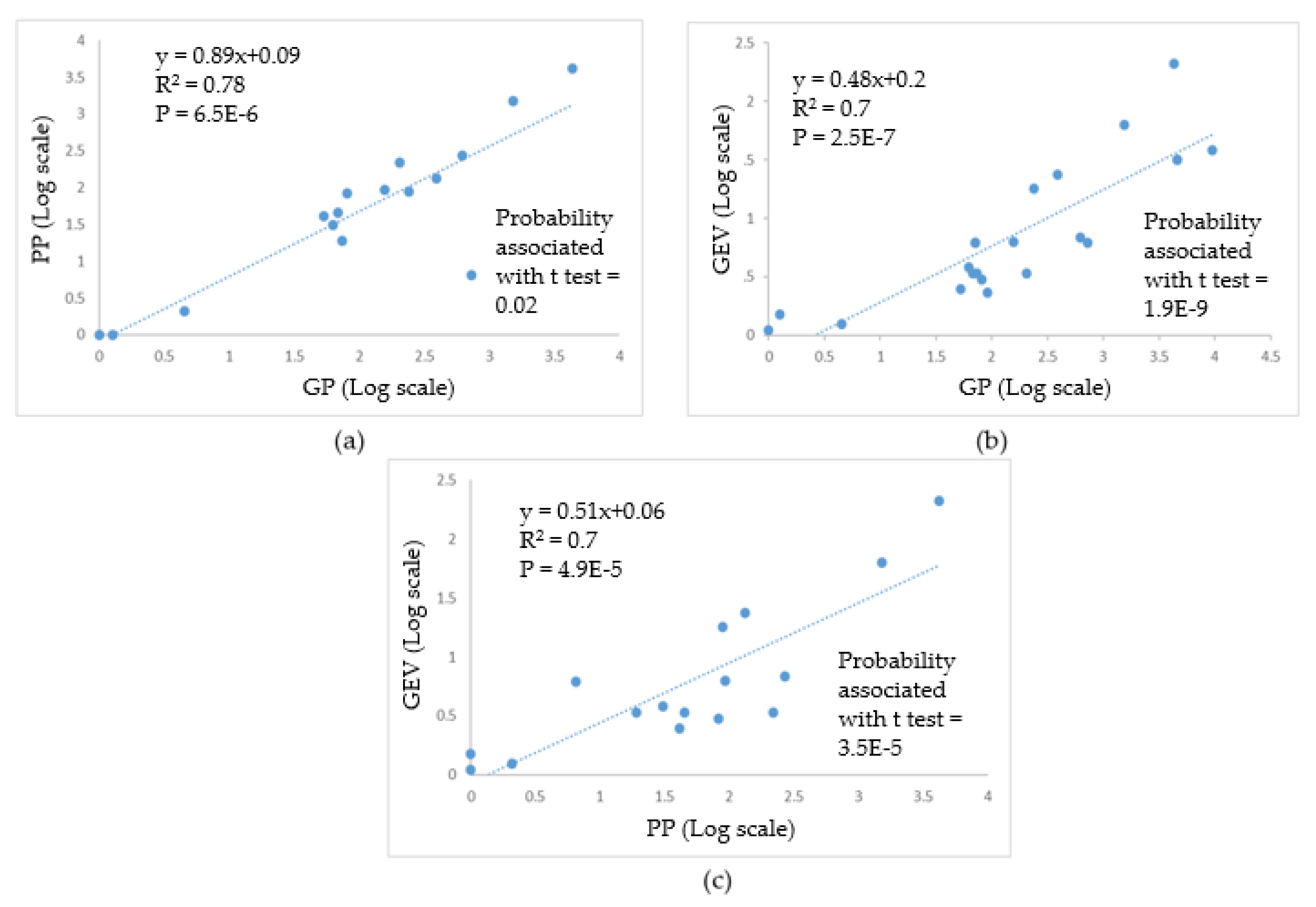
Plots highlighting the correlation between different estimates of max flow return periods (in collapse year) are provided in Figure 12 and Figure 13. A significant difference is identified between the max flow return periods estimated using daily mean flow values for all comparisons (GP versus PP, GP versus GEV, PP versus GEV) since probability associated with the t-test <0.05; nonetheless, statistically significant positive correlation is detected as p < 0.05, R² = 0.7 (Figure 12a–c).

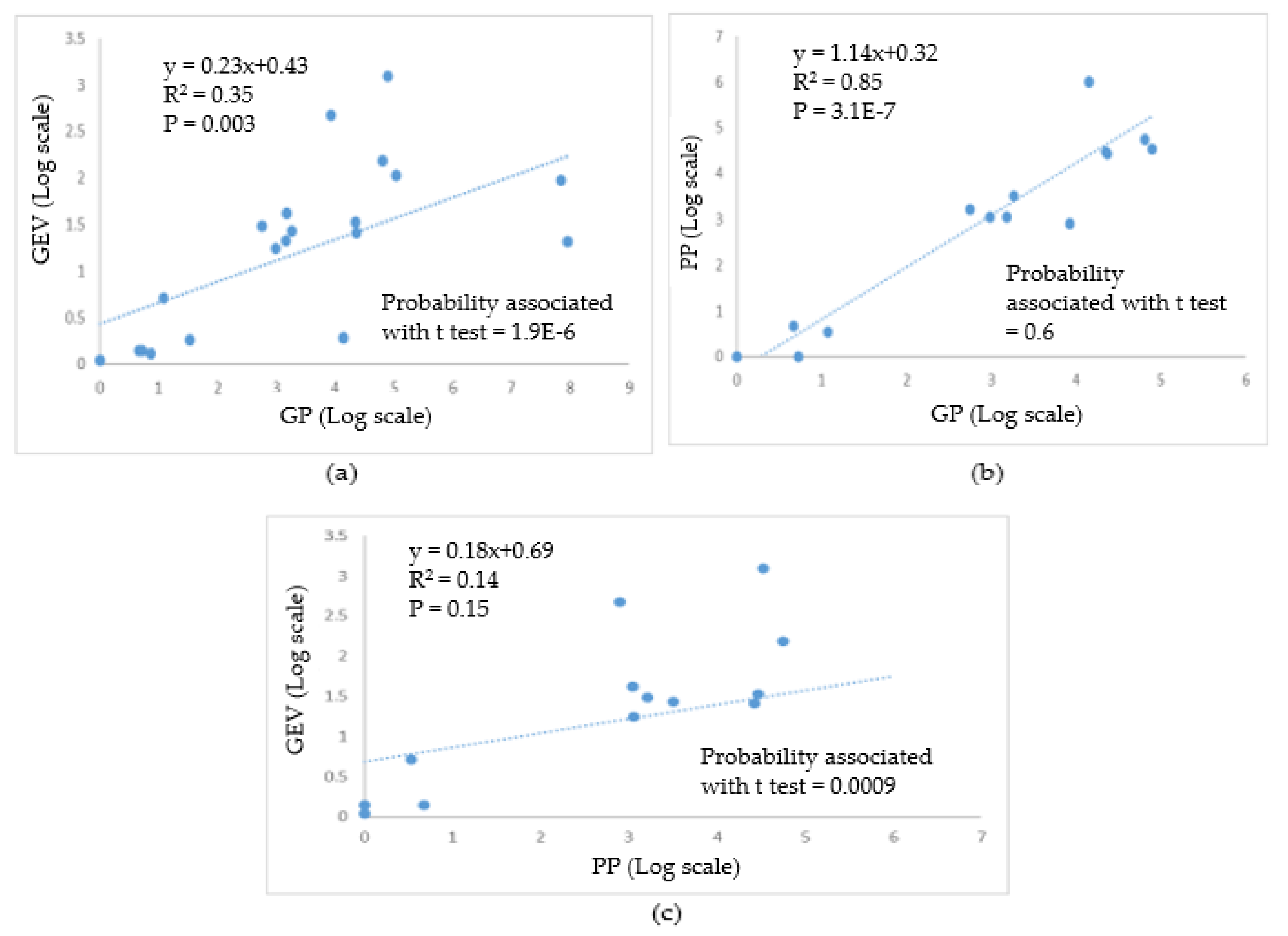
For the max flow return periods estimated using peak flows, significant difference is also identified for two comparisons as probability associated with the t-test <0.05 (GP versus GEV, PP versus GEV; Figure 13). No statistically significant difference exists for GP versus PP estimates using the peak flow values (probability associated with the t-test = 0.6; Figure 13). Poor correlation is detected for the GP versus GEV (p < 0.05, R² = 0.3), and PP versus GEV (p = 0.15, R² = 0.14) comparisons (Figure 13).

In summary, GEV, GP, and PP mostly produced substantially different return periods for both annual peak and daily mean flow values. For the study sites, a non-significant difference was only detected for the GP versus PP estimates using peak flows. The poor correlation was also found for GP versus GEV and PP versus GEV estimates using peak flows. These findings give cause for concern in implementing only one analysis using peak flow data in determining the collapse-inducing flows and/or design flows.

4. Discussion

4.1. Heavy Tail Distribution

Having a heavy tail distribution for the shape parameter is of critical significance for bridge hydraulics. Extreme values with heavy tail distribution follow catastrophe and/or Pareto principles (the principle of a single big jump) [53]. In river hydraulics, it implies that when sites with heavy tails exhibit big flows, it will be way bigger; in other words, outliers are expected and are not random. Another striking feature of heavy tails is that single big flow is expected at sites that are mostly exhibiting relatively low flows, which might convince the bridge engineers to ignore the outliers in a flood frequency analysis. Having a common mean for shape parameters with normal distribution across different physiographic regions (the Appalachian Highland, interior plains, the Atlantic plain) indicates a commonality in flood behavior (i.e., heavy tail or extremeness), for the collapse dataset studied. Well-defined scaling of location and scale parameters with drainage areas provides some basis for extending the findings obtained for the 30 collapsed bridges in other sites to assess risk of future collapses in the Appalachian Highland.

4.2. GEV, GP, PP

Based on the relatively lower values of AIC and BIC (defines best fit or not), GEV is apparently preferable over the GP and PP approaches for the bridge collapse sites studied. However, shape parameters (defining the behavior of floods) derived from GP are with comparatively lower standard error. GP was also able to identify the outliers, which might be of importance for sites with heavy tail distributions. The difficulty with using GP analysis, however, is that choosing a threshold might not possibly satisfy all the underlying assumptions of peak over threshold analysis, particularly for a poor dataset. It is, therefore, not possible to draw conclusions about which approach is best generally. Such a conclusion implies the decrepit approach of using only one flood frequency distribution when deciding the design flows of bridge structures.

4.3. Collapse Cause

Although the sample size is too small to retrieve any conclusive information regarding bridge collapse causes in US, some findings appeared to be robust:

• Maximum flow return periods in the collapse year were found to be in a significantly wide range. For some sites (#350, #462, #992) maximum flow return periods were calculated significantly lower based on available daily and annual peak flow data. It is possible that other hydraulic events may induce scour, accumulating over a long period of time even at low flows, resulting in total/partial bridge collapse. In fact, in the Appalachian Highland (a) debris jam causing increased flooding, (b) high erodible soil causing accelerated rate of channel widening, lateral migration and vertical degradation, and (c) high channel modification resulting in destabilized channels, led to accelerated scour even at low flows [54,55,56].
• For some sites (#118—dam failure, #825—regulation, snowmelt, hurricane, debris jam, #826, #829, ##830—snowmelt, hurricane, ice-jam, debris jam, #1455, #1464—historic peak), max flow return period in the collapse year coincides with the maximum recorded flow, which suggests that the bridges collapsed at unprecedent events at the sites. For these unprecedent events, annual peak flow data appear to be consistent with the recorded event by the United States Geological Survey (USGS). The calculated extremely high return periods (GP and PP estimates, 784.5 years to infinity) also indicate unprecedented events with no such previous record at these sites.

5. Conclusions

In this study, flood frequency analyses have been performed using peak flow data from 42 bridge collapse sites. For the sites in the study, a trend was derived in the flood magnitude (regressed over drainage area in the Appalachian Highland) and in flood behavior/extremeness (heavy tail distribution for most of the sites in different physiographic regions). Comparing the different approaches of flood frequency analysis, it is also derived that no single approach is generally best, considering its capability (only GP can identify outliers) and uncertainty (GEV is the best fit). Major findings that might have important implication in the risk study of bridge collapse include the following:

• The bridge collapse return period varies widely (very low to very high) although the apparent collapse cause is flood.
• Bridge collapses can be attributed to unprecedent events that could not have informed the bridge design.
• Bridge collapse due to scour can be expected even at low flows within the context of other hydraulic events, i.e., debris jam, ice-jam, high rate of channel migration, and destabilized channel due to channel modification.
• Channels with mostly low flows throughout the year can experience an unprecedent extreme flow. Such incidents are not a surprising event but rather expected for peak flows with heavy tail distributions.

References

- Cook, W.; Barr, P.J.; Halling, M.W. Bridge failure rate. J. Perform. Constr. Facil. 2015, 29. [Google Scholar] [CrossRef]
- Arneson, L.; Zevenbergen, L.; Lagasse, P.; Clopper, P. Evaluating Scour at Bridges, 5th ed.; HEC-18: FHWA-HIF-12-003; FHWA: Washington, DC, USA, 2012.
- Kattell, J.; Eriksson, M. Bridge Scour Evaluation: Screening, Analysis, & Countermeasures; USDA Forest Service: Washington, DC, USA, 1998.
- National Resources Conservation Service. Urban Hydrology for Small Watersheds; TR-55; USDA: Washington, DC, USA, 1986.
- Hydrology Subcommittee. Bulletin 17C Guidelines for Determining Flood Flow Frequency; USGS Interagency Advisory Committee on Water Data: Reston, VA, USA, 2019.
- Atkins, J.B.; Hummel, P.R.; Gray, M.; Dusenbury, R.; Jennings, M.E.; Kirby, W.H.; Riggs, H.C.; Sauer, V.B.; Thomas, W.O., Jr. The national streamflow statistics program: A computer program for estimating streamflow statistics for ungaged sites. In Hydrologic Analysis and Interpretation. Section A: Statistical Analysis; Ries, K.G., Ed.; USGS: Washington, DC, USA, 2007. [Google Scholar]
- Eljabri, S.S.M. New Statistical Models for Extreme Values. Ph.D. Thesis, The University of Manchester, Manchester, UK, 2013. [Google Scholar]
- Tyralis, H.; Papacharalampous, G.A.; Tantanee, S. How to explain and predict the shape parameter of the generalized extreme value distribution of streamflow extremes using a big dataset. J. Hydrol. 2019, 574, 628–645. [Google Scholar] [CrossRef]
- Lima, C.H.R.; Lall, U.; Troy, T.; Devineni, N. A hierarchical Bayesian GEV model for improving local and regional flood quantile estimates. J. Hydrol. 2016, 541, 816–823. [Google Scholar] [CrossRef]
- Morrison, J.E.; Smith, J.A. Stochastic modeling of flood peaks using the generalized extreme value distribution. Water Resour. Res. 2002, 38, 41-1–41-12. [Google Scholar] [CrossRef]
- Kuzuha, Y.; Tomosugi, K.; Kishii, T.; Komatsu, K. Coefficient of variation of annual flood peaks: Variability of flood peak and rainfall intensity. Hydrol. Process. 2009, 23, 546–558. [Google Scholar] [CrossRef]
- Veneziano, D.; Langousis, A. Scaling and fractals in hydrology. In Advances in Data-Based Approaches for Hydrologic Modeling and Forecasting; Sivakumar, B., Berndtsson, R., Eds.; World Scientific: Singapore, 2010. [Google Scholar] [CrossRef]
- Blöschl, G.; Sivapalan, M. Process controls on regional flood frequency: Coefficient of variation and basin scale. Water Resour. Res. 1997, 33, 2967–2980. [Google Scholar] [CrossRef]
- Vogel, R.M.; Sankarasubramanian, A. Spatial scaling properties of annual streamflow in the United States. Hydrol. Sci. J. 2000, 45, 465–476. [Google Scholar] [CrossRef]
- Rosberg, D.; Madsen, H.; Rasmussen, P.F. Prediction in partial duration series with generalized Pareto distributed exceedences. Water Resour. Res. 1992, 28, 3001–3010. [Google Scholar] [CrossRef]
- Gumbel, E.J. Statistics of Extremes; Columbia University Press: Columbia, NY, USA, 1958. [Google Scholar]
- Pickands, J. Statistical inference using extreme order statistics. Ann. Stat. 1975, 3, 119–131. [Google Scholar]
- Lang, M.; Ouarda, T.B.M.J.; Bobee, B. Towards operational guidelines for over-threshold modeling. J. Hydrol. 1999, 225, 103–117. [Google Scholar] [CrossRef]
- Salas, J.D. Analysis and modeling of hydrologic time series. In Handbook of Hydrology; Maidment, D.R., Ed.; McGraw Hill, Inc.: New York, NY, USA, 1993; pp. 19.1–19.72. [Google Scholar]
- Villarini, G.; Serinaldi, F.; Smith, J.A.; Krajewski, W.F. On the stationarity of annual flood peaks in the continental United States during the 20th century. Water Resour. Res. 2009, 45, W08417. [Google Scholar] [CrossRef]
- Gilleland, E.; Katz, R.W. extRemes 2.9: An extreme value analysis package in R. J. Stat. Softw. 2016, 72. [Google Scholar] [CrossRef] [Green Version]
- Akaike, H. A new look at the statistical model identification. IEEE Trans. Autom. Control 1974, 19, 716–723. [Google Scholar] [CrossRef]
- Schwarz, G. Estimating the dimension of a model. Ann. Stat. 1978, 6, 461–464. [Google Scholar] [CrossRef]
- Coles, G.S. An Introduction to Statistical Modeling of Extreme Values; Springer: New York, NY, USA, 2001. [Google Scholar] [CrossRef]
- Dey, D.K.; Roy, D.; Yan, J. Univariate Extreme Value Analysis. In Extreme Value Modeling and Risk Analysis, Methods and Applications; Dey, D.K., Yan, J., Eds.; CRC Press: Boca Raton, FL, USA, 2016; pp. 1–22. [Google Scholar]
- Stedinger, J.R.; Vogel, R.M.; Foufoula-Georgiou, E. Frequency Analysis of Extreme Events. In Handbook of Hydrology, 1st ed.; Maidment, D.R., Ed.; McGraw Hill Education: New York, NY, USA, 1993; pp. 18.1–18.66. [Google Scholar]
- Hosking, J.R.M.; Wallis, J.R. Regional Frequency Analysis; Cambridge University Press: New York, NY, USA, 1997. [Google Scholar] [CrossRef]
- Koutsoyiannis, D. Statistics of extremes and estimation of extreme rainfall: I. Theoretical investigation. Hydrol. Sci. J. 2004, 49, 575–590. [Google Scholar] [CrossRef] [Green Version]
- Northrop, P.J. Likelihood-based approaches to flood frequency estimation. J. Hydrol. 2004, 292, 96–113. [Google Scholar] [CrossRef]
- Villarini, G.; Smith, J.A. Flood peak distributions for the eastern United States. Water Resour. Res. 2010, 46. [Google Scholar] [CrossRef] [Green Version]
- Smith, J.A.; Villarini, G.; Baeck, M.L. Mixture Distributions and the Hydroclimatology of Extreme Rainfall and Flooding in the Eastern United States. J. Hydrometeorol. 2011, 12, 294–309. [Google Scholar] [CrossRef]
- Villarini, G.; Smith, J.A.; Baeck, M.L.; Krajewski, W.F. Examining Flood Frequency Distributions in the Midwest, U.S. J. Am. Water Resour. Assoc. 2011, 47, 447–463. [Google Scholar] [CrossRef]
- Villarini, G.; Smith, J.A.; Serinaldi, F.; Ntelekos, A.A. Analyses of seasonal and annual maximum daily discharge records for central Europe. J. Hydrol. 2011, 399, 299–312. [Google Scholar] [CrossRef]
- Villarini, G.; Smith, J.A.; Serinaldi, F.; Ntelekos, A.A.; Schwarz, U. Analyses of extreme flooding in Austria over the period 1951–2006. Int. J. Climatol. 2012, 32, 1178–1192. [Google Scholar] [CrossRef]
- Gupta, V.K.; Waymire, E. Multiscaling properties of spatial rainfall and river flow distributions. J. Geophys. Res. 1990, 95, 1999–2009. [Google Scholar] [CrossRef]
- Wallis, J.R.; Schaefer, M.G.; Barker, B.L.; Taylor, G.H. Regional precipitation frequency analysis and spatial mapping for 24-hour and 2-hour durations for Washington State. Hydrol. Earth Syst. Sci. 2007, 11, 415–442. [Google Scholar] [CrossRef] [Green Version]
- He, J.; Anderson, A.; Valeo, C. Bias compensation in flood frequency analysis. Hydrol. Sci. J. 2015, 60, 381–401. [Google Scholar] [CrossRef]
- Burlando, P.; Rosso, R. Scaling and multiscaling models of depth-durationfrequency curves for storm precipitation. J. Hydrol. 1996, 187, 45–64. [Google Scholar] [CrossRef]
- Archfield, S.A. Estimation of Continuous Daily Streamflow at Un-Gaged Locations in Southern New England. Ph.D. Thesis, Tufts University, Middlesex County, MA, USA, 2009. [Google Scholar]
- Fennessey, N.M. A Hydro-Climatological Model of Daily Streamflow for the Northeast United States. Ph.D. Thesis, Tufts University, Middlesex County, MA, USA, 1994. [Google Scholar]
- Vogel, R.M.; Fennessey, N.M. L moment Diagrams should replace product moment diagrams. Water Resour. Res. 1993, 29, 1745–1752. [Google Scholar] [CrossRef]
- Taesombut, V.; Yevjevich, V. Use of Partial Duration Series for Estimating the Distribution of Maximum Annual Flood Peak Hydrology; Colorado State University: Fort Collins, CO, USA, 1978; p. 71. [Google Scholar]
- Gvoždíková, B.; Müller, M. Evaluation of extensive floods in western/central Europe. Hydrol. Earth Syst. Sci. 2017, 21, 3715–3725. [Google Scholar] [CrossRef] [Green Version]
- Smith, R.; Shively, T. Point Process Approach to Modeling Trends in Tropospheric Ozone. Atmos. Environ. 1995, 29, 3489–3499. [Google Scholar] [CrossRef]
- Konecny, F.; Nachtnebel, H.P. Extreme value process and the evaluation of risk in flood analysis. Appl. Math. Model. 1985, 9, 11–15. [Google Scholar] [CrossRef]
- Dalrymple, T. Fllod frequency analysis. U.S. Geological Survey Water Supply, Paper No. 1534A. Man. Hydrol. 1960, 3, 60. [Google Scholar]
- Waylen, P.R.; Woo, M.K. Stochastic analysis of high flows in some central British Columbia rivers. Can. J. Civil Eng. 1983, 10, 639–648. [Google Scholar] [CrossRef]
- Irvine, K.N.; Waylen, P.R. Partial series analysis f high flows in Canadian rivers. Can. Water Resour. J. 1986, 11, 83–91. [Google Scholar] [CrossRef] [Green Version]
- Davison, A.C.; Smith, R.L. Models for exceedances over high thresholds. J. R. Stat. Soc. 1990, 52, 393–442. [Google Scholar] [CrossRef]
- Naden, P.S.; Bayliss, A.C. Flood estimation: Peak-over threshold techniques. In Proceedings of the MAFF Conference of River and Coastal Engineers, University of Loughborough, Loughborough, UK, 5–7 July 1993; pp. 9.1.1–9.1.18. [Google Scholar]
- Cruise, J.F.; Arora, K. A hydroclimatic application strategy for the Poisson partial duration model. Water Resour. Bull. 1990, 26, 431–442. [Google Scholar] [CrossRef]
- Flint, M.; Fringer, O.; Billington, S.L.; Freyberg, D.; Diffenbaugh, N.S. Historical analysis of hydraulic bridge collapses in the continental United States. J. Infrastruct. Syst. 2017, 23, 04017005. [Google Scholar] [CrossRef] [Green Version]
- Nair, J.; Wierman, A.; Zwart, B. The Fundamentals of Heavy-tails: Properties, Emergence, and Identification. ACM SIGMETRICS Perform. Eval. Rev. 2013, 41, 387, ISSN 0163-5999. Available online: https://resolver.caltech.edu/CaltechAUTHORS:20161206-160007274 (accessed on 20 June 2019). [CrossRef]
- Johnson, P.A. Physiographic characteristics of bridge-stream intersections. River Res. Appl. 2006, 22, 617–630. [Google Scholar] [CrossRef]
- Church, M. Bed material transport and the morphology of alluvial river channels. Ann. Rev. Earth Planet. Sci. 2006, 34, 325–354. [Google Scholar] [CrossRef]
- Ashraf, F.; Flint, M. A novel paradigm of risk study of bridge infrastructure. In Proceedings of the World Environmental and Water Resources Congress, Pittsburgh, PA, USA, 19–23 May 2019. [Google Scholar]
Figure 1.
Location of 42 bridge collapse sites in the US.
Figure 2.
Threshold selection diagnostic plot—maximizing the stability of peaks over-threshold (POT) distribution for the generalized Pareto (GP) fit to peak flow data (New York State Department of Transportation (NYSDOT) failure database Bridge ID #287).
Figure 3.
Threshold selection diagnostic plot—(a) deriving the distribution of peak over threshold values and (b) checking the normality assumption of peaks over threshold (NYSDOT failure database Bridge ID #287).
Figure 4.
Diagnostic plots from fitting a Poisson process (PP) model to the daily flow data (NYSDOT failure database Bridge ID #287).
Figure 5.
Logarithm of GEV location (a), scale (b), and shape parameter (c) estimates versus logarithm of drainage area (square miles) for the sites in the Appalachian Highland region.
Figure 6.
Maximum likelihood estimates (red dots) of location (a), scale (b), and shape (c) GEV parameters, including the point estimates (red circles) and confidence intervals (black lines). GEV estimates, including the site numbers, are given in Table 1.
Figure 7.
Diagnostic plots of normal distributions of shape parameters derived from GEV estimates of the 42 sites across different physiographic regions.
Figure 8.
Diagnostic plot for homogeneity in the Appalachian Highland region.
Figure 9.
Diagnostic plot for homogeneity for all the collapse sites in different physiographic regions.
Figure 10.
Standard error for the shape parameter as estimated through different methods.
Figure 11.
Box plots of flows (in log scale) corresponding to different return periods (2, 5, 10, 20, 50, 100, 150, 200, 250, 300, 350, 400, 450, 500). The return periods are derived from GEV, GP, and PP analysis for the 42 bridge collapse sites.
Figure 12.
Correlation of return periods for daily mean flow values (maximum in collapse year): (a) GP versus PP (16 sites) (b) GP vs GEV (22 sites) (c) PP versus GEV (16 sites).
Figure 13.
Correlation of return periods for annual peak flow values (maximum in collapse year): (a) GP versus PP (16) GP vs GEV (24 sites) (b) GP versus GEV (13 sites) (c) PP versus GEV (16 sites).