Using the Effective Void Ratio and Specific Surface Area in the Kozeny–Carman Equation to Predict the Hydraulic Conductivity of Loess


1
School of Geological Engineering and Geomatics, Chang’an University, Xi’an 710054, China
2
Faculty of Engineering, China University of Geoscience (Wuhan), Wuhan 430074, China
*
Author to whom correspondence should be addressed.
Water 2020, 12(1), 24; https://doi.org/10.3390/w12010024
Submission received: 20 October 2019
/
Revised: 17 December 2019
/
Accepted: 17 December 2019
/
Published: 19 December 2019
(This article belongs to the Section Hydrology)
Abstract
:Many modified Kozeny–Carman (KC) equations have been used to predict the saturated permeability coefficient (Ks) of porous media in various fields. It is widely accepted that the KC equation applies to sand but does not apply to clay. Little information is available to clarify this point. The effectiveness of the KC equation will be evaluated via laboratory penetration tests and previously published data, which include void ratio, specific surface area (SSA), liquid limit (LL), and permeability coefficient values. This paper demonstrates how to estimate the SSA of cohesive soil from its LL. Several estimation algorithms for determining the effective void ratio (ee) of cohesive soil are reviewed. The obtained results show that, compared to the KC equation based on porosity and geometric mean particle size (Dg), the KC equation based on the SSA and the ee estimation algorithm can best predict the Ks of remolded loess. Finally, issues associated with the predictive power of the KC equation are discussed. Differences between measured and the predicted Ks values may be caused by the uniformity of the reconstructed specimen or insufficient control of the test process and errors in the SSA and ee.
1. Introduction
The saturation permeability coefficient (Ks) not only is an important parameter in hydrogeology and environmental geological fluid flow calculations, but also has important implications for a wide range of fields such as hydrogeology and engineering geology [1,2]. Generally, Ks can be obtained by laboratory tests or field tests [3,4]. However, due to the inherent variability of water conductivity data for different types of porous media and the reliability of collecting representative samples, laboratory testing methods are cumbersome, time-consuming, and expensive, and experimental data are not necessarily reliable [5,6]. Ks is very important for predicting fluid flow in porous media systems. Therefore, scientists in the engineering and Earth sciences fields have been looking for alternative methods to estimate the hydraulic conductivity from the physical properties of porous material matrices and fluid for a long time [7,8,9].
Many equations have been proposed to predict the Ks of porous materials. Examples of these proposals are empirical/semiempirical relations, capillary models, statistical models and the hydraulic radius theory. The most widely used prediction relation of Ks is based on the hydraulic radius theory. Porous media are characterized by an equivalent uniform pore size, and the hydraulic radius is defined as the ratio of the pore volume to surface area of granular materials. Using the Hagen–Poiseuille equation to describe the fluid flow in the capillary, a wide relationship between the saturated hydraulic conductivity and the physical properties of the fluid and the physical properties of the soil is established, i.e., the Kozeny–Carman equation. This equation was first proposed by Kozeny [10] and modified by Carman [11,12]. The permeability can be expressed as:
where k is the intrinsic permeability (m2); S = (1 − n) S0, S is the surface per unit volume of the flow bed (m2/m3), n is the porosity [dimensionless], S0 is the surface of solid particles per unit volume (m2/m3); C is the Kozeny–Carman constant, with a value of 5. Concerning the field of hydrogeology, the SSA in the KC equation is often replaced by the average particle size Dm. The permeability can be expressed as (e.g., Bear [13]):
This equation is derived from the assumption of homogeneous spherical particles, and the SSA relation S0 = 6/Dm is introduced into Equation (1). Todd [14] suggested the geometric mean particle size, and Bear [13] suggested the harmonic mean particle size. Urumović and Urumović Sr [8,9] compared the applicability of the arithmetic mean particle size, harmonic mean particle size and geometric mean particle size of Equation (2). Considering these, the geometric mean particle size is considered most suitable for the equivalent particle size [15]. Effective porosity is also an important factor affecting the permeability of soil samples. Thus, Equation (2) can be corrected to:
where ne = the effective porosity, Dg = the geometric mean particle size (mm), or , pi is the percentage of the sieve residue mass (mi) out of the total sample mass (M), di = the sieve residue mean particle size, and in , di< and di> are the minimum and maximum particle sizes in a given size range, respectively [8,9].
The relation between permeability (k) and saturation permeability coefficient (Ks) is:
where ρw represents the density of water (kg/m3), g represents the acceleration of gravity (m/s2), and μw represents the dynamic viscosity coefficient of water (Pa·s). By applying Equations (1) and (3) to Equations (4)–(6) are obtained:
and
where Sg represents the unit mass particle specific-surface area (m2/kg), S0 = Sgρs, ρs represents the soil particle density (kg/m3), e represents the ratio of the pore volume to the particle volume, i.e., e = n/(1 − n), and Gs represents the specific gravity of soil particles, i.e., Gs = ρs/ρw.
Viewing Equation (3) or Equation (4), the physical properties of the fluid and medium are known parameters for a given medium and test conditions. Therefore, a linear relationship between Ks and n3/(1 − n)2 or e3/(1 + e) should be maintained. Carman [11] and other researchers showed that the KC equation is approximately effective in estimating the Ks for coarse-grained soils. However, experimental results do not always carry such a linear relationship in clay soils. The Ks values decrease rapidly with decreasing porosity, so the KC equation is not applicable to clay soil [11,12,16,17,18]. Carman [11] attributed this difference to the reduction in the effective pore space available for the free flow of fluid due to the attached water film on the surfaces of clay particles. Taylor [16] also believed that the water film bound to the particles and parallel plate soil particles is the reason why the KC equation cannot be applied correctly. Olsen [19] believed that the difference between the measured water conductivity of saturated clay and the predicted values of Darcy’s law and the KC equation was mainly caused by the pore size heterogeneity in clay soil. Zhang et al. [20] studied the permeability of silty clay from the Liqing Port of Jiangxi Province and natural clay of the Minhang River and showed that the porosity ratio and clay particle content have an important effect on permeability but do not explain why the KC equation is not applicable to clay.
Recently, Chapuis and Aubertin [21] studied the effectiveness of the KC equation in predicting the hydraulic conductivity of clay soil using the SSA estimation relationship and predicted the vertical permeability coefficient of a homogeneous soil. The KC equation-predicted permeability coefficient is usually 1/3–3 times the measured permeability coefficient. Chapuis and Aubertin [21] did not study the effective porosity of cohesive soil but directly calculated the total porosity ratio (e). Ren et al. [22] introduced the ee into the KC equation to improve its applicability under the concept of effective porosity in clay soil. The expression of this equation is as follows:
where , and m represents a constant. Ren et al. [22] applied the modified KC equation with the SSA estimation relation (Sg = 1.8LL − 34). The parameters of this equation were fitted by Santamarina et al. [23] from the SSA data of 19 British clay samples measured by Farrar and Coleman [24]. Although the predicted permeability coefficient is 1/3–3 times the measured permeability coefficient, the SSA varies with soil quality. It is well known that the minerals in clay are flaky or flattened, and the smaller the particle size, the larger the SSA of the granular material. Simultaneously, clay minerals are charged and cemented in large quantities and particles stick to each other to form aggregates [25,26]. The liquid–solid interface is strong, which leads to a reduction in the effective pore space [1]. As Carman [11] notes, “It is shown that the permeability of a water-saturated sand or fine powder can be calculated with considerable accuracy, if the porosity and the specific surface are known”. Actually, this is the reason why the original KC equation is not used often. The main difficulty in using the KC equation is whether accurate effective porosity and SSA data can be obtained.
The main contents of this paper are as follows: (1) the concept and estimation methods of the ee and SSA in the KC equation are reviewed; (2) many experimental data on the SSA and LL of clay are collected, and the applications of the SSA−LL relation in loess proposed by multiple authors are evaluated; (3) the method of estimating the SSA of loess based on the LL is given; (4) the validities of the KC equation modified with the n-Dg or ne-Dg and ee-S corrections are compared; and (5) the possible factors influencing the difference between predicted and measured Ks values are discussed.
2. Background and Theoretical
2.1. Concept and Development of the Effective Void Ratio for Clays
Notably, Carman [11] implicitly considered the role of effective pores in the derivation process, but embodied effective pores in the definition of the hydraulic radius and did not define effective pores. Taylor [16] provided a similar argument. Usually, effective porosity can be obtained by using other measurement parameters, e.g., by defining effective porosity as the feed water, total porosity minus the water holding capacity or residual water content. Bear [13] defines effective porosity as the water supply or total porosity minus field capacity. Ahuja et al. [3] also makes a similar definition. Effective porosity is defined as the water content or field capacity when total porosity is subtracted from a matrix potential of −33 kPa, but the applicability of this definition is limited when the exact definition of the water content is lacking [4].
The effective porosity is always less than the total porosity, even if the porous medium is fully saturated. Not all water-filled pores are interconnected or contribute to the flow. Thus, the pore space that participates in and contributes to the fluid flow can be defined as the effective pore space. The unconnected or dead-end pores, microcracks, intragranular pores, pores occupied by the water film, and some pores that are closely connected to each other but have little contribution to fluid flow (such as clay interlayers) can be considered ineffective pores [1,3,8,9,22,27]. Therefore, terms such as flowing water and immobile or dead-end pores, combined with pores occupied by water film, also are commonly used in the definition of effective porosity. Factually, Dang et al. [28] and Kou et al. [29] relate the ee of cohesive soil in the physical properties of weakly bound water and strongly bound water, respectively. According to Kou et al. [29], weakly bound water does not completely lose its flowing characteristics under certain viscous forces, so the volume of weakly bound water should not be considered invalid. However, Dang et al. [28] believe that weakly bound water has lost the ability of free flow and can be included in the invalid pore volume. The effective porosity ratio of cohesive soil is expressed as:
where, α0 is approximately constant for a given soil. Ren et al. [22] used flowing water and immobile water to define effective pores. The effective void ratio (ee) can be defined as the ratio of the effective pore volume (Ve) to the soil particle volume (Vs):
Considering the above formulas, ne is the effective porosity, Ve is the effective pore volume or the volume of flowing water, Vi is the invalid pore volume or immovable water volume, and Vp is the total pore water volume, i.e., Vp = Ve + Vi. V is the total sample volume, i.e., V = Vs + Vp = Vs + Ve + Vi. ei is the invalid pore ratio. Therefore, the effective porosity ne, effective void ratio ee and total void ratio e are related as follows:
Additionally, it is generally believed that the SSA and fluid properties of clay particles remain unchanged during infiltration, while the surface activity and adsorption capacity change with the change in porosity. Although the total porosity increases with continuous seepage flow, the flow rate decreases [30], which indicates that effective and invalid porosity increase with increasing total porosity, but the invalid porosity increases more rapidly than the effective porosity [22] Starting from this practical problem, based on the limit conditions of porosity, the following ee relations are derived:
where m is a non-negative constant, 0 ≤ m ≤ 2. Regarding sandy soil, m = 0.05 ± 0.05, for silty soil, m = 1 ± 0.2, and for clay, m = 1.5 ± 0.5.
Certainly, different disciplines have different definitions of effective porosity. Regarding the case of pollutant migration, for example, the effective porosity ratio is defined as the ratio of the Darcy velocity to the average velocity of the tracer when the tracer concentration is 50% or is the percentage of the average velocity of the tracer [1,31].
2.2. Definition and Application of Specific Surface Area (SSA) in the KC Equation
The SSA is an important parameter for quantifying the liquid–solid/gas interface interaction process. The SSA plays a major role in controlling engineering phenomena such as expansion, compression, and penetration [32]. Therefore, the SSA of clay is very important. There are four versions of SSA defined according to different disciplines and application scenarios [33,34].
- (i)
- S is the total surface area per unit bulk volume of porous medium, , in cm2/cm3;
- (ii)
- S0 is the grain-related specific surface area, defined as the surface area per unit grain volume, , in cm2/cm3;
- (iii)
- Sp is the surface area per unit volume of pore space, , in cm2/cm3;
- (iv)
- Sg is the sum surface area per unit mass particle, Sg = S0/ρs, in m2/kg.
Assuming that equiaxed spherical particles with a porosity of n are randomly arranged, then as long as one of the above four SSAs is obtained, the others can be derived. However, it is not easy to calculate or measure the SSA of actual soil under these definitions. Clay particles are not uniform spherical particles, they are composed of spherical, cubic, cuboid, plate, rod and other complex geometries [23,32]. Thus, Sepaskhah et al. [35] estimated the SSA using the soil conversion function according to the geometric mean particle size Dg of soil particles.
where A and B are constants; Dg is the geometric average particle size of soil particles (mm), e.g., Dg = , fc, fsi, and fsa are the percentages of the clay, silt and sand components, respectively [36].
Sg = ADgB,
Concerning granular materials, the surface area per unit mass of particles, Sg, in m2/kg, is readily available. Many methods (such as the glycerol, ethylene glycol (EG), ethylene glycol (EGME), methylene blue (MB), mercury intrusion porosimetry (MIP), and nitrogen gas adsorption and vapor adsorption methods) can be used to determine the SSA of granular materials. However, these methods are limited to the determination of a small number of samples in the laboratory. Considering a series of samples, these measurement methods are less efficient than experiments for determining the saturation permeability coefficient and are time consuming and costly.
The physical properties of soil are not isolated and often associated with each other. Many researchers have found that the SSA of clay is closely related to the LL, e.g., finding a linear relationship between the SSA and LL [23,24,37,38,39,40,41,42] or that the reciprocal of the SSA has a linear relationship with the reciprocal of the LL [21,32,43], and a good power function relationship between the SSA and LL [38,44,45,46,47].
2.3. Modified KC Equation with Effective Void Ratio (ee)
According to Poiseuille’s law, the flow Q through different capillary sections is:
where r is the capillary radius, L is the capillary length, A is the capillary cross-sectional area, Δp is the pressure drop, i.e., Δp = ρwgΔh, and Δh is the head difference at both ends of the capillary.
Regarding the circular capillary hydraulic radius RH, RH = Vp/Sp = πr2 L/(2πrL) = r/2, where Vp is the total pore volume and Sp is the total wetted surface area. The actual seepage path is Le and τ is the tortuosity, i.e., τ = Le/L. The effective cross-sectional area of free flow is neA. Thus, the above formula becomes:
Effective pores in the clay should be considered, so the wetted phase surface area should take into account the increased surface area Si, including dead pores and pores occupied by the water film. According to the spherical particle assumption, the wetted phase surface area is Sw′ after invalid pores are considered, and Sw′ = Sw + Si = (1 + ei)2/3Sw. Therefore, the new hydraulic radius is RH′:
Combining the Equations (17) and (18) now yields:
Considering Darcy’s law, the saturated hydraulic conductivity Ks is as follows:
By introducing Equation (14) into Equation (20), the equation derived by Ren et al. [22] can be obtained.
3. Materials and Experiments
3.1. Materials
3.1.1. Loess in China
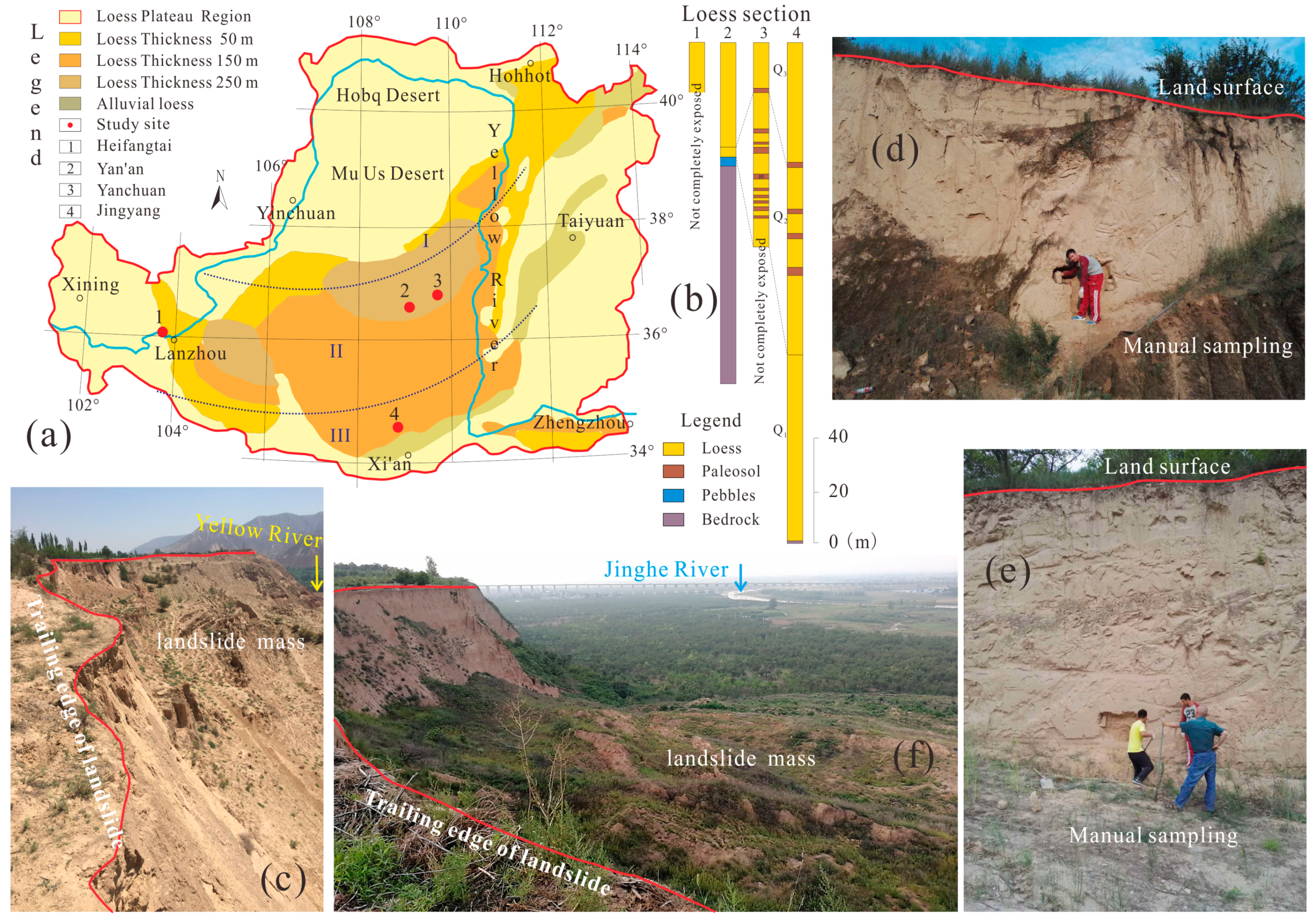
China’s loess covers an area of approximately 640,000 km2, accounting for approximately 4.9% of the world’s total loess. Distributed in the northern latitudes 33–37° and most developed in the Loess Plateau between 34–35°, the loess plateau area in China is approximately 440,000 km2 [26,48] (Figure 1a). The loess plateau is covered with thick quaternary sediments. Taking the perspective of engineering geology and soil mechanics, the grain size distribution of Chinese loess is between 0.01 mm and 0.05 mm. The content of silt exceeds 40% and is generally between 45–63%. Particles with a particle size larger than 0.25 mm (which belong to silt or silty clay) are almost completely missing, which is an important feature that distinguishes loess from other sediments. Liu’s study reported that the loess on the Chinese loess plateau showed gradually increasing grain size from northwest to southeast [49]. According to the change in loess facies, loess can be divided into three different facies belts: the (1) sandy loess zone (sand content > 5%), (2) loess zone (sand content < 5%), and (3) clayey loess zone (Figure 1a). This gradation is also an important factor in geological disasters such as liquefaction and refraction that involves water.
3.1.2. Analyzed Deposits and Properties
During this study, soil was taken from four different sites (Heifangtai, Yan’an New Area, Yanchuan, and Jingyang) of three loess zones (sandy loess, loess, and clayey loess) on the Loess Plateau (Figure 1c–f). The soil was taken from both landslide sections (Heifangtai and Jingyang) and excavation sections (Yan’an and Yanchuan). Only moist samples of upper Malan loess, which are related to human activities, were packed and transported to the laboratory for testing.
Site 1: The average annual rainfall of Heifangtai is 260 mm, the evaporation is over 1500 mm for many years, and the annual average temperature is 10 °C (Yongjing County People’s Government official website, http://www.gsyongjing.gov.cn). The Heifangtai sampling section consists of aeolian loess, alluvial silty clay, and gravel. The typical loess layer belongs to the late Pleistocene Malan loess, with a thickness of approximately 20–50 m. The thickness of the silty clay layer buried below the loess is approximately 4–17 m, and the thickness of the gravel layer below the silty clay layer is approximately 2–5 m. Neogene bedrock is under the gravel layer (Figure 1b,c).
Site 2: The average rainfall of Yan’an city over the years (1951–2012) was 531 mm, and the average annual temperature was 9.9 °C [50]. Yan’an New Area sampling section is located near the northern part of the Yan’an New Area. The excavation thickness of the project is 73 m, and loess-paleosol alternately appears in the section. A total of 10 layers of paleosol are exposed. This section contains 5–20 m of late Pleistocene Maland loess. The Lishi loess under the late Pleistocene Maland is several meters to more than 100 m thick. Only the middle and lower parts of the Lishi loess are revealed, while the upper part of the Lishi loess and the Wucheng loess are not exposed (Figure 1b,d).
Site 3: The average precipitation of Yanchuan country for many years (1984–2013) was 486.7 mm, and the average temperature for many years was 10.8 °C [51]. The thickness of the Malan loess in the Yanchuan section is approximately 45 m, and small pieces of calcareous concretion with scattering layers are occasionally found in this section. The thickness of the Lishi loess is approximately 60 m, but the thickness of the ancient soil layer is less than 60 m. There is unconformity contact between the upper part and the middle parts of the Lishi loess, indicating that there is obvious sedimentary discontinuity and denudation in the area. The Wucheng loess in the Yanchuan section is thicker than 80 m, and its underlying strata are Triassic sandstone (Figure 1b,e).
Site 4: The average annual precipitation in Yingyang country (1955–2012) was 460.7 mm, and the average annual temperature was 13.3 °C [52]. The profile of the Jingyang landslide is on the south bank of the Jinghe River, which is a typical loess tableland landform. This profile consists of late Pleistocene and Pleistocene loess-paleosol sequences. The upper part comprises typical Late Pleistocene eolian Malan loess with a thickness of approximately 10–15 m, and the lower part comprises middle Pleistocene Lishi loess with a thickness of approximately 40–54 m. Found at the foot of the slope, the ninth layer of loess in the late Pleistocene and the ninth layer of paleosol are exposed. The clay content of the Malan loess is approximately 20–30%, and the silt content exceeds 70%. Malan loess is a type of clay loess with fine grain sizes and a high clay content (Figure 1b,f).
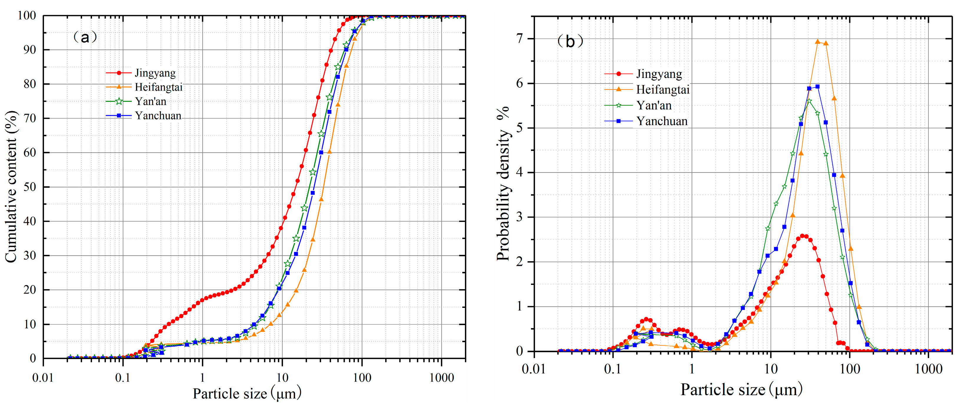
Laboratory tests were carried out on the remolded loess in the above four locations. The natural water content w0 (%), natural density ρ0 (g/cm3), dry density ρd (g/cm3), specific gravity (Gs), void ratio e, liquid limit LL (%), plastic limit PL (%), and plastic index Ip of these soils were measured in the laboratory (Table 1). The liquid–plastic limit was measured by the GYS-2 digital soil liquid–plastic limit tester (Nanjing Soil Instrument Factory Co. LTD, Nanjing, Jiangsu province, China, http://www.njtryq.cn/en/). Particle size analysis was conducted via a Bettersize2000 laser particle size distribution analyzer (Bettersize Instruments Ltd., Dandong, Liaoning province, China, https://www.bettersize.com.hk/) (Figure 2a,b).
3.2. Experiments
3.2.1. Permeability Measurements
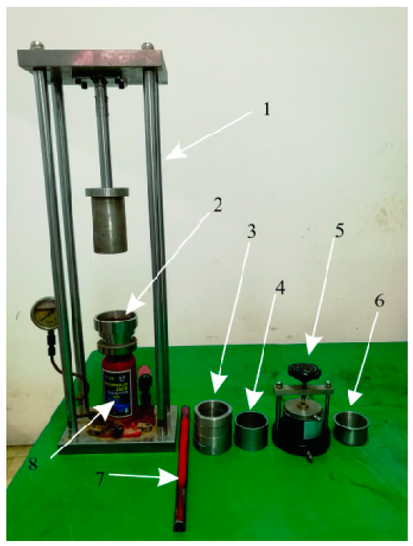
Loess samples from the four sites were brought to the laboratory. Samples were oven-dried at 105 °C, crushed, and passed through 2 mm meshes to remove impurities such as sand, calcium nodules, and plant roots, to test the soil clay. The remolded soil samples with different dry densities and water contents were mixed and configured with dry soil samples and cold water of known qualities by an electronic scale (Table 2) and were sealed and stored in a moisturizing dish for 24 h to ensure the even distribution of water. Each cylindrical sample of 61.8 × 40 mm was pressed individually with a hydraulic jack (5t) and stabilized for 15 min to ensure the sample had a stable structure (Figure 3).
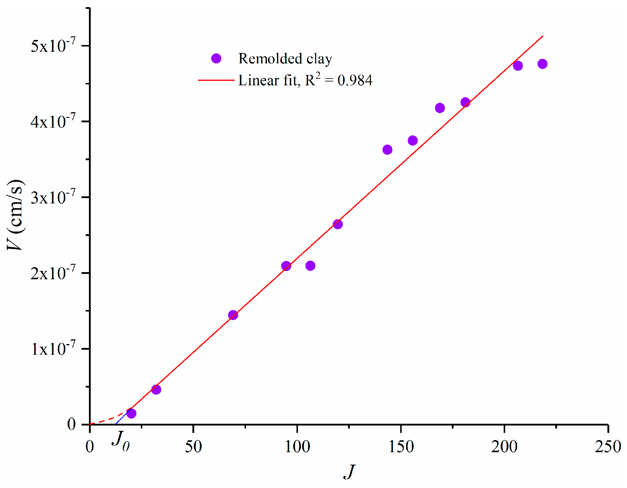
A prerequisite for the measurement of the saturation permeability coefficient is laminar fluid flow. Regarding cohesive soil, due to the large SSA of the soil particles, the surface interface between the particles and fluid is very strong, and it is easy to form strong and weak bonds between water and the surface of the soil particles. Furthermore, the pores of cohesive soil are relatively small. Therefore, in this soil, there is a minimum hydraulic gradient, also known as the initial hydraulic gradient, J0, and if the actual hydraulic gradient is less than J0, fluid does not flow. Prior to starting the test, we had to determine a suitable head difference in remolding the loess with the following criteria: (1) the head difference should be not too large. When the head difference is too large, the measured Ks value will be overestimated. Additionally, a large head difference will prolong the test period. Many studies have shown that, as the percolation time increases, the slow decomposition and migration of agglomerates in the clay leads to blockage of the percolation channels and, thus, reduces permeability [30] or, with the fluid discharge, increases seepage, which may not satisfy the Darcy flow assumptions and, thus, lead to the overestimation of the permeability coefficient [20]. (2) The head difference should be not too small. A small head difference may cause a large corresponding reading error. Additionally, if the head difference is too small, seepage may not start. According to Gu et al. [53], the results of remodeling clay permeability show that the initial hydraulic gradient may be J0 ≥ Δh/L = 12.5 (Figure 4), i.e., Δh ≥ 5 cm (for a TST-55 permeameter, the height of a sample is L = 4 cm). To shorten the observation time and ensure experimental accuracy, we selected a head test with a head difference of 5 cm for a 4-cm-high sample.
The Ks was measured by the variable head penetration test. The permeameter was a TST-55-type permeation instrument produced by Nanjing Soil Instrument Factory Co. Ltd., Nanjing, Jiangsu province, China, http://www.njtryq.cn/en (Figure 3). Prior to the sample being loaded, a thin layer of Vaseline was applied to the wall of the infiltration instrument to prevent sidewall leakage [20]. Afterwards, the sample was installed in place. The test started after back pressure + vacuum saturation, and the test was repeated 6–8 times. The calculation of Ks used the variable water head method in accordance with Darcy’s law:
where Ks represents the permeability coefficient at T (°C) (cm/s); 2.31 is the transformation factor of ln and log10; a represents the cross-sectional area of the variable head pipe (cm2); h1 and h2 represent the starting and ending heads (cm), respectively; and t is the time (s) for the head from h1 to h2. Regarding standardization, the Ks of the experimentally measured water temperature T (°C) was converted to a permeability coefficient at 20 °C:
where K20 represents the permeability coefficient (cm/s) of the sample at the standard temperature of 20 °C; μ20 represents the dynamic viscosity coefficient (kPa·s) of water at 20 °C; μT represents the dynamic viscosity of water at T (°C) (kPa·s).
3.2.2. Determination of BET-N2 Specific Surface Area
The SSA was determined by a large multistation automatic surface area and porosity analyzer (ASAP 2460) from Micromeritics Instrument (Shanghai) Ltd., Shanghai, China (http://mic.cnpowder.com.cn). The analysis bath temperature was −195.8 °C, and the adsorption medium was N2. The system automatically gave the SSA results.
4. Results and Analysis
The results of 139 laboratory tests (Table 3) were used to evaluate the ability of the KC equation to predict the permeability coefficient of remolded loess. This information, i.e., liquid limit, void ratio, and permeability coefficient values, is usually given in selected literature. A comprehensive method for evaluating the permeability coefficient of remolded loess based on the KC equation of the effective void ratio, ee and the specific surface area, SSA is presented.
4.1. Estimates of the Effective Void Ratio for Loess
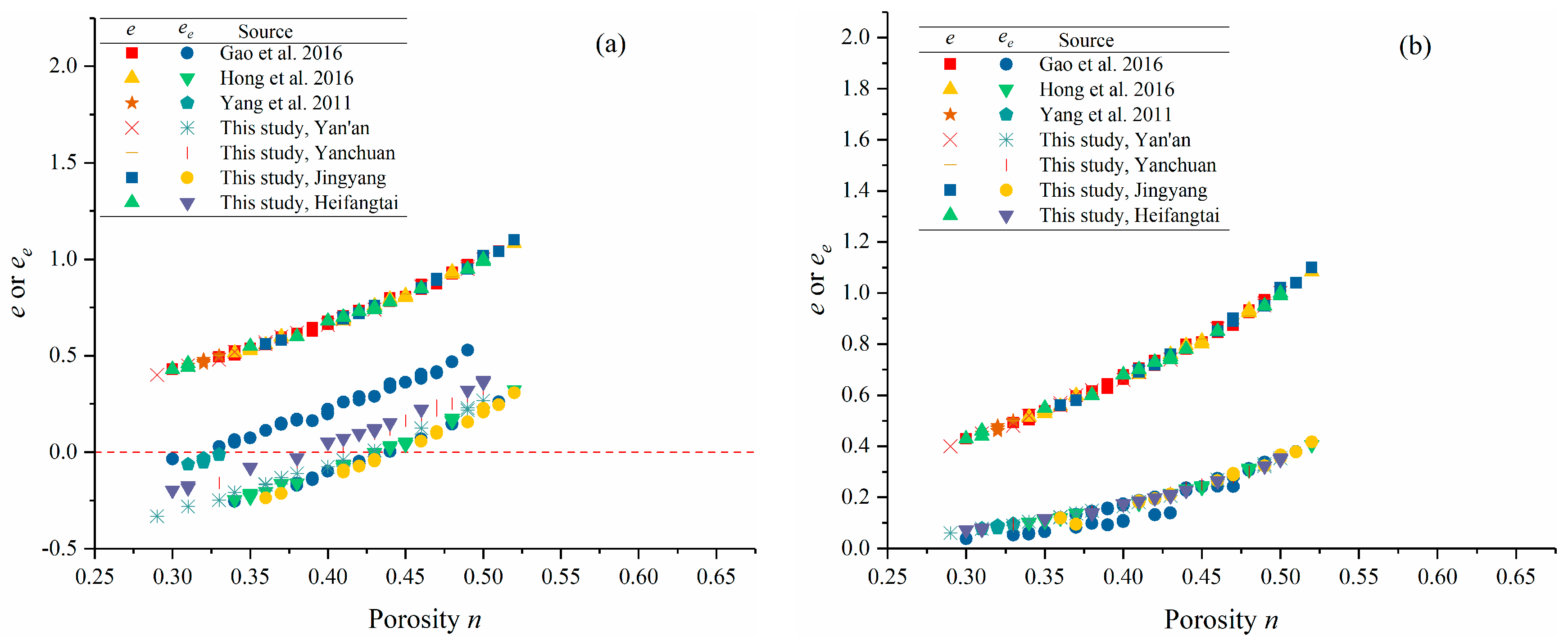
It is accepted that the ee is always smaller than the total void ratio, as shown in Figure 5. However, the ee estimated by Equation (8) in Figure 5 is negative, which is obviously not possible. The most basic conditions are as follows: the effective void ratio is ee > 0, the LL of loess is 22–52%, and the particle density of the soil is 2.65–2.75 g/cm3 (Malan loess). Suppose the LL of loess at a certain place is LL = 20%, ρs = 2.65 g/cm3. Take α0 = 0.9; according to the conditions of Equation (8) > 0, the total critical void ratio e > 0.477 is obtained. This critical value is obviously strongly dependent on the value of α0. However, differences in soil species, gradation, SSA and mineral composition values may result in different adsorbed bound moisture contents. Thus, according to Dang et al. [28], in the definition of α0, the parameter α0 cannot be obtained accurately, although α0 is approximately a constant for a given soil type.
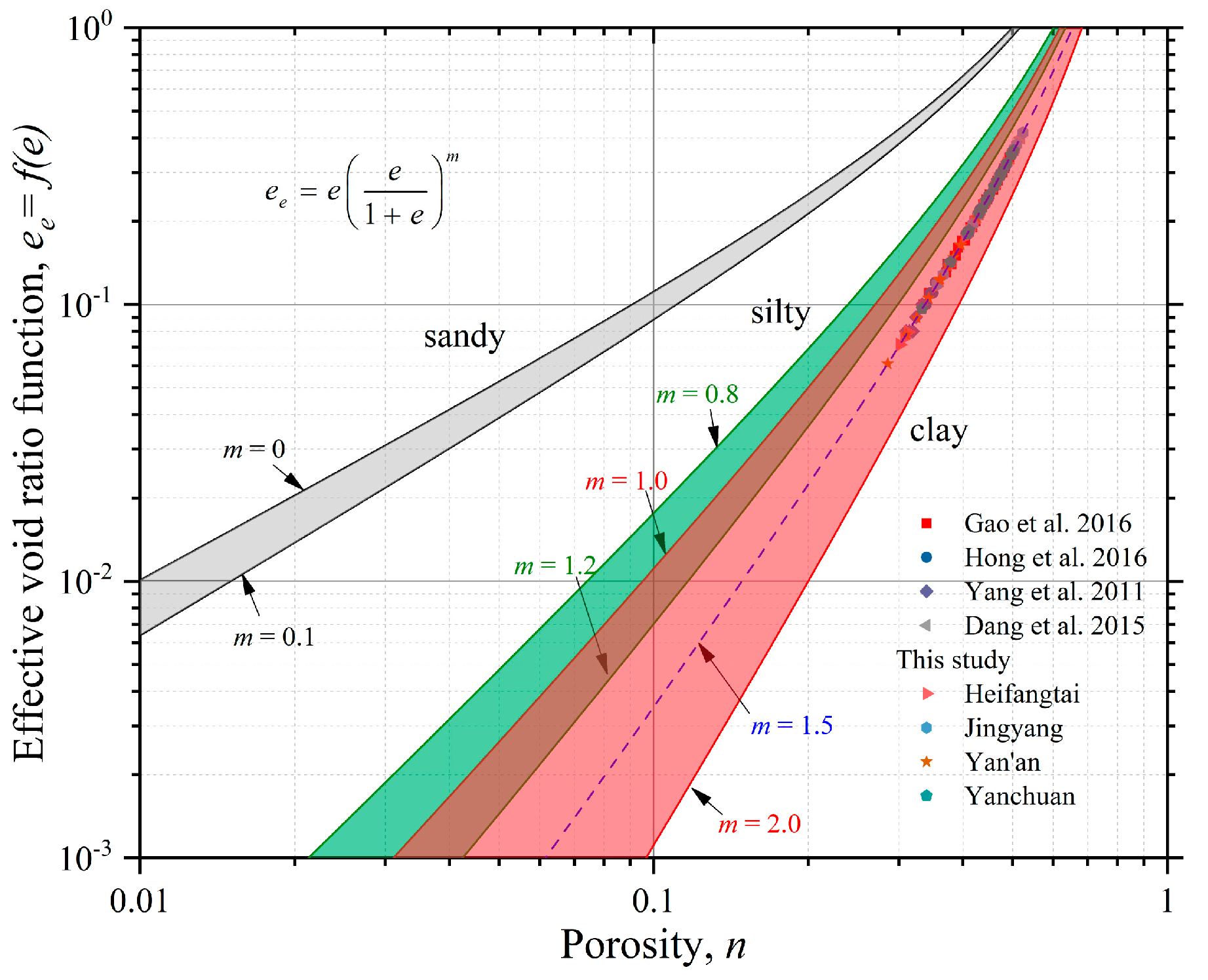
Considering that the effective void ratio must be a non-negative value, the result of Equation (14) is more satisfactory than that of Equation (8). Naturally, we needed evidence to prove the validity of Equation (14). We converted the ee of Equation (14) to a function of porosity, as shown in Figure 6. Values of m corresponded to sand, silt and clay, respectively. This coincided with research by Urumović and Urumović Sr [9] on the influences of the driving force factor and resistance factor on the porosity function. Obviously, the ee of different types of soil differs by orders of magnitude, and the smaller the porosity is, the more significant the difference will be (Figure 6). Figure 6 shows the loess results from various studies and the data from this study. The effective porosity ratio is very good, obeying Carman’s effective porosity function n3/(1 − n)2 [11].
4.2. Estimation of Specific Surface Area for Loess
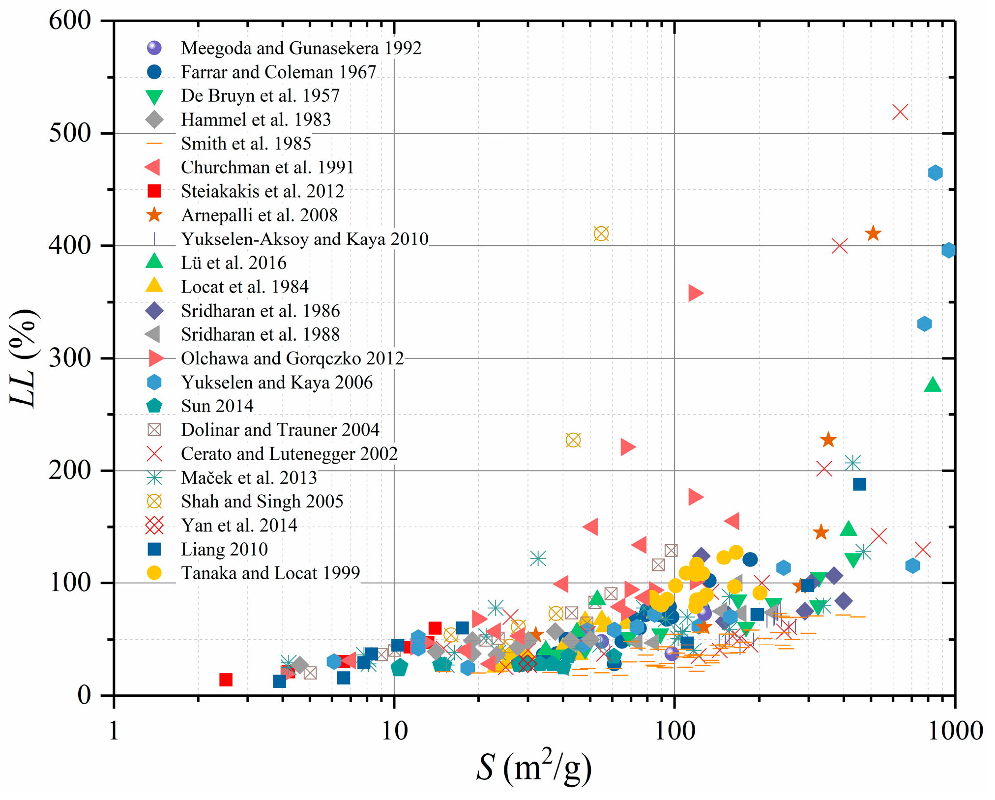
Extensive research has shown that the SSA of most clay soils can be evaluated by liquid limits. SSA and LL datum are usually given for test results for clay soil. We selected the SSA and the LL of clay soils from literature on different regions of the world, as shown in Figure 7 (total 311, LL < 600%). Figure 7 shows that there is a general trend between the SSA and LL—the SSA increases with increasing LL [46].
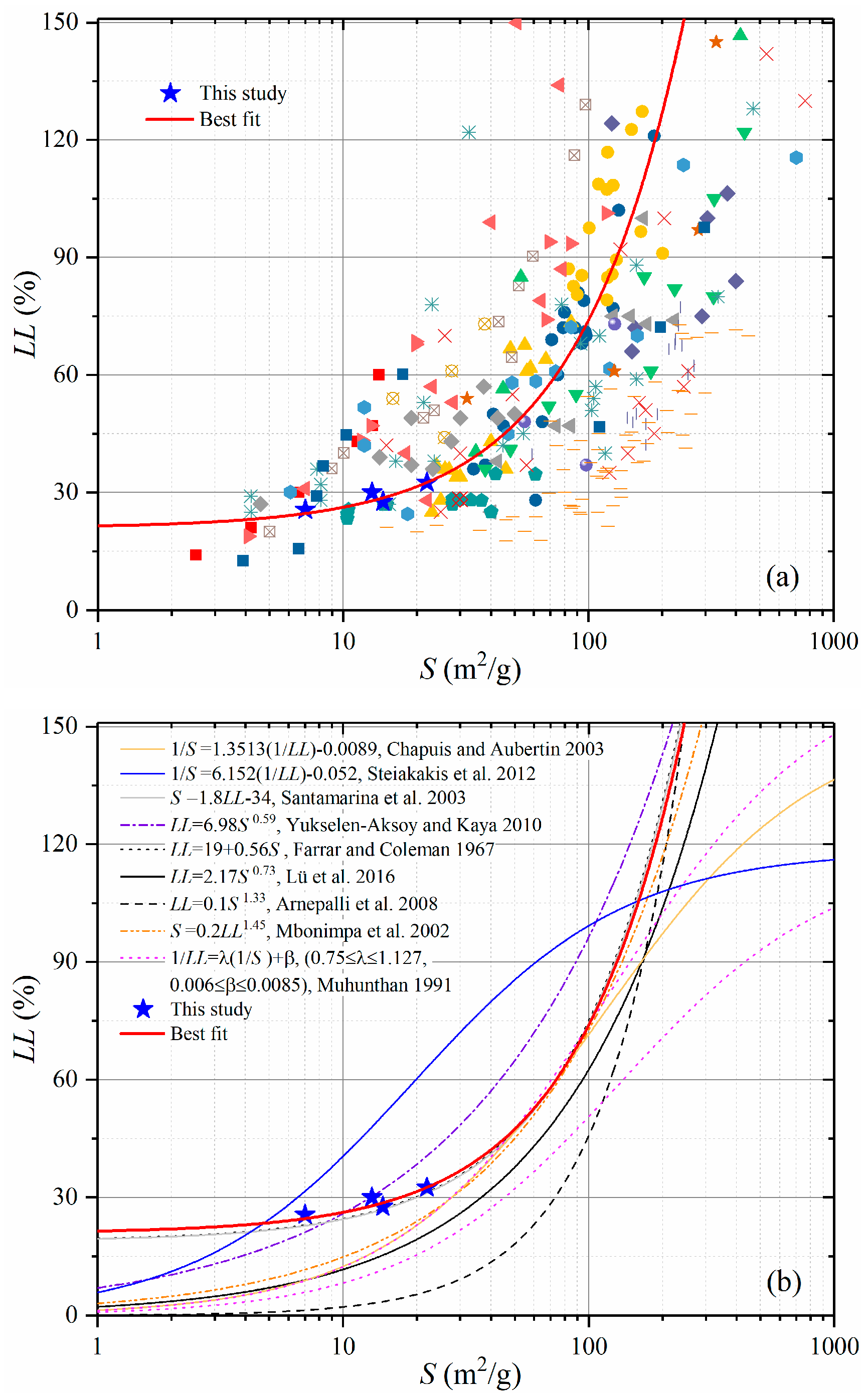
However, most (accounting for 95.2% of all data, or 296 data points) of the SSA data of clayey soil are LL < 150%. The LL of loess in China also is included in this range, so we analyzed data with an LL < 150%. Considering these data (LL < 150%), we obtained a relation between the LL and the SSA (Figure 8a).
This relation applies to LL < 150%, which underestimates the SSA value at the low LL or overestimates the SSA value at the high LL. However, when LL < 21.44%, this relation is invalid. Farrar and Coleman [24] and Santamarina et al. [23] report an LL less than a certain value (19% and 18.89%, respectively), so this prediction equation will not be used.
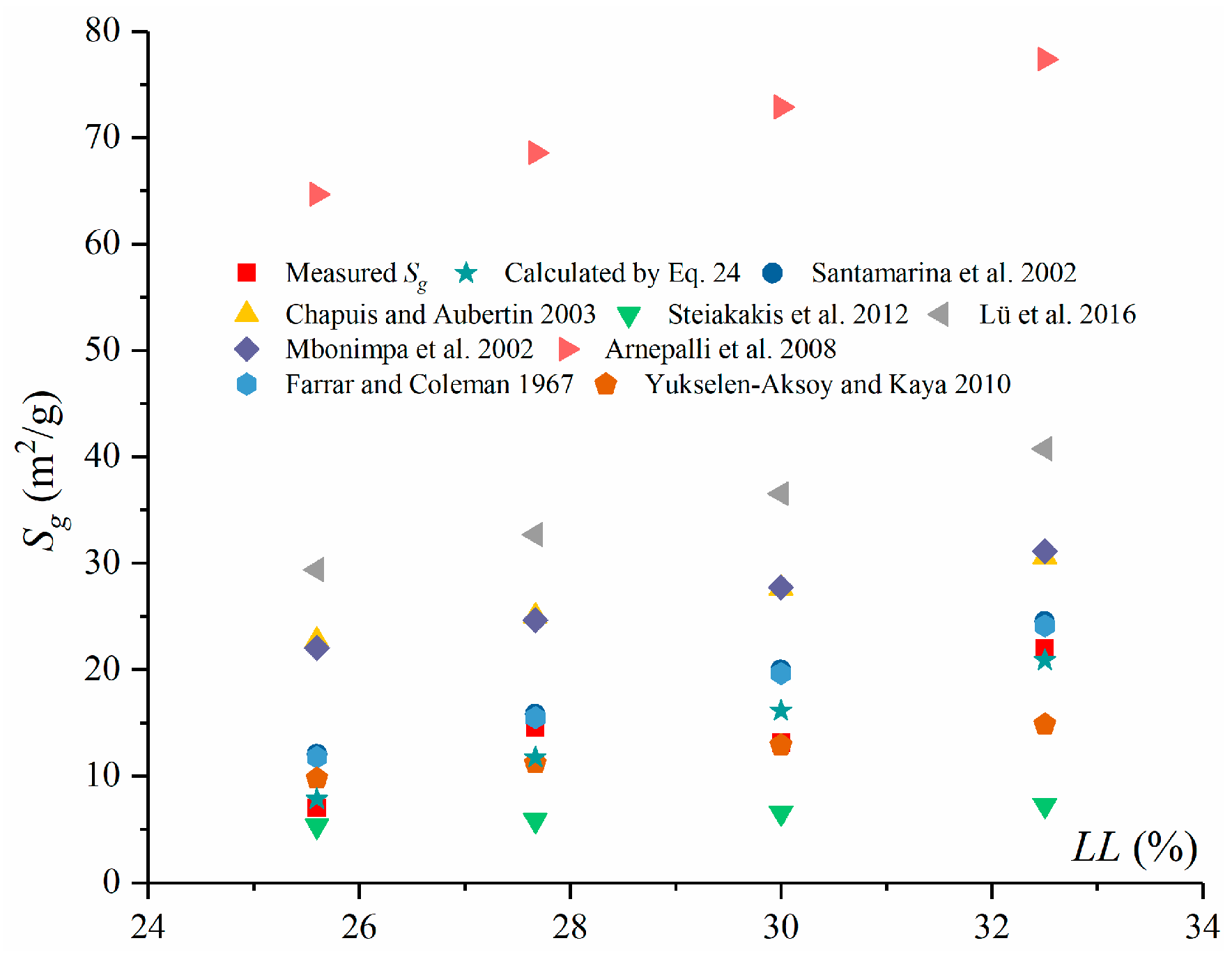
Figure 8b shows the correlation between the measured SSA of loess and the experience relationship proposed by many scholars, in the semilogarithmic coordinate system. As can be seen from Figure 8b, the SSA of loess is near the experience relationship of Farrar and Coleman [24], Santamarina et al. [23], Yukselen-Aksoy and Kaya [46]. Although the estimated relation curve of Yukselen–Aksoy and Kaya [46] is near the measured SSA value, this curve is for a given LL, below which the SSA will be overestimated and above which the SSA will be underestimated. Steiakakis et al. [43] underestimate the SSA value, and other empirical relationships overestimate the SSA value; the overestimation error can be approximately 10 times the actual value. According to Equation (1), the permeability is k ∝ (1/S2). If the SSA is estimated to be too low, the permeability will be overestimated; otherwise, the permeability will be underestimated.
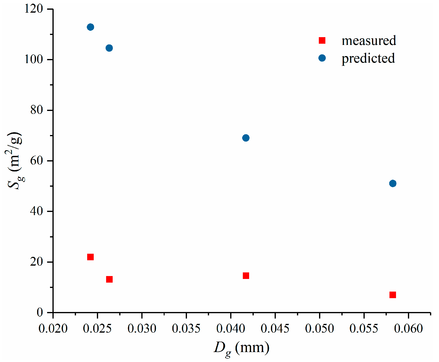
Figure 9 is a comparison between the estimated and measured values of the power function relation between the SSA and the geometric average particle size (Equation (16)). Figure 9 shows that the estimated SSA of Equation (16) is 3–8 times greater than the measured SSA. Thus, permeability is seriously underestimated because permeability is inversely proportional to the square of the SSA. Therefore, at least for remolded loess in the Loess Plateau of China, it is not appropriate to use Equation (16) to estimate the SSA.
Figure 10 shows the difference between the measured and predicted SSAs in more detail. The mean relative error (MRE) of the SSA predicted by Equation (23) is approximately 13.7% for loess. The MREs of Farrar and Coleman [24], Santamarina et al. [23] and Yukselen–Aksoy and Kaya [46] are 27.8% and 23.7%. Regarding Lü et al. [47] and Arnepalli et al. [45], the MREs of the predicted values for the SSA of loess are as high as 146% and 400%, respectively. The MREs of the other authors are greater than 50%.
4.3. Application and Evaluation
4.3.1. Verification of KC Equation Base on ne and Dg Correction
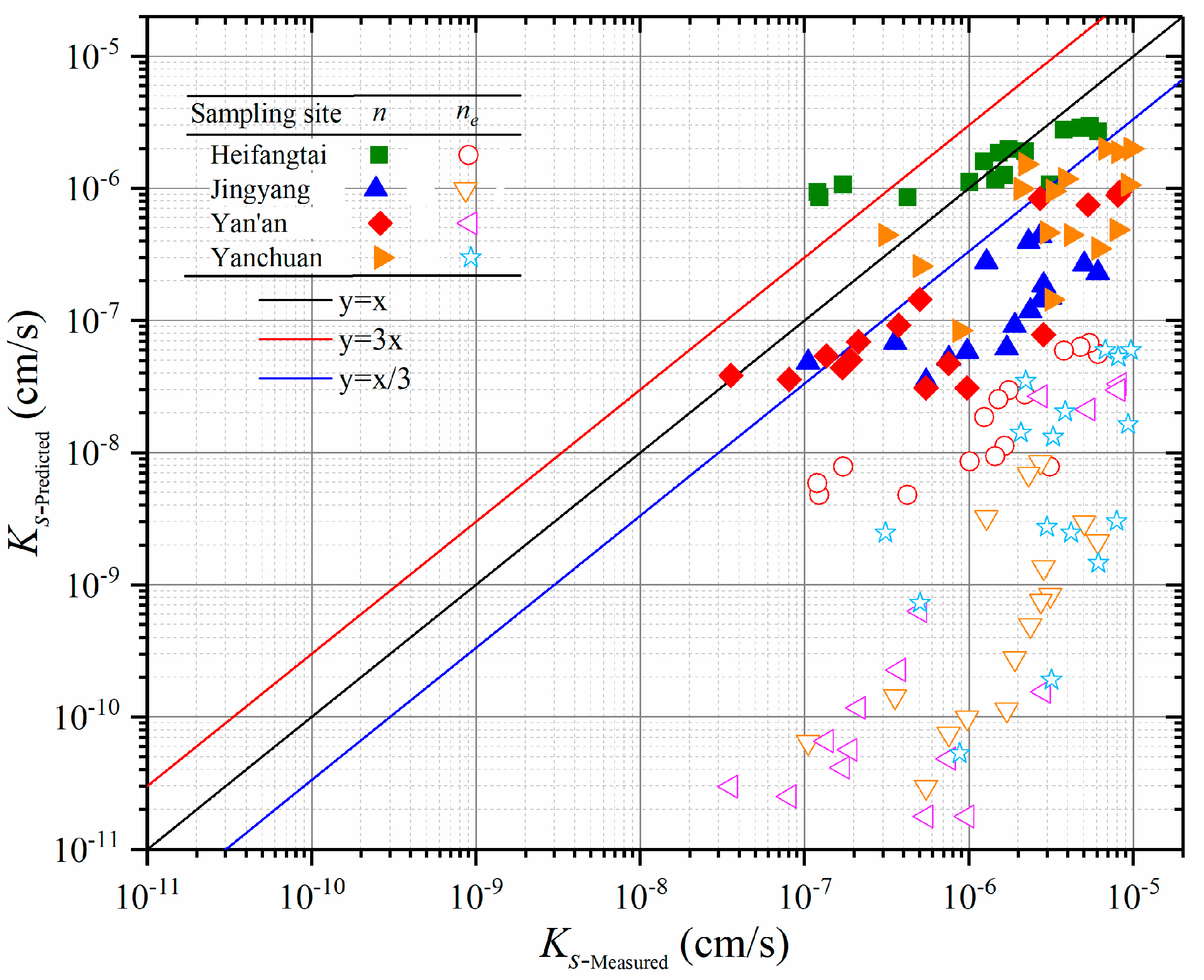
Looking at the description of the modified KC equation according to Urumović and Urumović Sr [8,9], the effects of the effective porosity and average reference particle size on the permeability of porous media are very important. The functional distribution of effective porosity for a reference particle size is graphically described as ne = f(Dg). However, the functional relationship is not clear. Therefore, the effective porosity for the conversion of the effective porosity ratio in this paper was used to calculate the permeability. Figure 11 shows the use of 64 results from this experiment to verify the modified KC equation based on the porosity geometric mean particle size Dg and the validity of the permeability coefficient prediction for remolded loess (Equation (6)). Figure 11 shows that the estimated KS value of Equation (6) highly underestimates the permeability coefficient of remolded loess, with a maximum deviation that can reach 104 orders of magnitude. Urumović and Urumović Sr [8,9] describe effective porosity as a function of the reference particle size; thus, the total porosity also depends on the reference particle size. Therefore, we used the effective porosity in the total porosity substitution of Equation (6) to estimate the permeability coefficient of the remolded loess, as shown in Figure 11. Although the reliability of the estimated KS value is greatly improved, some of the data are still far from the 1:1 line of the predicted and measured KS values, with a maximum deviation of almost 102 orders of magnitude. Although Equation (6) is applicable to the weak permeable layer of Croatian silty clay, the predicted KS value ranges between 1/3 and 3 times the measured KS value [8,9]. However, Equation (6) cannot be used to predict the permeability of remolded loess in China.
4.3.2. Verification of KC Equation Base on e and m Correction
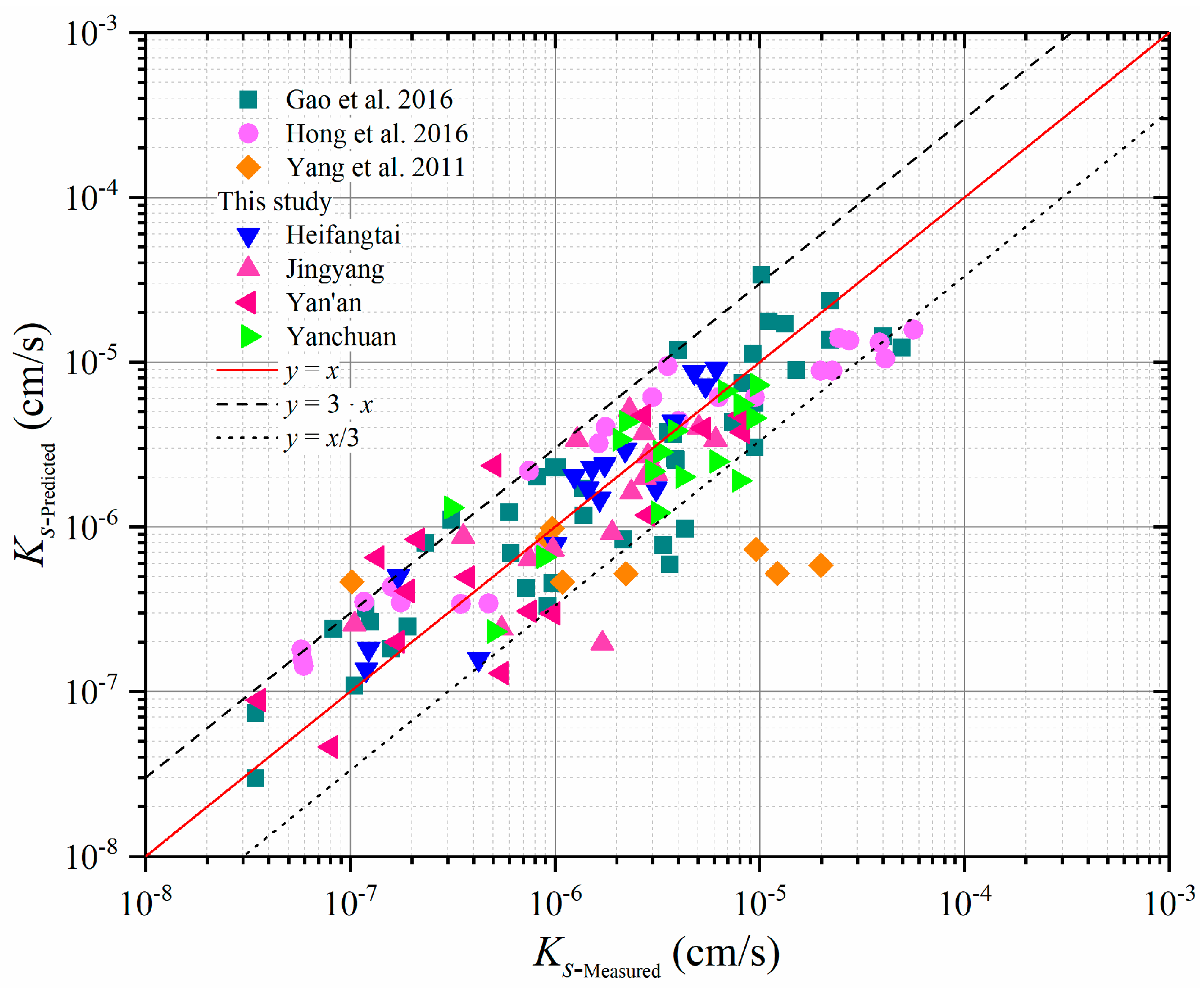
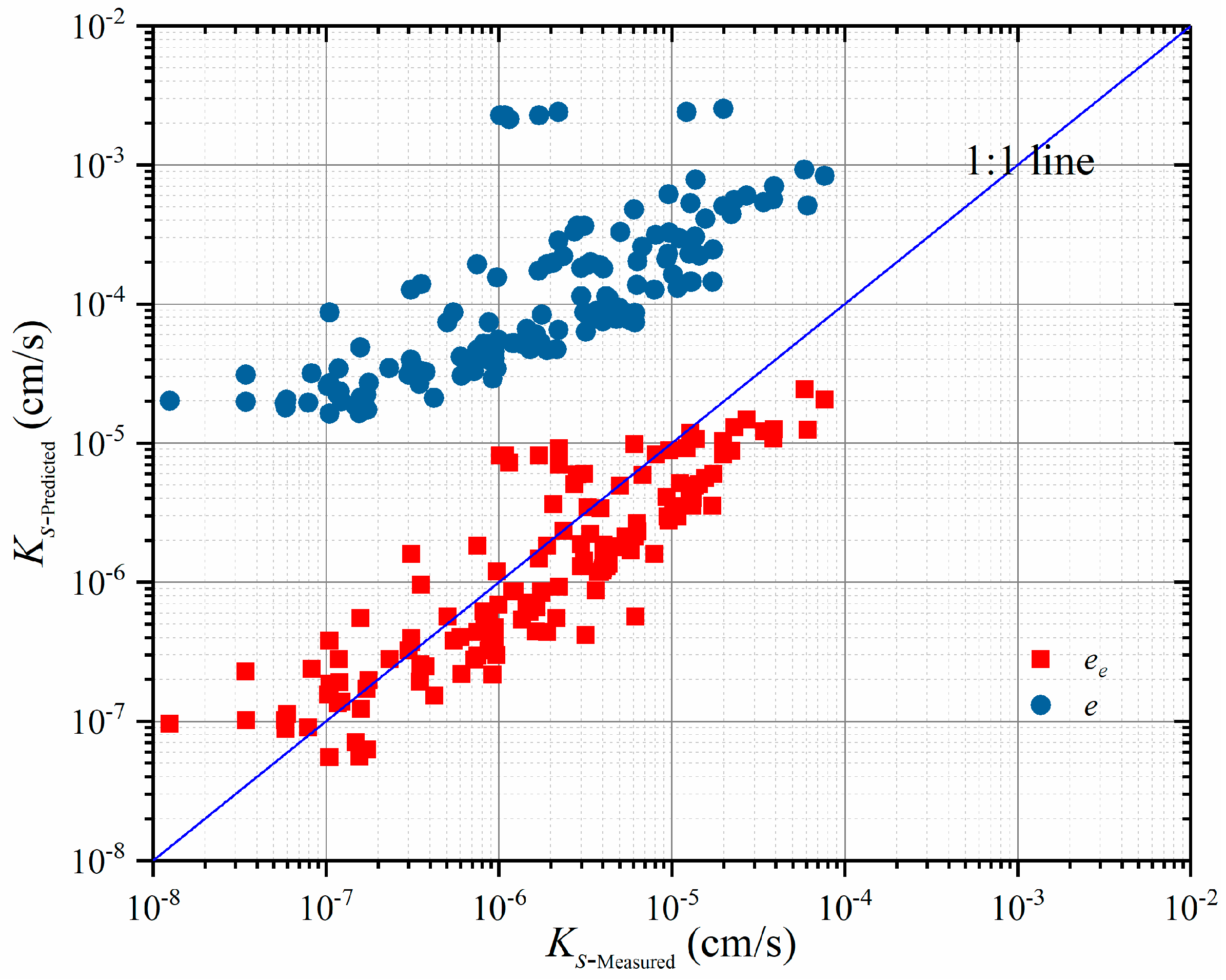
The results of the tests used here were derived from 42 results from remolded loess in the Yan’an New Area reported by Gao et al. [54], 25 results from remolded loess in the Yan’an New Area reported by Hong et al. [55], 8 results from a bentonite-loess mixed sample from Mongolia Xinghe County and loess samples from Yulin and 64 results from this experiment. The loess SSA values were estimated by Equation (23); these predicted and measured KS values are shown in Figure 12. To further test the reliability of the KS predictions of the KC equation based on the ee and SSA, the 64 measured KS values from four sites on the Loess Plateau were compared with the predicted KS values (Figure 11). Figure 12 shows that the predicted KS values were between 1/3 and 3 times the measured KS value and were within the expected range of laboratory penetration test results. An analysis of the existing loess literature and a comparison between the measured permeability coefficient and predicted permeability coefficient values indicate that most of the predicted KS values are between 1/3 and 3 times the measured KS values. This is within the expected range of laboratory penetration test results, which indicates that the modified KC equation based on the ee and the SSA is effective in predicting the hydraulic conductivity of remolded loess.
5. Discussion
Regarding remolded loess, if SSA and ee information of loess can be accurately obtained, and when adequate preventive measures are taken in the permeation test (for example, homogeneity control in the preparation of the remolded sample), the modified KC equation can be used to predict the Ks of saturated remolded loess. The precision of the penetration test depends on the process control and the homogeneity (or inherent variability) of the soil sample, and the prediction precision is mainly derived from the uncertainty of the ee and SSA prediction.
5.1. Uncertainty of the Effective Porosity Ratio
According to a large number of existing studies, the effective porosity of clay soil should be considered [18,27,31]. When the effective porosity is significantly lower than the total porosity, but the effective porosity is assumed to be equal to the total porosity, the percolation velocity will be overestimated (Figure 13).
Because effective pore data are difficult to measure, it is necessary to estimate effective pore data based on other data. Dang et al. [28] and Kou et al. [29] estimated the ee based on the LL and PL, respectively. Figure 5a shows that the Dang et al. [28] estimation relationship is limited and not applicable to clay with a small total porosity. Kou et al. [29] also have the same problem. Yang et al. [53], from the point of view of microstructures, express the ee as a percentage of the total visual field area with large and medium porosity. A crucial question here is how we can determine this representative vision. Three ee relationships were proposed by Li et al. [70]. These relationships may seem simple, but some variables are difficult to obtain (e.g., combination of water content), and the test processes are difficult to control.
Although many researchers have reported useful developments on the effective pore estimation method, the estimation of the ee is attributed with uncertainty related to (1) the introduction of experimental errors and (2) the definition of effective porosity (e.g., field water capacity, moving water volume, and immovable water volume).
5.2. Uncertainty in the Specific Surface Area
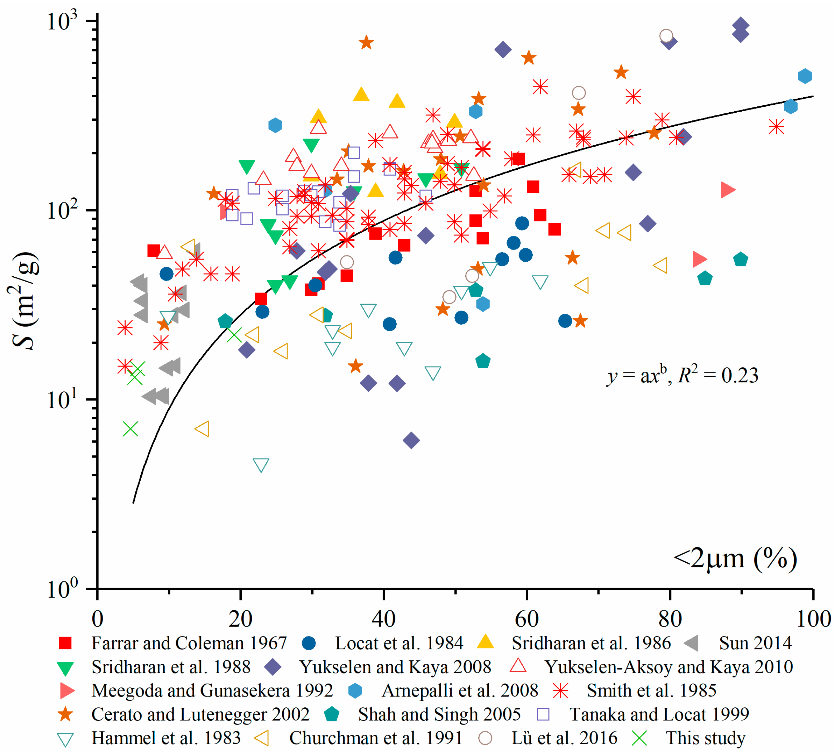
There are three main aspects of uncertainty in the estimation of SSA values. (1) The uncertainty is closely related to the test method. According to existing research, different test methods have different test results [45,71]. The EGME method is recommended by Arnepalli et al. [45] because this method is cost effective. Yukselen and Kaya [71] recommended the MB method because the MB method is simpler and more reliable than the EGME method in soil science and clay mineralogy, where the internal surface area is very important. The results of measurements with the N2 adsorption method only show the surface area of granular material, which seems to be most suitable for the application of the KC equation to a large number of loess samples with agglomerates, aggregates, coating and cementation. (2) Uncertainties also are related to clay content (<2 μm, (%)). Figure 14 shows that the SSA tend to increase with increasing clay content. (3) Finally, uncertainties can be related to the estimation relationship. Since most such estimates are derived from SSA measurements and other physical properties of the soil, estimation relationship error may be derived from the SSA test method. The SSA predicted by Chapuis and Aubertin [21], for example, for Champlain clay is S ± 25%.
5.3. Influence of the Uniformity of Remolded Specimens
Ensuring the homogeneity of a sample is one of the most important and basic conditions of sample preparation. The process of sample preparation is affected by various factors. Even with the same initial dry density and initial water content, prepared samples may demonstrate a great deal of randomness in various parameters.
- (1).
- The sample preparation method for remolded soil may affect the results of the osmotic test. Some studies show that the seepage stability of static compacted specimens is obviously superior to that of impact and kneading methods [72]. Concurrently, the stability of a static compacted specimen also is affected by the initial dry density and moisture content. Generally, the stability of compacted specimens increases with increasing initial dry density and water content. Regarding impacted samples, the lower part of the sample is usually denser than the upper layer, and local blockage of the sample occurs [21]. Accompanying the decrease in porosity, the seepage path zigzags more. Simultaneously, the site surface between the layers forms a relatively dense structure, similar to the weak permeable layer in the stratum, resulting in the underestimation of the measured Ks. Additionally, for a specimen with a low initial water content, the Ks of the specimen bottom may increase due to the occurrence of microcracks during compaction.
- (2).
- Remolded soil samples may be affected by the predominance of seepage in the formation of larger pores. Although different authors give different pore boundary diameters for large pores (or larger pores or macropores), it is difficult to measure and quantify this value under high seepage [73]. Jang et al. [74] showed that, according to simulation results of a pore network model, 10% of the large holes may contribute to 50% of the total flow. However, this is not the true reflection of the soil system.
- (3).
- Tortuous/pore-throat effect. Although the structures of joints, fissures and aggregates are destroyed in remolded soil, a more uniform pore structure is formed by the remolding process. However, compacted clay is composed of different mineral particles. Under the influence of compaction energy, macropores may be discontinuous and the action of pore throats will restrict the adjacent large pores [75]. The existence of the pore throats greatly increases the seepage paths. The results of a study by Kucza and Ilek [76] on the permeability of irregularly shaped specimens are described as follows. Kucza and Ilek [76] report that water conductivity measurement errors are minimal for these specimens due to the continuous variation in the sample cross section, and the lateral surface change of a sample is the dominant factor of measurement errors. That is, we can see an irregular sample as a single irregularly shaped capillary and the lateral surface can be seen as a meandering flow path, i.e., tortuosity. The seepage path becomes longer due to the limitation of the pore throat, that is, the lateral surface described by Kucza and Ilek [76] of the sample is increased, which results in the overestimation or underestimation of the measured Ks. However, Olsen [19] does not consider the tortuous path of the seepage to completely explain the difference between the predicted and the measured Ks.
5.4. Test Process Control
According to the current geotechnical test standards, the true accuracy of the penetration test method is unknown, so we cannot estimate the error range [21]. Consequently, we need to strictly control the penetration test process to obtain data that can reflect the permeability of the material as truthfully as possible. First, for the seepage samples tested in the rigid wall permeability meter, sidewall leakage will cause the measurement error to be several orders of magnitude greater. Therefore, measurements must be taken to prevent lateral wall leakage. Second, to improve the saturation degree of the sample as much as possible, the steady seepage condition must be reached [77]. A low saturation will inevitably cause the inclusion of trapped bubbles in the fluid and two-phase flow. Finally, for a clay soil, a suitable head difference is an important condition to ensure a steady flow. Accompanying low saturation and a large water head difference, there will be a slip effect (Forchheimer effect) at the interface between the flow channel and the fluid. Concurrently, the migration of fine particles and the expansion of the channel will be aggravated without satisfying laminar flow conditions.
6. Conclusions
Here, estimation algorithms of the SSA and ee of clay with the KC equation are reviewed. By fitting a large number of clay soil LL and SSA data, a good linear relationship in semilogarithmic coordinates was achieved for the LL and SSA. Using a large number of remodeling experimental data of loess permeability, a modification to the KC equation based on the SSA and ee estimation algorithm enabled the permeability coefficient of remolded loess to be predicted. The predicted Ks ranged between 1/3 and three times the laboratory test value. The difference between the predicted and measured Ks was likely caused by the uniformity of remolded specimens, unreliable test process control, inaccurate estimation of the ee and inaccurate estimates of SSA. The effect of the ee on the prediction of the clay permeability coefficient cannot be ignored, and the permeability coefficient can be overestimated by 2–3 orders of magnitude. Although the error is associated with the Ks prediction method, the method can quickly estimate the permeability coefficient of a series of remolded loess samples, as long as the total pore ratio and SSA values have been determined.
Author Contributions
B.H. and X.L. conceived and designed the research ideas, supervised the research; B.H. conducted data analysis and prepared the manuscript; Q.X. and J.M. mainly carried out the data collection; L.W. and L.L. conducted the review of it, made English corrections, and contributed to manuscript preparation. All authors have read and agreed to the published version of the manuscript.
Funding
This research was funded by the Natural Science Foundation of China, grant numbers 41572264 and 41877225 and the Fundamental Research Funds for the Central Universities, CHD, grant number 300102268717.
Conflicts of Interest
The authors declare no conflict of interest.
References
- Meegoda, N.; Gunasekera, S. A New Method to Measure the Effective Porosity of Clays. Geotech. Test. J. 1992, 15, 340–351. [Google Scholar] [CrossRef]
- Boadu, F.K. Hydraulic Conductivity of Soils from Grain-Size Distribution: New Models. J. Geotech. Geoenviron. Eng. 2000, 126, 739–746. [Google Scholar] [CrossRef]
- Ahuja, L.R.; Naney, J.W.; Green, R.E.; Nielsen, D.R. Macroporosity to Characterize Spatial Variability of Hydraulic Conductivity and Effects of Land Management. Soil Sci. Soc. Am. J. 1984, 48, 699–702. [Google Scholar] [CrossRef]
- Ahuja, L.R.; Naney, J.W.; Williams, R.D. Estimating Soil Water Characteristics from Simpler Properties or Limited Data. Soil Sci. Soc. Am. J. 1985, 49, 1100–1105. [Google Scholar] [CrossRef]
- Schaap, M.G.; Lebron, I. Using microscope observations of thin sections to estimate soil permeability with the Kozeny–Carman equation. J. Hydrol. 2001, 251, 186–201. [Google Scholar] [CrossRef]
- Regalado, C.M.; Muñoz-Carpena, R. Estimating the saturated hydraulic conductivity in a spatially variable soil with different permeameters: A stochastic Kozeny–Carman relation. Soil Tillage Res. 2004, 77, 189–202. [Google Scholar] [CrossRef]
- Song, J.; Chen, X.; Cheng, C.; Wang, D.; Lackey, S.; Xu, Z. Feasibility of grain-size analysis methods for determination of vertical hydraulic conductivity of streambeds. J. Hydrol. 2009, 375, 428–437. [Google Scholar] [CrossRef]
- Urumović, K.; Urumović, K., Sr. The effective porosity and grain size relations in permeability functions. Hydrol. Earth Syst. Sci. Discuss. 2014, 11, 6675–6714. [Google Scholar] [CrossRef]
- Urumović, K.; Urumović Sr, K. The referential grain size and effective porosity in the Kozeny–Carman model. Hydrol. Earth Syst. Sci. 2016, 20, 1669–1680. [Google Scholar] [CrossRef] [Green Version]
- Kozeny, J. Uber Kapillare Leitung der Wasser in Boden. R. Acad. Sci. Vienna Proc. Cl. I 1927, 136, 271–306. [Google Scholar]
- Carman, P.C. Permeability of saturated sands, soils and clays. J. Agric. Sci. 1939, 29, 262–273. [Google Scholar] [CrossRef]
- Carman, P.C. Flow of Gas Through Porous Media; Butterworths Scientific Publications: London, UK, 1956. [Google Scholar]
- Bear, J. Dyinamics of Fluid in Porous Media; Elsevier: New York, NY, USA, 1972. [Google Scholar]
- Todd, D.K. Ground Water Hydrology; John Wiley and Sons, Inc.: New York, UY, USA, 1959. [Google Scholar]
- Irani, R.; Callis, C. Particle Size: Measurement, Interpretation and Application; John Wiley and Sons: New York, NY, USA, 1963. [Google Scholar]
- Taylor, D.W. Fundamentals of Soil Mechanics; Wiley: New York, NY, USA, 1948; p. xii. [Google Scholar]
- Michaels, A.S.; Lin, C.S. Permeability of kaolinite. Ind. Eng. Chem. 1954, 46, 1239–1246. [Google Scholar] [CrossRef]
- Carrier, W.D., III. Goodbye, Hazen; Hello, Kozeny-Carman. J. Geotech. Geoenviron. Eng. 2003, 129, 1054–1056. [Google Scholar] [CrossRef]
- Olsen, H.W. Hydraulic flow through saturated clays. In Clays Clay Miner; Ingerson, E., Ed.; Springer: Pergamon, Turkey, 1962; pp. 131–161. [Google Scholar] [CrossRef]
- Zhang, M.; Zhu, X.; Yu, G.; Yan, J.; Wang, X.; Chen, M.; Wang, W. Permeability of muddy clay and settlement simulation. Ocean Eng. 2015, 104, 521–529. [Google Scholar] [CrossRef]
- Chapuis, R.P.; Aubertin, M. On the use of the Kozeny–Carman equation to predict the hydraulic conductivity of soils. Can. Geotech. J. 2003, 40, 616–628. [Google Scholar] [CrossRef]
- Ren, X.; Zhao, Y.; Deng, Q.; Kang, J.; Li, D.; Wang, D. A relation of hydraulic conductivity-void ratio for soils based on Kozeny-Carman equation. Eng. Geol. 2016, 213, 89–97. [Google Scholar] [CrossRef]
- Santamarina, J.C.; Klein, K.A.; Wang, Y.H.; Prencke, E. Specific surface: Determination and relevance. Can. Geotech. J. 2002, 39, 233–241. [Google Scholar] [CrossRef]
- Farrar, D.M.; Coleman, J.D. The correlation of surface area with other properties of nineteen British clay soils. J. Soil Sci. 1967, 18, 118–124. [Google Scholar] [CrossRef]
- Li, X.-A.; Li, L.-C. Quantification of the pore structures of Malan loess and the effects on loess permeability and environmental significance, Shaanxi Province, China: An experimental study. Environ. Earth Sci. 2017, 76, 523. [Google Scholar] [CrossRef]
- Li, X.-A.; Li, L.-C.; Song, Y.-X.; Hong, B.; Wang, L.; Sun, J.-Q. Characterization of the mechanisms underlying loess collapsibility for land-creation project in Shaanxi Province, China—A study from a micro perspective. Eng. Geol. 2018, 249, 77–88. [Google Scholar] [CrossRef]
- Koponen, A.; Kataja, M.; Timonen, J. Permeability and effective porosity of porous media. Phys. Rev. E 1997, 56, 3319–3325. [Google Scholar] [CrossRef]
- Dang, F.N.; Liu, H.W.; Wang, X.W.; Xue, H.B.; Ma, Z.Y. Researching clayey empirical formula of permeability coefficient based on the theory of effective porosity ratio. Chin. J. Rock Mech. Eng. 2015, 34, 1909–1917. [Google Scholar]
- Kou, L.; Xu, J.G.; Wang, B. Research on Grouting Infiltration Mechanism for Time-Dependent Viscous Slurry Considering Effective Void Ratios in Saturated Clay. Appl. Math. Mech. 2018, 39, 83–91. [Google Scholar]
- Bodman, G.B.; Harradine, E.F. Mean Effective Pore Size and Clay Migration during Water Percolation in Soils. Soil Sci. Soc. Am. J. 1939, 3, 44–51. [Google Scholar] [CrossRef]
- Stephens, D.B.; Hsu, K.-C.; Prieksat, M.A.; Ankeny, M.D.; Blandford, N.; Roth, T.L.; Kelsey, J.A.; Whitworth, J.R. A comparison of estimated and calculated effective porosity. Hydrogeol. J. 1998, 6, 156–165. [Google Scholar] [CrossRef]
- Muhunthan, B. Liquid limit and surface area of clays. Géotechnique 1991, 41, 135–138. [Google Scholar] [CrossRef]
- Salem, H.S. Application of the Kozeny-Carman Equation to Permeability Determination for a Glacial Outwash Aquifer, Using Grain-size Analysis. Energy Sources 2001, 23, 461–473. [Google Scholar] [CrossRef]
- Korvin, G. Permeability from Microscopy: Review of a Dream. Arabian J. Sci. Eng. 2016, 41, 2045–2065. [Google Scholar] [CrossRef]
- Sepaskhah, A.R.; Tabarzad, A.; Fooladmand, H.R. Physical and empirical models for estimation of specific surface area of soils. Arch. Agron. Soil Sci. 2010, 56, 325–335. [Google Scholar] [CrossRef]
- Shirazi, M.A.; Boersma, L. A Unifying Quantitative Analysis of Soil Texture. Soil Sci. Soc. Am. J. 1984, 48, 142–147. [Google Scholar] [CrossRef]
- De Bruyn, C.M.A.; Collins, L.F.; Williams, A.A.B. The Specific Surface, Water Affinity, and Potential Expansiveness of Clays. Clay Miner. Bull. 1957, 3, 120–128. [Google Scholar] [CrossRef]
- Hammel, J.E.; Sumner, M.E.; Burema, J. Atterberg Limits as Indices of External Surface Areas of Soils1. Soil Sci. Soc. Am. J. 1983, 47, 1054–1056. [Google Scholar] [CrossRef]
- Smith, C.W.; Hadas, A.; Dan, J.; Koyumdjisky, H. Shrinkage and Atterberg limits in relation to other properties of principal soil types in Israel. Geoderma 1985, 35, 47–65. [Google Scholar] [CrossRef]
- Wetzel, A. Interrelationships between porosity and other geotechnical properties of slowly deposited, fine-grained marine surface sediments. Mar. Geol. 1990, 92, 105–113. [Google Scholar] [CrossRef]
- Churchman, G.J.; Burke, C.M.; Parfitt, R.L. Comparison of various methods for the determination of specific surfaces of sub soils. J. Soil Sci. 1991, 42, 449–461. [Google Scholar] [CrossRef]
- Churchman, G.J.; Burke, C.M. Properties of sub soils in relation to various measures of surface area and water content. J. Soil Sci. 1991, 42, 463–478. [Google Scholar] [CrossRef]
- Steiakakis, E.; Gamvroudis, C.; Alevizos, G. Kozeny-Carman Equation and Hydraulic Conductivity of Compacted Clayey Soils. Geomaterials 2012, 2, 37–41. [Google Scholar] [CrossRef] [Green Version]
- Mbonimpa, M.; Aubertin, M.; Chapuis, R.P.; Bussière, B. Practical pedotransfer functions for estimating the saturated hydraulic conductivity. Geotech. Geol. Eng. 2002, 20, 235–259. [Google Scholar] [CrossRef]
- Arnepalli, D.N.; Shanthakumar, S.; Hanumantha Rao, B.; Singh, D.N. Comparison of Methods for Determining Specific-surface Area of Fine-grained Soils. Geotech. Geol. Eng. 2008, 26, 121–132. [Google Scholar] [CrossRef]
- Yukselen-Aksoy, Y.; Kaya, A. Method dependency of relationships between specific surface area and soil physicochemical properties. Appl. Clay Sci. 2010, 50, 182–190. [Google Scholar] [CrossRef]
- Lȕ, H.B.; Qian, L.Y.; Chang, H.S.; Liu, L.; Zhao, Y.L. Comparison of several methods for determining specific surface area of clayey soils. Chin. J. Geotech. Eng. 2016, 38, 124–131. [Google Scholar]
- Liu, T.; Ding, Z. Chinese loess and the paleomonsoon. Annu. Rev. Earth Planet. Sci. 1998, 26, 111–145. [Google Scholar] [CrossRef]
- Liu, T.S. The Loess Deposits in China; Science Press: Beijing, China, 1965. [Google Scholar]
- Li, B.; Wang, L. Statistical analysis of precipitation in the past 60 years in Yan’an. Shaanxi Water Res. 2015, 126–129. [Google Scholar] [CrossRef]
- Dang, X.; Liu, H. Analysis of climate change trend of Yanchuan County of Shaanxi Province in recent 30 years. Beijing Agric. 2015, 143–144. [Google Scholar] [CrossRef]
- Shang, X.; Zhao, X.; Gao, F.; Zhang, Y.; Ma, L. Analysis of climate change characteristics of Jingyang in the last 58 years. J. Shaanxi Meteorol. 2014, 1–4. [Google Scholar] [CrossRef]
- Gu, Z.W.; Sun, B.N.; Dong, Y.N. Testing Study of Permeability of the Original Clay, Recomposed Clay and Improved Clay with Stabilizer ZDYT-1. Chin. J. Rock Mech. Eng. 2003, 22, 505–508. [Google Scholar]
- Gao, Y.Y.; Qian, H.; Yang, J.; Feng, J.; Huo, C.C. Indoor experimental study on permeability characteristics of remolded Malan Loess. South-to-North Water Transf. Water Sci. Technol. 2016, 14, 130–136. [Google Scholar]
- Hong, B.; Li, X.A.; Chen, G.D.; Luo, J.W.; Li, L.C. Experimental study of permeability of remolded Malan Loess. J. Eng. Geol. 2016, 24, 276–283. [Google Scholar]
- Yang, B.; Zhang, H.Y.; Zhao, T.Y.; Liu, J.S.; Chen, H. Responsibility of permeability of modified loess soil on microstructure. Hydrogeol. Eng. Geol. 2011, 38, 96–101. [Google Scholar]
- Locat, J.; Lefebvre, G.; Ballivy, G. Mineralogy, chemistry, and physical properties interrelationships of some sensitive clays from Eastern Canada. Can. Geotech. J. 1984, 21, 530–540. [Google Scholar] [CrossRef]
- Sridharan, A.; Rao, S.M.; Murthy, N.S. Liquid Limit of Montmorillonite Soils. Geotech. Test. J. 1986, 9, 156–159. [Google Scholar] [CrossRef]
- Sridharan, A.; Rao, S.M.; Murthy, N.S. Liquid limit of kaolinitic soils. Géotechnique 1988, 38, 191–198. [Google Scholar] [CrossRef]
- Olchawa, A.; Gorączko, A. The relationship between the liquid limit of clayey soils, external specific surface area and the composition of exchangeable cations/Zależność granicy płynności od zewnętrznej powierzchni właściwej i składu kationów w naturalnym kompleksie wymiennym. J. Water Land Dev. 2012, 17, 83–88. [Google Scholar] [CrossRef] [Green Version]
- Yukselen, Y.; Kaya, A. Comparison of Methods for Determining Specific Surface Area of Soils. J. Geotech. Geoenviron. Eng. 2006, 132, 931–936. [Google Scholar] [CrossRef]
- Sun, M.L. Analysis of the Specific Surface Area of Loess in Lanzhou. Master’s Thesis, Lanzhou University, Lanzhou, China, 2014. [Google Scholar]
- Dolinar, B.; Trauner, L. Liquid Limit and Specific Surface of Clay Particles. Geotech. Test. J. 2004, 27, 580–584. [Google Scholar] [CrossRef]
- Cerato, A.; Lutenegger, A. Determination of Surface Area of Fine-Grained Soils by the Ethylene Glycol Monoethyl Ether (EGME) Method. Geotech. Test. J. 2002, 25, 315–321. [Google Scholar] [CrossRef]
- Maček, M.; Mauko, A.; Mladenovič, A.; Majes, B.; Petkovšek, A. A comparison of methods used to characterize the soil specific surface area of clays. Appl. Clay Sci. 2013, 83, 144–152. [Google Scholar] [CrossRef]
- Shah, P.H.; Singh, D. Generalized Archie’s Law for Estimation of Soil Electrical Conductivity. J. ASTM Int. 2005, 2, 1–20. [Google Scholar] [CrossRef]
- Yan, X.D.; Zhang, F.Y.; Liang, S.Y.; Wu, W.J.; Zhang, J.X. Characteristics of Special Surface Area and Cation Exchange Capacity of Lime-stabilized Loess. Acta Scientiarum Naturalium Universitatis Sunyatseni 2014, 53, 149–154. [Google Scholar]
- Liang, J.W. Experimental Study on Soft Soil Deformation and Seepage Characteristics with Microscopic Parameter Analysis. Ph.D. Thesis, South China University of Technology, Guangzhou, China, 2010. [Google Scholar]
- Tanaka, H.; Locat, J. A microstructural investigation of Osaka Bay clay: The impact of microfossils on its mechanical behaviour. Can. Geotech. J. 1999, 36, 493–508. [Google Scholar] [CrossRef]
- Li, S.M.; Liu, Z.K.; Mu, C.M.; Meng, J.P.; He, T.J.; Chen, J.Y.; Gong, Y. Determination method of effective void ratio for lateritic soil. J. Guilin Univ. Technol. 2017, 37, 429–436. [Google Scholar]
- Yukselen, Y.; Kaya, A. Suitability of the methylene blue test for surface area, cation exchange capacity and swell potential determination of clayey soils. Eng. Geol. 2008, 102, 38–45. [Google Scholar] [CrossRef]
- Seed, H.B. Stability and Swell Pressure Characteristics of Compacted Clays. Clays Clay Miner. 1954, 3, 483–504. [Google Scholar] [CrossRef]
- Allaire, S.E.; Roulier, S.; Cessna, A.J. Quantifying preferential flow in soils: A review of different techniques. J. Hydrol. 2009, 378, 179–204. [Google Scholar] [CrossRef]
- Jang, J.; Narsilio, G.A.; Santamarina, J.C. Hydraulic conductivity in spatially varying media—A pore-scale investigation. Geophys. J. Int. 2011, 184, 1167–1179. [Google Scholar] [CrossRef] [Green Version]
- Dixon, D.A.; Graham, J.; Gray, M.N. Hydraulic conductivity of clays in confined tests under low hydraulic gradients. Can. Geotech. J. 1999, 36, 815–825. [Google Scholar] [CrossRef]
- Kucza, J.; Ilek, A. The effect of the shape parameters of a sample on the hydraulic conductivity. J. Hydrol. 2016, 534, 230–236. [Google Scholar] [CrossRef]
- Chapuis, R.P.; Baass, K.; Davenne, L. Granular soils in rigid-wall permeameters: Method for determining the degree of saturation. Can. Geotech. J. 1989, 26, 71–79. [Google Scholar] [CrossRef]
Figure 1.
(a) Schematic map showing the zonation of loess thickness, grains, study sites and sections in the Loess Plateau. Blue dotted lines show the zonation of loess grains in the Loess Plateau: zone I, sandy loess; zone II, loess; and zone III, clayey loess (modified from [48,49]). (b) Four site profiles. (c) Heifangtai landslide profiles. (d) Yanchuan stratigraphic profiles. (e) Yan’an stratigraphic profiles. (f) Jingyang landslide profiles.

Figure 2.
Particle size analysis: (a) particle accumulation curve and (b) particle size distribution.
Figure 2.
Particle size analysis: (a) particle accumulation curve and (b) particle size distribution.

Figure 3.
Test device. (1) Pressure sample device. (2) Bearing platform. (3) Limit ring. (4) Ring cutter compensation ring. (5) TST-55 Permeameter. (6) Cutting ring. (7) Pressure lever. (8) Lifting jack (5t).
Figure 3.
Test device. (1) Pressure sample device. (2) Bearing platform. (3) Limit ring. (4) Ring cutter compensation ring. (5) TST-55 Permeameter. (6) Cutting ring. (7) Pressure lever. (8) Lifting jack (5t).


Figure 5.
The relationship between the total void ratio, effective void ratio and porosity: (a) estimated effective void ratio based on Equation (8), α0 = 0.9 [28]. (b) Estimated effective void ratio based on Equation (14). Data source: Gao et al. 2016 [54], Hong et al. 2016 [55], Yang et al. 2011 [56].

Figure 6.
The relationship between porosity and effective porosity ratio function. Data source: Gao et al. 2016 [54], Hong et al. 2016 [55], Yang et al. 2011 [56], Dang et al. [28].

Figure 7.
Scatter diagram of the SSA and LL in the literature (LL < 600%). Data source: Meegoda and Gunasekera 1992 [1], Farrar and Coleman 1967 [24], De Bruyn et al. 1957 [37], Hammel et al. 1983 [38], Smith et al. 1985 [39], Churchman et al. 1991 [41], Steiakakis et al. 2012 [43], Arnepalli et al. 2008 [45], Yukselen-Aksoy and Kaya 2010 [46], Lü et al. 2016 [47], Locat et al. 1984 [57], Sridharan et al. 1986 [58], Sridharan et al. 1988 [59], Olchawa and Gorqczko 2012 [60], Yukselen and Kaya 2006 [61], Sun 2014 [62], Dolinar and Trauner 2004 [63], Cerato and Lutenegger 2002 [64], Maček et al. 2013 [65], Shah and Singh 2005 [66], Yan et al. 2014 [67], Liang 2010 [68], Tanaka and Locat 1999 [69].

Figure 8.
Relationship between SSA and LL: (a) best fit (The SSA−LL data in this figure is consistent with LL < 150% in Figure 7); (b) Correlation between the SSA of loess and the literature’s experience (Chapuis and Aubertin 2003 [21], Santamarina et al. 2003 [23], Farrar and Coleman 1967 [24], Muhunthan 1991 [32], Steiakakis et al. 2012 [43], Mbonimpa et al. 2002 [44], Arnepalli et al. 2008 [45], Yukselen-Aksoy and Kaya 2010 [46], Lü et al. 2016 [47]).

Figure 9.
Comparison between the estimated and the measured SSA values based on Dg.

Figure 10.
Comparison of estimates of SSA based on an empirical relationship (Chapuis and Aubertin 2003 [21], Santamarina et al. 2002 [23], Farrar and Coleman 1967 [24], Steiakakis et al. 2012 [43], Mbonimpa et al. 2002 [44], Arnepalli et al. 2008 [45], Lü et al. 2016 [47], Yukselen-Aksoy and Kaya 2010 [46]).

Figure 11.
Predicted versus measured KS values for this study using Equation (16) with an estimated Sg value.
Figure 11.
Predicted versus measured KS values for this study using Equation (16) with an estimated Sg value.

Figure 12.
Predicted versus measured KS values for this study using Equation (23) with an estimated S value. Data source: Gao et al. 2016 [54], Hong et al. 2016 [55], Yang et al. 2011 [56].

Figure 13.
Ks values predicted and measured by using total void ratio, e, and effective void ratio, ee, respectively. (Data from previous loess studies and this study).
Figure 13.
Ks values predicted and measured by using total void ratio, e, and effective void ratio, ee, respectively. (Data from previous loess studies and this study).

Figure 14.
Relation between the SSA and clay content. Data source: Meegoda and Gunasekera 1992 [1], Farrar and Coleman 1967 [24], Locat et al. 1984 [57], Sridharan et al. 1986 [59], Sun 2014 [63], Sridharan et al. 1988 [60], Yukselen and Kaya 2008 [71], Yukselen-Aksoy and Kaya 2010 [46], Lȕ et al. 2016 [47], Arnepalli et al. 2008 [45], Smith et al. 1985 [39], Cerato and Lutenegger 2002 [64], Shah and Singh 2005 [66], Tanaka and Locat 1999 [69], Hammel et al. 1983 [38], Churchman et al. 1991 [41].


Table 1.
Soil properties of the four studied sites.
| Properties | Heifangtai | Jingyang | Yan’an | Yanchuan |
|---|---|---|---|---|
| Natural water content (%) | 3.80 | 22.90 | 13.30 | 12.11 |
| Natural density (g/cm3) | 1.35 | 1.89 | 1.81 | 1.65 |
| Dry density (g/cm3) | 1.30 | 1.65 | 1.61 | 1.60 |
| Specific gravity (Gs) | 2.73 | 2.71 | 2.70 | 2.65 |
| Void ratio (e) | 1.10 | 0.68 | 0.62 | 0.72 |
| Liquid limit (LL) (%) | 25.60 | 32.50 | 30.00 | 27.67 |
| Clay: 0–0.002 mm (%) | 4.77 | 19.25 | 5.38 | 5.76 |
| Silt: 0.002–0.05 mm (%) | 69.05 | 65.62 | 89.50 | 76.27 |
| Sand: 0.05–2.0 mm (%) | 26.18 | 15.13 | 5.12 | 17.97 |
| Plastic limit (PL) (%) | 16.50 | 19.50 | 16.40 | 15.14 |
| Plastic index (PI) | 9.10 | 13.00 | 13.60 | 12.53 |
| Activity (PI/CF) | 1.91 | 0.68 | 2.53 | 2.18 |
| Dg (mm) | 0.058 | 0.024 | 0.026 | 0.042 |
Table 2.
Design of sample conditions.
| Controlled Dry Density (g/cm2) | Controlled Water Content (%) |
|---|---|
| 1.40, 1.50, 1.60, 1.70 | 12.0, 15.0, 18.0, 21.0 |
Table 3.
Experimental data and literature data.
| Soil Type and Location | Data Point | Void Ratio e | Liquid Limit LL (%) | Specific Gravity Gs | Experimental Method | Reference |
|---|---|---|---|---|---|---|
| Remolded Malan loess, Yan’an | 14 | 0.52–1.04 | 32.0 | 2.70 | Variable head test | Gao et al. [54] |
| Remolded Lishi loess, Yan’an | 14 | 0.43–0.93 | 19.0 | 2.72 | ||
| Malan + Lishi loess, Yan’an | 14 | 0.51–0.97 | 18.3 | 2.71 | ||
| Remolded Malan loess, Yan’an | 25 | 0.54–1.08 | 31.2 | 2.71 | Variable head test | Hong et al. [55] |
| Remolded loess, Yulin | 8 | 0.45–0.50 | 20.7 | 2.75 | Variable head test | Yang et al. [56] |
| Remolded loess, Yan’an | 16 | 0.40–1.00 | 30.0 | 2.71 | Variable head test | This study |
| Remolded loess, Yanchuan | 16 | 0.50–1.01 | 27.6 | 2.65 | ||
| Remolded loess, Jingyang | 16 | 0.58–1.02 | 32.5 | 2.71 | ||
| Remolded loess, Heifangtai | 16 | 0.44–1.00 | 25.6 | 2.73 |
© 2019 by the authors. Licensee MDPI, Basel, Switzerland. This article is an open access article distributed under the terms and conditions of the Creative Commons Attribution (CC BY) license (http://creativecommons.org/licenses/by/4.0/).
Share and Cite
MDPI and ACS Style
Hong, B.; Li, X.; Wang, L.; Li, L.; Xue, Q.; Meng, J. Using the Effective Void Ratio and Specific Surface Area in the Kozeny–Carman Equation to Predict the Hydraulic Conductivity of Loess. Water 2020, 12, 24. https://doi.org/10.3390/w12010024
AMA Style
Hong B, Li X, Wang L, Li L, Xue Q, Meng J. Using the Effective Void Ratio and Specific Surface Area in the Kozeny–Carman Equation to Predict the Hydraulic Conductivity of Loess. Water. 2020; 12(1):24. https://doi.org/10.3390/w12010024
Chicago/Turabian StyleHong, Bo, Xi’an Li, Li Wang, Lincui Li, Quan Xue, and Jie Meng. 2020. "Using the Effective Void Ratio and Specific Surface Area in the Kozeny–Carman Equation to Predict the Hydraulic Conductivity of Loess" Water 12, no. 1: 24. https://doi.org/10.3390/w12010024
Note that from the first issue of 2016, this journal uses article numbers instead of page numbers. See further details here.