Retrieval of Spatial and Temporal Variability in Snowpack Depth over Glaciers in Svalbard Using GPR and Spaceborne POLSAR Measurements

 , ,
, ,  ,
,
Abstract
:1. Introduction
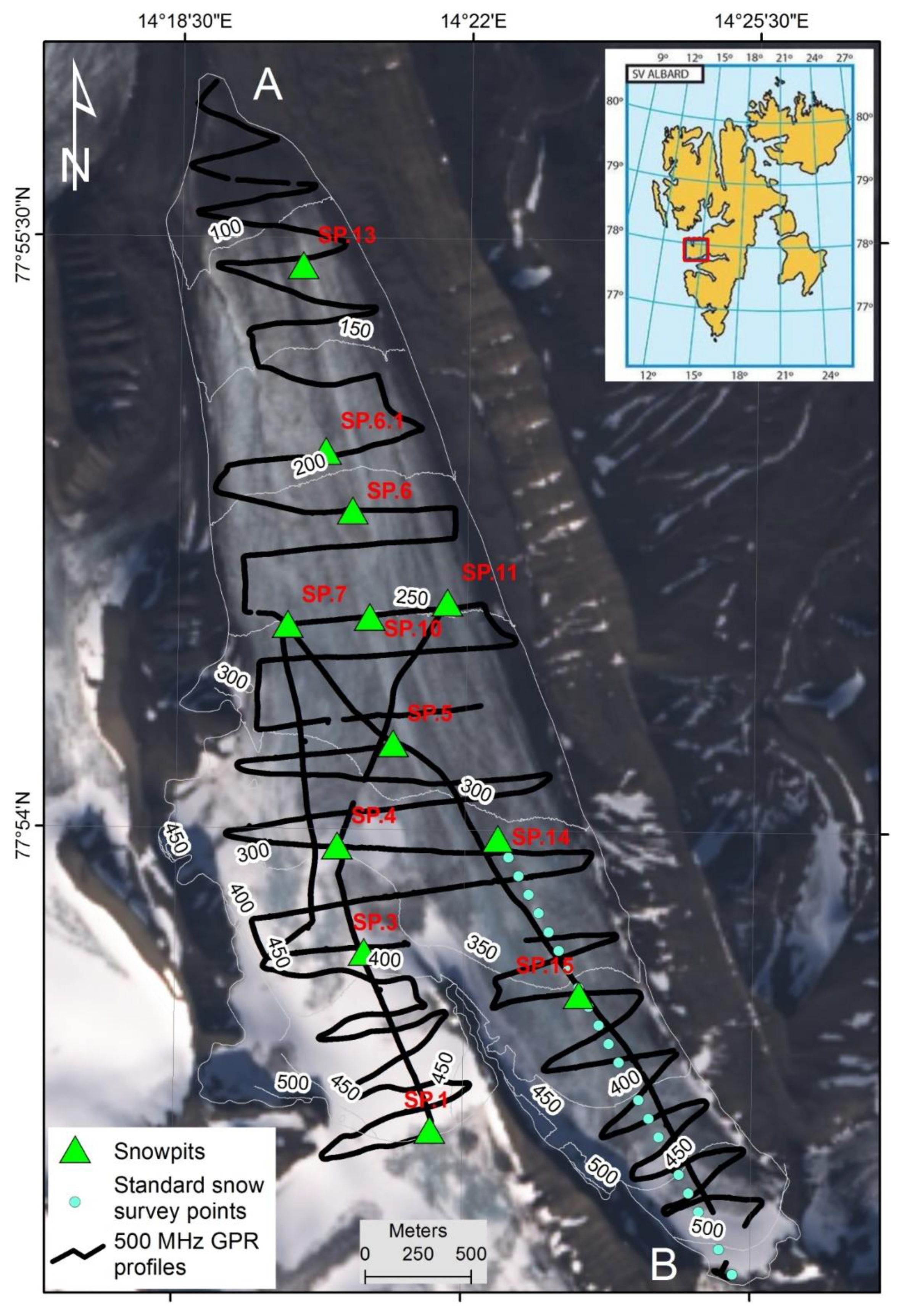
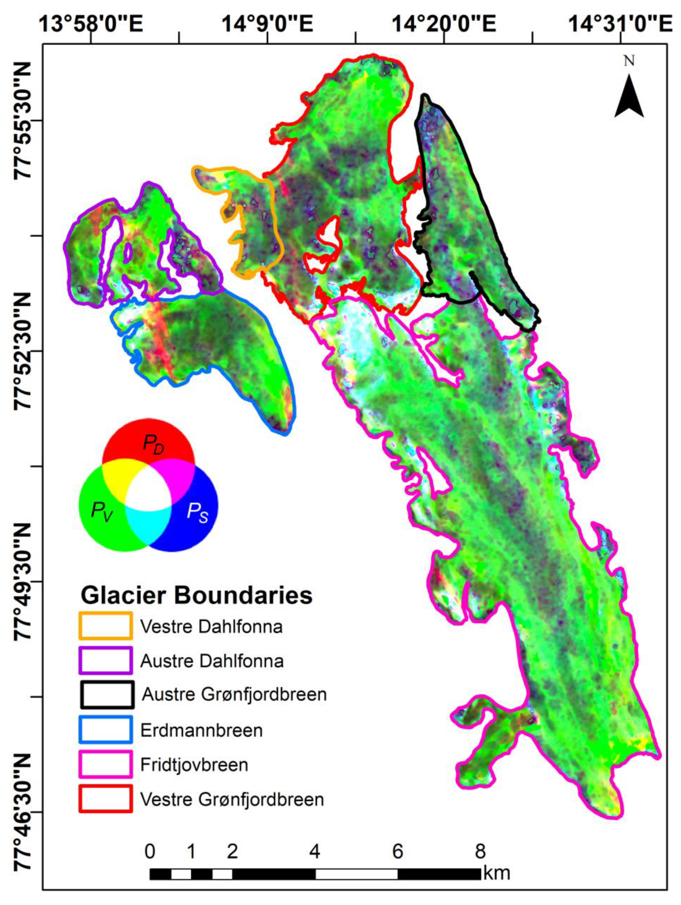
2. Study Area
3. Data Used
3.1. GPR Data and Snow Measurements
3.2. ALOS-2/PALSAR-2 Data
4. Methods
4.1. ALOS-2/PALSAR-2 Data Processing
- Data calibration and matrices formation
- b.
- Orientation angle compensation in [T]
- c.
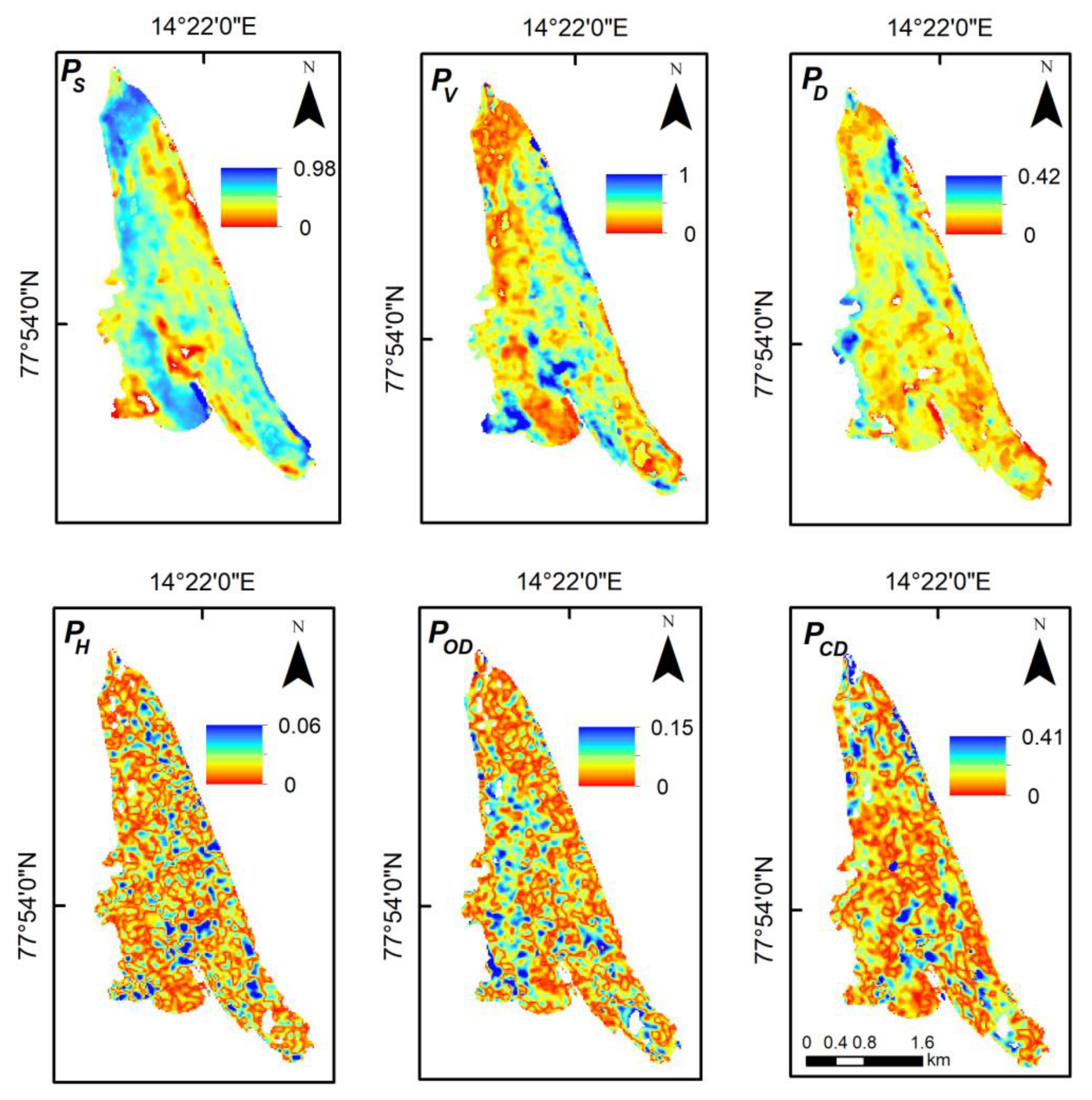
- Six-component scattering matrix power decomposition (6SD)
- d.
- Coherence
4.2. Field-Measured GPR Data Processing and Data Points Reduction
5. Results
5.1. 6SD Interpretation
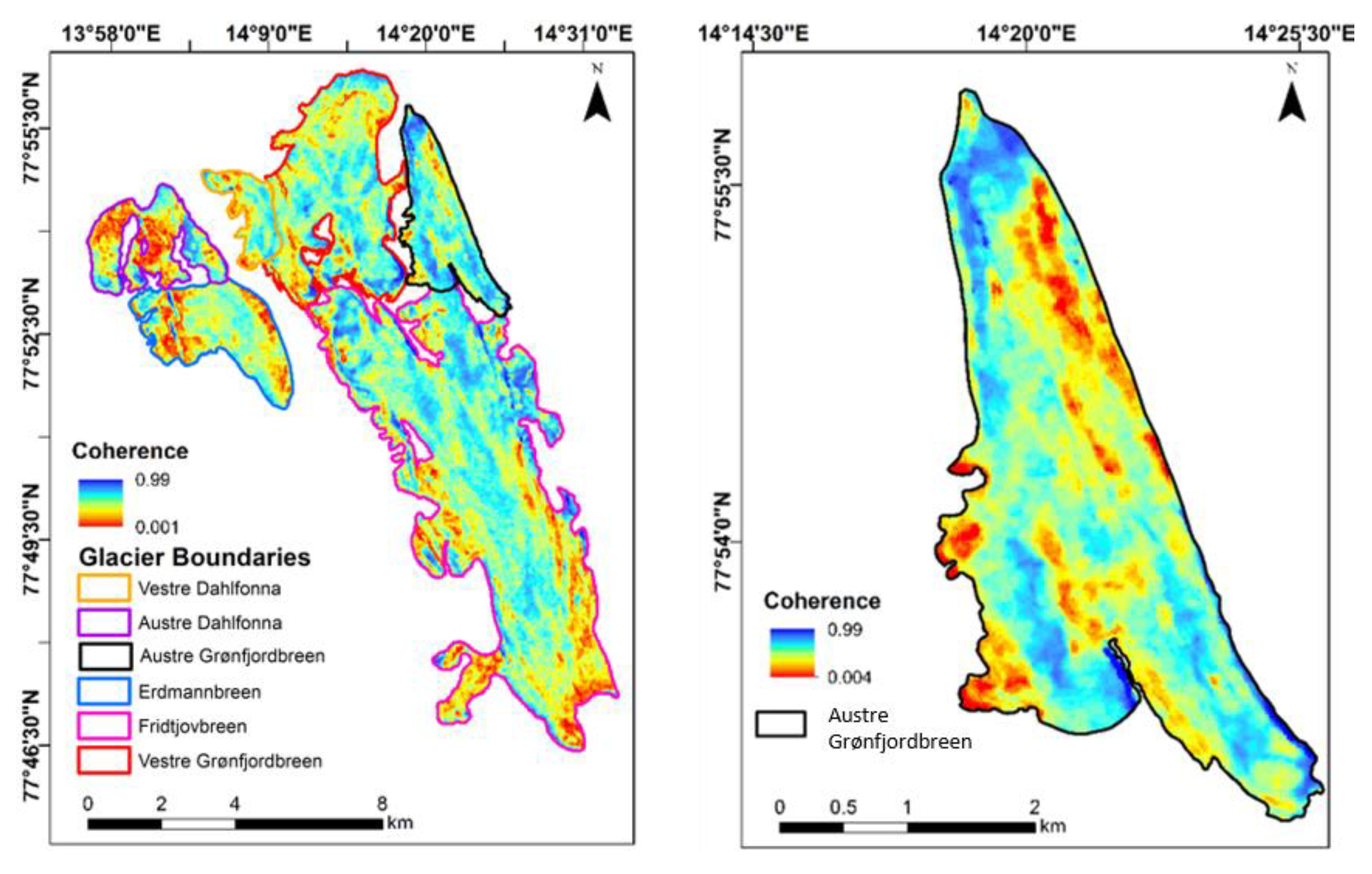
5.2. Coherence Image
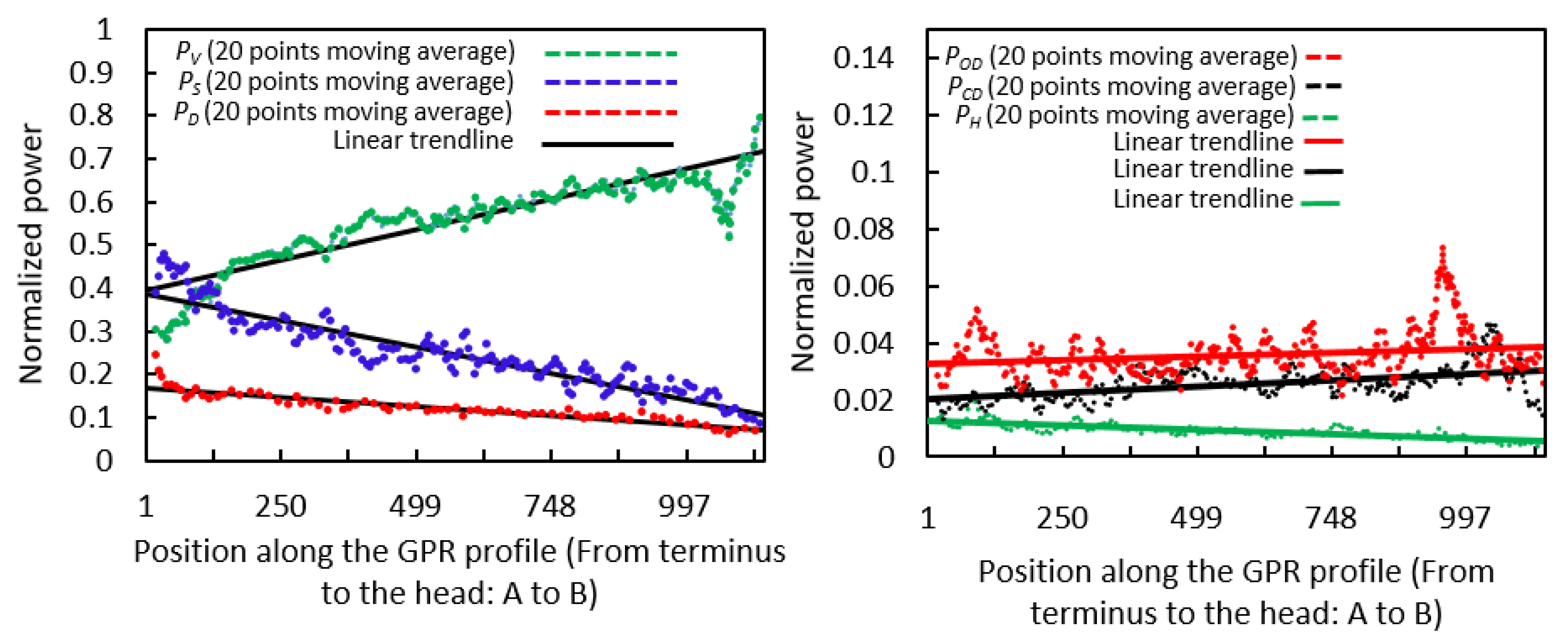
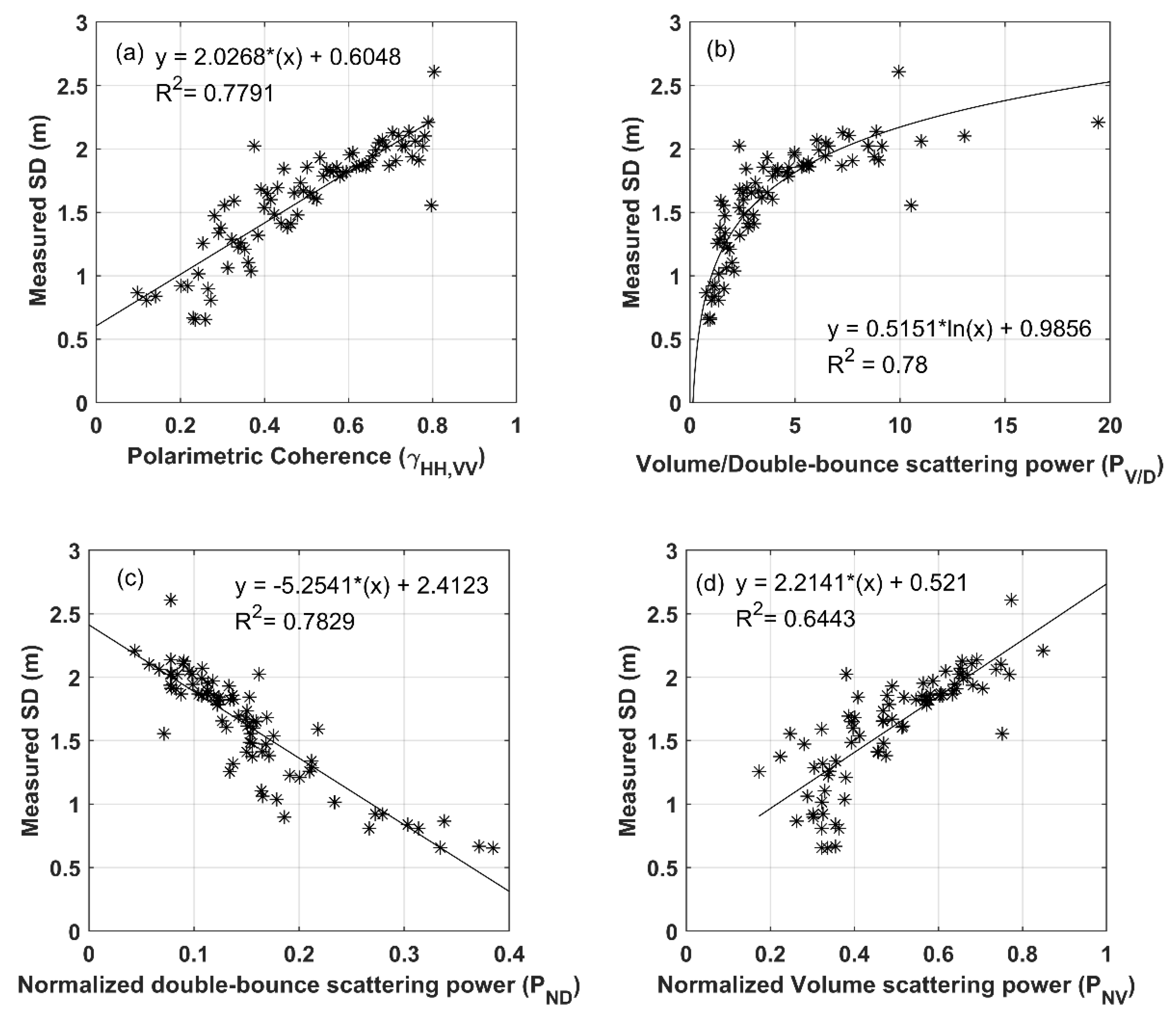
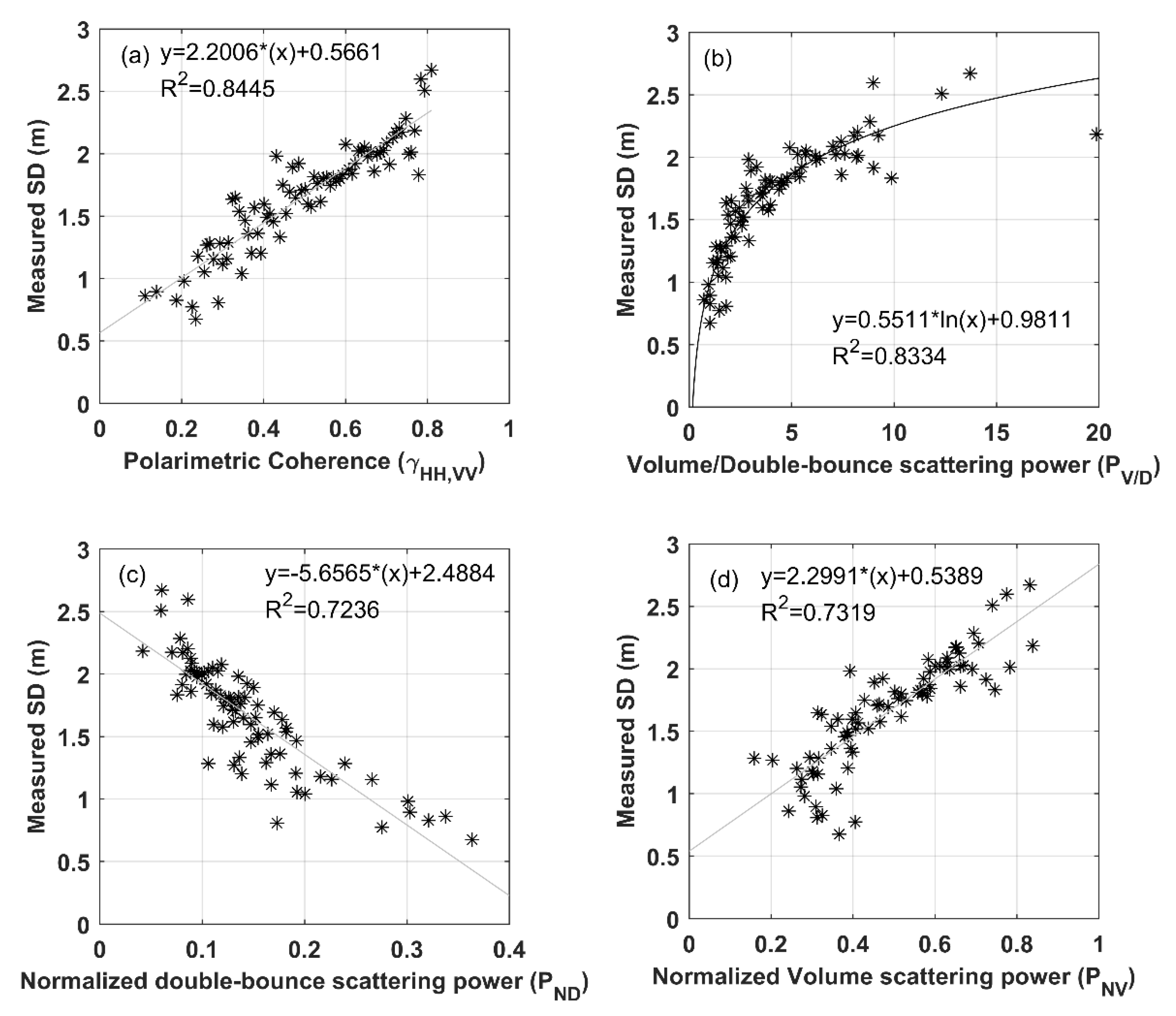
5.3. Behaviour of Polarimetric Parameters with Snow Depth
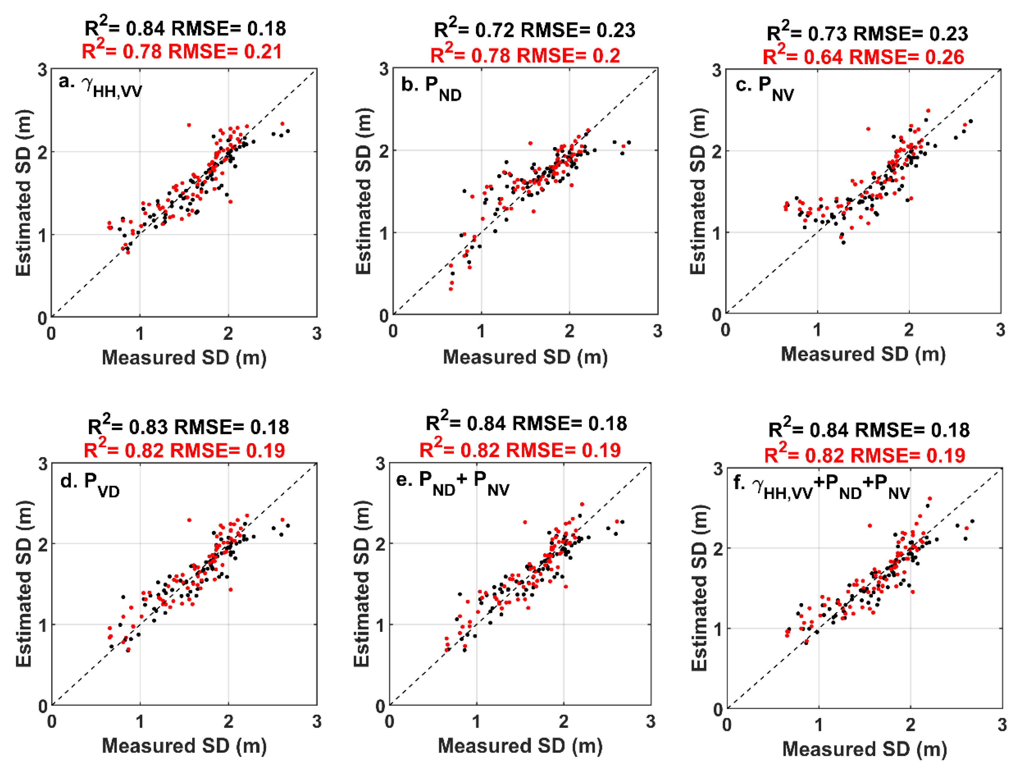
5.4. Inversion and Validation
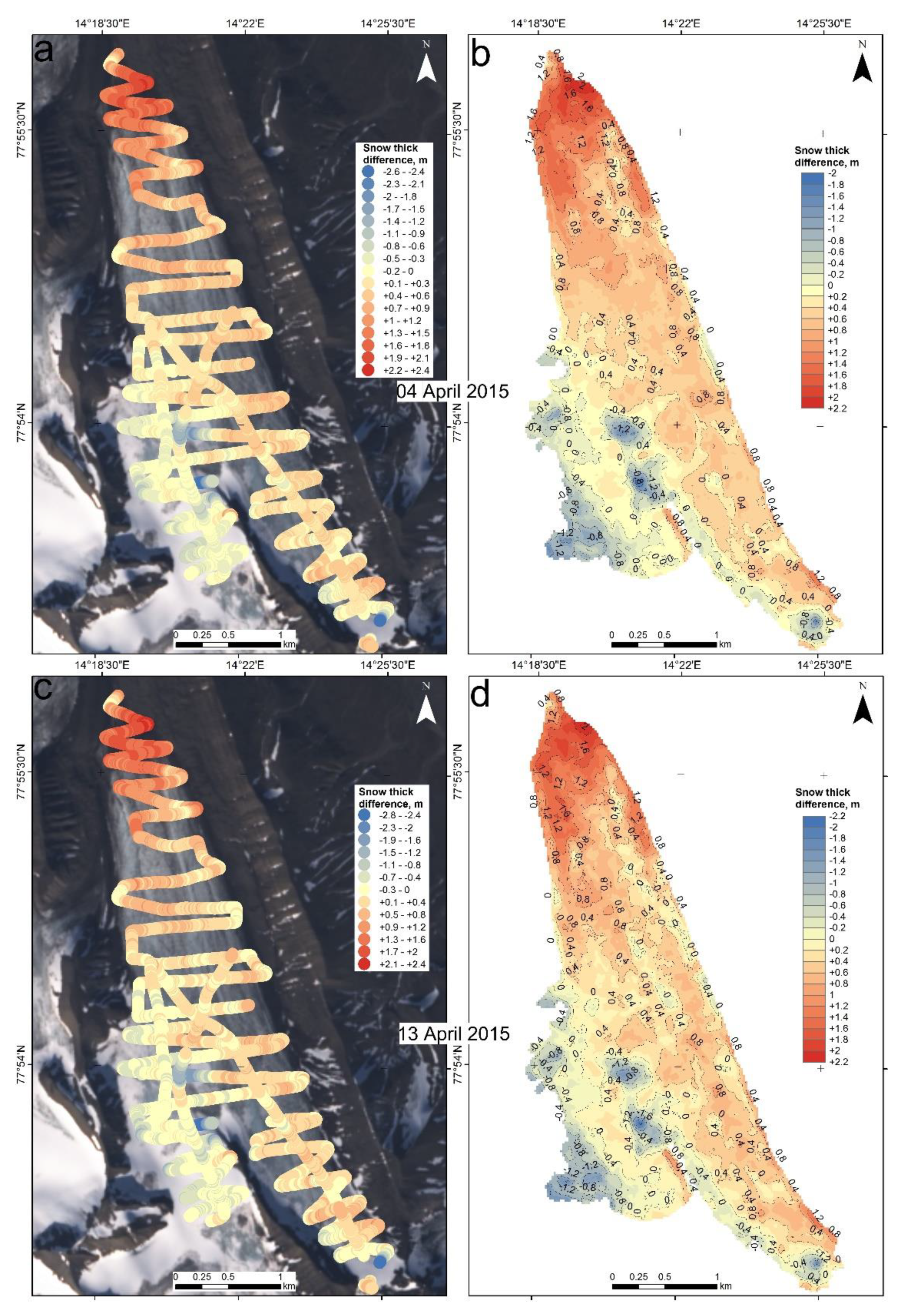
5.5. Comparison SAR and GPR-Based SD and Differences
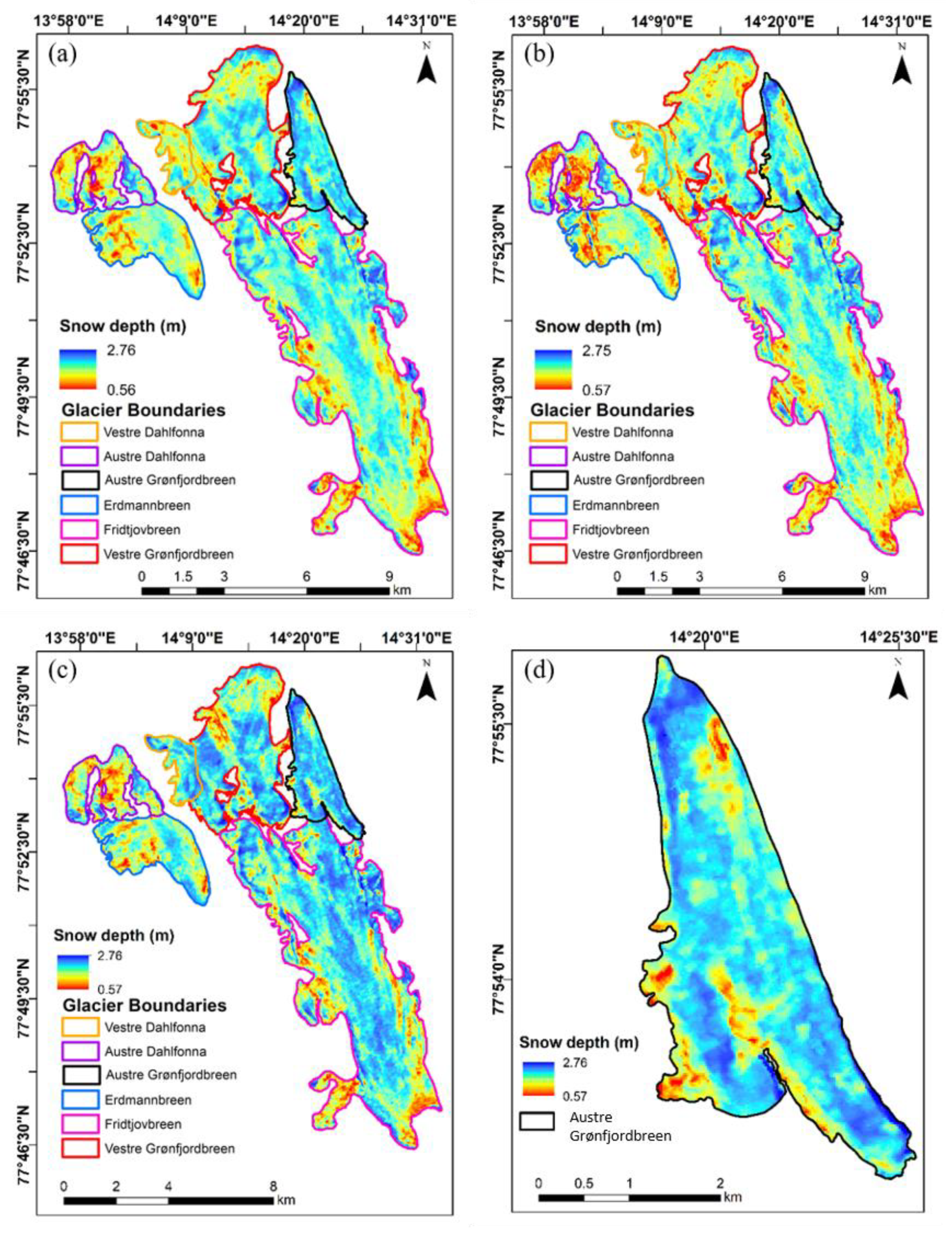
5.6. Spatial and Temporal Variability in Snowpack Depth
6. Conclusions
Author Contributions
Funding
Acknowledgments
Conflicts of Interest
References
- Hill, D.F.; Burakowski, E.A.; Crumley, R.L.; Keon, J.; Hu, J.M.; Arendt, A.A.; Jones, K.W.; Wolken, G.J. Converting snow depth to snow water equivalent using climatological variables. Cryosphere 2019, 13, 1767–1784. [Google Scholar] [CrossRef] [Green Version]
- Janetti, E.B.; Gorni, E.; Sovilla, B.; Bocchiola, D. Regional snow-depth estimates for avalanche calculations using a two-dimensional model with snow entrainment. Ann. Glaciol. 2008, 49, 63–70. [Google Scholar] [CrossRef]
- Gray, D.M. Snow Accumulation and Distribution. In Presented at “Modeling Snow Cover Runoff” U.S.; Army Cold Regions Research and Engineering Laboratory: Hanover, NH, USA, 1978; pp. 1–31. [Google Scholar]
- Grünewald, T.; Bühler, Y.; Lehning, M. Elevation dependency of mountain snow depth. Cryosphere 2014, 8, 2381–2394. [Google Scholar] [CrossRef] [Green Version]
- Ahlamnn, H.W. Scientific results of the Swedish−Norwegian Arctic Expedition in the summer of 1931, Part VIII. Geogr. Ann. 1933, 15, 161–216. [Google Scholar] [CrossRef]
- Mikhaliov, V.S.; Singer, E.M. Feeding of glaciers. In Oledinienie Szpicbergena (Svalbarda); Troickij, L.S., Zinger, E.M., Koriakin, W.S., Markin, W.A., Mihalev, W.I., Eds.; Nauka: Moskwa, Russia, 1975; pp. 106–152. (In Russian) [Google Scholar]
- Koryakin, V.S.; Krenke, A.N.; Tareeva, A.M. Calculated accumulation at equilibrium line altitude. In Glaciologia Shpicbergena; Kotljakov, B.M., Ed.; Nauka: Moskva, Russia, 1985; pp. 54–61. (In Russian) [Google Scholar]
- Lavrentiev, I.I.; Kutuzov, S.S.; Glazovsky, A.F.; Macheret, Y.Y.; Osokin, N.I.; Sosnovsky, A.V.; Chernov, R.A.; Cherniakov, G.A. Snow thickness on Austre Grønfjordbreen, Svalbard, from radar measurements and standard snow surveys. Led Sneg. Ice Snow 2018, 58, 5–20. (In Russian) [Google Scholar] [CrossRef]
- Grabiec, M.; Puczko, D.; Budzik, T.; Gajek, G. Snow distribution patterns on Svalbard glaciers derived from radio-echo soundings. Pol. Polar Res. 2011, 32, 393–421. [Google Scholar] [CrossRef] [Green Version]
- Gallet, J.C.; Björkman, M.P.; Borstad, C.P.; Hodson, A.J.; Jacobi, H.W.; Larose, C.; Luks, B.; Spolaor, A.; Schuler, T.V.; Urazgildeeva, A.; et al. Snow Research in Svalbard: Current Status and Knowledge Gaps. In State of Environmental Science in Svalbard (SESS) Report 2018; Available online: https://sios-svalbard.org/sites/sios-svalbard.org/files/common/SESS_2018_03_SnowResearch.pdf (accessed on 30 September 2019).
- Grabiec, M.; Leszkiewicz, J.; Głowacki, P.; Jania, J. Distribution of snow accumulation on some glaciers of Spitsbergen. Pol. Polar Res. 2006, 27, 309–326. [Google Scholar]
- Möller, M.; Möller, R. Snow cover variability across glaciers in Nordenskiöldland (Svalbard) from point measurements in 2014–2016. Earth Syst. Sci. Data Discuss 2019. [Google Scholar] [CrossRef]
- Singh, G.; Verma, A.; Kumar, S.; Ganju, A.; Yamaguchi, Y.; Kulkarni, A.V. Snowpack density retrieval using fully polarimetric TerraSAR-X data in the Himalayas. IEEE Trans. Geosci. Remote Sens. 2017, 55, 6320–6329. [Google Scholar] [CrossRef]
- Singh, G.; Venkataraman, G.; Yamaguchi, Y.; Park, S.E. Capability assessment of fully polarimetric ALOS PALSAR data to discriminate wet snow from other targets. IEEE Trans. Geosci. Remote Sens. 2014, 52, 1177–1196. [Google Scholar] [CrossRef]
- Singh, G.; Venkatraman, G. Snow wetness mapping using advanced synthetic aperture radar data. J. Appl. Remote Sens. 2007, 1, 013521. [Google Scholar] [CrossRef]
- Lievens, H.; Demuzere, M.; Marshall, H.P.; Reichle, R.H.; Brucker, L.; Brangers, I.; De Rosnay, P.; Dumont, M.; Girotto, M.; Immerzeel, W.W.; et al. Snow depth variability in the Northern Hemisphere mountains observed from space. Nat. Commun. 2019, 10, 4629. [Google Scholar] [CrossRef] [PubMed]
- Tsai, Y.L.S.; Dietz, A.; Oppelt, N.; Kuenzer, C. Remote Sensing of Snow Cover Using Spaceborne SAR: A Review. Remote Sens. 2019, 11, 1456. [Google Scholar] [CrossRef] [Green Version]
- Surendar, M.; Bhattacharya, A.; Singh, G.; Yamaguchi, Y. Estimation of snow surface dielectric constant from polarimetric SAR data. IEEE J. Sel. Top. Appl. Remote Sens. 2017, 10, 211–218. [Google Scholar]
- Surendar, M.; Bhattacharya, A.; Singh, G.; Yamaguchi, Y.G. Venkataraman Estimation of snow density using full-polarimetric Synthetic Aperture Radar (SAR) data. Phys. Chem. Earth 2015, 83, 156–165. [Google Scholar] [CrossRef]
- Goodison, B.E. Determination of areal snow water equivalent on the Canadian Prairies using passive microwave satellite data. In Proceedings of the 12th Canadian Symposium on Remote Sensing Geoscience and Remote Sensing Symposium, Vancouver, Canada, 10–14 July 1989; Volume 3, pp. 1243–1246. [Google Scholar]
- Foster, J. Comparison of snow mass estimates from a prototype passive microwave snow algorithm, a revised algorithm and a snow depth climatology. Remote Sens. Environ. 1997, 62, 132–142. [Google Scholar] [CrossRef]
- Che, T.; Li, X.; Jin, R.; Armstrong, R.; Zhang, T. Snow depth derived from passive microwave remote-sensing data in China. Ann. Glaciol. 2008, 49, 145–154. [Google Scholar] [CrossRef] [Green Version]
- Singh, G.; Venkataraman, G. Snow density estimation using Polarimitric ASAR data. In Proceedings of the 2009 IEEE International Geoscience and Remote Sensing Symposium, Cape Town, South Africa, 12–17 July 2009; Volume 2, pp. 630–633. [Google Scholar]
- Surendar, M.; Bhattacharya, A.; Singh, G.; Yamaguchi, Y.; Venkataraman, G. Development of a snow wetness inversion algorithm using polarimetric scattering power decomposition model. Int. J. Appl. Earth Observ. Geoinf. 2015, 42, 65–75. [Google Scholar] [CrossRef]
- Leinss, S.; Parrella, G.; Hajnsek, I. Snow height determination by polarimetric phase differences in X-band SAR data. IEEE J. Sel. Top. Appl. Earth Observ. Remote Sens. 2014, 7, 3794–3810. [Google Scholar] [CrossRef] [Green Version]
- Patil, A.; Singh, G.; Rudiger, C. Estimation of snow water equivalent using Sentinel SAR Data in the Indian Himalaya. In Proceedings of the IGARSS 2018—2018 IEEE International Geoscience and Remote Sensing Symposium, Valencia, Spain, 22–27 July 2018; pp. 2789–2792. [Google Scholar]
- Singh, G.; Yamaguchi, Y.; Park, S.E. Evaluation of modified four-component scattering power decomposition method over highly rugged glaciated terrain. Geocarto Int. 2012, 27, 139–151. [Google Scholar] [CrossRef]
- Yamaguchi, Y.; Sato, A.; Boerner, W.M.; Sato, R.; Yamada, H. Four component scattering power decomposition with rotation of coherency matrix. IEEE Trans. Geosci. Remote Sens. 2011, 49, 2251–2258. [Google Scholar] [CrossRef]
- Has Fridtjovbreen, Svalbard Surged for the Last Time? Available online: https://blogs.agu.org/fromaglaciersperspective/2016/12/20/fridtjovbreen-svalbard-surged-last-time/ (accessed on 9 November 2019).
- Kulnitsky, L.M.; Gofman, P.A.; Tokarev, M.Y. Mathematical processing of georadar data in the RADEXPRO system. Razvedka i okhrana nedr. Explor. Protect. Miner. Resour. 2001, 3, 6–11. (In Russian) [Google Scholar]
- Looyenga, H. Dielectric constants of heterogeneous mixtures. Physica 1965, 31, 401–406. [Google Scholar] [CrossRef]
- About ALOS-2. Available online: http://en.alos-pasco.com/alos-2/ (accessed on 9 November 2019).
- Lee, J.S.; Pottier, E. Polarimetric Radar Imaging: From Basics to Applications; CRC Press/Taylor & Francis: Boca Raton, FL, USA, 2009. [Google Scholar]
- Singh, G.; Venkataraman, G. Application of incoherent target decomposition theorems to classify snow cover over the Himalayan region. Int. J. Remote Sens. 2012, 33, 4161–4177. [Google Scholar] [CrossRef]
- Yamaguchi, Y. Radar Polarimetry from Basics to Applications; IEICE: Tokyo, Japan, 2007; p. 182. (In Japanese) [Google Scholar]
- Freeman, A.; Durden, S. A three-component scattering model for polarimetric SAR data. IEEE Trans. Geosci. Remote Sens. 1998, 36, 963–973. [Google Scholar] [CrossRef] [Green Version]
- Singh, G.; Yamaguchi, Y.; Park, S.E. Utilization of four-component scattering power decomposition method for glaciated terrain classification using fully polarimetric PALSAR data. Geocarto Int. 2011, 26, 377–389. [Google Scholar] [CrossRef]
- Yamaguchi, Y.; Moriyama, T.; Ishido, M.; Yamada, H. Four component scattering model for polarimetric SAR image decomposition. IEEE Trans. Geosci. Remote Sens. 2005, 43, 1699–1706. [Google Scholar] [CrossRef]
- Sato, A.; Yamaguchi, Y.; Singh, G.; Park, S.E. Four-component scattering power decomposition with extended volume scattering model. IEEE Geosci. Remote Sens. Lett. 2011, 9, 166–170. [Google Scholar] [CrossRef]
- Singh, G.; Yamaguchi, Y.; Park, S.E. General four-component scattering power decomposition with unitary transformation of coherency matrix. IEEE Trans. Geosci. Remote Sens. 2013, 51, 3014–3022. [Google Scholar] [CrossRef]
- Singh, G.; Yamaguchi, Y. Model-Based Six-Component Scattering Matrix Power Decomposition. IEEE Trans. Geosci. Remote Sens. 2018, 56, 5687–5704. [Google Scholar] [CrossRef]
- Arbia, G. The Use of GIS in Spatial Statistical Surveys. Int. Stat. Rev. 1993, 61, 339–359. [Google Scholar] [CrossRef]
- Hall, D. Remote sensing of snow and ice using imaging radar. In Principle and Application of Imaging Radar, Manual of Remote Sensing, 3rd ed.; Henderson, F., Lewis, A., Eds.; John Wiley & Sons Ltd.: Hoboken, NJ, USA, 1998; Volume 2, pp. 677–698. [Google Scholar]
- Shi, J.; Dozier, J. Estimation of snow water equivalence using SIR-C/X-SAR. I. Inferring snow density and subsurface properties. IEEE Trans. Geosci. Remote Sens. 2000, 38, 2465–2474. [Google Scholar] [CrossRef] [Green Version]


| Date of Acquisition | Polarization | Off-Nadir Angle | Range Resolution | Azimuth Resolution | Level of Data Product | Observation Mode/Orbit Pass |
|---|---|---|---|---|---|---|
| 4 April 2015 | Quad | 32.7° | 5.1 m | 4.3 m | SLC, Level 1.1 | Stripmap/Ascending |
| 13 April 2015 | Quad | 30.4° | ||||
| 15 May 2015 | Quad | 25.0° |
| Parameters | COH | ||||||
|---|---|---|---|---|---|---|---|
| Trained G1 Validated G2 | R2 | 0.84 | 0.72 | 0.73 | 0.83 | 0.84 | 0.84 |
| RMSE (m) | 0.18 | 0.23 | 0.23 | 0.18 | 0.18 | 0.18 | |
| Trained G2 Validate G1 | R2 | 0.78 | 0.78 | 0.64 | 0.78 | 0.82 | 0.82 |
| RMSE (m) | 0.21 | 0.20 | 0.26 | 0.21 | 0.19 | 0.19 | |
© 2019 by the authors. Licensee MDPI, Basel, Switzerland. This article is an open access article distributed under the terms and conditions of the Creative Commons Attribution (CC BY) license (http://creativecommons.org/licenses/by/4.0/).
Share and Cite
Singh, G.; Lavrentiev, I.I.; Glazovsky, A.F.; Patil, A.; Mohanty, S.; Khromova, T.E.; Nosenko, G.; Sosnovskiy, A.; Arigony-Neto, J. Retrieval of Spatial and Temporal Variability in Snowpack Depth over Glaciers in Svalbard Using GPR and Spaceborne POLSAR Measurements. Water 2020, 12, 21. https://doi.org/10.3390/w12010021
Singh G, Lavrentiev II, Glazovsky AF, Patil A, Mohanty S, Khromova TE, Nosenko G, Sosnovskiy A, Arigony-Neto J. Retrieval of Spatial and Temporal Variability in Snowpack Depth over Glaciers in Svalbard Using GPR and Spaceborne POLSAR Measurements. Water. 2020; 12(1):21. https://doi.org/10.3390/w12010021
Chicago/Turabian StyleSingh, Gulab, Ivan I. Lavrentiev, Andrey F. Glazovsky, Akshay Patil, Shradha Mohanty, Tatiana E. Khromova, Gennady Nosenko, Aleksandr Sosnovskiy, and Jorge Arigony-Neto. 2020. "Retrieval of Spatial and Temporal Variability in Snowpack Depth over Glaciers in Svalbard Using GPR and Spaceborne POLSAR Measurements" Water 12, no. 1: 21. https://doi.org/10.3390/w12010021