The Use of a Microscale Physical Model to Simulate Bankfull Discharge in the Lower Reaches of the Yellow River


1
College of Water Resources and Civil Engineering, China Agricultural University, Beijing 100083, China
2
Agriculture, Forestry and Water Affairs Bureau of the National Linyi Economic & Technological Development Area, Linyi 276000, China
3
China Water Resources Bei Fang Investigation, Design & Research CO.LTD, Tianjin 300222, China
*
Author to whom correspondence should be addressed.
Water 2020, 12(1), 13; https://doi.org/10.3390/w12010013
Submission received: 8 November 2019
/
Revised: 13 December 2019
/
Accepted: 17 December 2019
/
Published: 19 December 2019
(This article belongs to the Special Issue Physical Modelling in Hydraulics Engineering)
Abstract
:Microscale physical models (MSPMs) were once widely used in flood planning in large basins. They fell out of favor but are now being used again. This paper explores the benefits of using such a model for understanding a flood problem on the Lower Yellow River (LYR). We constructed an indoor MSPM of a nearly 800-km reach of the LYR. The model had different scales in the longitudinal, transverse, and vertical directions, and we adjusted the slope of the model. Meanwhile, a real-time water level monitoring system and an automatic flow control system were built on the MSPM to automatically control hydrodynamic testing. Through several discharge experiments, bankfull discharge for multiple MSPM sections was obtained and compared with measured data from the corresponding hydrological section of the prototype during the early flood season of 2016. The comparison demonstrated good linear correlation. The analysis of model similarity showed that although there was some deviation in gravity similarity between the MSPM and the prototype, the model discharge scale derived from resistance similarity adequately described the relationship between the model and the prototype bankfull discharge. Further analysis of the relationship between the model and the prototype bankfull discharge revealed that a split-line line may be better than a single regression line. A MSPM could reproduce the bankfull discharge of the LYR with the nearly 800-km reach in the laboratory which is impossible for a small distortion rate physical model, and obtain a result close to that of the assimilated numerical model.
1. Introduction
Microscale physical models (MSPMs) are extremely small-scale physical river models that can produce quick answers to river engineering problems [1]. Multiyear river physical model experiments have been carried out for over a century and play an important role in studying river regulation. Compared with prototype observation and numerical simulation method, river physical model experiments have the advantages of being able to simulate the past and future flooding events, and directly reflect the constitutive relation between the water flow and the river. Thus, it has become an important tool for river regulation [2].
The U.S. Army Corps of Engineers (USACE) published a patented technology known as Micro Hydraulic Modeling Technology [3] in 1997, and successfully applied it to the Mississippi River to deal with various sediment problems. Maynord [1] used the results of a USACE Research and Development Program-funded evaluation to determine the capabilities and limitations of the MSPM. They found that the model can not only predict the flow pattern trends of river training structure under the influence of navigation and environment, but also explain the river training activities to nonhydraulic experts. Additionally, these benefits provide a timely assessment of navigation plans. Later, the development and application of MSPMs continued, but the USACE began to dispute their use. Consequently, they evaluated MSPMs to determine their capabilities and limitations. Gaines et al. [4] described such an evaluation plan. Smith [2], Davies [5], and Gabriel Echávez et al. [6] evaluated their predictive capacity. They confirmed MSPMs can predict the effect of river engineering to replicate flow processes in the prototype.
At present, the river models are dominated by distorted scale in practice. Its main advantage is that it can achieve roughness satisfying resistance similarity, while it is technically impossible in a normal scale physical model with the same horizontal and vertical scale. Research on modeled water flow and sediment movement after distortion has also attracted the attention of many scholars. In 2002, Maynord [7] measured surface velocity using the Vicksburg model. Velocity comparisons showed that flow distribution in the Vicksburg Front MSPM was not similar to the prototype, likely due to model distortions. Li [8] conducted a preliminary exploration of the experimental techniques and theoretical basis of micro-river models in 2012. He proposed the selection of MSPM scale, a requirement for water flow resistance similarity, and a specific method for roughness adjustment. This method will be helpful to study the regulation of the Yangtze River waterway system. Mao et al. [9] analyzed the influence of channel sand excavation on riverbed evolution by using a MSPM that had a large distortion rate of up to 36.67. The results indicated that the MSPM could be used for qualitative analysis. However, the effects of distortion on river hydrodynamics need further assessment.
Research on floodplain governance in the Lower Yellow River (LYR) is related to the national economy and human livelihoods. With economic development, the production and land area for nearly 1.9 million people living in the floodplain has constricted river flood space [10]. The contradiction between flood control security and beach development is becoming more and more prominent. Bankfull discharge in the river section represents an initial flood stage and is considered to be an important indicator for studying river morphology, flood management, and its ecological impacts. The simulation of bankfull discharge provides a practical tool for flood risk management. Although numerical models are capable and have been well-developed, they only can be used after the calibration and verification of measured data. In our previous work, the calibrated numerical model still cannot obtain accurate results in the entire calculation domain due to the uncertainty of the numerical discrete method, parameter determination, and boundary generalization in solving the Navier–Stocks equation [11,12]. In addition, physical models can replace the longer period of the prototype with shorter indoor testing time because of time scale [13]. However, it is impossible to construct a normal scale or small distortion rate physical model of the LYR with a length of hundreds of kilometers in the laboratory. It is worthwhile to try to reproduce multisection bankfull discharge in MSPMs.
Hence, the purpose of this paper is as follows: (1) to simulate bankfull discharge in the LYR, which marks the condition of incipient flooding and aids in flood risk management, (2) to evaluate the impacts of three-dimensional distortion on hydrodynamic and similarity trends, and (3) to study bankfull discharge along a long river using a MSPM. Quantitative analysis was performed to describe how the MSPM can help solve river engineering problems.
2. Materials and Methods
2.1. Description of the MSPM
The MSPM was constructed in a laboratory to mimic the nearly 800-km river channel in the LYR. First, we consider the limitations of the laboratory area and the length of the prototype channel. The longitudinal scale λL was determined to be 28,000. If the water depth of the model was too small, it was likely that the Reynolds number was too small, the flow could not be fully turbulent, and measurement accuracy was difficult to guarantee. To maintain a certain water depth, the vertical scale λH was determined to be 50. Finally, the river channel was extended 20 times horizontally along the centerline to make the model size suitable for hydrodynamic experiments, so the transverse scale λB was 1400. The transverse and longitudinal distortions are 28 and 560, respectively. In addition, the model had a total length of 27.38 m. The average slope was 1/250 according to the preliminary similarity analysis.
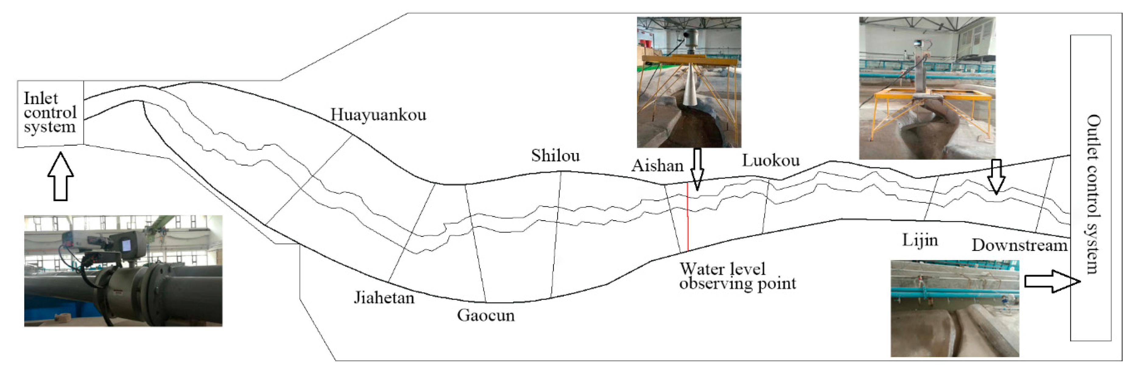
The cross-section data was generalized based on the 1:100,000 dataset from the National Earth System Science Data Center, National Science and Technology Infrastructure of China, and corrected by cross-section data measured in 2013 before the flood season. Furthermore, we identified 57 important river sections, including Huayuankou (HYK), Jiahetan (JHT), Gaocun (GC), Shilou (SL), Aishan (AS), Sunkou (SK), Luokou (LK), and Lijin (LJ) (Figure 1). After selecting the datum point coordinate at the laboratory, the position coordinates and elevation of each section in the model were determined. The section board was drawn according to the coordinate and elevation values for each section. Then, the section boards were attached at the fix points referring to construction reference line. At last, the section boards were filled with cement and a smooth transition was ensured. The upper boundary of the model simulation range was the Dongxiayuan (DXY) section, and the lower boundary was the Branch 3 section. The indoor MSPM plane view is shown in Figure 1.
2.2. Model Automatic Control and Monitoring System
Automatic inlet flow discharge and outlet water level (tidal) control took place in the MSPM. The inlet of the model was equipped with an automatic flow control system using a variable frequency flow meter and camera combination to ensure the system released the specified water flow. This system controlled discharge in manual, feedback, and documentation modes. The tail water automatic control system for the downstream estuary consisted of six pumps and a needle water level gauge. Three pumps were used to pump water from the tail water pool to the drainage channel, while the other three pumped water in the opposite direction. The discharge ranges of the pumps were strictly calibrated. The water level in the tail pool was monitored by the needle water level gauge and displayed on the computer. During operation, the tail water control system combined different pump numbers to achieve a specified discharge and produced a specified tidal water level process. The Yellow River Estuary is a microtidal estuary. The tidal range is saddle-shaped along the delta coast, with an average tidal range of 1.1 to 1.5 m. The tidal reach is extremely short, and the range of the estuary influenced by tidal is 10–20 km [14]. According to the longitudinal scale λL of the MSPM, the influenced range of the model is 0.357–0.714 m away from the estuary. The farthest section influenced by tidal is Qing-7 section, 0.7608 m away from the estuary. As a result, the tide has no influence on the bankfull discharge of typical sections above LJ.
The water level monitoring system included the radar gauge and data acquisition program that automatically saved recorded water levels at the observation point (see in Figure 1). When the model operated at a constant flow, the system was also used to determine whether the water level of the section remained constant.
2.3. Measuring Bankfull Discharge
When measuring bankfull discharge, the automatic flow control system released water through a constant small discharge. Meanwhile, radar water level and needle water level gauge readings were observed. After the water level of the gauges stabilized at a certain value, the status of each section was observed. If the water level of one section was equal to its floodplain elevation, the constant small discharge released by the automatic flow control system was the bankfull discharge of that section in the discharge event. Then, discharge was slightly increased by the automatic flow control system and maintained for at least 30 min to reach a steady state in the entire channelization region. The lost discharge to the floodplain was supplemented in later 30-min period. The above steps were repeated to observe the floodplain phenomenon of the section under discharge. Discharge began at 2 L/s, and increased at 0.1 L/s intervals until the bankfull discharge of all typical sections had been recorded. Moreover, we did not record discharge of different sections at the same time in one discharge event. The acquisition of bankfull discharge for each section is in a single discharge event with a constant discharge.
2.4. Adjusting the MSPM Slope
When the prototype and model flow achieved hydrodynamic similarity, a fixed proportional relationship between various physical forces in the water flow was needed. However, it was difficult to require all forces to maintain similar proportions simultaneously. In the distorted scale model, the longitudinal and transverse movements of modeled water flow were similar to the prototype as long as the gravity and resistance similarity were simultaneously satisfied.
If the prototype and model flow met the gravity similarity criterion, the secondary forces in movement were neglected:
where λv represents the velocity scale, λH represents the vertical scale.
Due to river water movement, turbulent resistance plays an important role in addition to gravity. Therefore, gravity and resistance similarity must be satisfied simultaneously during the river model experiment. If the prototype and model flow had resistance similarity, we could use the traditional method of increasing and reducing the roughness coefficient, such as placing wires in the water flow or inserting a wooden sign in the model bed. In addition, it was also possible to adjust the river bed ratio to achieve resistance similarity.
In the normal or distorted scale model experiment, an additional ratio was added to achieve resistance similarity. One of the advantages of using this method to adjust the water flow resistance was to maintain the similarity of the turbulent source structure [8]. The slope scale of a general distorted scale model is written as:
where λJ represents the slope scale, Jp and Jm represent the prototype slope and the model slope, respectively, λL represents the longitudinal scale.
According to the slope adjustment method [8], the slope is artificially adjusted to make the model surface line similar. It is assumed that the model slope is adjusted by m times. At that point, the slope scale of the distorted scale model and the velocity scale are written as:
where m is a multiple of the model slope adjustment to make the model water surface line similar, and λn represents the roughness coefficient scale.
Considering that the MSPM was longer, frictional drag and local resistance had simultaneous effects. At that point, the roughness coefficient of the model needed to be controlled to achieve resistance similarity. For a wide and shallow channel, R = H is generally acceptable. For the convenience of calculation, R in Equation (5) was replaced by H. Considering similar conditions for gravity and resistance of water flow, derived from Equations (1) and (4), we obtain:
Assuming m is equal to 1 (no adjustment to the model slope), the roughness coefficient scale λn = 0.0811. The roughness coefficient np of the prototype channel of the Yellow River was 0.015 [15], so the model roughness coefficient nm was calculated to be 0.185. However, in general, the roughness coefficient of the artificial channel ranged from 0.007 to 0.077 [16], and such large values could not be obtained by the conventional method of increasing the roughness coefficient. Therefore, similarity problems had to be solved by adjusting the slope. When the model was constructed according to the artificial channel’s roughness coefficient range, the model roughness coefficient was set as nm = 0.042, and the value of m that satisfied gravity and turbulence resistance similarity was 0.052. As the average downstream slope of the prototype was 1/7300, the average slope of the model was finally determined as
3. Results
3.1. Cross-Sectional Bankfull Discharge in the MSPM
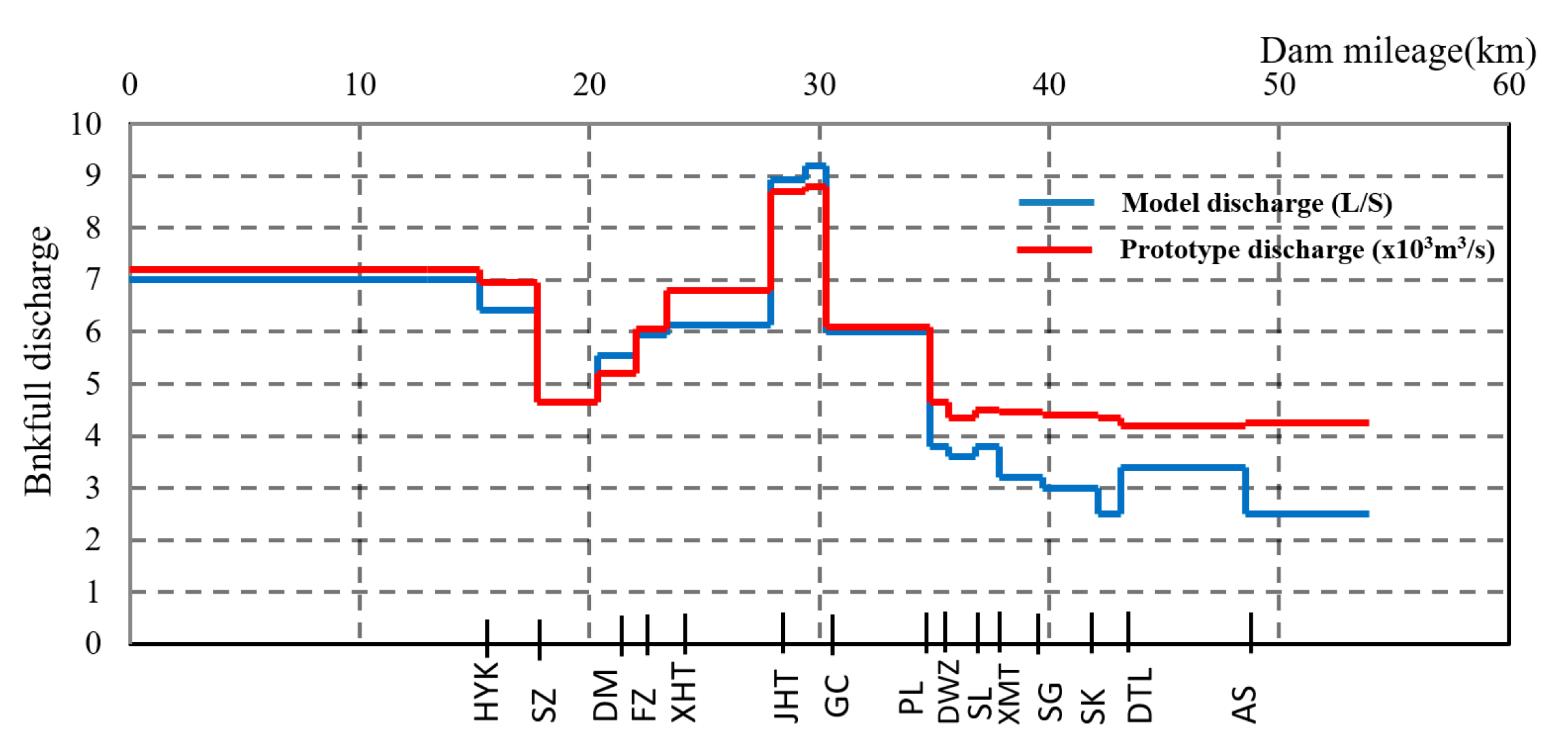
Figure 2 shows the measured bankfull discharge for all sections between the MSPM and the prototype. In the upper reaches above GC, the bankfull discharge was greater than 4500 m3/s in the prototype. According to a consultation report by the Yellow River Institute of Hydraulic Research [17], the main function of Xiaolangdi Reservoir is to retain sediment. Due to sediment retention and the regulation of water and sediment before the flood season, the downstream discharge water is clear with a low sediment concentration, and this part of the river erodes. After a long period of time, the minimum bankfull discharge of upper streams above GC reaches to 4250 m3/s. The bankfull discharge of JHT and GC sections is larger than other sections illustrating that the main channel of these two sections have greater depth and area. In addition, the lower reaches of GC have some sediment retention capacity and cause some sedimentation after a long period. Therefore, bankfull discharges for both the model and prototype are low in the lower reaches of GC. The bankfull discharge of sections in the lower reach of the prototype is less than 4500 m3/s, while that of the MSPM is less than 4.5 L/s (see in Figure 2). In conclusion, there is consistent trend between the prototype and model bankfull discharge.
3.2. Relationship between Model and Prototype Bankfull Discharge
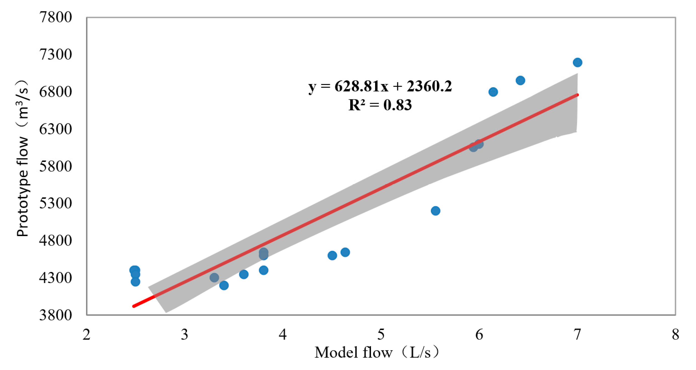
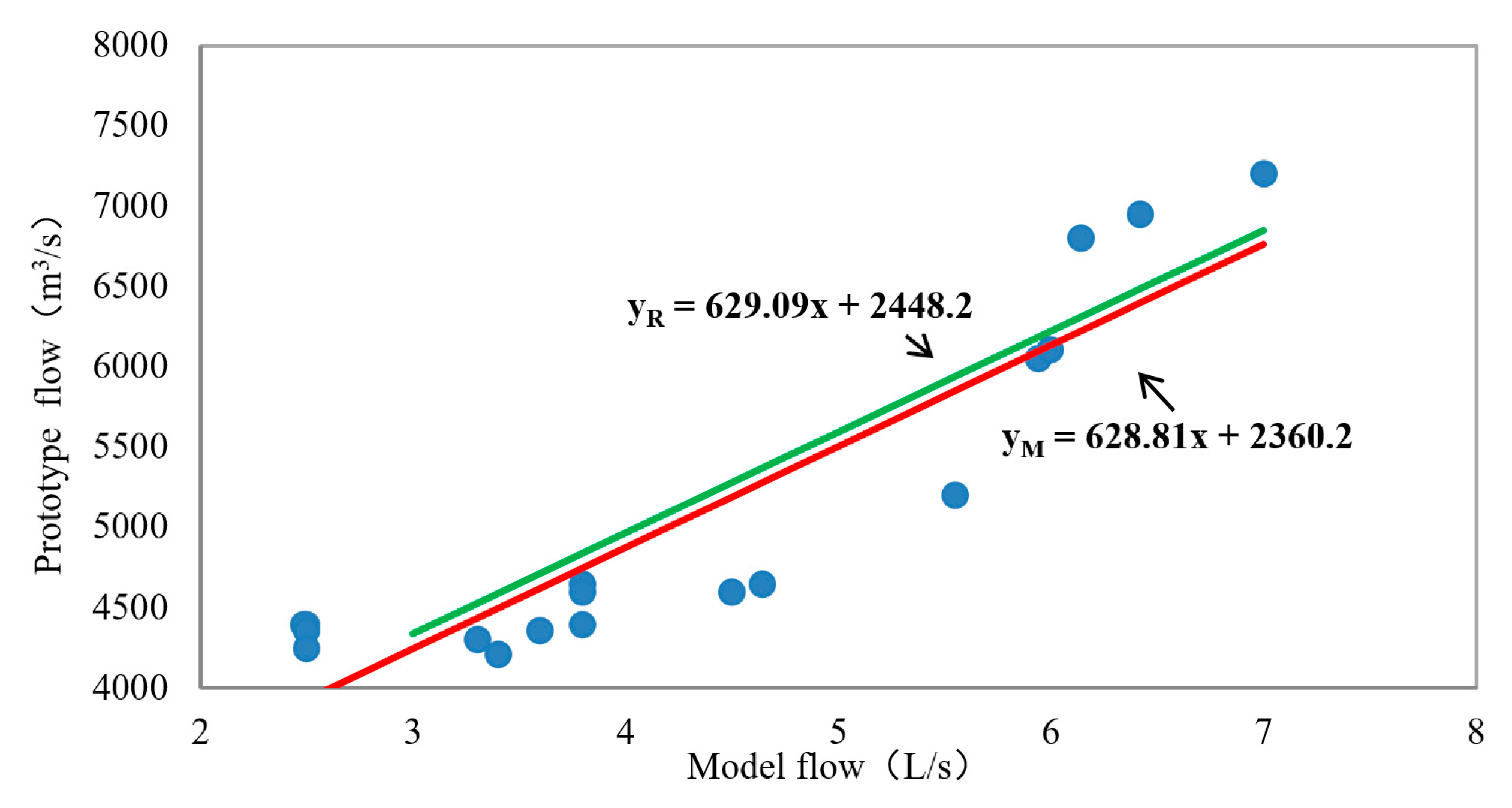
Figure 3 shows the correlation between the MSPM and the prototype bankfull discharge for the same section. In the figure, the model flow was positively correlated with the prototype flow, with a coefficient of determination of R2 = 0.83 which indicated that the model flow is highly linearly correlated with the prototype flow. The slope of the regression line represented the ratio of the prototype flow and model flow in the same section, that is, the flow ratio = 628,810.
3.3. Comparison between Prototype, Physical Model, and Numerical Model Data
The prototype, numerical model data, and other physical model data were chosen to verify the simulation quality of the MSPM. Prototype data were derived from the consultation report by the Yellow River Institute of Hydraulic Research [17]. The cross-section velocity in the prototype was obtained based on the measured water level-velocity relationship [18]. Chen et al. [12] applied a one-dimensional hydrodynamic numerical model and a particle filter-based assimilation model to simulate the variations in water level, discharge, and velocity of each section under multiple nonconstant discharge events. This numerical model was applied to our MSPM. The results show that compared to the traditional numerical model, the assimilation model could effectively update the water level, flow discharge, and roughness coefficient in real time. The boundary condition was set to the measured water discharge at the inlet and a synchronous water level at outlet. The simulation results after assimilation were chosen for comparison. Other physical model data were derived from physical models of Shandong reach, Jinan reach, GC to Yangji reach of the LYR which established by Ruan [19], Li et al. [20], and Dai et al. [21], respectively. As the river channel is too long, it is impossible to construct a normal scale or small distortion rate physical model in the laboratory. No one has ever constructed a physical model of the entire reach of the LYR.
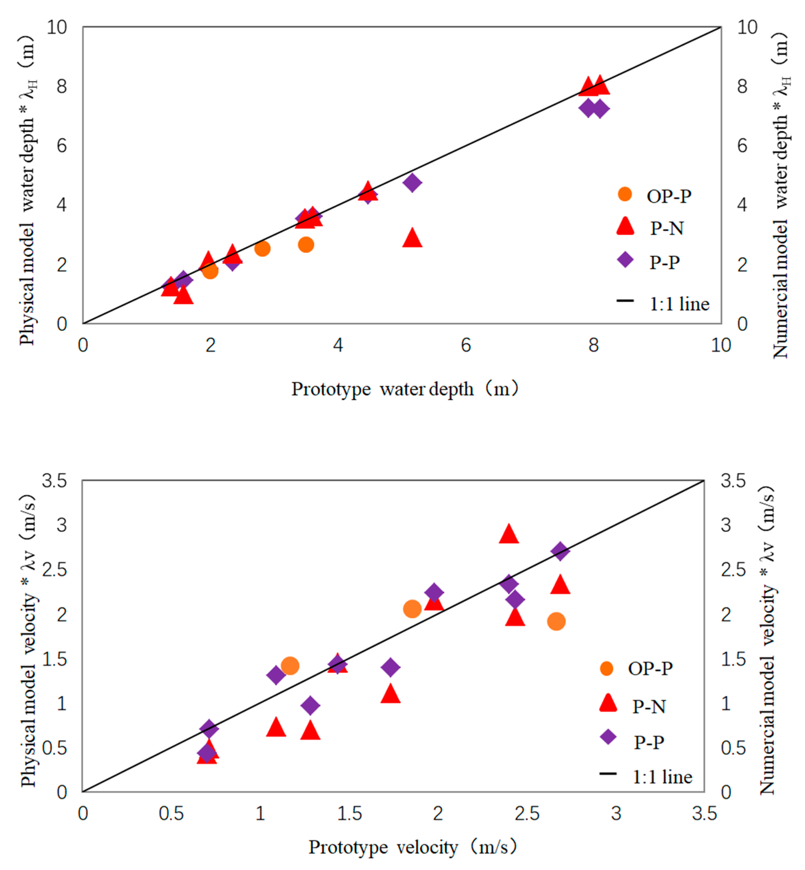
The MSPM and numerical model data are multiplied by the corresponding similarity scale during the comparison. The water depth from assimilation model is the averaged water depth at the discharge which equals to the bankfull discharge of the same cross-section. The velocity from assimilation model is also the average velocity of the cross-section which is computed as Q/A. Figure 4 shows that most of the water depth and velocity results are distributed near the 45-degree line (1:1 line). It can be inferred that the depth and velocity results derived from our MSPM is close to that of the assimilation model. The comparison between OP-P sequence and the P-P sequence presents that our MSPM can achieve similar experimental results with other physical models.
4. Discussion
4.1. Gravity Similarity Shift
Chen et al. [12] used a MSPM to carry out river model experiments and discussed the practicality of real-time water level, flow rate, and roughness coefficient updates by combining the particle filter-based assimilation model and the one-dimensional hydrodynamic model. Taking the average of the inverse calculated roughness coefficient in the above article, the actual roughness coefficient of the MSPM was 0.0536. This value differed from the given model roughness coefficient , which affected the model gravity and resistance similarity.
When = 0.015, = 0.0536, and m = 0.052, the velocity scale that satisfied the resistance similarity criterion was calculated as 8.987 by Equation (4). The value that satisfied the gravity similarity criterion was calculated as 7.071 by Equation (1). It can be seen that the model did not satisfy the gravity and resistance similarity requirements at the same time.
As the MSPM uses different scales in the transverse and longitudinal directions, it can be understood that the river channel was stretched horizontally along the centerline based on a horizontal scale of 1400, and the center line remained unchanged vertically. Although the deviation of model distortion to resistance and gravity was reduced by adjusting model ratio and roughness coefficients, the deviation extent still needed to be assessed. For river sections with a slow change in flow elements and less disturbance caused by buildings, the resistance similarity conditions could not be neglected, while the gravity similarity conditions deviated slightly. There is no consensus on the degree of deviation allowed; however, practical experience has indicated that in fluvial rivers when the inertial force and gravity similarity ratio are allowed to deviate, the deviation should not exceed 50% [8].
Continuous conditions of water flow:
Therefore, the discharge scale under resistance similarity conditions is and the discharge scale under gravity similarity deviation is .
Comparing the two discharge scales for the MSPM and prototype discharge scale , it was found that and were basically equal, indicating that the MSPM met the similar conditions of resistance, and gravity similarity had a deviation. The gravity similarity deviation degree is written as:
According to the above equation, it was concluded that the model gravity similarity deviation was within the allowable range.
Figure 5 shows a comparison of the discharge scale that met the similarity resistance and the measured discharge scale. Using analysis of variance, when F was less than the critical value F0.05 (1.34), there was no significant difference between the discharge scale that satisfied the similarity resistance and the measured discharge scale.
Based on variance analysis, it can be seen that the MSPM had a very good simulation effect. Although the gravity similarity had a slight deviation, it did not have a strong influence on the model discharge scale, and had a good applicability for predicting bankfull discharge change in the future. Therefore, it was possible to obtain a more accurate measured bankfull discharge scale in the MSPM by appropriately correcting the theoretical discharge scale:
where f is the fitting coefficient, and the closer the value is to 1, the better the micromodel prediction effect.
4.2. Analysis of Discharge Scale Segmentation
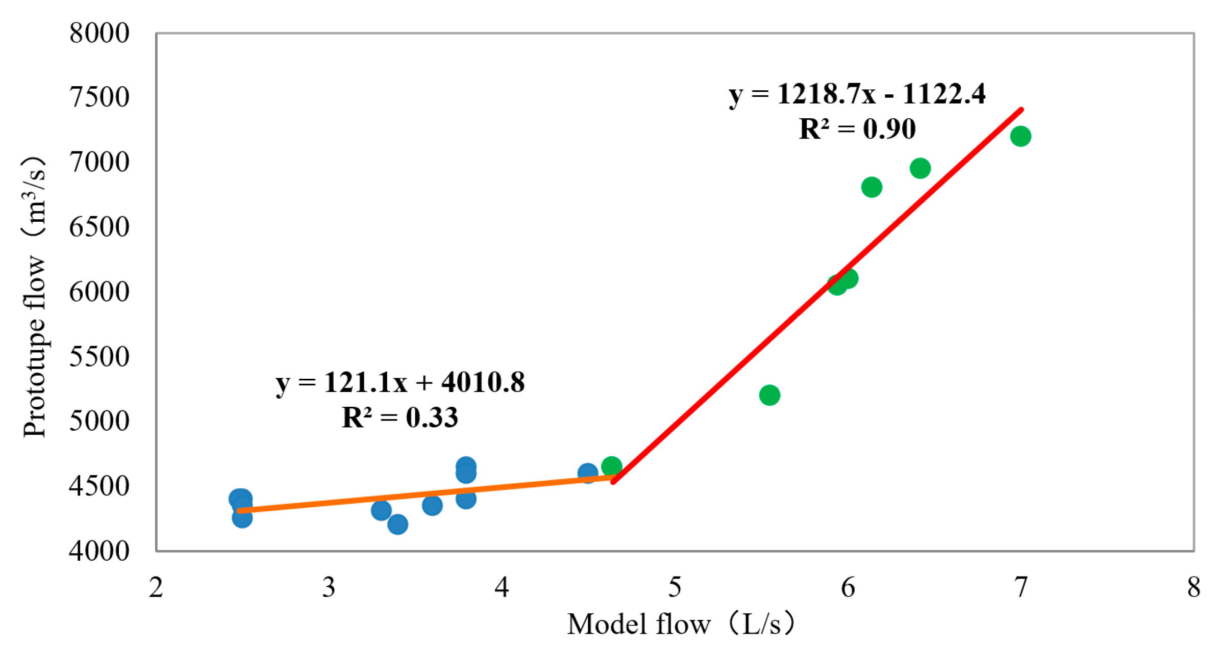
Further analysis was conducted on the relationship between the model and prototype bankfull discharge. A split-line rendering of the regression line may produce better results than the single line shown in Figure 3. When model flow was less than 4.5 L/s, the discharge scale was 121,100. When the model flow was greater than 4.5 L/s, the discharge scale was 1,218,700. Additionally, the discharge scale calculated according to the similarity criterion was between 121,100 and 1,218,700 (see Figure 6). The larger bankfull discharge group had a stronger linear correlation (larger R2).
After evaluating Figure 6, it can be seen that the large flow data was mostly concentrated in the river section near the upstream Xiaolangdi reservoir, and the discharge scale was relatively large. Small flow data was concentrated in the lower reaches of the GC, and the discharge scale was much smaller than upstream. Table 1 shows the main features of the two river reaches. The prototype roughness coefficients of the upstream reach DXY-GC and downstream reach GC-B3 were 0.01 [22] and 0.062 [16], respectively. The model roughness coefficients calculated from the numerical model data were the opposite for upstream and downstream. This may have been due to the non-wide and shallow cross-sectional shape and fixed boundary in the model.
The main reason for the two distinct flow ratios was presumed to be due to differences in slope adjustment and roughness design. The LYR has a wandering pattern in the reach from DXY to GC and the slope is relatively steep. The channel in the reach from GC to AS has a transitional pattern, and the reach from AS to B3 has a straight pattern with some sinuous segments [23]. The lower reach, from GC to B3, is a relatively stable meandering river reach with a gentle slope [24]. The slope of the upstream section of the model was adjusted more than downstream. Furthermore, flooding and sedimentation of the upstream riverbed during flood season is relatively large, and the mainstream swings frequently cause large changes in velocity. As velocity is a function of roughness coefficient, the rate of mean velocity with varying discharge reflects the roughness coefficient variability of channel boundaries [25]. Therefore, the changing river section roughness coefficient was more complicated. The reach from GC to B3 is a meandering section that is artificially controlled. The river section main stream does not shift horizontally, the velocity is relatively stable, and the influence on the roughness coefficient is small. In addition, adjustment of the transverse scale of microscale mode may also have influenced the discharge scale of the two river reaches.
4.3. The Effect of Three-Dimensional Distortion
Micromodels commonly use a distortion rate of 8 to 15 [1]. A large distortion rate raises concern about the ability of the model to reproduce flow conditions. However, there have been examples using a large distortion rate in hydraulic models. Ippen [26] incorporated distortions of up to 26.7 for an estuary model in 1968. Blench [27] utilized models with large vertical scale distortions. Our transverse distortion rate is close to 26.7, but our vertical distortion rate is larger. Therefore, we further analyzed the effect of the distortion rate on the simulated bankfull discharge.
Hydraulic slope scale is determined by the similarity of resistance in river model experiments and can be calculated by the equation [28]:
where is longitudinal distortion rate. The scale value is correlated with the vertical and longitudinal scales. The effect of large longitudinal distortion rate on slope scale is greatly reduced by m values that are much less than one.
The hydraulic radius of the cross-section is influenced by the transverse distortion rate. The scale of the hydraulic radius of the distortion model for a wide shallow channel is expressed as:
where are the river width and depth of the prototype, and the river width and depth of the model, respectively. is the transverse distortion rate. It can be seen that the scale of the hydraulic radius of the distortion model is related to both the transverse and vertical scales. When in a wide shallow channel, the effect of large transverse distortion on hydraulic radius scale is greatly reduced as well.
It is worth mentioning that the velocity scale in Equation (4) is a function of the slope scale and the hydraulic radius scale. Although it is affected by the large distortion rates in the longitudinal and transverse directions, it is acceptable for studying bankfull discharge, which has fewer requirements for flow field distribution, in terms of slope adjustment.
4.4. Application to Simulate Bankfull Discharge
In the LYR, bankfull discharge often refers to the flow at which water just fills a channel without overflowing the banks of the floodplain [29]. Since the 1950s, the geometric shape of cross-sections in the LYR reaches has changed significantly due to continuous channel adjustment. Cross-sectional profiles have been altered from their previous geometric shapes with high floodplains and low channels to high channels and low floodplains. Therefore, the bankfull discharge value is closely related to the cross-sectional profiles.
Due to the construction of a large number of water conservancy projects and the influence of human activities, the water and sediment conditions entering the LYR have changed significantly. This has also had a significant impact on the evolution of the channel. The river channel downstream of the reservoir has certain erosion over a long period of time, adjusting the shape of the river channel. The downstream river channel evolution usually includes continuous scouring of the river channel, section profile change, and flow capacity adjustments. From 1950 to 2003, the ratio of width to depth after the floodplain tended to increase slightly in LYR sections [10]. Cross-sections tended to be wide and shallow. The ratio of width to depth after the floodplain varied greatly in the HYK-SK reach and only slightly in the AS-LJ reach.
Profile changes in corresponding LYR sections can be expected according to the changing bankfull area data from previous years. The cross-section of the MSPM can then be adjusted based on the predicted profile. Discharge experiments will subsequently be repeated using the MSPM to obtain new bankfull discharge estimates. Bankfull discharge of the corresponding sections of the prototype can be calculated according to the fixed discharge scale. Such estimates can effectively diminish the flooding damage, and provide a technical reference for the following year’s water and sediment regulation in the LYR.
5. Conclusions
An indoor MSPM of the LYR was established and an automatic flow control system was used to carry out discharge experiments. Bankfull discharges of LYR sections were measured and compared with measured bankfull discharge in a river prototype. The results primarily illustrate that there was a relatively good correlation between model and prototype bankfull discharge. The correlation between the model and the prototype bankfull discharge was further validated according to the similarity theory and conditions of the MSPM.
The distorted scale model did not strictly satisfy the similarity requirements, but it still provided a solution to practical problems. In this paper, the slope adjustment method was used. By adjusting the riverbed slope to achieve resistance similarity, the adjustment coefficient m value that satisfied the similarity of gravity and turbulence resistance was determined to be 0.052. The results showed that although the gravity was similarly slightly deviated, it was within the allowable range. Large distortion rates in the longitudinal and transverse directions had limited influence on the velocity scale distortion, which was found to be acceptable for studying bankfull discharge. In the future, new bankfull discharge estimates for river cross-sections can be obtained by repeating discharge experiments as long as any new input data is obtained by trend analysis or numerical modeling.
Author Contributions
Conceptualization, M.C.; Methodology, X.Z. and M.C.; Software, F.X.; Tests: X.Z. and P.W.; Writing—Original Draft Preparation, X.Z.; Writing—Review and Editing, X.Z. and M.C.; Supervision, M.C.; Project Administration, M.C.; Funding Acquisition, M.C. All authors have read and agreed to the published version of the manuscript.
Funding
This research was made possible with the support of the National Key Research and Development Program (grant number 2016YFC0402506) and Chinese Universities Scientific Fund (grant number 2019TC157).
Acknowledgments
We are very grateful to Hongwei Fang of Tsinghua University for providing experiment sites, water and electricity facilities. We thank the editors and the anonymous reviewers for their constructive comments, which helped us to improve the paper. Acknowledgement for the data support from National Earth System Science Data Center, National Science and Technology Infrastructure of China. (htttp://www.geodata.cn)
Conflicts of Interest
The authors declare no conflict of interest.
References
- Maynord, S. Evaluation of the micromodel: An Extremely Small-scale movable bed model. J. Hydraul. Eng. 2006, 132, 343–353. [Google Scholar] [CrossRef]
- Gaines, R.; Smith, R. Micro-scale loose-bed physical models. In Proceedings of the Confernece on Hydraulic Measurements and Experimental Methods (CD-ROM), Estes Park, CO, USA, 28 July–1 August 2002; ASCE-EWRI & IAHR: Reston, VA, USA, 2002. [Google Scholar]
- Davinroy, R. River replication. Civ. Eng. 1999, 69, 61–63. [Google Scholar]
- Gaines, R.; Maynord, S. Micro-scale Loose-bed hydraulic models. J. Hydraul. Eng. 2001, 127, 335–338. [Google Scholar] [CrossRef]
- Davies, T.; McSaveney, M.; Clarkson, P. Anthropic aggradation of the Waiho River, Westland, New Zealand: Micro-scale modeling. Earth Surf. Process. Landf. 2003, 28, 209–218. [Google Scholar] [CrossRef]
- Echávez, G.; Ruiz, G. The use of mini—And micro-models to solve some type of problems. In Proceedings of the 2013 IAHR Congress, Chengdu, China, 8–13 September 2013. [Google Scholar]
- Maynord, S. Comparison of surface velocities in micro-scale model and prototype. In Proceedings of the Conference on Hydraulic Measurements and Experimental Methods (CD-ROM), Estes Park, CO, USA, 28 July–1 August 2002; ASCE-EWRI & IAHR: Reston, VA, USA, 2002. [Google Scholar]
- Li, W. Preliminary study on technology and theoretical basis of micro-scale model test. Port Waterw. Eng. 2012, 10, 69–73. (In Chinese) [Google Scholar]
- Mao, Y.; Huang, C.; Chen, J.; Zhou, J. Experimental study on the effect of sand mining and its control and utilization in Zhenjiang reach of the Yangtze River. J. Sediment Res. 2004, 3, 41–45. (In Chinese) [Google Scholar]
- Xia, J.; Wu, B.; Wang, G.; Wang, Y. Estimation of bankfull discharge in the Lower Yellow River using different approaches. Geomorphology 2010, 117, 66–77. [Google Scholar] [CrossRef]
- Xu, X.; Fang, H.; Lai, R.; Zhang, Y.; Huang, L.; Liu, X. A real-time probabilistic channel flood-forecasting model based on the Bayesian particle filter approach. Environ. Model. Softw. 2017, 88, 151–167. [Google Scholar] [CrossRef] [Green Version]
- Chen, M.; Pang, J.; Wu, P. Flood Routing Model with Particle Filter-Based Data Assimilation for Flash Flood Forecasting in the Micro-model of Lower Yellow River, China. Water 2018, 10, 1612. [Google Scholar] [CrossRef] [Green Version]
- Friedkin, J.F. A Laboratory Study of the Meandering of Alluvial Rivers; U.S. Waterways Experiment Station: Vicksburg, MS, USA, 1945; p. 40. [Google Scholar]
- Hu, C.; Cao, W. Variation, Regulation and control of flow and sediment in the Yellow River Estuary I: Mechanism of flow-sediment transport and evolution. J. Sediment Res. 2003, 5, 1–8. (In Chinese) [Google Scholar]
- Xia, J.; Wang, Z.; Wang, Y.; Yu, X. Comparison of morphodynamic models for the Lower Yellow River. J. Am. Water Resour. Assoc. 2013, 49, 114–131. [Google Scholar] [CrossRef]
- Hui, Y.; Wang, G. River Model Test; China Water & Power Press: Beijing, China, 1981. (In Chinese) [Google Scholar]
- Yellow River Institute of Hydraulic Research. The Consultation Report of Yellow River Institute of Hydraulic Research; Yellow River Institute of Hydraulic Research: Zhengzhou, China, 2008. [Google Scholar]
- Xia, J.; Wu, B.; Li, W. Comparison of different approaches to determine bankfull discharge in the Lower Yellow River. J. Sediment Res. 2009, 3, 20–29. (In Chinese) [Google Scholar]
- Ruan, X. Two-Dimensional Numerical Simulation Research on River Ice Dynamic Behavior of the Lower Yellow River. Ph.D. Thesis, University of Ocean, Qingdao, China, 2013. (In Chinese). [Google Scholar]
- Li, D.; Zhang, H.; Xu, Y.; Zhang, J. Finite simulation of 2-D flow in the Lower Yellow River. J. Sediment Res. 1999, 4, 61–65. (In Chinese) [Google Scholar]
- Dai, Q.; Hu, C.; Hu, J.; Chen, J. Experimental study on effects of flood peak discharge on formation of cross-section in the Lower Yellow River. J. Sediment Res. 2007, 3, 57–65. (In Chinese) [Google Scholar]
- Ma, Y.; Huang, H. Controls of the channel morphology and sediment concentration on flow resistance in a large sand-bed river: A case study of the Lower Yellow River. Geomorphology 2016, 264, 132–146. [Google Scholar] [CrossRef]
- Liu, X.; Shi, C.; Zhou, Y.; Gu, Z.; Li, H. Response of Erosion and Deposition of Channel Bed, Banks and Floodplains to Water and Sediment Changes in the Lower Yellow River, China. Water 2019, 11, 357. [Google Scholar] [CrossRef] [Green Version]
- Xia, J.; Li, J.; Zhang, S. Adjustment of riverbed in the lower Yellow River after the application of Xiaolangdi reservoir. Yellow River 2016, 10, 1000–1379. (In Chinese) [Google Scholar]
- López, R.; Barragán, J.; Colomer, M.Á. Flow resistance equations without explicit estimation of the resistance coefficient for coarse-grained rivers. J. Hydrol. 2007, 338, 113–121. [Google Scholar]
- Ippen, A. Hydraulic scale models. Osborne Reynolds Centenary, Osborne Reynolds and Engineering Science. Ph.D. Thesis, University of Manchester, Manchester, UK, 1968; pp. 199–224. [Google Scholar]
- Blench, T. Regime Behavior of Canals and Rivers; Butterworths Scientific Publications: London, UK, 1957. [Google Scholar]
- Wang, X. The feasibility analysis of three-dimensional metamorphic river model. J. Anhui Tech. Coll. Water Resour. Hydroelectr. Power 2002, 2, 6–9. (In Chinese) [Google Scholar]
- Wu, B.; Wang, G.; Xia, J.; Fu, X.; Zhang, Y. Response of bankfull discharge to discharge and sediment load in the Lower Yellow River. Geomorphology 2008, 100, 366–376. [Google Scholar] [CrossRef]
Figure 1.
The plane view of the indoor microscale physical model (MSPM) with controlling equipment.

Figure 2.
MSPM and prototype bankfull discharge variation map. The red line represents the change in the prototype bankfull discharge, and the blue line represents the change in the model bankfull discharge. SZ, DM, FZ, XHT, PL, DWZ, XMT, SG, and DTL represent the sections of Sunzhuang, Doumen, Fanzhuang, Xiaohetou, Penglou, Dawangzhuang, Xumatou, Suge, and Datianlou respectively.

Figure 3.
Relationship between the prototype and model bankfull discharge. The red line represents the regression line, and the gray shaded area represents the 95% confidence interval.
Figure 3.
Relationship between the prototype and model bankfull discharge. The red line represents the regression line, and the gray shaded area represents the 95% confidence interval.

Figure 4.
Comparison between prototype, physical model, and numerical model data (multiplied by the corresponding scale). OP-P represents the data from other physical model and prototype data sequence. P-N represents the assimilated numerical model and prototype data sequence. P-P represents the physical model and prototype data sequence.

Figure 5.
Comparison of the theoretical and measured discharge scale. The red line represents the measured model and prototype regression line, and the green line represents the model and prototype flow that met similarity criteria.
Figure 5.
Comparison of the theoretical and measured discharge scale. The red line represents the measured model and prototype regression line, and the green line represents the model and prototype flow that met similarity criteria.

Figure 6.
Scale segmentation diagram. The orange line represents the measured MSPM and prototype regression line near the estuary, and the red line represents the measured model and prototype regression line near the upper reaches.
Figure 6.
Scale segmentation diagram. The orange line represents the measured MSPM and prototype regression line near the estuary, and the red line represents the measured model and prototype regression line near the upper reaches.


Table 1.
Discharge scale of different river sections.
| Reach | Slope J | Roughness Coefficient n | λn | m | λv | λQ | |||
|---|---|---|---|---|---|---|---|---|---|
| Prototype | Model | Prototype | Model | λQ,M | λQ,R | ||||
| DXY-GC | 1/5025 | 1/150 | 0.010 | 0.077 | 0.130 | 0.0598 | 18.05 | 1,218,700 | 121,100 |
| GC-B3 | 1/9166 | 1/350 | 0.062 | 0.045 | 1.377 | 0.0468 | 1.92 | 1,263,500 | 134,400 |
© 2019 by the authors. Licensee MDPI, Basel, Switzerland. This article is an open access article distributed under the terms and conditions of the Creative Commons Attribution (CC BY) license (http://creativecommons.org/licenses/by/4.0/).
Share and Cite
MDPI and ACS Style
Zhang, X.; Chen, M.; Wu, P.; Xin, F. The Use of a Microscale Physical Model to Simulate Bankfull Discharge in the Lower Reaches of the Yellow River. Water 2020, 12, 13. https://doi.org/10.3390/w12010013
AMA Style
Zhang X, Chen M, Wu P, Xin F. The Use of a Microscale Physical Model to Simulate Bankfull Discharge in the Lower Reaches of the Yellow River. Water. 2020; 12(1):13. https://doi.org/10.3390/w12010013
Chicago/Turabian StyleZhang, Xue, Minghong Chen, Pengxiang Wu, and Fengmao Xin. 2020. "The Use of a Microscale Physical Model to Simulate Bankfull Discharge in the Lower Reaches of the Yellow River" Water 12, no. 1: 13. https://doi.org/10.3390/w12010013
Note that from the first issue of 2016, this journal uses article numbers instead of page numbers. See further details here.