Article

Assessing Suitability of Auto-Selection of Hot and Cold Anchor Pixels of the UAS-METRIC Model for Developing Crop Water Use Maps

1
Center for Precision and Automated Agricultural Systems, Irrigated Agriculture Research and Extension Center, Department of Biological Systems Engineering, Washington State University, Prosser, WA 99350, USA
2
Department of Biological Systems Engineering, Washington State University, Pullman, WA 99164, USA
*
Author to whom correspondence should be addressed.
Remote Sens. 2022, 14(18), 4454; https://doi.org/10.3390/rs14184454
Submission received: 30 June 2022 / Revised: 25 August 2022 / Accepted: 30 August 2022 / Published: 7 September 2022
(This article belongs to the Special Issue Remote Sensing-Based Evapotranspiration Models)

Abstract

:
The METRIC energy balance model uses an auto-selection approach for identifying hot (dry, bare soil) and cold (fully transpiring crop) anchor pixels for the internal calibration of the model. When an unmanned aerial system (UAS) is used for imagery, the small image size and the varying crop and soil water status of agricultural fields make the identification of reliable hot and cold pixels challenging. In this study, we used an experimental spearmint field under three irrigation levels (75%, 100%, and 125% of crop evapotranspiration, ETc). As a way of providing diverse field conditions, six different extents (Extent 1 to Extent 6) were selected from each day of the seven days of UAS imagery campaigns of the same field for generating UAS-based ETc maps using auto-selection of hot and cold anchor pixels for the internal calibration of the model. Extent 1 had the smallest coverage area of the field, including only plants that were irrigated at 75% of ETc, while the fields of view of the other extents increased to where the Extent 6 covered the spearmint field and all the surroundings including trees, a nearby water canal, irrigated grass, and irrigated and non-irrigated soil. The results showed that different sizes of extent resulted in the selection of variable hot (bare, but moist soil in small extents, and dry bare soil at the larger extents) and cold anchor pixels (crop under water stress at the small extents, and tree canopy or grass alongside the water canal at the larger extents). This variation resulted in significantly different ETc estimation for the same spearmint crop field, indicative of a potential limitation for the use auto-selection of hot and cold pixels when using the UAS-METRIC model.

1. Introduction

For site-specific and precision irrigation management, the use of high-resolution spatiotemporal models that can estimate crop water consumption throughout the season is important [1,2,3,4,5]. For this type of application, a small unmanned-aerial-system (UAS)-based energy balance model has been developed by implementing some modifications to the METRIC (mapping evapotranspiration at high resolution with internalized calibration) model in the “Water, R package” [6]. This model uses images from multispectral and thermal infrared cameras mounted on a UAS for estimating instantaneous crop evapotranspiration (ETc) as a residual of the surface energy balance [4,6,7]. Then, it uses weather-based daily alfalfa reference evapotranspiration to scale the instantaneously sensed ETc to daily ETc. The METRIC energy balance uses two anchor temperatures (hot and cold pixels) for internal calibration where the cold anchor represents the temperature of a fully irrigated crop, and the hot anchor is the temperature of dry bare soil with zero evapotranspiration (ET) [8,9]. The METRIC model uses these two selected extreme temperatures to calculate the surface temperature gradient between the land surface and air (dT) as described by Allen et al. [8]. The two pairs of dT and surface temperature (Ts) values for hot and cold anchors are used for determining “a” and “b” constants from the dT = aT s + b equation, where these constants are unique for each image. These parameters are used to calculate sensible heat flux (H) for the two extreme conditions and to conduct the internal calibration of the model.
A CIMEC approach (calibration using inverse modeling at extreme conditions) was defined by Allen et al. [10] for the auto-selection of hot and cold pixels in the Landsat METRIC model. In the CIMEC approach, the average temperature of 20% of the coolest pixels that also are in the top 5% of the normalized difference vegetation index (NDVI) is selected as the cold anchor temperature (Tcold), and the average 20% of the hottest pixels with the lowest 10% NDVI as the hot anchor temperature (Thot) [10]. In the current version of the UAS-METRIC model [4,7], there are some embedded range criteria for selecting hot and cold pixels such as the NDVI (cold: 0.76–0.84, hot: 0.10–0.28), albedo (cold: 0.18–0.25, hot: 0.13–0.15), leaf area index (LAI, cold: 3–6), and momentum roughness length (Zom, cold: 0.03–0.08, hot: ≤ 0.005) [6].
For the satellite-based METRIC model [8,9,10], hot and cold anchor pixels are found from satellite images that cover very large areas. Because UAS-based imagery covers a much smaller area, it might not be possible to find adequate cold and hot temperatures within the image of some fields. In this study, we used the auto-selection of hot and cold anchor pixels of the UAS-METRIC model to obtain the anchor temperatures from extents of UAS images of different sizes and assess their effect on ET estimations.

2. Materials and Methods

2.1. Study Sites

The study was conducted in a field of 0.55 ha located in Prosser, Washington, USA (46°15′4″N, 119°44′18″W) in the summer of 2021. This experimental field was located immediately next to a Prosser site AgWeatherNet (AWN) station. Prosser has a semi-arid climate with an average annual precipitation of 156 mm (based on historical data 2002–2022) with minimum rainfall in July and August.
The experimental field was planted to native spearmint. In 2021, this field was in the third year of growth. This field was irrigated by a linear move irrigation system (Valley 8000 Series model, Valley, NE, USA) moving north to south within the field. The linear machine has two spans, one of them using low elevation spray application (LESA) and the other one using mid-elevation spray application (MESA). The native spearmint was planted under the LESA span (Figure 1). The sprinklers in the LESA systems were 1.5 m apart from each other and 0.3 m from the ground level. The sprinklers had a Nelson D3030 body with the brown grooved fixed spray plate, a 41 kPa (6 PSI) pressure regulator.
A split-block design was used for this experiment. The field was divided into six blocks (replications), each consisting of three irrigation levels as the main variable and five nitrogen levels as the subplot variables. Varying nozzle sizes on the LESA system were used to control the different irrigation level treatments. The irrigation levels were a moderate deficit irrigation (75% of full crop evapotranspiration, ETc), full irrigation (100% ETc), and over-irrigation (125% ETc) as dictated by another companion experiment. The nozzle # 19 (5.79 L min−1 for pressure 41 kPa) (Nelson Irrigation Corporation, Walla Walla, WA, USA)—that was the original nozzle size designed for the LESA configuration for irrigating this field—was used for the over irrigation treatment. Nozzle sizes # 17 (4.61 L min−1) and # 15 (3.59 L min−1) were used for fully and deficit irrigation treatments. Each irrigation plot was irrigated with 6 nozzles (9 m wide). The corner irrigation plots had 7 nozzles 10.5 m long to irrigate the borders. The borders were not considered in the experiment. The irrigation treatment plots extended from north to south of the field in the direction of movement of the linear irrigation machine (Figure 1). Irrigation scheduling of the whole field was done based on weather-based estimation of daily evapotranspiration and soil moisture measurements by a neutron probe (explained in detail at Section 2.7) for the 100% irrigation treatment. At each irrigation event, the soil profile of the 100% irrigation treatment was filled up to field capacity.
The subplot variables of this experiment were different nitrogen treatments. The current recommendation of the nitrogen application for commercial spearmint growers in the Pacific Northwest was used with soil tests to determine the application rate for the 100% nitrogen levels [11]. There were 4 levels of ammonium sulfate (AMS or (NH4)2SO4) at 151 kg/ha (67% AMS), 225 kg/ha (100% AMS), 254 kg/ha (133% AMS), 376 kg/ha (167% AMS), and one level of Urea (CH4N2O) at 225 kg/ha (100% of the actual nitrogen). There were 3 replications of each fertilizer treatment, and each consisted of 8 rows of the crop in a 6 m × 60 m plot size (Figure 1). All the measurements were taken from different water stress levels of only the 100% AMS treatments for this research study.

2.2. Aerial Imaging Campaigns

For aerial imagery data acquisition, a small unmanned aerial system (sUAS, ATI AgBOT™, Aerial Technology International, Wilsonville, OR, USA) was used in this study with different onboard sensors including a long-wave thermal infrared imaging sensor with a 13 mm lens (11,000 ± 3000 nm; Duo Pro R, FLIR Systems, OR, USA), a multispectral imaging sensor (RedEdge 3, MicaSense, Inc., Seattle, WA, USA) with five bands (Blue, 475 ± 10 nm; Green, 560 ± 10 nm; Red, 668 ± 5 nm; Red Edge, 717 ± 5 nm; and Near Infrared, 840 ± 20 nm). Solar irradiance data were provided by an incident light sensor (DSL, MicaSense, Inc., Seattle, WA, USA) mounted on the UAS, facing skyward. Open-source ground control software (MissionPlanner, version 1.3.49, Ardupilot) was used to configure the multispectral imaging sensor to capture images at 85% and 80%, front and side overlaps, respectively. The flight altitude was set to 60 m above the ground level which provided multispectral images with a resolution of 4 cm pixel−1 and thermal infrared of 7 cm pixel−1. A 3DR Telemetry Radio (Version 2, Arduino, Somerville, MA, USA) was used for the connection between the ground station and sUAS. Twenty white alphabetic labeled rectangular cardboards (0.75 m × 0.50 m) and twenty aluminum pieces (0.12 m × 0.12 m) were used as ground sample points (GSP) to separate the different irrigation and nitrogen plots in the field. An image of a calibrated reflectance panel (CRP, MicaSense, Inc., Seattle, WA, USA) was captured with the multispectral camera at 1 m AGL before and after the UAS flight. The UAS imagery was taken in 7 days from 3 to 26 August of 2021. Then, the spearmint crop was harvested on 2 September 2021.

2.3. Aerial Imagery Preprocessing

A photogrammetry and mapping software (Pix4D Mapper, Pix4D, Inc., Lausanne, Switzerland) was used for image stitching to make a surface temperature orthomosaic (Thermal infrared) and for the five surface-reflectance orthomosaics (B, G, R, NIR, RE). The five-band image from the calibration reflectance panel was used for radiometric calibration of the multispectral orthomosaic. During the processing of the multispectral images, the Raster Digital Terrain Model (DTM) generated as a GeoTIFF. The DTM in this article is referred to as the digital elevation model (DEM). The Geographic Information System (QGIS) platform (ver.3.18.3, Open Source) was then used for georeferencing the thermal orthomosaic on the blue orthomosaic using the GSPs (whiteboards and aluminum pieces) that were located in the field before the UAS data acquisition. The thermal infrared orthomosaic was resampled to the resolution of the multispectral bands (3.9 cm pixel−1) using the “Nearest Neighborhood” method.
Then, six different sizes of shapefile layers were created in QGIS by cropping the primary multispectral images to different sizes or extents. These were named as Extents 1 to 6 which the coverage area of each Extent is described in Figure 2. Then, each Extent shapefile was used (by Clip Raster by mask layer) to extract the 5-surface reflectance layers and the thermal and DEM layers. So, for each day of UAS data acquisition, we had 6 datasets with different extent sizes and the UAS-METRIC model was run for each extent, separately. Overall, in this paper, we had used 42 datasets (7 UAS imagery campaigns and 6 extent sizes for each day).
Weather parameters within 24 h of UAS imagery at 15 min intervals were downloaded from the Prosser AgWeatherNet station (AgWeatherNet, Washington State University, WA, USA). A CSV file was created that contained the date and time stamp, solar radiation (Rs, W m2), wind speed (m s−1), relative humidity (RH %), air temperature (°C), and precipitation (mm). This file was used as an input to the model for estimating daily and hourly alfalfa-based reference evapotranspiration (ETr24, mm day−1 [9,12]).

2.4. UAS-METRIC

For all 42 datasets, the UAS-METRIC model was run using an “R package” (Water, [7]) following the steps and modifications described by Chandel et al. [4,7]. For the process of internal calibration, the “calcAnchors” function with the “flexible” method were used. The coordinates of the determined hot and cold pixels were used to visualize their locations within the thermal and generated ET maps with a (†) sign.

2.5. Thermal Canopy

Canopy temperature is an indicator of the water stress status. As the thermal raster image is one of the main components of the UAS-METRIC model, it was important to analyze the canopy temperature of crop under the different water stress levels separately. So, using the histogram of the NDVI raster, the threshold values 0.7 was selected to generate a vegetation mask by segmenting out the soil background from NDVI raster and setting the soil background to ‘not a number’ (NAN) [13,14,15]. Then, the binary vegetation mask was multiplied to the thermal map to obtain the canopy temperature only. This process was done for all 6 extents.

2.6. Feature Extraction

A shapefile layer with eighteen rectangular regions of interest (ROI) with equal dimensions of (4.5 m by 2 m) was created over the spearmint canopy around the area of the installed neutron probe access tubes at the three irrigation levels in the six blocks at 100% AMS treatments (Figure 1). Each ROI contained 5625 pixels. For each extent size, the mean and standard deviation of the ET of the pixels within the ROIs was extracted using the “Zonal Statistics” tool. The mean and standard deviation of the canopy temperature within each of these ROIs was extracted for each of the extents and for each day of data collection as well.

2.7. Soil Water Content

A calibrated neutron soil moisture probe (CPN 503 Elite HYDROPROBE ®, InstroTek ® Inc., Orlando, FL, USA) was used to monitor changes in soil volumetric water content (SWC). For the access tubes, 1.5-inch (38 mm) PVC pipe, pressure rated to 827 KPa (120 PSI), were installed in eighteen locations as shown in Figure 1 to the depth of 1.2 m. These neutron probe access tubes were installed between two spearmint plants. A rubber stopper size 10 was used to cover the access probes to prevent water entering the pipes. The depths of soil moisture measurements were 150, 300, 460, 610, 760, and 914 mm. Together these gave a measurement of the SWC to 990 mm. A sixteen second count duration was used for the measurements at each depth.
Additionally, two TEROS-10 (METER-Group Inc., Pullman, WA, USA) were installed in the 100% ETc and 100% AMS plots of block 3 at the depths of 60 mm and 150 mm to measure the soil’s volumetric water content (VWC) at the active root zone and below it. To convert the % VWC to depth of SWC, the value of the shallow sensor was multiplied by 595 mm (water content to the depth of the active spearmint roots) and the % VWC of the deepest sensor was multiplied by 395 mm (representing soil water content below root zone to the 990 mm measurements). Figure 3 shows the estimated SWC to 990 mm at different irrigation levels throughout the season as measured by the neutron probe and TEROS-10.

2.8. Stomatal Conductance of the Leaf

Stomatal conductance of spearmint leaves was measured using a leaf porometer, (SC-1, METER-Group Inc., Pullman, WA, USA) for observing the symptoms of water stress on the crop canopy under different irrigation levels. Measurements were made from 5 sun-exposed leaves from the spearmint canopy near the soil moisture probe access tubes. These measurements were made right after UAS imagery data acquisition.

2.9. Evapotranspiration Based on a Basal Crop Coefficient

The short-grass-based crop coefficients (Kc) of the mint crop at the three growth stages of initial (0.4), mid (1.1) and end-of-season (1.05) for arid and semi-arid climate were adjusted for the local weather conditions using wind speed, relative humidity, and crop height following the methods described in FAO-56 [16]. Then, the modified short-grass-based crop coefficients were converted to the alfalfa-based crop coefficient to calculate ETc as ET c ( FAO 56 ) = K c ( alfalfa based ) × ET r and this was compared with the ETc estimation from the UAS-METRIC model. This conversion was done since alfalfa-based reference evapotranspiration (ETr) is the main parameter used for scaling the instantaneous ETc to the daily ETc in the UAS-METRIC model.

2.10. Statistical Analysis

This study aimed to evaluate ET estimates of native spearmint at different irrigation levels using the UAS-METRIC model and with different sizes of extent. Once all the comparisons were done on the three irrigation levels (75% ETc, 100% ETc, and 125% ETc) of Block 1 only and in other analysis, ET estimation of all 18 plots were compared for each Extent sizes. Several one-way analyses of variance (ANOVA) were done in JMP ® software (version 8.0.8, SAS Institute Inc., Raleigh, North Carolina, USA) to compare the soil water content, ETc estimation of different extent sizes, canopy temperature, stomatal conductance of the native spearmint under different water treatment levels. A Tukey multiple comparison was used to define statistically significant differences (at 0.05 level) between the treatments.

3. Results

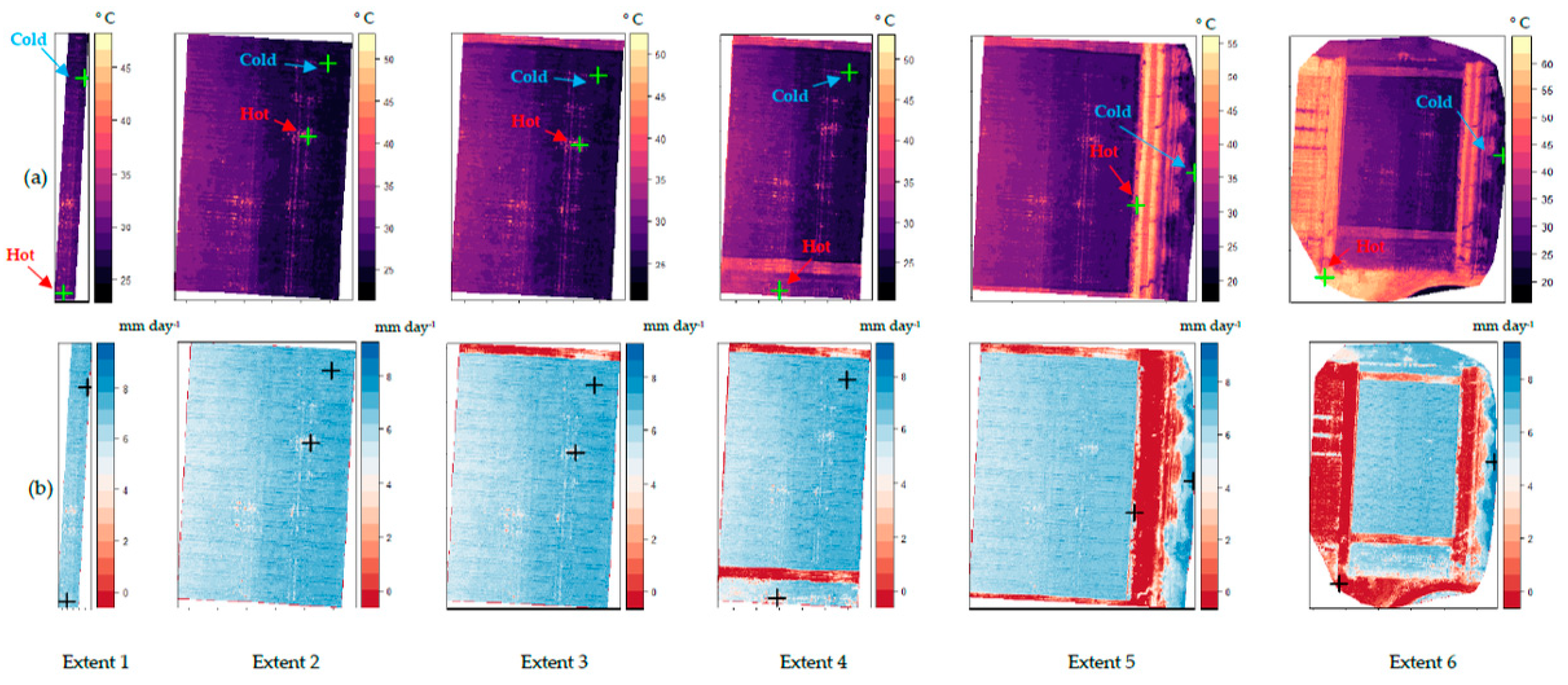
3.1. Hot and Cold Anchors

The characteristics of the auto-selected hot and cold anchor pixels from different extents of the UAS-METRIC model for two days 3 and 26 August are presented in Table 1. On 3 August, the crop canopy did not fully cover the ground. So, the UAS-METRIC model found a pixel of dry bare soil as the hot anchor pixel (Ts = 41.6 °C, LAI = 0.28, and NDVI = 0.33) at Extent 1. The details of auto-selected hot and cold pixels for all six extents of image shows that these pixels are selected from varying locations of the field with different LAI, and NDVI values (Table 1, Figure 4). The selected cold pixel in Extent 1 on 3 August, is a pixel of the spearmint canopy from the B1-75% of ETc irrigation treatment, while for Extent 2, 3, and 4 the selected cold pixel is from the crop canopy from the B2-125% ETc treatment (Figure 4). In Extent 5 and 6, the cold pixel was selected from canopy of the trees at the eastern side of field (Ts = 21.8 °C, LAI = 5.91, and NDVI = 0.84). For the generate map on 26 August (Table 1) and on 20 August, the cold pixel at the Extent 6 was selected from the green plant growing at the edge of the canal.
The selected hot pixels at Extents 1 to 4 of 3 August were from soil irrigated by the linear machine, while at Extents 5 and 6, the hot pixels were from the dry bare soil outside of the irrigated field (Figure 4). Among all extents, the hot anchored pixel at Extent 6 from dry bare soil outside the area irrigated by the linear machine was the hottest (Figure 4) selected anchors. Because of the differences in the selected hot and cold pixels for each Extent size, the calculated coefficient “a” and “b” varies for each extent and thus results in different ET estimations for each pixel (Table 1).
On 26 August, the crop was at the maturity growth stage, and it was fully covering the ground surface, so, the model was not able to detect a hot pixel within Extent 1, and the ET map was not generated (Table 1). At the different sizes of Extents 2 to 4, similar cold pixel from the spearmint canopy at B2-125% were selected (Ts = 22.13 °C, LAI = 5.42, and NDVI = 0.81).
Figure 5 shows temperatures of the auto-selected hot and cold anchor pixels for the different extent sizes, and for all seven days of data acquisition. The results show that the temperature of the hot pixels from Extents 5 and 6 that represents dry bare agricultural soils, are significantly higher compared to the temperature of the selected hot pixels from Extent 1 to 4 (Oneway ANOVA, 0.05 significant level). The selected hot pixel in Extents 1, 2, 3, and 4 were from the bare soil that was irrigated by the linear machine. Additionally, there were a slightly different (2 to 3 °C) in the temperature of cold pixels of different extent sizes (Figure 5). The selected cold pixel for Extent 2 to Extent 4 are from the crop canopy at the eastern side of the field (Block 2, 4, and 6) where the crop is cooler, possibly because of the shades of the trees, compared to the temperatures of spearmint canopy in the western half of the field (Blocks 1, 3, and 5). These results show that auto-selection of hot and cold pixel in UAS-METRIC model is unreliable method for the internal calibration of the METRIC model as it selects different anchor pixels based on the extent of the UAS flight mission or extent of image during image processing steps.

3.2. Daily ETc Estimation from Different Extents

The ETc maps generated by the UAS-METRIC model for all 6 image extents of all 7 days of UAS aerial imagery acquisition in August 2021 are shown in Figure 4. The ETc map for Extent 1 was only generated for 4 datasets (3, 5, 12 and 20 August) with pixels of the bare soil from the treatments. For the other 3 datasets, the crop canopy covered the soil surface, and the model could not generate the ETc map for the Extent 1 (Figure 6). This indicates that for a field with a fully covered ground surface without pixels of bare soil, the model will not be able to select a hot pixel for internal calibration and ETc estimation.
The mean ETc of the three defined ROIs at each irrigation level in Block 1 for all imaging campaigns with different extents are plotted in Figure 6. The results show that the ETc estimation extracted from the six extent sizes of the same spot in the field are different. The ETc estimation at Extent 1 and 2 was often very different compared to the other extents. Additionally, ETc for all three irrigation levels is estimated lower at Extent 2 where there was only crop canopy without clear exposure to bare soil. Extent 2 did not always fail to find hot pixels because the crop in some spots near the neutron probe access tubes was damaged by walking over the field during soil moisture data collection and these bare soil pixels were detected.
For the 20 August, ETc estimation by UAS-METRIC model for all irrigation levels was lower than the ETc of the other dates, which can be explained by cloudy conditions (Figure 6). For the last four days of UAS imagery data collection, the crop was fully covering the ground surface and the ETc of the native spearmint for the fully irrigated treatments should be closer to ETr. For all days in the study, the UAS-METRIC ETc value are significantly lower compared to the ETc (FAO-56) values. The underestimation of ETc by UAS-METRIC can be at least partially explained by the poor selection of hot and cold pixels from the auto-selection process of the UAS-METRIC model. Extent 2 significantly underestimated ETc on 5 and 24 August compared to other Extents (3, 4, 5, and 6) at all irrigation levels.

3.3. Canopy Temperature and Stomatal Conductance

The results showed no significant difference between the ETc estimation under different irrigation levels for all 7 days under the study (Figure 6). This was investigated and found to be due to no significant difference (Student’s t-test, at 0.05 significant level) between the canopy temperatures of the different irrigation levels of Block 1 which can be partially explained by the relatively low ETr rates on all seven days of data acquisition which would limit the separation between the irrigation level treatments (Figure 6). There was not enough water stress in the deficit irrigation crops to show differences even three to four days after irrigating the field (Figure 3). Additionally, the hourly mean air temperature of the installed ATMOS-41 in the middle of the field showed no statistically significant difference between the two temperatures (Figure 7).
Except for the 20 August that the stomatal conductance of the spearmint at the 125% ETc was significantly (Student’s t-test, at 0.05 significant level) higher compared to the other two irrigation levels, no difference was observed between the mean of the stomatal conductance for the other irrigation levels on the other days under the study.

4. Discussion

The results showed that all the hot pixels from the smaller extents (1,2,3, and 4) were selected from wet soils irrigated throughout the season. Based on the theory used to develop the METRIC model, hot pixels should be from dry bare agricultural soil where the latent heat of evaporation (LE) can be assumed to be nearly zero [8,9,10]. This situation would likely be common in practice for UAS-based images as most irrigated areas are large and dry bare soils may not be readily locatable within the imagery for a variety of reasons. In orchards or vineyards hot pixels might be automatically selected from shaded soil, which is cooler than dry, bare soil exposed to sunlight. For both scenarios, the auto-selection of hot pixels by the UAS-METRIC model can result in inaccurate ETc estimation. The availability of dry, bare soil within the limited field-of-view of UAS-based aerial imagery is not guaranteed in agricultural fields and orchards.
Additionally, the results showed that the same issue exists for selection of the cold anchor pixel within different sizes or extents. The cold pixel for the internal calibration of the UAS-METRIC model should represent a fully transpiring crop, not other things within the field of view of the UAS imagery like the nearby tree’s canopy or plants growing at the edge of the canal. Additionally, if UAS images are acquired from a large field with the whole field under water stress, an appropriate cold pixel is unlikely to be available within the limited field of view of the UAS-based imagery. In this study, Extent 1 simulates field condition with water stress crop and Extent 2, 3, and 4 represents spearmint canopy affected by shade of the trees and they were constantly cooler than crop canopy at the western side of the field (Blocks 1, 3, and 5) exposed to the sun. These were not appropriate cold pixels for the internal calibration of the model.
The variable selection of hot and cold anchor pixels within different extent sizes indicates the importance of providing a standardized hot and cold reference surfaces within the field-of-view of the UAS imagery that closely represent a dry and bare soil and a fully irrigated and fully transpiring crop canopy in the field. Using a calibrated reflectance panel is common for multispectral imagery to normalize the data because of the variation of sunlight after the UAS data acquisition [17]. Similarly, hot, and cold reference surfaces that can quickly stabilize their temperatures with the weather and environment can be used for the internal calibration of the model and can assist users to estimate ET accurately.

5. Conclusions

This research study found the following limitations for the UAS-METRIC model:
  • If the composite image is limited to a field with full crop cover and without visible pixels of a bare soil, the model cannot find hot anchor pixels, and it fails to generate a map of crop evapotranspiration.
  • The limits of the image size and the conditions of the crop and soil within the image affects the measured temperature of the hot and cold pixel reference conditions, and this results in different ET estimation outputs for the model. A field could be uniformly water-stressed or uniformly wet, for example, and a relevant fully irrigated cold pixel or hot (dry bare soil) pixel would not be available within the image.
The limited extents of imagery from the UAS-METRIC model cannot guarantee representative hot and cold pixel points at the required reference conditions. This points to the need to provide standardized hot and cold reference surfaces that, when placed within the UAS-based imagery, can quickly equilibrate with the ambient weather conditions and field microclimate to calibrate the UAS-METRIC model.

Author Contributions

Conceptualization, B.M., R.T.P., C.O.S. and L.R.K.; methodology, B.M., L.R.K., R.T.P. and C.O.S.; software, B.M., L.R.K., R.T.P. and C.O.S.; validation, B.M.; formal analysis, B.M.; investigation, B.M.; resources, L.R.K., R.T.P. and C.O.S.; data curation, B.M., R.T.P. and L.R.K.; writing—original draft preparation, B.M.; writing—review and editing, B.M., R.T.P., C.O.S. and L.R.K.; visualization, B.M., R.T.P., L.R.K. and C.O.S.; supervision, R.T.P., C.O.S. and L.R.K.; project administration, B.M., R.T.P., L.R.K. and C.O.S.; funding acquisition, R.T.P., L.R.K. and C.O.S. All authors have read and agreed to the published version of the manuscript.

Funding

This project was supported in part by the USDA National Institute of Food and Agriculture, projects 10164, WNP0839, Washington Mint Commission, Mint Industry Research Council (MIRC).

Acknowledgments

We would like to thank Abhilash K. Chandel for his assistance in the drone imagery data collection. Additionally, we thank Douglas B. Walsh as the principal investigator of the mint project, Ray Baker for his support for mint crop maintenance during the growing season, Russ Walsh for his assistance in neutron probe soil moisture data acquisition, John Paolo Sacdalan for assistance in stomatal conductance measurement.

Conflicts of Interest

The authors declare no conflict of interest.

References

  1. Mokhtari, A.; Ahmadi, A.; Daccache, A.; Drechsler, K. Actual Evapotranspiration from UAV Images: A Multi-Sensor Data Fusion Approach. Remote Sens. 2021, 13, 2315. [Google Scholar] [CrossRef]
  2. Zhang, H.; Yemoto, K. UAS-based remote sensing applications on the Northern Colorado Limited Irrigation Research Farm. Int. J. Precis. Agric. Aviat. 2019, 2, 1–10. [Google Scholar] [CrossRef]
  3. Barker, J.B.; Bhatti, S.; Heeren, D.M.; Neale, C.M.U.; Rudnick, D.R. Variable Rate Irrigation of Maize and Soybean in West-Central Nebraska Under Full and Deficit Irrigation. Front. Big Data 2019, 2. Available online: https://www.frontiersin.org/article/10.3389/fdata.2019.00034 (accessed on 13 January 2022).
  4. Chandel, A.; Khot, L.; Molaei, B.; Peters, R.; Stöckle, C.; Jacoby, P. High-Resolution Spatiotemporal Water Use Mapping of Surface and Direct-Root-Zone Drip-Irrigated Grapevines Using UAS-Based Thermal and Multispectral Remote Sensing. Remote Sens. 2021, 13, 954. [Google Scholar] [CrossRef]
  5. Chávez, J.L.; Torres-Rua, A.F.; Woldt, W.E.; Zhang, H.; Robertson, C.C.; Marek, G.W.; Wang, D.; Heeren, D.M.; Taghvaeian, S.; Neale, C.M. A Decade of Unmanned Aerial Systems in Irrigated Agriculture in the Western U.S. Appl. Eng. Agric. 2020, 36, 423–436. [Google Scholar] [CrossRef]
  6. Federico, G.O.; Ortega-Farías, S.; de la Fuente-Sáiz, D.; Fonseca, D.L.; Fuentes-Peñailillo, F. Water: Tools and Functions to Estimate Actual Evapotranspiration Using Land Surface Energy Balance Models in R. R J. 2016, 8, 352. [Google Scholar] [CrossRef]
  7. Chandel, A.K.; Molaei, B.; Khot, L.R.; Peters, R.T.; Stöckle, C.O. High Resolution Geospatial Evapotranspiration Mapping of Irrigated Field Crops Using Multispectral and Thermal Infrared Imagery with METRIC Energy Balance Model. Drones 2020, 4, 52. [Google Scholar] [CrossRef]
  8. Allen, R.G.; Tasumi, M.; Trezza, R. Satellite-Based Energy Balance for Mapping Evapotranspiration with Internalized Calibration (METRIC)—Model. J. Irrig. Drain. Eng. 2007, 133, 380–394. [Google Scholar] [CrossRef]
  9. Allen, R.G.; Tasumi, M.; Morse, A.; Trezza, R.; Wright, J.L.; Bastiaanssen, W.; Kramber, W.; Lorite, I.; Robison, C.W. Satellite-Based Energy Balance for Mapping Evapotranspiration with Internalized Calibration (METRIC)—Applications. J. Irrig. Drain. Eng. 2007, 133, 395–406. [Google Scholar] [CrossRef]
  10. Allen, R.G.; Burnett, B.; Kramber, W.; Huntington, J.; Kjaersgaard, J.; Kilic, A.; Kelly, C.; Trezza, R. Automated Calibration of the METRIC-Landsat Evapotranspiration Process. JAWRA J. Am. Water Resour. Assoc. 2013, 49, 563–576. [Google Scholar] [CrossRef]
  11. Mitchell, A.R.; Farris, N.A. Peppermint Response to Nitrogen Fertilizer in Central Oregon; Central Oregon Agricultural Research and Extension Center (COARC): Madras, OR, USA, 1994. [Google Scholar]
  12. Allen, R.G.; Walter, I.A.; Elliott, R.L.; Howell, T.A.; Itenfisu, D.; Jensen, M.E. The ASCE Standardized Reference Evapotranspiration Equation; American Society of Civil Engineers: Reston, VI, USA, 2005. [Google Scholar]
  13. Otsu, N. A threshold selection method from gray-level histograms. IEEE Trans. Syst. Man Cybern. 1979, 9, 62–66. [Google Scholar] [CrossRef] [Green Version]
  14. Lottes, P.; Khanna, R.; Pfeifer, J.; Siegwart, R.; Stachniss, C. UAV-based crop and weed classification for smart farming. In Proceedings of the 2017 IEEE International Conference on Robotics and Automation (ICRA), Singapore, 29 May–3 June 2017; pp. 3024–3031. [Google Scholar]
  15. Chakraborty, M.; Khot, L.R.; Peters, R.T. Assessing suitability of modified center pivot irrigation systems in corn production using low altitude aerial imaging techniques. Inf. Process. Agric. 2019, 7, 41–49. [Google Scholar] [CrossRef]
  16. Allen, R.G.; Pereira, L.S.; Raes, D.; Smith, M. Crop Evapotranspiration—Guidelines for Computing Crop Water Requirements—FAO Irrigation and Drainage Paper 56 Summary; FAO: Québec City, QC, Canada, 1998; p. 15.
  17. Use of Calibrated Reflectance Panels For MicaSense Data. MicaSense Knowledge Base. Available online: https://support.micasense.com/hc/en-us/articles/115000765514-Use-of-Calibrated-Reflectance-Panels-For-MicaSense-Data (accessed on 3 April 2022).
Figure 1. (a) True color image of the experimental field. (b) linear move irrigation system with LESA sprinkler configuration. (c) Locations of installed neutron probe access tubes, (d) Location of installed Teros 10 at two depths of 15 cm and 60 cm and ATMOS-41 which both were connected to the ZL6 data logger.
Remotesensing 14 04454 g001
Figure 2. Different extents (cropped areas) of the UAS imagery used by UAS-METRIC to generate ETc maps.
Remotesensing 14 04454 g002
Figure 3. Monitoring soil water content throughout the August 2021 by a neutron probe at three irrigation levels 75% ETc, 100% ETc, and 125% ETc and a continuous measurement of VWC by the TEROS10 sensors.
Remotesensing 14 04454 g003
Figure 4. (a) An example of location of auto-selected hot and cold anchor pixels by UAS-METRIC model from different extent sizes on the thermal image on 3 August 2021. (b) The generated ET maps by the UAS-METRIC model of the same day (3 August 2021) with similar extent sizes with indicating the location of selected anchors.
Remotesensing 14 04454 g004
Figure 5. Hot and cold anchor pixels from each image extent for the 7 data collection campaign days.
Remotesensing 14 04454 g005
Figure 6. Estimated ETc from generated UAS-METRIC maps with different Extent sizes at different irrigation levels (75% ETc, 100% ETc and 125% ETc of Block 1).
Remotesensing 14 04454 g006
Figure 7. (a) Canopy temperature at different irrigation levels of 75% ETc, 100% ETc and 125% ETc compared to the hourly mean air temperature measured by ATMOS-41. (b) Measured stomatal conductance of the crop under different irrigation levels in Block 1.
Remotesensing 14 04454 g007
Table 1. Summary details of selected hot and cold anchor pixels of the UAS-METRIC model in two days of August 2021.
ExtentsAnchors
(Pixel)
Ts (°C)Location of PixelsPixel LAIPixel NDVIab
3 August 2021Extent 1Hot41.6Soil within B5-75% ETc0.280.330.2987.68
Cold27.2Spearmint within B1-75% ETc5.330.81
Extent 2Hot41.5Soil within B4-75% ETc0.170.280.2469.80
Cold24.0Spearmint within B2-125% ETc5.340.81
Extent 3Hot40.2Soil within B4-75% ETc0.060.200.2572.61
Cold24.0Spearmint within B2-125% ETc5.340.81
Extent 4Hot43.3Soil at the 75% ETc near grass0.160.280.2263.23
Cold24.0Spearmint within B2-125% ETc5.340.81
Extent 5Hot51.1Non-irrigated soil outside the field0.160.280.1439.48
Cold20.8Canopy of trees at eastern side5.900.84
Extent 6Hot59.8Non-irrigated soil outside the field0.060.200.1027.38
Cold21.8Canopy of trees at eastern side5.910.84
26 August 2021Extent 1HotAutomatic Selection of hot anchors FAILED
Cold
Extent 2Hot28.73Soil within B4-75% ETc0.580.410.34−96.32
Cold22.13Spearmint within B2-125% ETc5.420.81
Extent 3Hot36.89Soil irrigated at the 125% rate0.100.240.13−34.63
Cold22.13Spearmint within B2-125% ETc5.420.81
Extent 4Hot37.13Soil irrigated at the 75% rate0.080.230.13−34.08
Cold22.13Spearmint within B2-125% ETc5.420.81
Extent 5Hot42.76Non-irrigated soil outside the field0.100.240.08−21.72
Cold22.11Trees canopy at eastern side5.300.81
Extent 6Hot43.93Non-irrigated soil outside the field0.080.220.07−16.79
Cold20.61Plants at the edge of the canal5.490.83
Publisher’s Note: MDPI stays neutral with regard to jurisdictional claims in published maps and institutional affiliations.

