Article

Distribution of Lanthanides, Yttrium, and Scandium in the Pilot-Scale Beneficiation of Fly Ashes Derived from Eastern Kentucky Coals

1
Center for Applied Energy Research, University of Kentucky, 2540 Research Park Drive, Lexington, KY 40511, USA
2
Department of Earth & Environmental Sciences, University of Kentucky, Lexington, KY 40506, USA
3
Department of Mining Engineering, University of Kentucky, Lexington, KY 40506, USA
4
Physical Sciences Inc., 20 New England Business Center, Andover, MA 01810, USA
5
Winner Water Services, 200 Clark St., Sharon, PA 16146, USA
*
Author to whom correspondence should be addressed.
Minerals 2020, 10(2), 105; https://doi.org/10.3390/min10020105
Submission received: 14 January 2020 / Revised: 23 January 2020 / Accepted: 24 January 2020 / Published: 26 January 2020

Abstract

:
In this study, Central Appalachian coal-derived fly ashes from two power plants were beneficiated in a pilot-scale facility in order to produce a product with a relatively consistent concentration of rare earth elements (REE). The <200-mesh final fly ash product was produced by removing the carbon- and Fe-rich particles prior to screening at 200 mesh (75 µm). The Plant D fly ash had high concentrations of CaO and SO3, which were diminished through the two months when the ash was being beneficiated, representing a consequence of the heat, humidity, and excessive rainfall in the Kentucky summer. The high CaO and SO3 concentrations through the early runs likely contributed to the lower REE in the <200-mesh products of those runs. Of the non-REE minor elements, Ba, V, Mn, Zn, and As showed the greatest between-run variations within the runs for each plant. The overall REE concentrations proved to be similar, both on a between-run basis for the individual fly ash sources and on a between-plant basis. Variations in fly ash quality will occur in larger-scale operations, so on-going attention to the fly ash quality and the response of the fly ash to beneficiation is necessary. Changes in the Plant D fly ash with time imply that both the freshness of the original ash and the length and conditions of its storage at the site of beneficiation could be factors in the quality and consistency of the processed fly ash.

1. Introduction

Rare earth elements (REE: collectively, lanthanides, Y, and Sc, after usage by Connelly et al. [1]) are crucial for the production of electronics, magnets, catalysts, metal alloys, optics, and other items needed in modern society [2,3,4,5,6,7]. The separation of REE from coal combustion products, particularly fly ash, holds potential as a viable source of this valuable class of elements [8]. As refractory, non-volatile elements, REEs are relatively enriched in fly ash owing to the combustion of most of the diluent coal [9,10]. Therefore, coal-combustion fly ash is considered to be a potential source of REE and other valuable elements [11,12]. In some studies, lanthanide has only been divided into light rare earth elements (LREE; La to Sm) and heavy rare earth elements (HREE; Eu to Lu), with Y sometimes included among the HREE [13]. Note that the division between LREE and HREE may vary between authors, so it is always prudent to closely examine individual explanations of the ratios. The LREE/HREE ratio [13,14] (HREE/LREE is used in some cases); LREY (La through Sm), MREY (Eu through Dy plus Y), and HREY (Ho through Lu); and critical (Nd, Eu, Tb, Dy, Y, and Er), uncritical (La, Pr, Sm, and Gd), and excessive (Ce, Ho, Tm, Yb, and Lu) groups [12,15], are other criteria used to evaluate the commercial potential of elements. For critical, uncritical, and excessive groups, the divisions are somewhat subjective and are dependent upon current needs and reserves.
The major minerals in coal generally undergo transformations on the path to the molten phase and on the cooling path to fly ash. Clays melt and then form an amorphous glass; quartz undergoes phase transformation to the high-T form, β-cristobalite (cristobalite can also crystallize from the Al-Si-rich melt), and pyrite oxidizes, with the Fe ending up in Fe-oxides [16,17,18,19].
The association of REE in fly ash has been debated. While large (10′s of microns) REE-phosphates (including monazite), REE-carbonates, and zircons have been observed in coal, most of the minerals in coal-derived fly ash are much finer and, in general, the optical microscope-observable minerals cannot fully account for the REE concentrations in many fly ashes. The melting temperatures of monazite and zircon are well above boiler temperatures (>1400 °C), so melting would not seem likely. Monazite, at least, will shatter at boiler temperatures, perhaps due to expansion of the He trapped in the crustal lattice following its production from the radioactive decay of Th, one of the common elements in monazite [20]. The fine monazite and other minerals are entrained in glass in the fly ash [20,21,22,23]. REEs are also associated with nano-scale carbons surrounding the fly ash glass and spinels [20,24].
In Phase I of this study [21], several ashes (four pulverized coal combustion (PCC) ashes and one fluidized bed combustion (FBC) ash) were beneficiated on a bench-scale array involving froth flotation of the carbons, magnetic separation of the Fe-spinels (magnetite), and screening to produce a <200-mesh (<75-µm) Al-Si-rich ash product. Additional testing was conducted on the ponded ash from one of the PCC plants, which was a retired 1950′s-vintage, four-unit plant. In that case, a composite sample from 20 individual sampling points was subjected to a more thorough analysis (particle sizing, elemental analysis, chemical and mineralogical composition, optical petrography, x-ray diffraction (XRD), and high-resolution transmission electron microscopy (HRTEM)) than was done for the other ashes. The ponded ash was being excavated and relocated at the time of our sampling, with the new location being a landfill on another property of the same company.
For the current study, the original plan was to use that same ponded ash (albeit from the landfill). Following a consideration of the logistics in recovering ash from a covered landfill, it was determined that the ash would be acquired from a stockpile of never-ponded ash at the retired power plant (see Section 2. Methods) and from the fly ash produced by a 100-MW unit at another power plant. In the end, the two ashes were beneficiated in order to produce 12-13 tons of ash for the pilot-scale chemical processing.

2. Materials and Methods

Fly ash was obtained from Plants D (ca. 6 tons) and I (ca. 12 tons) (letters assigned from earlier CAER studies [25,26]) in June 2018 and August 2018, respectively. The second ash was acquired when the supply of first ash was exhausted; they were not co-mingled in processing. In both cases, the fly ash was the product of the combustion of Pennsylvanian-age eastern Kentucky coal; in general, the coal coming from a number of mines in Perry and Clay counties (based on communications with Hower by utility personnel).
The ashes were stored outdoors at the Center for Applied Energy Research facility (north of Lexington, Kentucky) on a tarp, surrounded by a silt fence, and covered when not in use (Figure 1). Lexington experienced its wettest year on record in 2018, receiving 183 cm of rain compared to an average of 117 cm, with early 2019 also having above-normal precipitation, so, despite efforts to keep the ash dry, the feed ash was at least damp at the beginning of the process.
Based on the information gathered in the Phase I investigation [21] and from test samples of the ashes processed here (Table 1 shows examples of the raw data), a beneficiation flowsheet was designed to optimize the production of a fine (<200 mesh; <75 µm) Al-Si fly ash with a minimum of carbon and magnetics. For the processing, the ash was transferred from the pile to a feed bin, with a conveyor leading to a 500-gallon (1893-L) agitated slurry tank (the general scheme is shown in Figure 2). About 400 lbs. (181 kg) of ash was used for each run. The slurry was screened at 16 mesh (1 mm) in order to remove any coarse particles. The underflow from the screen was passed to the froth flotation cells. The froth flotation circuit consisted of two agitated flotation cells (30 L each) arranged in series with an adjustable weir at the discharge of each cell, such that the retention time for the circuit could be controlled by adjusting each weir. A fuel-oil-based collector was added to selectively adsorb onto carbon particles to induce hydrophobicity. The dosage of collector depended on the amount of carbon present (the C was determined in the analysis of a test fraction of the bulk sample). Air bubbles were generated by air drawn through the hollow shaft of each agitator, with glycol frothing agent added to facilitate bubble generation, such that a sufficient bubble surface area could be generated for the attachment of hydrophobic carbon particles. Once bubbles transported carbon particles to the cell surface, a stable froth was formed and removed by mechanical scrapers. Flotation tailings then flowed across a drum magnetic separator (for the Plant I ash) to collect spherical magnetic particles. The remaining low-C, low-magnetics slurry was then separated into coarse (+200 mesh or +75 μm) and fine (−200 mesh or −75 μm) particles using a vibratory screen. The −200 mesh slurry was pumped to tanks which served as thickeners, whereby particles settled and clarified water was decanted. Clarified water from thickening was recirculated to the feed tank and make-up water was added to maintain the desired slurry pulp density. Once the desired amount of feed was processed (typically 300 to 400 kg), the thickened solids (typically 60–70% solids) were transferred to shallow bins and allowed to air dry to produce the final fine product (~20% moisture) and stockpiled for use as feedstock for chemical processing for REE recovery.
Splits of the dried product and of selected intermediate streams (carbons, magnetics, <200-mesh ash, etc.) were retained. The samples of the individual <200-mesh products were submitted for chemical analyses. The bulk of the <200-mesh product was placed in one-ton bags (Figure 3) and ultimately shipped to Winner Water Services (Sharon, PA) for the chemical extraction of REE from the processed ash (not described further here). The two ashes were not co-mingled in processing and the one-ton bags each contained the processed ash from just one of the sources.
Moisture, ash, and carbon analyses (the latter from the ultimate analysis) were conducted at the University of Kentucky Center for Applied Energy Research (CAER), following the appropriate ASTM standards. Major oxide and minor element concentrations (V through Pb in Table 2 and in supplementary Table S1) were quantified on a Rigaku ZSX Primus IV X-ray fluorescence unit at the CAER.
Particle size analysis was conducted on a Cilas 1090 Laser Particle Size Analyzer (France) at the CAER using the liquid-dispersion mode. The instrument has a measurement range of 0.04–500 μm.
The REE + Y + Sc (REYSc) were extracted from the fly ash samples by heated digestion with a 1:1 HF:HNO3 acid mixture, followed by analysis by inductively coupled plasma atomic emission spectroscopy (ICP-OES) at the CAER.
The use of ICP-AES (also known as ICP-OES for optical emission spectroscopy) versus ICP-MS (inductively coupled plasma mass spectroscopy) has been discussed by Ardini et al. [27] and Medvedev et al. [28], among others, with generally favorable results. For this study, a digested fly ash sample from each of the power plants was analyzed by ICP-OES by Physical Sciences Inc. personnel using an Agilent 5110 instrument. ICP-MS of the exact same samples was performed as a contract service by the University of Massachusetts Lowell Core Research Facility, using an Agilent 7900 ICP-MS. Both instruments were calibrated externally using standard solutions purchased from Sigma Aldrich. For some elements (La, Ce, Sm, and Y in Plant D; Sm and Pr in Plant I), ICP-MS produces higher numbers than ICP-OES. In general, the comparisons between the two methods were favorable, although we note that neither the odd-number heavy REE nor Yb are reported in this comparison (Figure 4).

3. Results

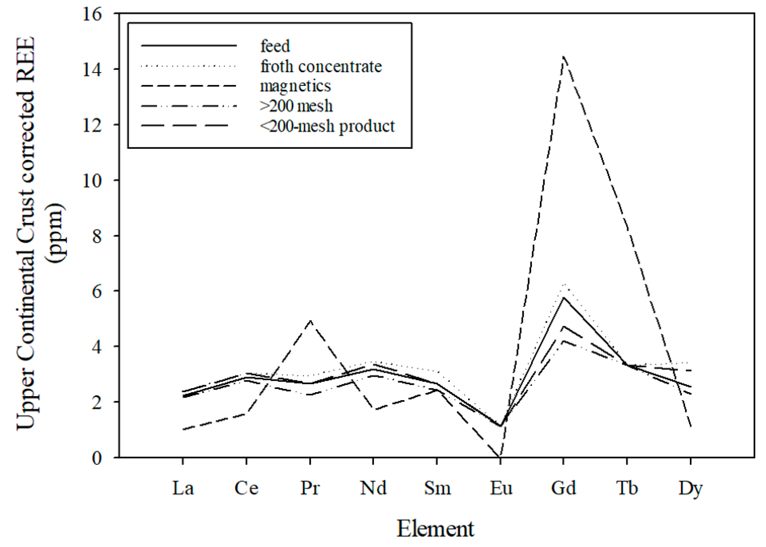
3.1. Multiple Fly Ash Products

The two feed samples differ not only in the power plant location, but in their source within the plant. The Plant D ash was in an area above the boiler, while the Plant I ash was from a bunker intermediate between the electrostatic precipitator hoppers and the ash landfill. The Plant D feed ash was notably coarser, with more of the ash being rejected by the 1-mm screen ahead of the beneficiation. The relative coarseness is no longer observable in the particle size distribution of the product ash, with the processed Plant I ash being coarser than the Plant D ash (Figure 5). With a consideration of the yield, loss-on-ignition (LOI), REE (concentration in ppm), and REE recovery (% of the feed ash REE content) for one run from the processing of ash from individual plants, the Plant D recovery is greater than the Plant I recovery owing to the lower amount of carbon and magnetics in the feed ash (Table 1).
As an example of the detailed chemistry of the fly ash fractions, the results from run 42 (Plant I) are shown in Table 2. Some trends are expected: the highest Fe is in the magnetic fraction, the highest C is in the froth flotation concentrate, and the highest Si and Al are in the <200- and >200-mesh fractions. By design, the highest REE (REYSc in the table) is in the <200-mesh fraction. Less anticipated is the high Pr, Gd, and Tb in the magnetics fraction, also the lowest REE concentrate. The Gd concentration in the magnetic fraction is 17.30% of the total lanthanides compared to an average of 5.17% in the Plant I <200-mesh product samples. The Pr, Gd, and Tb enrichment is even more apparent in the spider plot of the Upper Continental Crust-corrected REE concentrations (Figure 6 for La through Dy; correction factors after McLennan and Taylor [29]); the magnetic fraction stands out in having a notably different pattern than the other fractions. The high Gd, in particular, was observed in other magnetic fractions in this study and in the Phase I screening (Hower et al. [21]; the Gd enrichment in the magnetic fraction was not specifically mentioned in that paper, but the data is shown in their Table 8).

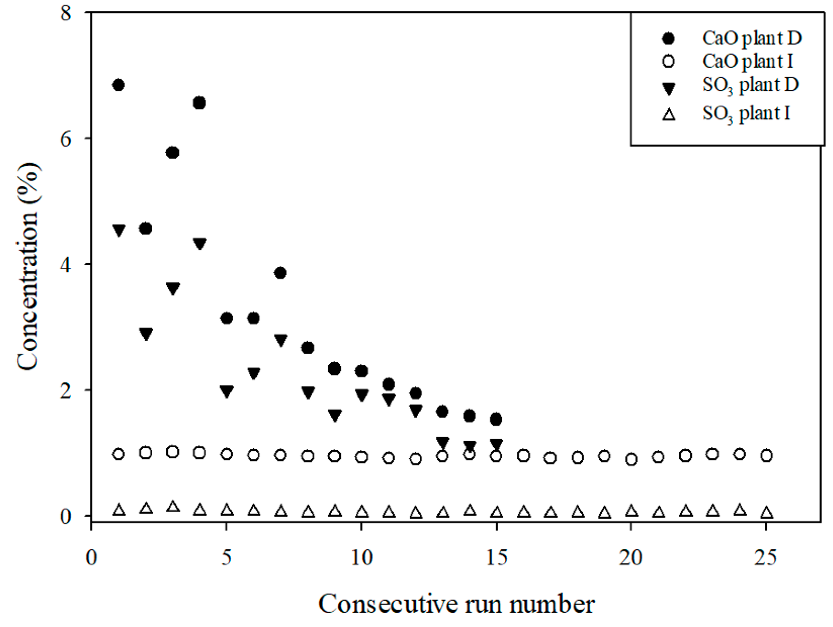
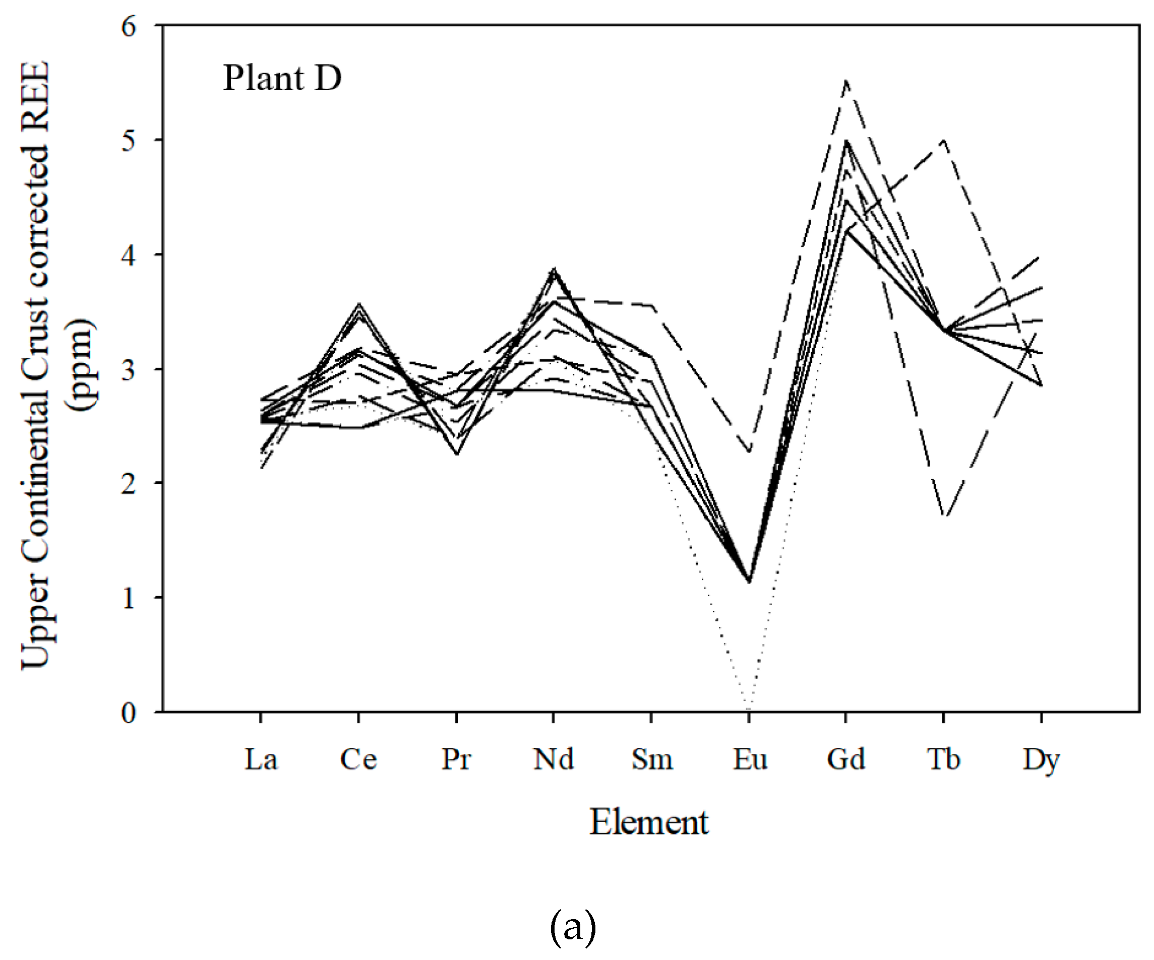
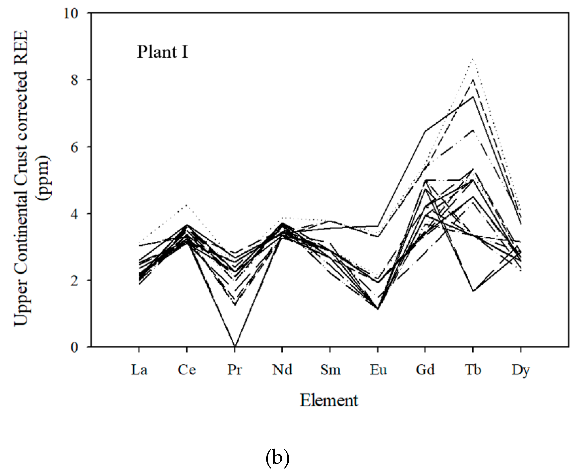
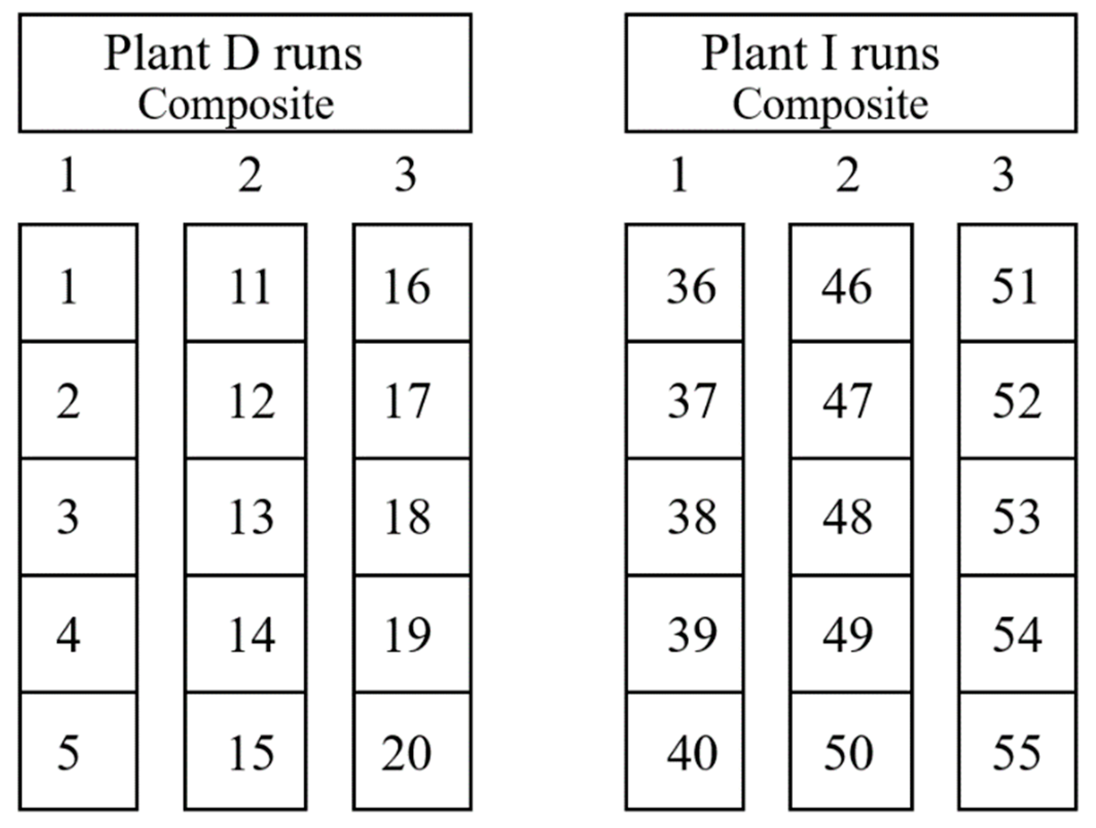
3.2. Individual Runs

The chemical analyses of the final, <200-mesh product from 15 runs of the Plant D fly ash and 25 runs of the Plant I fly ash, each representing about 180 kg of raw fly ash, are shown in Table S1. Consecutive run numbers imply that the runs were close in time, and sometimes on the same day.
The most obvious difference between the two plants is the abundance of CaO and SO3 (as gypsum) in the Plant D fly ash (Figure 7; Table S1). The Plant D ash was retrieved from a bunker above the boiler, so it had been exposed to a prolonged warm environment. It was inside the plant, protected from rain, but not from humidity. The source of the CaO and SO3 would have been from the gases associated with coal combustion, although the coal sources are not known as being enriched in CaO and the coals typically burned at both plants fall in the 1–2% S range. The loss of gypsum, contributing to the decline in the CaO and SO3 over the two months of processing, can be attributed to the heat, humidity, and, in particular, excessive rainfall of the Kentucky summer. While every attempt was made to keep the ash pile covered, exposure of the ash when the run’s ash supply was being transferred from the pile to the tank was unavoidable. The combination of humidity and rain served to leach CaO and SO3 from the ash. In contrast, the Plant I fly ash shows little variation in CaO and SO3. Overall, the CaO and SO3, and to a lesser extent, the C, dilute the concentration of REYSc in the product.
Among the non-REE minor elements analyzed (Table S1), within each plant, all of the elements show little between-run variation. Only Ba, V, Mn, Zn, and As show >1.3-times variation between the average compositions within each plant.
The REE are quite similar, both between the runs and between the averages for the two plants (Table S1). The highest-concentration elements (Sc, Y, La, Ce, and Nd), in particular, show remarkable similarity, in spite of the different concentrations and behavior of CaO and SO3 between the plants. The spider plots of the Upper Continental Crust-corrected REE concentrations of all the individual runs from Plants D and I are shown in Figure 8a,b, respectively. The variation in some elements is driven by low or non-detectable concentrations (Eu; plus non-detectable Pr concentrations, unusual for an element generally in the 9–21-ppm range). As with Figure 6, Ho through Lu were not plotted due to uncertainty in the odd-number REEs. The apparent extreme swings in the Tb concentration, particularly for Plant I (Figure 8b), are a reflection of an uncorrected range of 1–5 ppm, implying low concentrations with a relatively high variation.

3.3. Analysis of Variance

An analysis of variance (AOV) experimental design (Figure 9) was followed for the statistical evaluation of five parameters (Table 3). The AOV was a one-way/two-level design, with the levels being the two plants; then, by three sets of five consecutive runs (for this purpose, each set is considered to be a composite of those five runs); and followed by five individual runs in each “composite”, treated as replicates of the composite samples. Some of the significant variations (Table 4) in the plant and composite levels for CaO and SO3 and the plant level for carbon are obvious from an examination of Table 3 and Table 4. The composite-level variation in the REE is more subtle. While the plant averages (for the 15 samples per plant in the AOV analysis) are similar, with values of 530 vs. 515 ppm, the five-run composites vary much more; up to 480 ppm for one Plant D composite, to over 550 ppm for the other two composites in that group.

4. Discussion

Overall, the variation in REE seen in the variation between the individual runs (Table 2) smooths out at larger scales; the REE averages for the two plants are virtually the same (510 vs. 514 ppm), with similar standard deviations (45 vs. 43 ppm, respectively) (Table 2 plant averages). Certainly, some of the similarity between the plants was fortuitous, if not planned, as our selection of plants was driven by the knowledge that Central Appalachian-derived coals have higher REE contents than other sources, such as Illinois Basin-derived ash, available in Kentucky power plants.
Full-scale beneficiation and subsequent chemical processing would operate at a larger scale than seen with the individual runs. This does not discount variation in the overall ash supply with time. The coal supply changes over time, sometimes subtly and sometimes more dramatically. Beneficiation smooths out some of the variation, just as it did in this investigation, but it cannot economically create a high-REE feed out of an ash with a low REE concentration and it would be limited if the raw ash had greater percentages of rejects (meaning >1-mm feed ash, carbon, and magnetics, and >200-mesh post-flotation/post-magnetic separation ash). Therefore, the design of the total process would be an on-going procedure, with subsequent impacts on the beneficiation output and on the rate of production of REE concentrates.
The variation in other parameters between the plants and over time within a single ash source is greater, as demonstrated by the CaO and SO3 variation within the Plant D runs and between Plant D and Plant I. If such major oxides prove to impact chemical processing, the variation will need to be further smoothed out, if not eliminated entirely, by avoiding the problem supplier. The between-plant variation in carbon is another factor in processing; the variations among coal sources, grinder designs, and boiler configurations all contribute to varying amounts, sizes, and properties of fly ash carbon. Despite the flotation step in beneficiation, not all of the carbon can be efficiently diverted from the <200-mesh product.
The freshness and storage conditions of the ash can impact its overall quality, not just the REE content of the product. As seen in the chemistry of ashes, the CaO and SO3 of the Plant D ash changed over the course of the short time (less than 2 months) that it was being processed (Figure 7; Table 2). The original ash quality was a function of the storage of this ash at the plant and the change over time was likely a function of the weathering of the ash at the CAER. Only at the end of the supply of this fly ash did it approach a relatively constant composition of Plant I fly ash product. The high CaO and SO3 due to the addition of minerals not related directly to the production of fly ash and the consequent dilution of elements in the remainder of the ash may have been a factor in the lowered REE among the products from the first five runs of the Plant D ash versus the products from runs 11 to 20, presenting an average of 480 versus 554 ppm (Table 3).

5. Conclusions

Fly ashes from two power plants, both burning blends of Central Appalachian coals, were beneficiated in order to produce a product with a relatively consistent concentration of REE. The feed for the process was screened to eliminate +1-mm particles and the ashes were further processed to remove the carbon- and Fe-rich particles prior to screening at 200 mesh, with the <200-mesh fly ash being the final product. Each pilot-scale run processed about 180 kg of fly ash. While the beneficiation designs were specific to the fly ashes procured for this study, in large-scale processing, the ash quality may vary through the life of the operation. Just as in coal or mineral processing, the beneficiation design would be subject to change as the ash quality changes.
Plant D, with fly ash stored within the then-retired plant, had high concentrations of CaO and SO3. The original concentration, at least of the SO3, may have been from exposure to flue gas. The CaO and SO3 concentrations diminished through the two months when the ash was being beneficiated, which was a consequence of the heat, humidity, and excessive rainfall in the Kentucky summer. The ash pile was covered and, hence, somewhat protected from the rain, but some exposure was unavoidable. The high CaO and SO3 concentrations through the early runs likely contributed to the lower REE in the products of the same runs. The original Plant D ash quality and its change through storage implies that both the freshness of the original ash and the length and conditions of its storage at the site of beneficiation could be factors in the quality and consistency of processed fly ash. In contrast to Plant D, Plant I showed little variation in CaO and SO3.
Of the non-REE minor elements, Ba, V, Mn, Zn, and As showed the greatest between-run variations within the runs for each plant. The REE concentrations were similar, both between the runs for each fly ash source and in the average REE concentrations of the two sources.
While the overall goal in fly ash processing is to produce, as best as possible, a uniform feedstock for downstream processing, no two fly ashes will behave exactly the same in beneficiation. Each beneficiation flowsheet is designed for the specific ash and unit operations can be added or deleted, depending on the nature of the ash. The general principles of ash beneficiation outlined here will translate into the processing of other ashes, at least to other Appalachian-coal-derived and similar fly ashes, but the exact scheme must be individually designed based on a consideration of the properties of each ash.

Supplementary Materials

The following are available online at https://www.mdpi.com/2075-163X/10/2/105/s1: Table S1: Chemistry of individual runs from Plant D and Plant I.

Author Contributions

J.C.H. and J.G.G. directed the project at the CAER; J.C.H. oversaw the sampling and analytical aspects of the CAER project; J.G.G. designed the processing flow sheet for each fly ash; J.G.G., J.D.W., and D.T.M. processed the 18 tons of fly ash; S.D.H. and T.D.M. were responsible for the analyses of the samples at the CAER; P.J. was the PI of the overall project; P.J., D.V.P., and D.P.G. organized the PSI end of the project, including the comparison of analytical techniques discussed in the Methods; T.B. and M.S. were responsible for the Winner Water Services end of the project and, as the recipients of processed ash, they were part of an ongoing discussion with CAER and PSI concerning aspects of the pilot-scale beneficiation; J.C.H., J.G.G., and D.P.G. wrote the original draft of the paper; and everyone participated in the review and editing of the final submitted manuscript. All authors have read and agreed to the published version of the manuscript.

Funding

This study was completed as part of the U.S. Department of Energy contract DE-FE0027167. We thank our editors and reviewers for their constructive remarks.

Acknowledgments

We thank the personnel at the utility for their assistance in identifying and retrieving fly ash supplies for our investigation.

Conflicts of Interest

The authors declare no conflicts of interest.

References

  1. Connelly, N.G.; Hartshorn, R.M.; Damhus, T.; Hutton, A.T. Nomenclature of Inorganic Chemistry: IUPAC Recommendations 2005; Royal Society of Chemistry: London, UK, 2005. [Google Scholar]
  2. Greene, J. Digging for rare earths: The mine where iPhones are born. 2012. Available online: http://www.cnet.com/news/digging-for-rare-earths-the-mines-where-iphones-are-born/ (accessed on 25 January 2020).
  3. Hatch, G.P. Dynamics in the Global Market for Rare Earths. Elements 2012, 8, 341–346. [Google Scholar] [CrossRef]
  4. Dobransky, S. Rare Earth Elements and U.S. Foreign Policy: The Critical Ascension of REEs in Global Politics and U.S. National Security. American Diplomacy. 2013. Available online: http://www.unc.edu/depts/diplomat/item/2013/0912/ca/dobransky_rareearth.html (accessed on 25 January 2020).
  5. Swift, T.K.; Moore, M.G.; Rose-Glowacki, H.R.; Sanchez, E. The Economic Benefits of the North American Rare Earths Industry. American Chemistry Council: Washington, WA, USA, 2014. Available online: http://www.rareearthtechalliance.com/ (accessed on 25 January 2020).
  6. U.S. Geological Survey. The Rare-Earth Elements—Vital to Modern Technologies and Lifestyles. U.S. Geological Survey Fact Sheet 2014-3078. 2014. Available online: https://pubsusgsgov/fs/2014/3078/ (accessed on 25 January 2020).
  7. Watson, B. Rare earth hunting in US coal country. 18 October 2018. Available online: https://www.stitcher.com/podcast/defense-one-radio/e/56804885?refid=stpr&autoplay=true (starts at about 28:50) (accessed on 25 January 2020).
  8. U.S. Department of Energy, National Energy Technology Laboratory. Rare Earth Elements from Coal and Coal Byproducts. 2018. Available online: https://www.netl.doe.gov/research/coal/rare-earth-elements (accessed on 25 January 2020).
  9. Clarke, L.B.; Sloss, L.L. Trace elements—Emissions from Coal Combustion and Gasification; IEACR/49; IEA Coal Research: London, UK, 1992; 111p. [Google Scholar]
  10. Ratafia-Brown, J.A. Overview of trace element partitioning in flames and furnaces of utility coal-fired boilers. Fuel Process. Technol. 1994, 39, 139–157. [Google Scholar] [CrossRef]
  11. Goldschmidt, V.M. Rare elements in coal ashes. Ind. Eng. Chem. 1935, 27, 1100–1102. [Google Scholar] [CrossRef]
  12. Seredin, V.V.; Dai, S. Coal deposits as a potential alternative source for lanthanides and yttrium. Int. J. Coal Geol. 2012, 94, 67–93. [Google Scholar] [CrossRef]
  13. Seredin, V.V. Rare earth element-bearing coals from the Russian Far East deposits. Int. J. Coal Geol. 1996, 30, 101–129. [Google Scholar] [CrossRef]
  14. Balashov, Y.A. Geochemistry of Rare Earth elements; Nauka: Moscow, Russia, 1976; 267p. (In Russian) [Google Scholar]
  15. Seredin, V.V. A new method for primary evaluation of the outlook for rare earth element ores. Geol. Ore Depos. 2010, 52, 428–433. [Google Scholar] [CrossRef]
  16. Ward, C.R.; French, D. Determination of glass content and estimation of glass composition in fly ash using quantitative X-ray diffractometry. Fuel 2006, 85, 2268–2277. [Google Scholar] [CrossRef]
  17. Kutchko, B.G.; Kim, A.G. Fly ash characterization by SEM-EDS. Fuel 2006, 85, 2537–2544. [Google Scholar] [CrossRef]
  18. Hower, J.C. Petrographic examination of coal-combustion fly ash. Int. J. Coal Geol. 2012, 92, 90–97. [Google Scholar] [CrossRef]
  19. Kolker, A. Topics in coal geochemistry- Short course U.S. Geological Survey Open File Report 2018-1145. 2018. Available online: https://pubs.er.usgs.gov/publication/ofr20181145 (accessed on 25 January 2020).
  20. Hood, M.M.; Taggart, R.K.; Smith, R.C.; Hsu-Kim, H.; Henke, K.R.; Graham, U.M.; Groppo, J.G.; Unrine, J.M.; Hower, J.C. Rare earth element distribution in fly ash derived from the Fire Clay coal, Kentucky. Coal Combust. Gasif. Prod. 2017, 9, 22–33. [Google Scholar] [CrossRef]
  21. Hower, J.C.; Groppo, J.G.; Henke, K.R.; Graham, U.M.; Hood, M.M.; Joshi, P.; Preda, D.V. Ponded and landfilled fly ash as a source of rare earth elements from a Kentucky power plant. Coal Combust. Gasif. Prod. B 2017, 9, 1–21. [Google Scholar] [CrossRef]
  22. Hower, J.C.; Qian, D.; Briot, N.J.; Santillan-Jimenez, E.; Hood, M.M.; Taggart, R.K.; Hsu-Kim, H. Nano-scale rare earth distribution in fly ash derived from combustion of the Fire Clay coal, Kentucky. Minerals 2019, 9. [Google Scholar] [CrossRef] [Green Version]
  23. Kolker, A.; Scott, C.; Hower, J.C.; Vazquez, J.A.; Lopano, C.L.; Dai, S. Distribution of rare elements in coal combustion fly ash, determined by SHRIMP-RG ion microprobe. Int. J. Coal Geol. 2017, 184, 1–10. [Google Scholar] [CrossRef]
  24. Hower, J.C.; Groppo, J.G.; Graham, U.M.; Ward, C.R.; Kostova, I.J.; Maroto-Valer, M.M.; Dai, S. Coal-derived unburned carbons in fly ash: A review. Int. J. Coal Geol. A. 2017, 179, pp. 11–27. [CrossRef]
  25. Hower, J.C.; Robertson, J.D.; Thomas, G.A.; Wong, A.S.; Schram, W.H.; Graham, U.M.; Rathbone, R.F.; Robl, T.L. Characterization of fly ash from Kentucky power plants. Fuel 1996, 75, 403–411. [Google Scholar] [CrossRef]
  26. Hower, J.C.; Robl, T.L.; Thomas, G.A. Changes in the Quality of Coal Combustion By-products Produced by Kentucky Power Plants, 1978 to 1997: Consequences of Clean Air Act Directives. Fuel 1999, 78, 701–712. [Google Scholar] [CrossRef]
  27. Ardini, F.; Soggia, F.; Rugi, F.; Udisti, R.; Grotti, M. Comparison of inductively coupled plasma spectrometry techniques for the direct determination of rare earth elements in digests from geological samples. Anal. Chim. Acta 2010, 678, 18–25. [Google Scholar] [CrossRef] [PubMed]
  28. Medvedev, N.S.; Shaverina, A.V.; Tsygankova, A.R.; Saprykin, A.I. Comparison of analytical performances of inductively coupled plasma mass spectrometry and inductively coupled plasma atomic emission spectrometry for trace analysis of bismuth and bismuth oxide. Spectrochim. Acta Part B At. Spectrosc. 2018, 142, 23–28. [Google Scholar] [CrossRef]
  29. McLennan, S.M.; Taylor, S.R. Sedimentary rocks and crustal evolution: Tectonic setting and secular trends. J. Geol. 1991, 99, 1–21. [Google Scholar] [CrossRef]
Figure 1. (A) Plant D fly ash as delivered in June 2018. (B) Plant I fly ash as delivered in August 2018.
Minerals 10 00105 g001
Figure 2. Basic beneficiation scheme for the fly ash. As described in the text, the froth flotation step is preceded by screening to eliminate oversized (16 mesh; 1 mm) particles.
Minerals 10 00105 g002
Figure 3. Thirteen bags of processed fly ash prior to their shipment for chemical processing.
Minerals 10 00105 g003
Figure 4. (A) Overall comparison of ICP-MS vs. ICP-OES for fly ashes from two power plants and (B) the comparison for rare earth elements (REE) with less than 100 ppm (ash basis). Note that Yb and the odd-number heavy REE are not included in the plot. The ICP-MS analyses were contracted to the University of Massachusetts Lowell Core Research Facility.
Minerals 10 00105 g004
Figure 5. Particle size distribution for the plant D and I processed fly ashes.
Minerals 10 00105 g005
Figure 6. Spider plot of upper continental crust-corrected lanthanide distributions (correction factors after McLennan and Taylor [29]). Elements beyond Dy are not plotted due to the uncertainty in the odd-number elements.
Minerals 10 00105 g006
Figure 7. CaO and SO3 concentrations for the <200-mesh products of consecutive runs of the Plant D and I fly ashes. Note, except for the first five runs for Plant D, the numbers do not correspond to the run numbers in Table 3.
Minerals 10 00105 g007
Figure 8. Spider plot of upper continental crust-corrected lanthanide distributions (correction factors after McLennan and Taylor, 1991) for (a) the Plant D <200-mesh product and (b) the Plant I <200-mesh product. Elements beyond Dy are not plotted due to uncertainty in the odd-number elements.
Minerals 10 00105 g008aMinerals 10 00105 g008b
Figure 9. Design of analysis of variation outline for the evaluation of C, CaO, SO3, Fe2O3, and REE.
Minerals 10 00105 g009
Table 1. Yield, loss-on-ignition (LOI), REE (ppm of lanthanides, Y, and Sc), and REE recovery (% of feed ash REE) for Run 11/Plant D and Run 42/ Plant I. (“w.b.”—whole basis implies that the LOI is included in the calculation).
Sample TypePlant D Run 11 Plant I Run 42
YieldLOIREEREE RecoveryYieldLOIREEREE Recovery
%%ppm w.b.%%%ppm w.b.%
Feed1003.64901001008.2453100
Magnetics1.70.73351.28.113396.1
Carbon Froth----7.5294417.3
>100 mesh1.31136511.6123601.2
<100 x >200 mesh9.46.13556.812.2173529.9
<200-mesh product87.72.450991.170.62.848575.6
Table 2. Chemistry of fly ash fractions. Run 42/ Plant I.
SamplePlantTypeAshMoisCHNSO
94093Ifeed92.230.296.450.17<0.01<0.011.15
94094IC conc.80.860.4117.500.040.060.011.53
94095Imagnetics98.770.081.510.14<0.01<0.01<0.01
94096I>200 mesh81.040.6214.80<0.01<0.010.024.14
94097I<200 mesh94.440.214.41<0.01<0.01<0.011.15
SamplePlantTypeSiO2Al2O3Fe2O3CaOMgONa2OK2OP2O5TiO2SO3
94093Ifeed51.6529.2111.601.060.980.242.800.331.430.13
94094IC conc.49.3929.6312.501.421.030.272.810.501.520.26
94095Imagnetics22.3213.6660.180.780.540.090.980.310.580.14
94096I>200 mesh56.7429.247.030.790.890.212.780.301.280.20
94097I<200 mesh54.7830.816.860.991.010.263.020.331.380.08
SamplePlantTypeAshVCrMnCoNiCuZnAsSrBaPb
94093Ifeed92.2328715216876133178144123816119070
94094IC conc.80.86400203207941862502323419171424106
94095Imagnetics98.77260165401<371691891568342563245
94096I>200 mesh81.04240138123479711785131785132441
94097I<200 mesh94.4428614814866127169144111855124374
SamplePlantTypeAshScYLaCePrNdSm
94093Ifeed92.23264967187198312
94094IC conc.80.86346372195219114
94095Imagnetics98.77163031102354511
94096I>200 mesh81.04224265178167811
94097I<200 mesh94.44295471195198812
SamplePlantTypeAshEuGdTbDyHoErTmYbLu
94093Ifeed92.2312229<0.18<0.15<0.1
94094IC conc.80.86124212<0.110<0.17<0.1
94095Imagnetics98.77<0.15554<0.13<0.16<0.1
94096I>200 mesh81.0411628<0.17<0.14<0.1
94097I<200 mesh94.44118211<0.19<0.15<0.1
SamplePlantTypeREEREYREYScREYSc
ashwhole
94093Ifeed415464490452
94094IC conc.449512546441
94095Imagnetics297327343339
94096I>200 mesh386428450364
94097I<200 mesh431485514485
Table 3. Selected runs and parameters (C, CaO, SO3, Fe2O3, and REE; ash listed, but not part of analysis of variance (AOV)) for analysis of variance statistics.
Sample #PlantRunAshCFe2O3CaOSO3REYSc
ash
94101D194.511.726.966.854.57464
94102D296.461.196.044.572.92480
94103D395.291.416.595.783.64497
94104D494.131.557.206.564.35465
94105D597.570.775.433.142.00494
group avg. 95.591.336.445.383.50480
group st. dev 1.420.370.721.531.0616
94132D1197.170.966.083.142.29554
94133D1296.781.116.393.862.81546
94134D1397.480.846.052.671.99558
94135D1497.630.855.842.341.62556
94136D1597.690.716.002.301.94548
group avg. 97.350.896.072.862.13552
group st. dev 0.380.150.200.650.455
94106D1697.720.536.002.091.87532
94107D1797.790.555.821.951.69546
94108D1897.870.615.841.661.18554
94109D1997.870.636.421.591.13585
94110D2097.790.575.611.531.15564
group avg. 97.810.585.941.761.40556
group st. dev 0.060.040.300.240.3520
plant avg. 96.920.936.153.342.34530
plant st.dev. 1.260.380.481.811.1039
Sample #PlantrunAshCFe2O3CaOSO3REYSc
ash
94111I3697.132.706.340.980.08508
94112I3794.935.087.271.000.10527
94113I3894.984.886.711.020.13530
94114I3996.063.776.551.000.08525
94115I4095.983.886.470.980.08533
group avg. 95.824.066.671.000.09524
group st. dev 0.910.960.360.020.0210
94141I4697.623.666.450.940.05525
94142I4797.803.5010.920.920.05514
94143I4898.721.656.130.910.03522
94144I4997.284.356.590.950.04511
94145I5096.445.576.580.980.07544
group avg. 97.573.757.330.940.05523
group st. dev 0.831.432.010.030.0113
97171I5195.934.306.270.950.04493
97172I5295.334.876.410.960.05509
97173I5396.693.626.260.920.04496
97174I5496.593.696.080.930.05491
97175I5597.532.926.100.950.03492
group avg. 96.413.886.220.940.04496
group st. dev 0.830.740.140.020.017
plant avg. 96.603.906.740.960.06515
plant st.dev. 1.091.011.190.030.0317
Table 4. Analysis of variance results (sq.—squares; Prob—probability).
ParameterSourceDFSum sq.Mean sq. F RatioProb>F
CPlant165.8304565.83045102.6916<0.0001
Composite of 5 runs21.220210.610100.95170.4014
Run40.996380.249100.38860.8145
Fe2O3Plant12.616652.616653.40720.0784
Composite of 5 runs22.113731.056861.37620.2734
Run44.189231.047311.36370.2786
CaOPlant142.3403242.3403236.2717<0.0001
Composite of 5 runs217.746338.873167.60140.0031
Run42.279290.569820.48810.7443
SO3Plant139.0564339.0564386.0759<0.0001
Composite of 5 runs25.938592.969296.54400.0059
Run41.138550.284640.62730.6481
REEPlant11657.633301657.633302.09300.1621
Composite of 5 runs26553.400003276.700004.13720.0298
Run4951.53330237.883330.30040.8745

