

Multi-Mode Huff-Based 2SFCA: Examining Geographical Accessibility to Food Outlets in Austin, Texas

1
School of Geosciences, University of South Florida, Tampa, FL 33620, USA
2
Department of Geography, Texas State University, San Marcos, TX 78666, USA
*
Author to whom correspondence should be addressed.
ISPRS Int. J. Geo-Inf. 2022, 11(11), 579; https://doi.org/10.3390/ijgi11110579
Submission received: 25 August 2022
/
Revised: 12 November 2022
/
Accepted: 18 November 2022
/
Published: 21 November 2022
Abstract
:The retail food environment draws much attention from scholars because it can shape individuals’ eating behaviors and health outcomes. Although much progress has been made, current retail food environment assessments mainly use simple food accessibility measures while overlooking the role of multiple transportation modes. This research proposed a multiple-mode Huff-based Two-step Floating Catchment Area (2SFCA) method to measure geographical access to food outlets in Austin, Texas. The spatial accessibility score was calculated with low to high impedance coefficients. Our analyses revealed an urban core-and-peripheral disparity in spatial accessibility to food outlets. We also compared the proposed multiple-mode Huff-based 2SFCA with its single-mode counterpart using t-test and relative difference methods. The comparison illustrates that the difference between the two methods of calculating healthy and unhealthy food accessibility is significant when the impedance coefficient is set to be 1.4 and 1.5, respectively. Our proposed multi-mode Huff-based 2SFCA method accounts for the various transport means and the spatial heterogeneity in population demand for food services; this could support developing intervention strategies to target under-served healthy food areas and over-served unhealthy food areas.
1. Introduction
Spatial food accessibility measures the ease or difficulty of procuring food for individuals or population groups in specific geographic units [1,2,3]. Food providers (i.e., grocery stores) and consumers are usually not evenly distributed, which leads to disparities in spatial food accessibility [4]. Practices and programs have been developed to eliminate the disparities and inequities in food accessibility [5]. However, it remains challenging to equalize food access in some geographic regions, and food access disparity is still a significant public health issue [6,7].
A good measure of accessibility is the foundation for evaluating food access disparities. In the past two decades, GIS-based group-level spatial accessibility measures have been extensively explored [8,9,10], and various methods have been developed [11,12,13]. These group-level methods can be grouped into two categories: descriptive approach and modeling approach [2]. The descriptive ones are straightforward and have been used widely. This approach considers density [14,15,16,17,18,19,20,21,22], proximity [11,23,24,25,26,27,28], variety [16,29], and competition [30]. The descriptive approach is subject to two problems [2,31]: (1) it assumes that all individuals in the same spatial unit have equal access to a service site, no matter how far away they are from it; (2) it implies that people always carry out food shopping in their neighborhoods. The descriptive approach does not consider realistic constraints or impedance.
By contrast, the modeling approach is more advanced and sophisticated. This approach—which includes the kernel density method [32] and the gravity-based model [33]—considers time, schedules, temporal variation [34,35,36] and travel cost [37,38]. Among these methods, the gravity-based model assumes that people’s access to a service site decreases as they move farther away. In other words, it considers the distance-decay effect [39].
The Two-Step Floating Catchment Area (2SFCA) method is a gravity-based model [10,40] which has been used in healthcare studies [40]. It considers not only the distance-decay effect but also the interactions between health services and population demands. However, 2SFCA has limitations since it assumes that all individuals within the catchment area (i.e., 30-min driving zone) have equal access to a service site. The (single-mode) huff-based 2SFCA method is one of the successful modifications to the original 2SFCA [10]. It accounts for more realistic constraints (e.g., quantifying the probability of people’s selection of a supply site with consideration of both travel cost and capacity of a supply site). The (single-mode) Huff-based 2SFCA method and other variants are under the 2SFCA framework, which calculates a supply-to-population ratio to measure accessibility, identify underserved areas, and provide reliable evidence on interventions and resource allocation [41].
Transportation modes are important factors that influence an individual’s travel capacity. For instance, a 30-min driving distance is substantially different from a 30-min walking distance. In the United States, 90% of households drive to carry out food shopping. However, this percentage could be as low as 46% in some urban areas (e.g., New York City) because of the well-developed public transit systems, as well as the traffic and parking challenges in cities. In addition, some marginalized groups cannot afford personal vehicles and must rely on foot or public transportation. Therefore, incorporating multiple transportation modes in accessibility measurement is necessary. To date, quite a few studies have incorporated multiple transportation modes in the 2SFCA method [42,43,44,45,46,47]. For example, Mao and Nekorchuk [48] proposed a multi-mode 2SFCA method to measure healthcare accessibility in Florida. This method was adopted by Kuai and Zhao [3] to measure healthy food accessibility in Baton Rouge, Louisiana. However, it only applied multiple transportation modes to the original 2SFCA, and did not address the oversimplified assumption of equal access to a supply site for all individuals in the catchment area. Hu and his colleagues [47] improved the multi-mode 2SFCA method by incorporating a Gaussian function to account for the distance decay in each of the catchments; they named it multi-mode Gaussian 2SFCA, and utilized it to measure spatial accessibility to urban parks. This method accounts for more realistic constraints than the multi-mode 2SFCA. Nevertheless, the Gaussian function in this method fails to calculate the probability of a given consumer visiting a given supply site within different transportation catchments simultaneously considering travel costs, a supply site’s attractiveness, and other competing sites; in contrast, the Huff model has the capacity to compensate for this deficiency [10,49]. Therefore, the purpose of this paper is to incorporate the Huff model into a multi-mode 2SFCA to have a more realistic measure of spatial accessibility to foods.
We proposed a multi-mode Huff-based 2SFCA method as discussed above. On the one hand, it incorporates multiple transportation modes into the Huff-based 2SFCA which potentially overcomes the overestimation of population demand by the Huff-based 2SFCA method. On the other hand, incorporating the Huff-based model also corrects the issue of equal access in the catchment area using the multi-mode 2SFCA method. The proposed multi-mode Huff-based 2SFCA method is applied in Austin, Texas, to estimate geographic accessibility to both healthy and unhealthy food outlets.
2. Materials and Methods
2.1. Study Area & Data Source
The city of Austin is our study area. It is the capital of Texas and expands across three counties (i.e., Travis, Hays, and Williamson) [50]. Austin has the second-largest population among the state capitals in the U.S and was ranked as the fastest-growing city in the nation in 2016 [50,51]. In 2020, there were 961,855 people living in Austin; the median household income was $42,689, with 14.4% of the population below the poverty line; Hispanic/Latino and Asian people were the most-rapidly growing race/ethnic groups, accounting for 33.9% and 7.6%, respectively, of the total population. We used the census-block group as our analysis unit. The retail food outlets were obtained from ReferenceUSA; both healthy food sources (e.g., supermarkets and grocery stores, supercenters, and specialty stores) and unhealthy food sources (e.g., convenience stores and fast-food chains) were collected for the analysis [51,52].
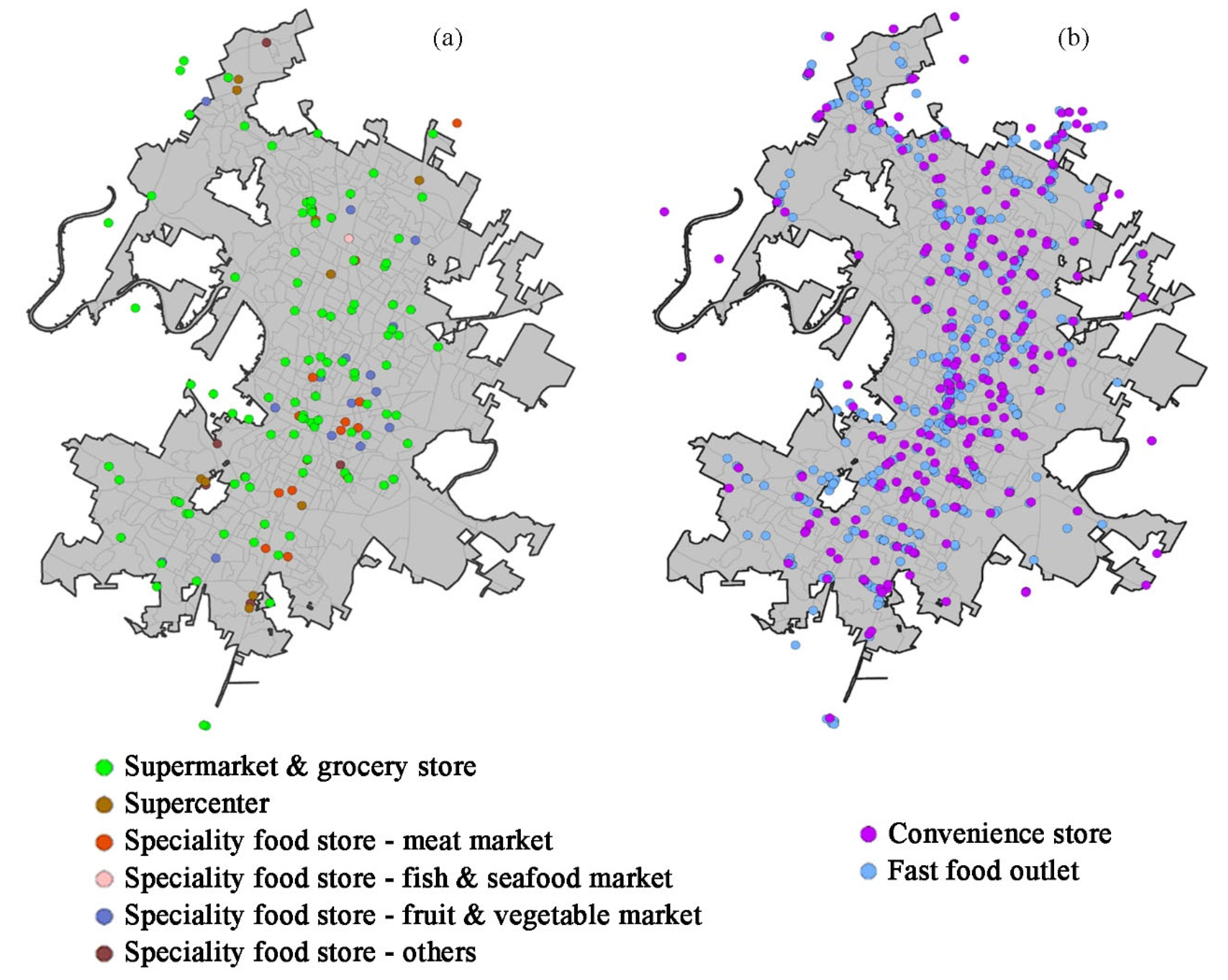
We geocoded the retail food stores’ data in ArcGIS 10.7. The mean geocoding matching scores ranged from 95.81% to 97.50%. We then projected the coordinate system to NAD 1983 UTM 14N. Van Meter et al. [53] recommended that any study involving accessibility measures should correct for edge effects. To do this, we created a 2000-m buffer around the Austin city boundary. Any stores within the buffer zone were kept for analysis. A total of 156 healthy food stores were identified in the Austin buffer zone—101 supermarkets and grocery stores, 14 supercenters, 14 meat markets, one fish and seafood market, 16 fruit and vegetable markets, and 10 other specialty food stores. Healthy food stores are mainly in the urban center along highway IH-35 (Figure 1a). A total of 245 convenience stores and 566 fast food outlets were geocoded (Figure 1b).
According to Kuai and Zhao who conducted food accessibility research in Baton Rouge, Louisiana [3], the business capacity of food stores can be estimated by the logarithm of the food store’s sales volume. We, therefore, adopted this logarithm transformation in our study. We coded the sales volume for each food outlet based on the upper limit of its “sales volume range” as reported by the data from ReferenceUSA. For instance, the sales volume range “<0.5 million” is assigned “500,000”. Details of the related data coding are shown in Table 1.
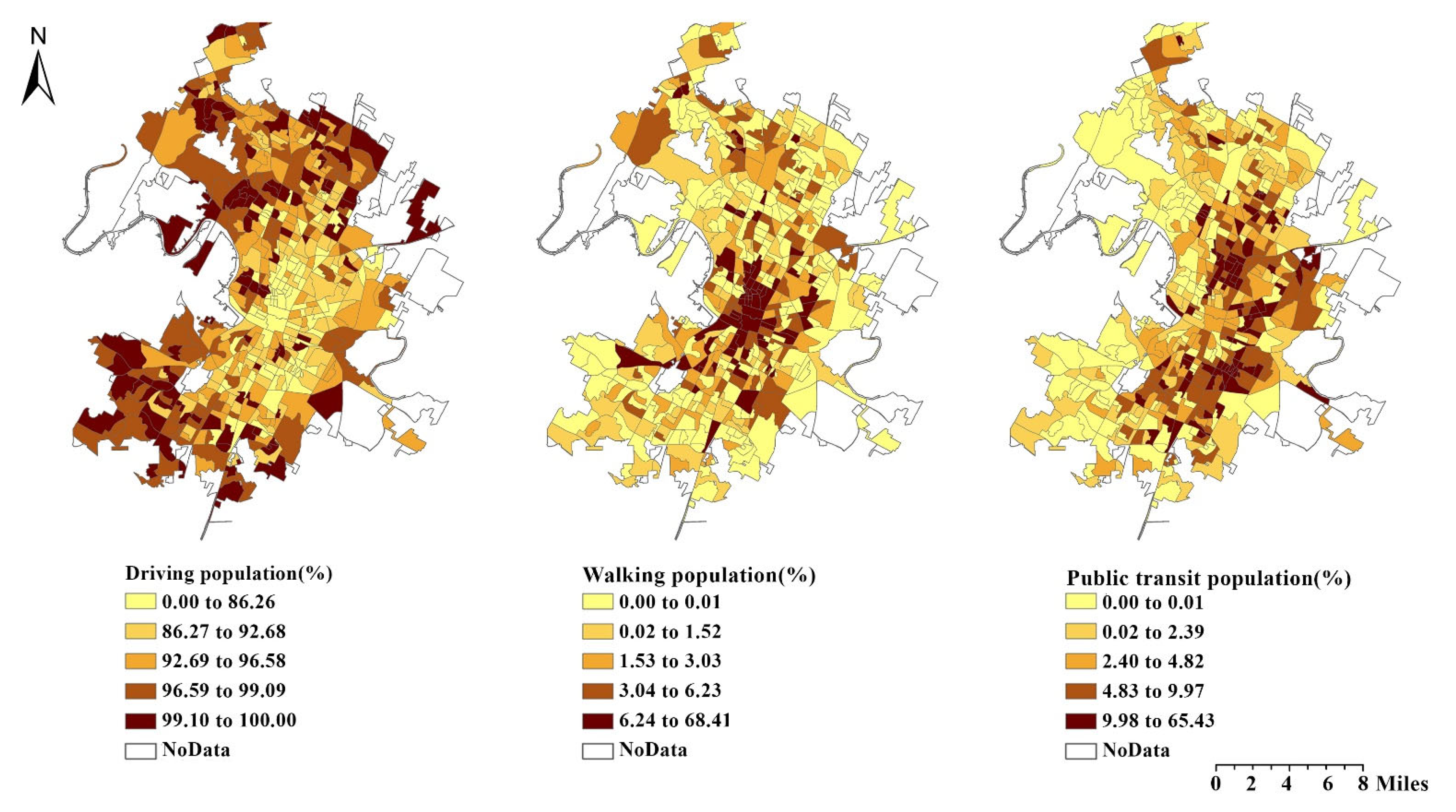
We considered three travel modes: driving, public transit, and walking; other modes, such as biking, motorcycling, and taxi, were not considered due to the lack of data availability and the limited adoption of these modes in general. However, whenever the data of the three travel modes were not available to use, we utilized transportation means to work data as surrogates. The transportation means to work data consists of information about different modes of commuting to work, such as driving, public transit, and walking, which were obtained from the 2016 American Community Survey (ACS) 5-year estimates. The number of people aged 25 to 64 years who used each transportation means (i.e., driving, public transit, and walking) in each census tract in Austin was extracted from the American Community Survey (ACS), and the percentages of population who utilized the three transportation modes were calculated (see Figure A1 in the Appendix A section). The driving and walking routes were calculated using road networks (see the Appendix A for setting up the travel network Figure A2). In terms of public transit, we used the General Transit Feed Specification (GTFS) to create public transit routes and to calculate the travel time between transit stops. We obtained the Austin GTFS containing the transit service for 1–30 June 2016 from the City of Austin website. Add GTFS to a Network Dataset, a toolkit developed by Melinda Morang and her team at ESRI, was used to convert GTFS text files to transit routes (see Figure A2 in the Appendix A section for the workflow of the conversion).
2.2. Method
2.2.1. Traditional 2SFCA Method
2SFCA [40]: This is the foundation of the two-step floating catchment area family. It has two critical steps. First, for each supply site j, all demand sites (k) in a catchment area are identified, and the supply-to-demand ratio within the catchment area () is calculated as follows:
where is the supply-to-demand ratio at supply site j that falls within the predefined catchment area ; is the capacity of supply at site j; is the travel time between site k and j; and is the population demand at site k that falls within the catchment.
Second, for each demand site i, all supply sites j that are within the catchment area are summed up for the supply-to-demand ratio as shown:
where is accessibility at location i; and or is the travel time between location i (or k) and j.
(Single-mode) Huff-based 2SFCA [10]: The 2SFCA method calculates the probability of people’s selection by only considering the travel time (or cost). Huff’s model quantifies the probability of people’s selection on a supply site when considering both travel cost and capacity of the supply site. The equation of the Huff model is:
where is the probability of population location i visiting supply site j based on the Huff model; is the travel cost from a population location i to supply site j; represent a given supply site and all supply sites within the catchment , respectively; denotes the travel cost from a population location i to all supply sites within the catchment; and β is the travel time impedance coefficient.
The first step of the Huff-based 2SFCA method is to utilize and a continuous negative power distance weight . The equation can be rewritten as:
The second step is to summarize at all supply sites within the catchment area . The equation is:
2.2.2. Multi-Mode Huff-Based 2SFCA
Inspired by Mao and Nekorchuk [48], we sought to improve the (single-mode) Huff-based 2SFCA model by incorporating multiple transport modes. We call this proposed method “multi-mode Huff-based 2SFCA”, which falls under the framework of 2SFCA. It utilizes different means of transportation as weights; then it assigns the weight for each mode of transportation to calculate the supply-to-demand ratio and the spatial accessibility index. It is implemented in three steps as described below.
First, it calculates the probability of people’s selection of a supply site based on different transportation modes. It considers both travel cost and capacity of the supply site simultaneously. The calculation resembles the one calculated in the Huff-based 2SFCA method. The difference is that the proposed method incorporates n () transportation modes into the equation. As a result, the equation is updated as:
where is the probability of population location i visiting supply site j based on the Huff model by transportation mode ; or is the travel time between i and j (or r) by transportation mode ; is the predefined travel catchment based on transportation mode ; r is any supply site within the catchment ; and β is the travel time impedance coefficient.
Second, the supply-to-demand ratio is calculated. At this step, n transportation modes is incorporated into Equation (4). Correspondingly, the population at location k is divided into n subpopulations by transportation modes [48], and the probability of people at population k selecting a supply site j is updated by transportation modes . Therefore, is rewritten as:
where is the travel time by the transportation mode between location k and j; is a predefined threshold travel time from j by mode ; is the Huff-model-based selection probability for the population at k to visit the supply site j by mode ; and is an inverse power impedance weight between k and j by mode .
Lastly, the overall accessibility at a population site is computed. The calculated in the second step at all supply sites by different transportation modes within the catchment is summarized. Instead of directly adding all within a catchment area, the multi-mode method assigns weighted values to each facility by the size of its subpopulation as per the catchment area(s) it falls within. Then, it sums the weighted values to calculate the overall accessibility (Ai) of the population i. The spatial accessibility should be the weighted average of accessibility of n subpopulation groups. The equation is:
where is the population at location i by transportation mode ; other notations remain the same as for Equation (7).
2.2.3. Comparison Analysis between Multi-Mode and Single-Mode Huff-Based 2SFCA
Multi-mode and single-mode Huff-based 2SFCA methods were compared using two methods: (1) a paired t-test was utilized to assess whether there is a significant difference between them; (2) the relative difference of each census-block group was computed to examine the magnitude and direction of the difference, and its equation is shown below [48]
where and are the spatial accessibility score for multi-mode and single-mode Huff-based 2SFCA methods, respectively.
We also examined whether the multiple- and single-mode measures were differentiated by vehicle ownership in each census tract. We obtained vehicle ownership data from the ACS and joined them to the census tract shapefile. Then, we calculated the percentage of households without vehicles in each census tract. Lastly, we separated the percentage of households without vehicles into two groups: more than or equal to 15%, and less than 15%, for the comparison of the spatial accessibility to food stores.
2.2.4. Implementation of Multi-Mode Huff-Based 2SFCA Method
Three catchments were used in our study: 10-min for walking [54], 15-min for driving, and 30 min for public transit [7]. In terms of setting up the network and travel time of each mode, please refer to Appendix A Figure A2 for more information. We first created an OD Cost Matrix, which computes the travel time of each travel mode for each census-block–food-outlet pair. For each population site, all the supply locations within its catchment area were identified by transportation mode and joined to the population site catchment layer. The drive-time properties were joined to calculate the Huff-based selection probability of a population location on supply sites within its catchment by different transportation modes. The calculation involves two factors: (1) the business capacity of a supply site; and (2) the inverse power drive-time weight ((travel time) ^(−β)) by transportation modes.
The second step computes the supply-to-demand ratio for each of the supply sites in the study area using Equation (7). For each supply site, all the population locations within its catchment area were identified by transportation mode and joined to the supply site catchment layer. The drive-time properties were joined to calculate the supply-to-demand ratio. The population demand was further adjusted by three factors: (1) the Huff-based selection weight; (2) the subpopulation groups by different modes; and (3) the inverse power drive-time weight ((travel time) ^ (−β)) by transportation modes.
The last step of the analysis sums the supply-to-demand ratios of each population location to calculate the accessibility using Equation (8). The overall accessibility was also adjusted by three factors: (1) the Huff-based selection probability of a population location on a supply site; (2) the subpopulation groups by different modes; and (3) the inverse power drive-time weight ((travel time) ^(−β)) by transportation modes.
The three steps all contain the impedance coefficient β. Luo [10] used six coefficients suggested by ESRI, ranging from 1.5 to 2.0. A wider range of coefficients, from 1.2 to 2.2 with an increment of 0.1, was employed to conduct the comparative analysis in our study.
3. Results
3.1. Geographic Access to Healthy and Unhealthy Food Outlets
Table 2 summarizes the statistics of the spatial accessibility index to healthy food outlets (SAIH) for census-block groups based on 11 different impedance coefficient (β) values. The maximum, mean, and standard deviation (SD) of the spatial accessibility index increase as the impedance coefficient increases, but the median of spatial accessibility index values decreases. The coefficient of variation (CV) increases as the impedance coefficient increases. All of these suggest that, as the impedance coefficient increases, the spatial accessibility to healthy food outlets diverges across the census-block groups in the study area. The Moran’s I-values of the spatial accessibility indices are positive and significant (p = 0.000) across the 11 impedance coefficient settings, indicating that the health food accessibility measures at block groups show positive spatial autocorrelation. The statistics of the spatial accessibility index to unhealthy food outlets (SAIU) show similar changing patterns to SAIH across the 11 impedance coefficient settings.
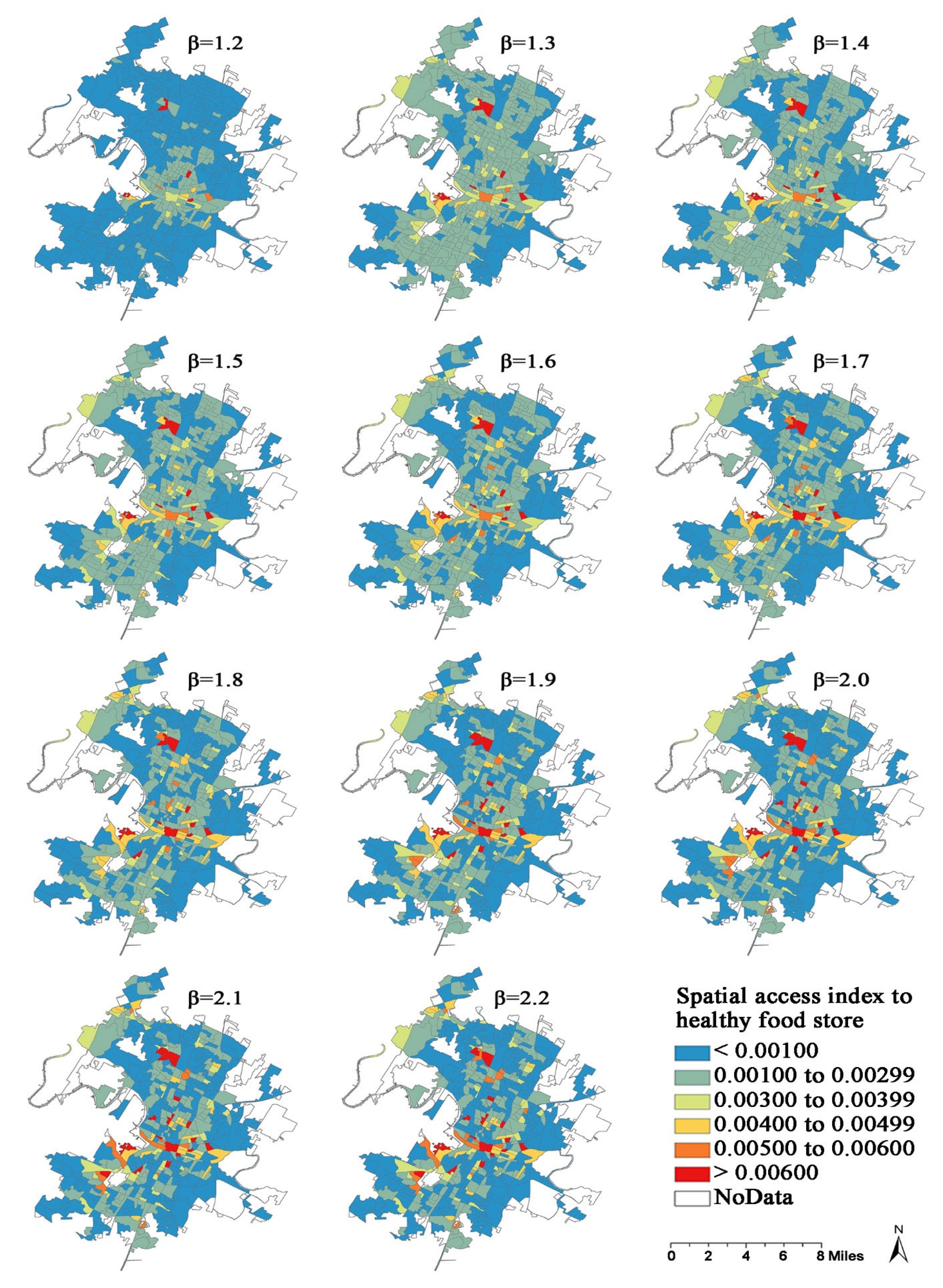
Figure 2 shows the spatial access to healthy food outlets with the distance impedance coefficient increasing from 1.2 to 2.2. A general trend is that the accessibility to healthy food outlets is high in the urban core and low in the peripheral areas of Austin. Put another way, spatial access to healthy foods decreases when moving away from the urban center. When the impedance coefficient is low (β = 1.2–1.4), and spatial autocorrelation is high, block groups with high spatial access to healthy foods are in the urban core and its surroundings. In contrast, low spatial accessibility is in the periphery of Austin. When the impedance coefficient is high (β = 1.8–2.2) and spatial autocorrelation is low, more census blocks outside the urban core area become dark-blue colored, indicating that more block groups in the periphery fall into the low accessibility interval. Meanwhile, more block groups in the inner urban area have higher accessibility values with a larger impedance coefficient. This intriguing pattern shows that increased impedance leads to high accessibility becoming higher and low accessibility lower, thus exacerbating food access disparity. This corroborates what is revealed by the CV values in Table 2, which shows an increasing trend in CV with larger impedance coefficients. Moreover, our model employed a wider range of impedance coefficients (from 1.2 to 2.2) than the single model [10] (i.e., 1.5 to 2.0); this not only helps identify in which coefficients the multiple- and single-mode models exhibit statistically significant differences, but it also shows more distinct disparities in terms of the spatial accessibility between urban cores, suburbs, and peripheries in Austin (as seen in Figure 2).
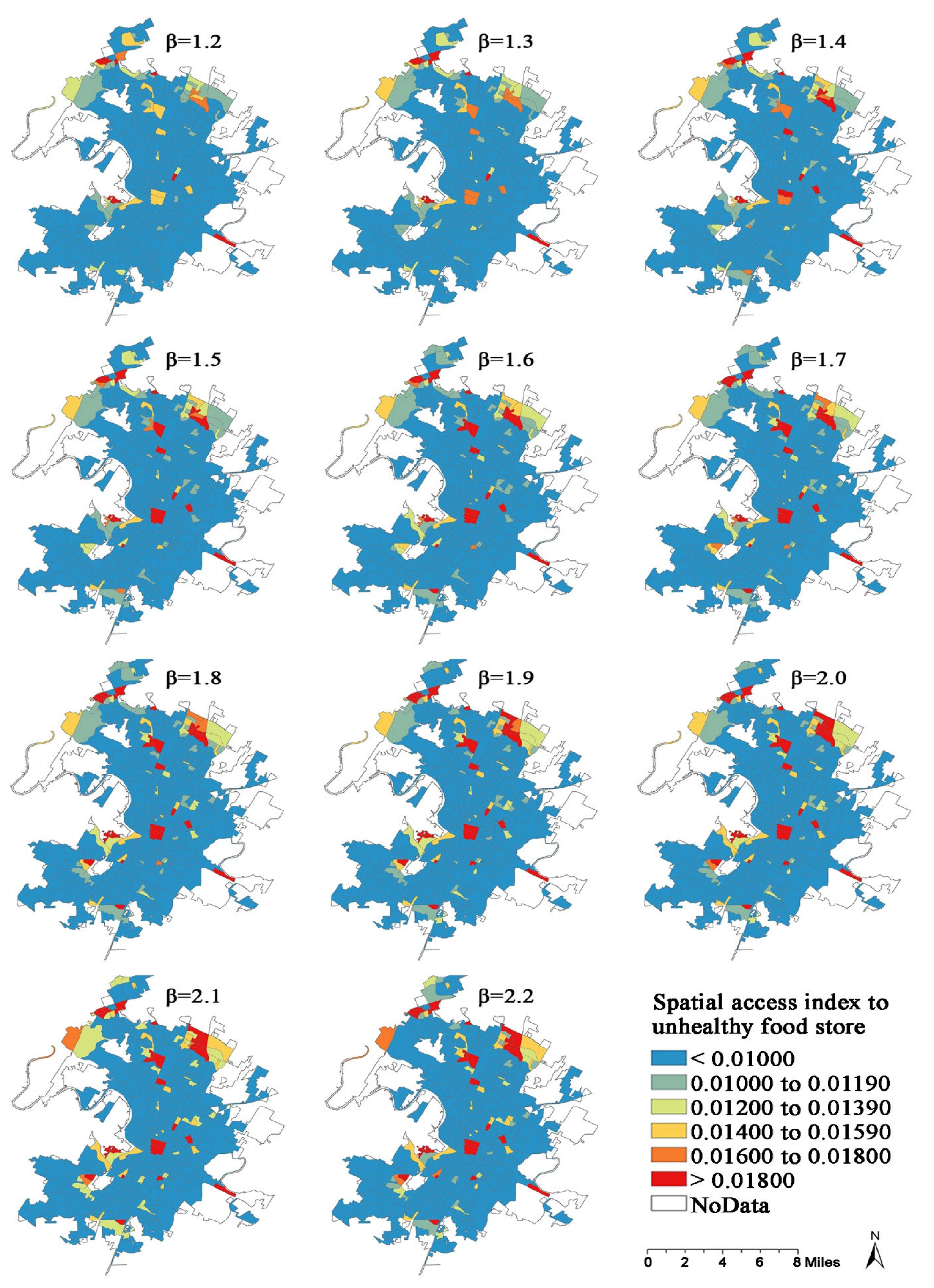
Accessibility to unhealthy food outlets (SAIU) in Austin is low in most of the block groups (Figure 3). High accessibility can be observed in a few block groups of the urban core and in the northwest and northeast of Austin. When the impedance coefficient is low (β = 1.2–1.5) and spatial autocorrelation is high, values in block groups with high accessibility become much higher as the impedance coefficient increases.
3.2. Results of the Comparison Analysis
Paired t-tests were conducted to compare the accessibility measurements to healthy food outlets using the multi-mode and single-mode Huff-based 2SFCA methods. It was found that in most cases, the two methods do not exhibit significant differences with different impedance coefficients (Table 3). There is only one exception; when equals 1.4. The mean difference of accessibility index between the two methods is largest at = 1.4, while the smallest mean difference is observed with values ranging from 1.9 to 2.2 (Table 3).
We also examined whether there is a significant difference between multi-mode and single-mode Huff-based 2SFCA methods for unhealthy food store accessibility. When equals 1.5, the two methods have a significant difference. The mean accessibility index values for the multi-mode are larger than the single model.
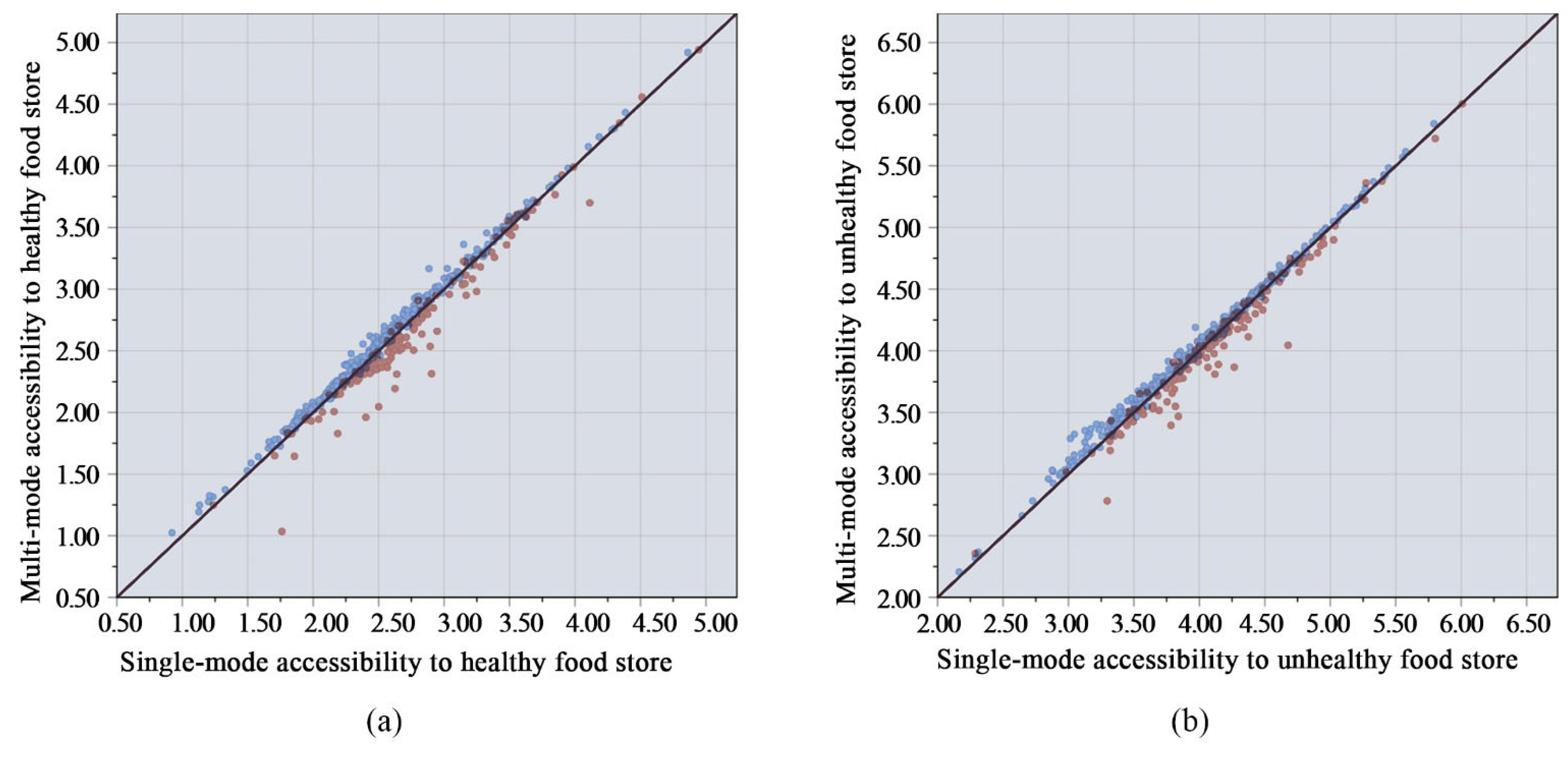
We further set the impedance coefficient β to 1.4 to compare healthy food accessibility measures (SAIH) between the multi-mode Huff-based 2SFCA method and the single-mode method. The original SAIH values were too small (as seen in Figure 2); for better illustration purposes, we multiplied the original SAIH values by 10,000 and applied a logarithm transformation to them. This showed that in areas with low vehicle ownership, the multi-mode tends to result in lower estimates than the single-mode (Figure 4a red dots). The difference is more noticeable when the accessibility value is medium (2.2–3.0). In contrast, in areas with low vehicle ownership, the multi-mode method predominantly generates a higher accessibility estimate than the single-mode method (Figure 4a blue dots). For the log-transformed values larger than 3.6, block groups with the multi-mode all have a higher estimate, leading to no estimations falling below the 1:1 reference line. We used the β value of 1.5 to compare the two modes for the unhealthy food accessibility measure (SAIU). In block groups where more than 15% of households were without vehicles (Figure 4b red dots), the multi-mode generally tends to result in lower estimation than the single-mode, showing the same pattern with the red dots in Figure 4a; this difference is quite marked when the log-transformed accessibility index is medium (3.7–4.5). In the remaining block groups where more than 85% of households have vehicles, the multi-mode method results in a higher estimation (Figure 4b blue dots). The difference is also notable when the transformed accessibility index is medium (3.0–4.0).
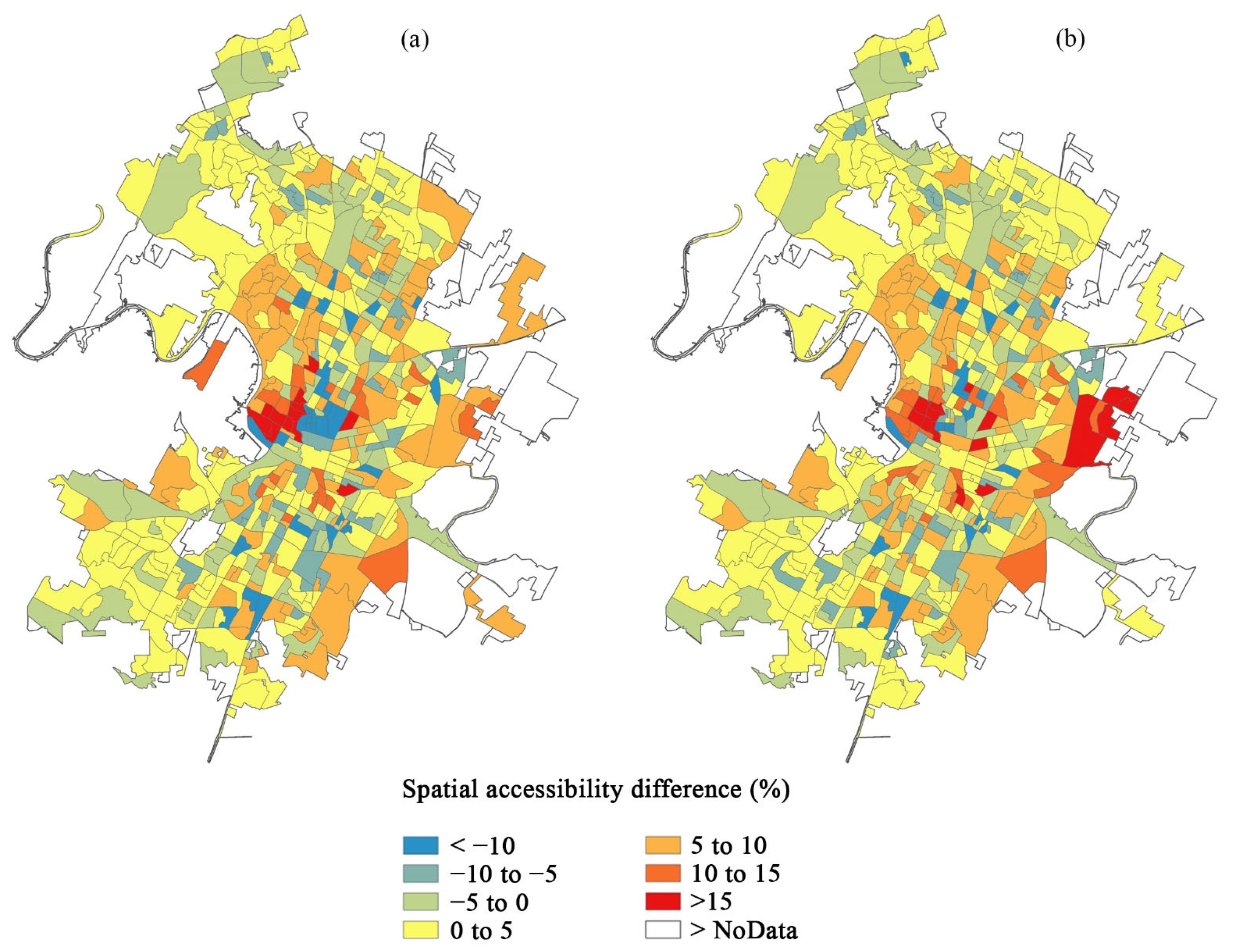
Figure 5a shows the magnitude and direction of the percentage difference between the two methods. In the urban center (i.e., downtown Austin and the University of Texas at Austin), the percentage difference is negative (<−10%), indicating that the accessibility index values by the multi-mode method are more than 10% lower than those by the single-mode method. In contrast, in most of the peripheral areas, the percentage difference is positive (0–10%). It suggests that the multi-mode method produced 0 to 10 percent higher accessibility index values than the single-mode one. We also observe that the block groups on the immediate west side of the downtown area are bright red in color (i.e., >15%, positive percent difference); these areas are geographically adjacent to the urban center. For the difference between the multiple- and single-mode methods in unhealthy food accessibility, a negative percent difference (<−10, or blue colors in Figure 5b) could be observed at the University of Texas at Austin (close to downtown Austin), as well as in the mid-north and mid-south of Austin along the IH-35, indicating that the multi-mode generates over 10% lower accessibility index values than its single-mode counterpart. In contrast, in most of the peripheral areas, the percentage differences are positive (0–10%). This suggests that the multi-mode method produces a <10% higher accessibility index than the single-mode method in these areas. Some block groups that approximate urban centers have a high positive percent difference (>15%) because most people (more than 96%) own personal vehicles and could drive to food stores for food shopping.
4. Discussion and Conclusions
A novel multi-mode Huff-based 2SFCA was proposed to overcome the disadvantages of the (single-mode) Huff-based 2SFCA. We applied the method in Austin, Texas, to measure both healthy and unhealthy food accessibility at the block-group level. It can effectively minimize the overestimation problem in urban areas. Therefore, it exhibits a more accurate picture of spatial access to food outlets than its alternatives.
With the proposed method, the spatial accessibility to both healthy and unhealthy food stores reveals a clear pattern in the urban core and peripheral areas. The urban core areas have the best access, whereas many block groups in peripheral regions in Austin have inadequate access to food stores. This result is consistent with previous findings [16]. Grocery stores, convenience stores, and other food outlets are mainly concentrated in urbanized areas [3]. Food retail businesses usually choose to operate in urban core areas because a dense population density in these areas can ensure high shopping volume and revenue [3]. However, some other food studies have a counterargument—for instance, “supermarket redlining” is a term used to describe the phenomenon of major supermarkets and grocery stores relocating their stores from inner-urban areas to suburbs [55], which is often connected with the formation of “food deserts” in the U.S and other developed countries [25,29,56]. On the contrary, the city of Austin did not have such developing patterns (as can be seen in Figure 1), and most of the chain grocery stores were still distributed in the inner urban area. The underlying reasons are worth further investigation in future studies.
We compared the proposed method with its single-mode alternative. The primary advantage of our approach is that it differentiates the population with and without vehicles. It uses different transportation modes as a constraint or weight to further adjust the overestimation demand in both steps, leading to a much more reasonable result than the single-model method. The two approaches are generally consistent with each other in terms of the urban core–peripheral disparities regardless of impedance coefficients. The results of the paired t-tests also support this finding because the two methods exhibit insignificant differences with most of the impedance coefficients (except for = 1.4 (healthy foods access) and = 1.5 (unhealthy foods access). We also found that the multi-mode method estimates an overall higher variability than the single-mode one; this is coincident with our expectation as a population with various transportation modes can maximize the heterogeneity of the measurement and thus produce a higher standard deviation.
In block groups with higher vehicle ownership (mostly in the peripheral Austin), the single-mode method produces a lower value than the multi-mode one. This can be explained as follows: The single mode assumes that all people drive vehicles to food outlets, leading to each food outlet serving more population in its catchment, which results in a larger denominator in Equation (4) and thus a lower supply-to-demand ratio Rj. At the last step of the single-mode method (Equation (5)), it sums all in its catchment. In peripheral areas, almost all households (more than 96%) have vehicles. There is not much difference between the single-mode (Equation (5)) and multiple-mode (Equation (8)) at this step. Because Rj tends to be lower in Equation (4), the single-mode method tends to generate lower accessibility indices in peripheral areas and underestimate the accessibility values. Therefore, the single-mode overestimates under-served areas for healthy food (e.g., 221.44 vs. 213.51 in Table 4), but underestimates over-served areas for unhealthy food (i.e., 80.30 vs. 83.25 in multi-mode in Table 4), in high vehicle-ownership block groups (the majority of which are in peripheral Austin). This finding is significant to food stakeholders and health policymakers for interventions. This finding indicates that when targeting interventions in peripheral Austin, stakeholders should be cautious if using the single-mode method because it asks for more intervening resources in under-served healthy food areas, but fewer resources in the over-served unhealthy food areas, than is actually needed.
For those block groups with lower vehicle ownership (mostly in inner Austin), the multi-mode method produces a lower value than the single-mode one, which could be explained as follows: The multi-mode method supposes that people procure foods by various transportation means, and thus fewer people compete for food, which results in a higher Rj (Equation (7)). In the urban core, a certain percentage (i.e., 20%) of people may not own a vehicle due to the availability of public transportation systems and severe traffic and parking issues. At the last step of the multi-mode method (Equation (8)), the lower driving percentage in urban areas impacts greatly on , and decreases the overall accessibility. As a result, the single-mode method produces a higher accessibility score than the multi-mode one in inner Austin. Despite this, in most of the inner Austin, the single-mode method tends to underestimate the under-served healthy food areas (e.g., 20.53 vs. 24.19 in Table 4) and overestimate the over-served unhealthy food areas (e.g., 15.62 vs. 14.89 in Table 4).
Despite the advantages of the proposed method, the results should be interpreted with caution. Firstly, the cut-off travel time to define the different service zones (e.g., 10-min walking, 15-min driving, and 30-min public transit) in this study was based on empirical data. For future studies, a customer survey may be needed to determine the most appropriate traveling time to define the catchment size for each transportation mode [57]. Moreover, the catchment size could vary for different applications based on neighborhood characteristics and context [39]. Secondly, we assume that home-to-store travel is the way most people access food stores. But people do not always travel from home to food outlets. Food trips may be a part of their multi-purpose trip involving journey-to-work, journey-to-entertainment, etc. Lastly, here we only considered spatial disadvantage (i.e., where food outlets are) to quantify neighborhoods’ accessibility to foods since this is primarily a spatial accessibility study. However, non-spatial sociodemographic factors are equally essential to identify food access challenges.
Author Contributions
He Jin: Conceptualization, Methodology, Formal analysis, Software, Data curation, Visualization, Validation, Writing-Original draft preparation; Yongmei Lu: Supervision, Writing-Reviewing, and Editing. All authors have read and agreed to the published version of the manuscript.
Funding
This research received no external funding.
Data Availability Statement
The survey data are available upon request from the corresponding author.
Conflicts of Interest
The authors declare no conflict of interest.
Appendix A
Figure A1.
Percentage of population with three transportation modes to work in Austin, Tx.

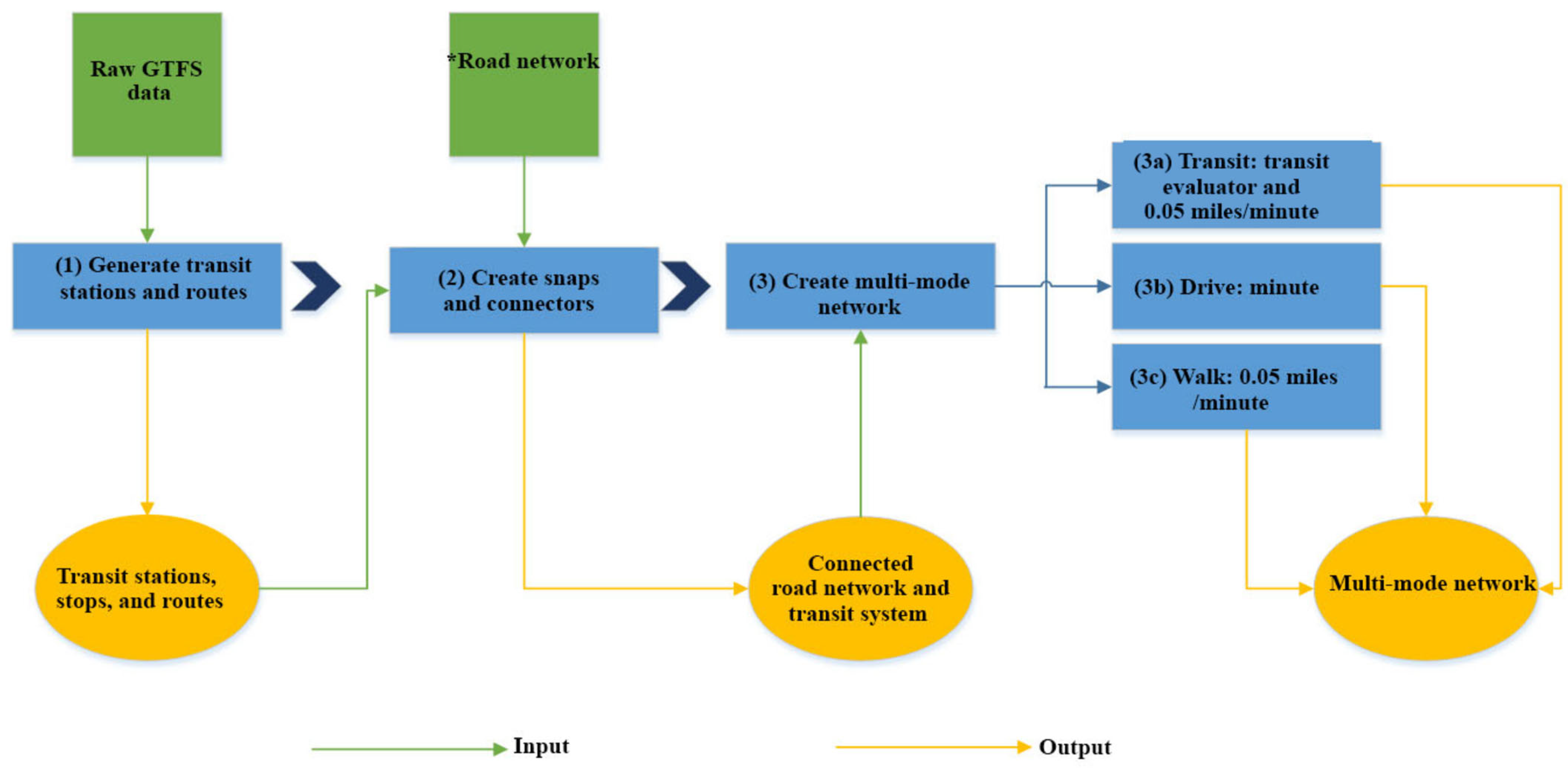
Figure A2.
Steps to create a multi-mode network using GTFS text file and road network. Note: * Road network includes interstate, freeway, expressway, toll, U.S. and state highways, major arterials, country roads, minor arterials, country streets, ramps and turnarounds, driveways, service roads, private road, platted row/unbuilt, sidewalks, and walkways.

Figure A2 shows the steps to create a multi-mode network and calculate travel times for the three travel modes. The description of the configuration is shown below.
- (1)
- Generate transit routes and stations. GTFS text file contains latitude/longitude information of transit stations, and this information is read by Generate transit lines and stops tool in Add GTFS Data to a Network Dataset toolkit embedded in ArcGIS. A point shapefile that contains all transit stops in Austin is created to store spatial information. Then it generates straight lines to connect two adjacent stops; lines are converted to line shapefiles (i.e., transit routes). In total, 2684 transit stops and 3232 transit route segments were generated.
- (2)
- Create connectors between transit stops to street networks. Road networks and transit stops (or transit lines) come from different resources; there might be gaps between transit stops and road networks. People can’t cross the gaps unless there is a “bridge” connecting transit stops and streets. The Generate Stop-Street Connectors tool can create a “connector” as a “bridge” to facilitate pedestrians to walk through. The “connector” is a short straight line and is perpendicular to streets, and it connects the transit system and street network. The “connector” might not exist in the real world but is an important step. By creating connectors, transit lines and street networks only are connected at stops, which prevents pedestrians from walking on transit lines.
- (3)
- Create a multi-mode transportation network. With the creating a multi-mode network dataset toolkit provided in ArcGIS 10.8 Network Analyst Extension, a multi-mode transit network could be created. The setup of three transportation modes is shown below.
(3a) Transit mode. There is an assumption that people walk on the street to transit stops, then take transits to other transit stops to get off and walk on street lines to arrive at destinations. We assume an ingress, egress, and transfer with a walking speed of 0.05 miles/minute. For the connectors created in step 2, we apply a delay of 0.5 min for transitions between streets and transit lines (to represent boarding a transit vehicle) and a delay of 0.5 min for transitions from transit lines to streets (to represent alighting). We also create a pedestrian restriction to prevent pedestrians from walking on four types of roads: 1 (interstate, freeway, expressway, and toll), 2 (U.S. and state highways), 15 (private road), and 17 (platted row/unbuilt). The evaluator is vital for setting up the network because it determines how the network uses the fields in shapefile tables. For transit networks, we use a transit evaluator from the add GTFS to a network dataset toolkit to calculate transit travel time along transit lines. The transit evaluator determines the travel time across that transit line by looking up the available transit trips in the GTFS schedules at the appropriate time of day and summing the wait time for the trip plus the ride time from the current stop to the next. In our analysis, we used a general Monday to calculate the transit travel time because we were not focusing on a specific timetable or schedule of the transits. A general workday like Monday can serve the analysis.
(3b) Drive mode. The setup of the drive mode is not as complex as the transit mode. The street shapefile has a field “minutes”, which is the minimum travel time on each street segment. The evaluator uses the “minutes” to calculate drive time on the street. In addition, the evaluator uses a one-way (such as “B”, “FT”, and “TF”) field in the street shapefile as a one-way restriction.
(3c) Walk mode. The setup of walk mode is identical to the pedestrian part of transit mode. We assume that the walking speed is 0.05 miles/min.
References
- Glanz, K.; Sallis, J.F.; Saelens, B.E.; Frank, L.D. Healthy nutrition environments: Concepts and measures. Am. J. Health Promot. 2005, 19, 330–333. [Google Scholar] [CrossRef]
- Luan, H. Spatial and Spatio-Temporal Analyses of Neighborhood Retail Food Environments: Evidence for Food Planning and Interventions. UWSpace. 2016. Available online: http://hdl.handle.net/10012/11079 (accessed on 21 June 2017).
- Kuai, X.; Zhao, Q. Examining healthy food accessibility and disparity in Baton Rouge, Louisiana. Ann. GIS 2017, 23, 103–116. [Google Scholar] [CrossRef]
- Wang, F.; Luo, W. Assessing spatial and nonspatial factors for healthcare access: Towards an integrated approach to defining health professional shortage areas. Health Place 2005, 11, 131–146. [Google Scholar] [CrossRef]
- Thornton, R.L.; Glover, C.M.; Cené, C.W.; Glik, D.C.; Henderson, J.A.; Williams, D.R. Evaluating strategies for reducing health disparities by addressing the social determinants of health. Health Aff. 2016, 35, 1416–1423. [Google Scholar] [CrossRef] [Green Version]
- Algert, S.J.; Agrawal, A.; Lewis, D.S. Disparities in access to fresh produce in low-income neighborhoods in Los Angeles. Am. J. Prev. Med. 2006, 30, 365–370. [Google Scholar] [CrossRef]
- Dai, D.; Wang, F. Geographic disparities in accessibility to food stores in southwest Mississippi. Environ. Plan. B Plan. Des. 2011, 38, 659–677. [Google Scholar] [CrossRef]
- O’Dwyer, L.A.; Burton, D.L. Potential meets reality: GIS and public health research in Australia. Aust. N. Z. J. Public Health 1998, 22, 819–823. [Google Scholar] [CrossRef]
- Langford, M.; Higgs, G. Measuring potential access to primary healthcare services: The influence of alternative spatial representations of population. Prof. Geogr. 2006, 58, 294–306. [Google Scholar] [CrossRef]
- Luo, J. Integrating the Huff model and floating catchment area methods to analyze spatial access to healthcare services. Trans. GIS 2014, 18, 436–448. [Google Scholar] [CrossRef]
- Charreire, H.; Casey, R.; Salze, P.; Simon, C.; Chaix, B.; Banos, A.; Badariotti, D.; Weber, C.; Oppert, J.-M. Measuring the food environment using geographical information systems: A methodological review. Public Health Nutr. 2010, 13, 1773–1785. [Google Scholar] [CrossRef]
- Forsyth, A.; Lytle, L.; Van Riper, D. Finding food: Issues and challenges in using Geographic Information Systems to measure food access. J. Transp. Land Use 2010, 3, 43. [Google Scholar] [CrossRef]
- Hilmers, A.; Hilmers, D.C.; Dave, J. Neighborhood disparities in access to healthy foods and their effects on environmental justice. Am. J. Public Health 2012, 102, 1644–1654. [Google Scholar] [CrossRef]
- Block, J.P.; Scribner, R.A.; DeSalvo, K.B. Fast food, race/ethnicity, and income. Am. J. Prev. Med. 2004, 27, 211–217. [Google Scholar] [CrossRef]
- Winkler, E.; Turrell, G.; Patterson, C. Does living in a disadvantaged area mean fewer opportunities to purchase fresh fruit and vegetables in the area? Findings from the Brisbane food study. Health Place 2006, 12, 306–319. [Google Scholar] [CrossRef]
- Apparicio, P.; Cloutier, M.-S.; Shearmur, R. The case of Montreal’s missing food deserts: Evaluation of accessibility to food supermarkets. Int. J. Health Geogr. 2007, 6, 4. [Google Scholar] [CrossRef] [Green Version]
- Austin, S.B.; Melly, S.J.; Sanchez, B.N.; Patel, A.; Buka, S.; Gortmaker, S.L. Clustering of fast-food restaurants around schools: A novel application of spatial statistics to the study of food environments. Am. J. Public Health 2005, 95, 1575–1581. [Google Scholar] [CrossRef]
- Baker, E.A.; Schootman, M.; Barnidge, E.; Kelly, C. Peer reviewed: The role of race and poverty in access to foods that enable individuals to adhere to dietary guidelines. Prev. Chronic Dis. 2006, 3, A76. [Google Scholar]
- Powell, L.M.; Chaloupka, F.J.; Bao, Y. The availability of fast-food and full-service restaurants in the United States: Associations with neighborhood characteristics. Am. J. Prev. Med. 2007, 33, S240–S245. [Google Scholar] [CrossRef]
- Moore, L.V.; Diez Roux, A.V.; Nettleton, J.A.; Jacobs, D.R., Jr. Associations of the local food environment with diet quality—A comparison of assessments based on surveys and geographic information systems: The multi-ethnic study of atherosclerosis. Am. J. Epidemiol. 2008, 167, 917–924. [Google Scholar] [CrossRef] [Green Version]
- Wang, M.C.; Kim, S.; Gonzalez, A.A.; MacLeod, K.E.; Winkleby, M.A. Socioeconomic and food-related physical characteristics of the neighbourhood environment are associated with body mass index. J. Epidemiol. Community Health 2007, 61, 491–498. [Google Scholar] [CrossRef] [Green Version]
- Zenk, S.N.; Schulz, A.J.; Israel, B.A.; James, S.A.; Bao, S.; Wilson, M.L. Neighborhood racial composition, neighborhood poverty, and the spatial accessibility of supermarkets in metropolitan Detroit. Am. J. Public Health 2005, 95, 660–667. [Google Scholar] [CrossRef]
- Wang, F. Quantitative Methods and Socio-Economic Applications in GIS; CRC Press: Boca Raton, FL, USA, 2014. [Google Scholar]
- D’Acosta, J. Finding Food Deserts: A Study of Food Access Measures in the Phoenix-Mesa Urban Area; University of Southern California: Los Angeles, CA, USA, 2015. [Google Scholar]
- Larsen, K.; Gilliland, J. Mapping the evolution of ’food deserts’ in a Canadian city: Supermarket accessibility in London, Ontario, 1961–2005. Int. J. Health Geogr. 2008, 7, 16. [Google Scholar] [CrossRef] [Green Version]
- Opfer, P.R. Using GIS Technology to Identify and Analyze ‘Food Deserts’ on the Southern Oregon Coast. 2010. Available online: https://ir.library.oregonstate.edu/concern/graduate_projects/xd07gv654 (accessed on 15 September 2018).
- Pearce, J.; Blakely, T.; Witten, K.; Bartie, P. Neighborhood deprivation and access to fast-food retailing: A national study. Am. J. Prev. Med. 2007, 32, 375–382. [Google Scholar] [CrossRef]
- Sharkey, J.R.; Horel, S.; Dean, W.R. Neighborhood deprivation, vehicle ownership, and potential spatial access to a variety of fruits and vegetables in a large rural area in Texas. Int. J. Health Geogr. 2010, 9, 26. [Google Scholar] [CrossRef] [Green Version]
- Sparks, A.L.; Bania, N.; Leete, L. Comparative approaches to measuring food access in urban areas: The case of Portland, Oregon. Urban Stud. 2011, 48, 1715–1737. [Google Scholar] [CrossRef]
- Gallagher, M.J.C. Examining the Impact of Food Deserts on Public Health in Detroit; Mari Gallagher Research and Consulting Group: Chicago, IL, USA, 2007. [Google Scholar]
- Wan, N.; Zou, B.; Sternberg, T. A three-step floating catchment area method for analyzing spatial access to health services. Int. J. Geogr. Inf. Sci. 2012, 26, 1073–1089. [Google Scholar] [CrossRef]
- Guagliardo, M.F. Spatial accessibility of primary care: Concepts, methods and challenges. Int. J. Health Geogr. 2004, 3, 3. [Google Scholar] [CrossRef] [Green Version]
- Joseph, A.E.; Bantock, P.R. Measuring potential physical accessibility to general practitioners in rural areas: A method and case study. Soc. Sci. Med. 1982, 16, 85–90. [Google Scholar] [CrossRef]
- Chen, X.; Clark, J. Measuring space–time access to food retailers: A case of temporal access disparity in Franklin County, Ohio. Prof. Geogr. 2016, 68, 175–188. [Google Scholar] [CrossRef]
- Zenk, S.N.; Schulz, A.J.; Matthews, S.A.; Odoms-Young, A.; Wilbur, J.; Wegrzyn, L.; Gibbs, K.; Braunschweig, C.; Stokes, C. Activity space environment and dietary and physical activity behaviors: A pilot study. Health Place 2011, 17, 1150–1161. [Google Scholar] [CrossRef] [Green Version]
- Shannon, J. Beyond the supermarket solution: Linking food deserts, neighborhood context, and everyday mobility. Ann. Am. Assoc. Geogr. 2016, 106, 186–202. [Google Scholar] [CrossRef]
- Balstrøm, T. On identifying the most time-saving walking route in a trackless mountainous terrain. Geogr. Tidsskr.-Dan. J. Geogr. 2002, 102, 51–58. [Google Scholar] [CrossRef]
- Sherrill, K.; Frakes, B.; Schupbach, S. Travel Time Cost Surface Model: Standard Operating Procedure; Natural Resource Report. Nps/Nrpc/Imd/Nrr–2010/238. Published Report-2164894; Natural Resources Program Center: Fort Collins, CO, USA, 2010. [Google Scholar]
- Wan, N.; Zhan, F.B.; Zou, B.; Chow, E. A relative spatial access assessment approach for analyzing potential spatial access to colorectal cancer services in Texas. Appl. Geogr. 2012, 32, 291–299. [Google Scholar] [CrossRef]
- Luo, W.; Wang, F. Measures of spatial accessibility to health care in a GIS environment: Synthesis and a case study in the Chicago region. Environ. Plan. B Plan. Des. 2003, 30, 865–884. [Google Scholar] [CrossRef] [Green Version]
- Vo, A.; Plachkinova, M.; Bhaskar, R. Assessing healthcare accessibility algorithms: A comprehensive investigation of two-step floating catchment methodologies family. In Proceedings of the 2015 Americas Conferences on Information Systems (AMCIS 2015), Fajardo, Puerto Rico, 13–15 August 2015; p. 17. [Google Scholar]
- Lin, Y.; Wan, N.; Sheets, S.; Gong, X.; Davies, A. A multi-modal relative spatial access assessment approach to measure spatial accessibility to primary care providers. Int. J. Health Geogr. 2018, 17, 33. [Google Scholar] [CrossRef] [Green Version]
- Park, J.; Goldberg, D.W. A review of recent spatial accessibility studies that benefitted from advanced geospatial information: Multimodal transportation and spatiotemporal disaggregation. ISPRS Int. J. Geo-Inf. 2021, 10, 532. [Google Scholar] [CrossRef]
- Tao, Z.; Zhou, J.; Lin, X.; Chao, H.; Li, G.J. Investigating the impacts of public transport on job accessibility in Shenzhen, China: A multi-modal approach. Land Use Policy 2020, 99, 105025. [Google Scholar] [CrossRef]
- Zhou, X.; Yu, Z.; Yuan, L.; Wang, L.; Wu, C.J. Measuring accessibility of healthcare facilities for populations with multiple transportation modes considering residential transportation mode choice. ISPRS Int. J. Geo-Inf. 2020, 9, 394. [Google Scholar] [CrossRef]
- Tao, Z.; Yao, Z.; Kong, H.; Duan, F.; Li, G.J. Spatial accessibility to healthcare services in Shenzhen, China: Improving the multi-modal two-step floating catchment area method by estimating travel time via online map APIs. BMC Health Serv. Res. 2018, 18, 345. [Google Scholar] [CrossRef] [Green Version]
- Hu, S.; Song, W.; Li, C.; Lu, J.J.C. A multi-mode Gaussian-based two-step floating catchment area method for measuring accessibility of urban parks. Cities 2020, 105, 102815. [Google Scholar] [CrossRef]
- Mao, L.; Nekorchuk, D. Measuring spatial accessibility to healthcare for populations with multiple transportation modes. Health Place 2013, 24, 115–122. [Google Scholar] [CrossRef]
- Huff, D.L.J.E. ArcUser. Parameter Estimation in the Huff Model. 2003, pp. 34–36. Available online: https://www.esri.com/news/arcuser/1003/files/huff.pdf (accessed on 23 August 2022).
- Jin, H.; Lu, Y. Evaluating consumer nutrition environment in food deserts and food swamps. Int. J. Environ. Res. Public Health 2021, 18, 2675. [Google Scholar] [CrossRef]
- Jin, H.; Lu, Y. SAR-Gi*: Taking a spatial approach to understand food deserts and food swamps. Appl. Geogr. 2021, 134, 102529. [Google Scholar] [CrossRef]
- Stein, D.O. ‘Food Deserts’ and ‘Food Swamps’ in Hillsborough County, Florida: Unequal Access to Supermarkets and Fast-Food Restaurants; University of South Florida: Tampa, FL, USA, 2011. [Google Scholar]
- Van Meter, E.M.; Lawson, A.B.; Colabianchi, N.; Nichols, M.; Hibbert, J.; Porter, D.E.; Liese, A.D. An evaluation of edge effects in nutritional accessibility and availability measures: A simulation study. Int. J. Health Geogr. 2010, 9, 40. [Google Scholar] [CrossRef] [Green Version]
- Yang, Y.; Diez-Roux, A.V. Using an agent-based model to simulate children’s active travel to school. Int. J. Behav. Nutr. Phys. Act. 2013, 10, 67. [Google Scholar] [CrossRef] [Green Version]
- Zhang, M.; Ghosh, D. Spatial Supermarket Redlining and Neighborhood Vulnerability: A Case Study of Hartford, Connecticut. Trans. GIS 2016, 20, 79–100. [Google Scholar] [CrossRef] [Green Version]
- Whelan, A.; Wrigley, N.; Warm, D.; Cannings, E.J.U.S. Life in a ‘food desert’. Urban Stud. 2002, 39, 2083–2100. [Google Scholar] [CrossRef]
- Wan, N.; Zhan, F.B.; Zou, B.; Wilson, J.G. Spatial access to health care services and disparities in colorectal cancer stage at diagnosis in Texas. Prof. Geogr. 2013, 65, 527–541. [Google Scholar] [CrossRef]
Figure 1.
Healthy (a) and unhealthy (b) food outlets in Austin, TX [51].
Figure 1.
Healthy (a) and unhealthy (b) food outlets in Austin, TX [51].

Figure 2.
Spatial distribution of the SAIH at the census-block group level for a range of impedance coefficients.
Figure 2.
Spatial distribution of the SAIH at the census-block group level for a range of impedance coefficients.

Figure 3.
Spatial distribution of the SAIU at the census-block group level for a range of impedance coefficients.
Figure 3.
Spatial distribution of the SAIU at the census-block group level for a range of impedance coefficients.

Figure 4.
Comparison of the multi-mode and single-mode Huff-based 2SFCA in block groups with more than (or equal to) 15% (red dots) vs. less than 15% households without vehicles (blue dots) for (a) Ln SAIH and (b) Ln SAIU.
Figure 4.
Comparison of the multi-mode and single-mode Huff-based 2SFCA in block groups with more than (or equal to) 15% (red dots) vs. less than 15% households without vehicles (blue dots) for (a) Ln SAIH and (b) Ln SAIU.

Figure 5.
Relative differences between the multi-mode and single-mode Huff-based 2SFCA on (a) SAIH and (b) SAIU.
Figure 5.
Relative differences between the multi-mode and single-mode Huff-based 2SFCA on (a) SAIH and (b) SAIU.


Table 1.
Business capacity of food stores in the study area.
| Sales Volume Range | Sales Volume | Store Capacity | The Number of Healthy Food Stores | The Number of Unhealthy Food Stores |
|---|---|---|---|---|
| <0.5 million | 500,000 | 5.69 | 15 | 128 |
| 0.5~1.0 million | 1,000,000 | 6.00 | 9 | 234 |
| 1.0~2.5 million | 2,500,000 | 6.39 | 36 | 385 |
| 2.5~5 million | 5,000,000 | 6.69 | 13 | 61 |
| 5~10 million | 10,000,000 | 7.00 | 11 | 1 |
| 10~20 million | 20,000,000 | 7.30 | 8 | 2 |
| 20~50 million | 50,000,000 | 7.69 | 35 | NA |
| 50~100 million | 100,000,000 | 8.00 | 24 | NA |
| 100~500 million | 500,000,000 | 8.69 | 5 | NA |
Table 2.
Descriptive statistics of the SAIH.
| β | Min | 1st Quartile | Median | 3rd Quartile | Max | Mean | SD | CV | Moran’s I |
|---|---|---|---|---|---|---|---|---|---|
| 1.2 | 0.00023 | 0.00111 | 0.00139 | 0.00188 | 0.01047 | 0.00168 | 0.00110 | 0.65451 | 0.09493 |
| 1.3 | 0.00019 | 0.00104 | 0.00134 | 0.00189 | 0.01213 | 0.00170 | 0.00126 | 0.74160 | 0.07861 |
| 1.4 | 0.00015 | 0.00096 | 0.00129 | 0.00191 | 0.01400 | 0.00171 | 0.00143 | 0.83982 | 0.07153 |
| 1.5 | 0.00012 | 0.00089 | 0.00124 | 0.00195 | 0.01506 | 0.00171 | 0.00153 | 0.89320 | 0.06990 |
| 1.6 | 0.00010 | 0.00083 | 0.00121 | 0.00198 | 0.01622 | 0.00172 | 0.00165 | 0.95570 | 0.06644 |
| 1.7 | 0.00008 | 0.00077 | 0.00116 | 0.00198 | 0.01718 | 0.00173 | 0.00175 | 1.01175 | 0.06312 |
| 1.8 | 0.00006 | 0.00071 | 0.00111 | 0.00200 | 0.01796 | 0.00174 | 0.00184 | 1.06173 | 0.06005 |
| 1.9 | 0.00005 | 0.00066 | 0.00106 | 0.00204 | 0.01859 | 0.00174 | 0.00192 | 1.10559 | 0.05734 |
| 2.0 | 0.00004 | 0.00061 | 0.00103 | 0.00207 | 0.01910 | 0.00175 | 0.00200 | 1.14446 | 0.05492 |
| 2.1 | 0.00003 | 0.00057 | 0.00099 | 0.00212 | 0.01952 | 0.00175 | 0.00206 | 1.17961 | 0.05268 |
| 2.2 | 0.00002 | 0.00053 | 0.00096 | 0.00216 | 0.01989 | 0.00175 | 0.00212 | 1.21151 | 0.05061 |
Table 3.
The paired t-test between the multi-mode and single-mode methods regarding the SAIH.
| Paired Difference a | ||||||
|---|---|---|---|---|---|---|
| β | Mean | Stand Deviation | Standard Error | 95% Confidence Interval of the Difference | t-Value | p-Value |
| 1.2 | 0.000013 | 0.000189 | 0.000009 | (−0.000004, 0.000030) | 1.526 | 0.128 |
| 1.3 | 0.000012 | 0.000186 | 0.000009 | (−0.000004, 0.000029) | 1.452 | 0.147 |
| 1.4 | 0.000013 | 0.000125 | 0.000006 | (0.000002, 0.000024) | 1.981 | 0.048 * |
| 1.5 | 0.000009 | 0.000175 | 0.000008 | (−0.000007, 0.000025) | 1.151 | 0.25 |
| 1.6 | 0.000010 | 0.000166 | 0.000008 | (−0.000005, 0.000025) | 1.303 | 0.193 |
| 1.7 | 0.000009 | 0.000159 | 0.000007 | (−0.000005, 0.000023) | 1.260 | 0.208 |
| 1.8 | 0.000008 | 0.000152 | 0.000007 | (−0.000006, 0.000022) | 1.124 | 0.262 |
| 1.9 | 0.000007 | 0.000146 | 0.000007 | (−0.000006, 0.000021) | 1.111 | 0.267 |
| 2.0 | 0.000007 | 0.00014 | 0.000006 | (−0.000005, 0.000020) | 1.155 | 0.249 |
| 2.1 | 0.000007 | 0.000136 | 0.000006 | (−0.000005, 0.000019) | 1.132 | 0.258 |
| 2.2 | 0.000007 | 0.000131 | 0.000006 | (−0.000005, 0.000018) | 1.081 | 0.280 |
Note: * significant at 0.05 level; a: statistics of paired difference are multi-mode Huff-based 2SFCA minus the single-mode Huff-based 2SFCA.
Table 4.
Comparison of using the single-mode and multi-mode methods to estimate food service areas.
| Vehicle Ownership | Method | Under-Served Area for Healthy Food (km2) a | Under-Served Population for Healthy Food a | Over-Served Area for Unhealthy Food (km2) b | Over-Served Population for Unhealthy Food b |
|---|---|---|---|---|---|
| Block groups with high vehicle ownership | Single-mode | 221.44 | 185,606 | 80.30 | 79,778 |
| Multi-mode | 213.51 | 175,399 | 83.25 | 83,168 | |
| Block groups with low vehicle ownership | Single-mode | 20.53 | 38,205 | 15.62 | 32,053 |
| Multi-mode | 24.19 | 47,263 | 14.89 | 28,007 |
Note: a the under-served area is defined as the spatial accessibility to healthy food lower than 1 supermarket/grocery store per 1000 people; b the over-served area is defined as the spatial accessibility to unhealthy food higher than 10 convenience stores & fast-food outlets per 1000 people.
Publisher’s Note: MDPI stays neutral with regard to jurisdictional claims in published maps and institutional affiliations. |
© 2022 by the authors. Licensee MDPI, Basel, Switzerland. This article is an open access article distributed under the terms and conditions of the Creative Commons Attribution (CC BY) license (https://creativecommons.org/licenses/by/4.0/).
Share and Cite
MDPI and ACS Style
Jin, H.; Lu, Y. Multi-Mode Huff-Based 2SFCA: Examining Geographical Accessibility to Food Outlets in Austin, Texas. ISPRS Int. J. Geo-Inf. 2022, 11, 579. https://doi.org/10.3390/ijgi11110579
AMA Style
Jin H, Lu Y. Multi-Mode Huff-Based 2SFCA: Examining Geographical Accessibility to Food Outlets in Austin, Texas. ISPRS International Journal of Geo-Information. 2022; 11(11):579. https://doi.org/10.3390/ijgi11110579
Chicago/Turabian StyleJin, He, and Yongmei Lu. 2022. "Multi-Mode Huff-Based 2SFCA: Examining Geographical Accessibility to Food Outlets in Austin, Texas" ISPRS International Journal of Geo-Information 11, no. 11: 579. https://doi.org/10.3390/ijgi11110579
Note that from the first issue of 2016, this journal uses article numbers instead of page numbers. See further details here.