
Adaptive Crop Management under Climate Uncertainty: Changing the Game for Sustainable Water Use

 , ,
, ,  and
and
Abstract
:1. Introduction
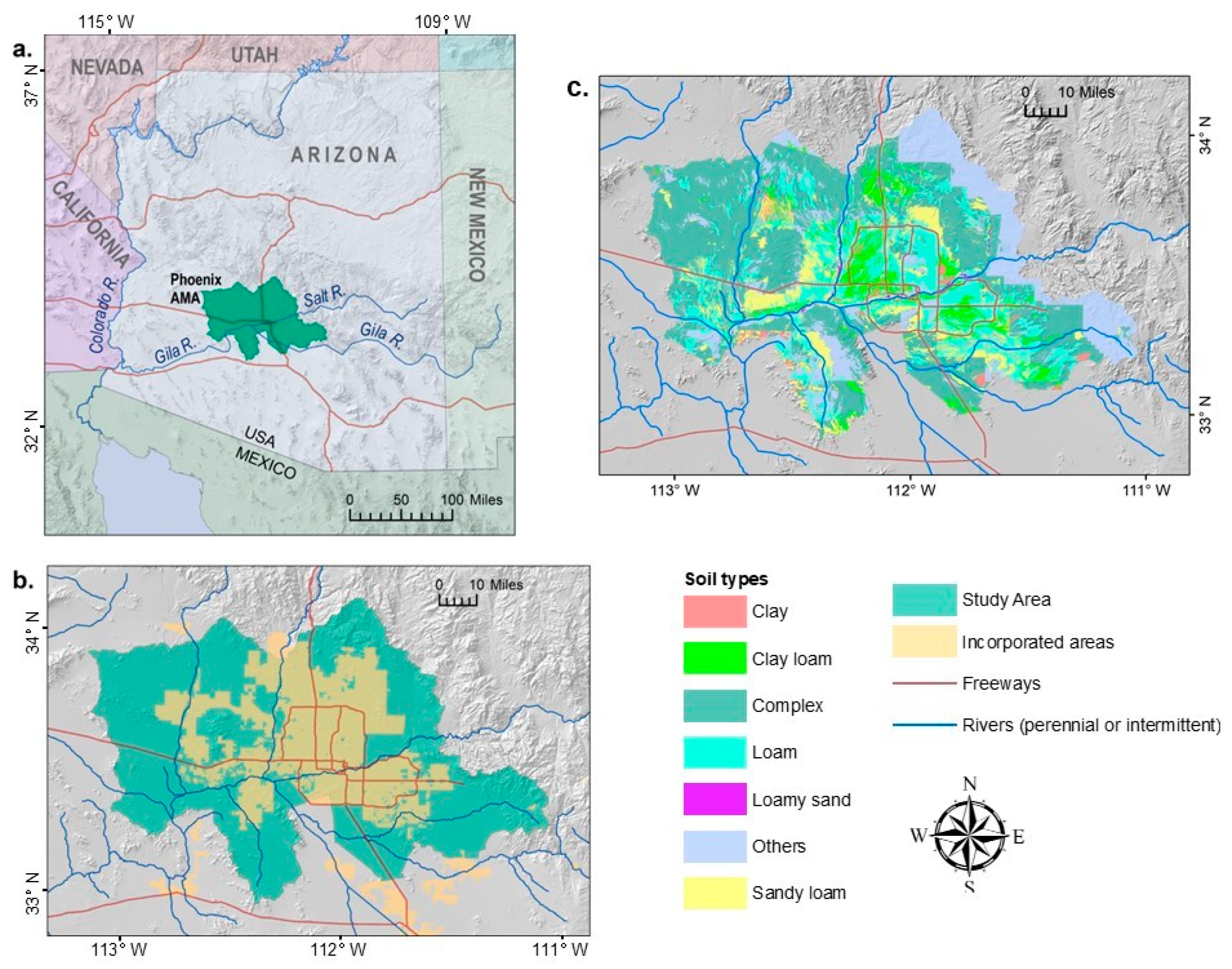
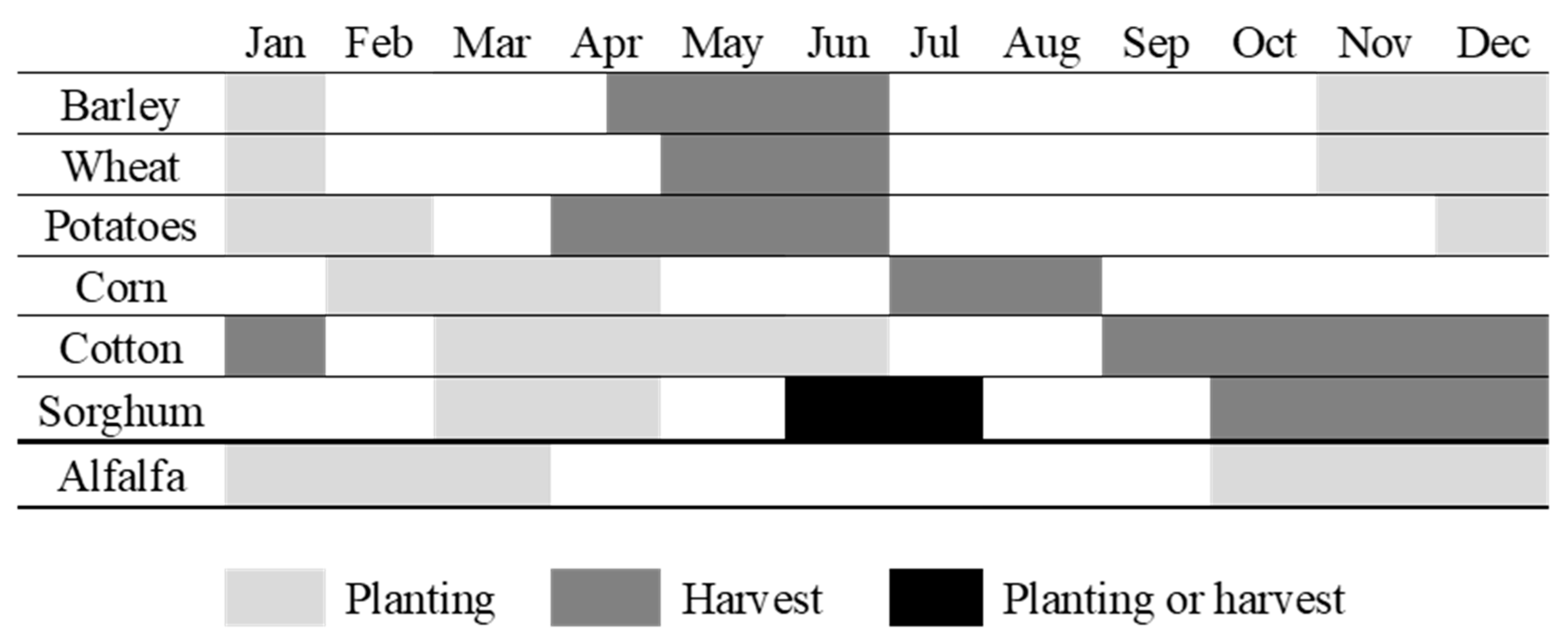
2. Study Area
3. Materials and Methods
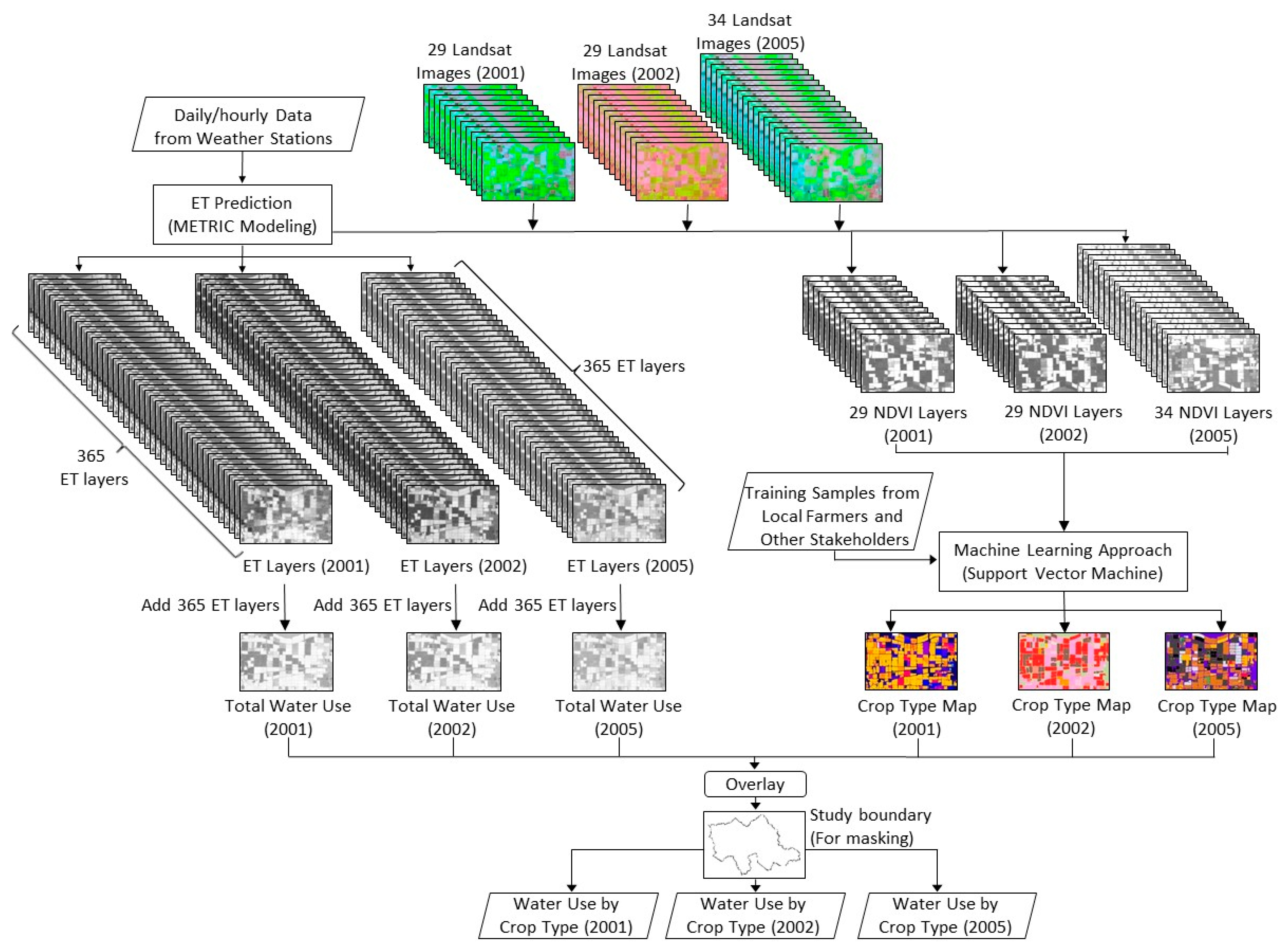
3.1. Prediction of ET
3.2. Annual ET and Water Use Data
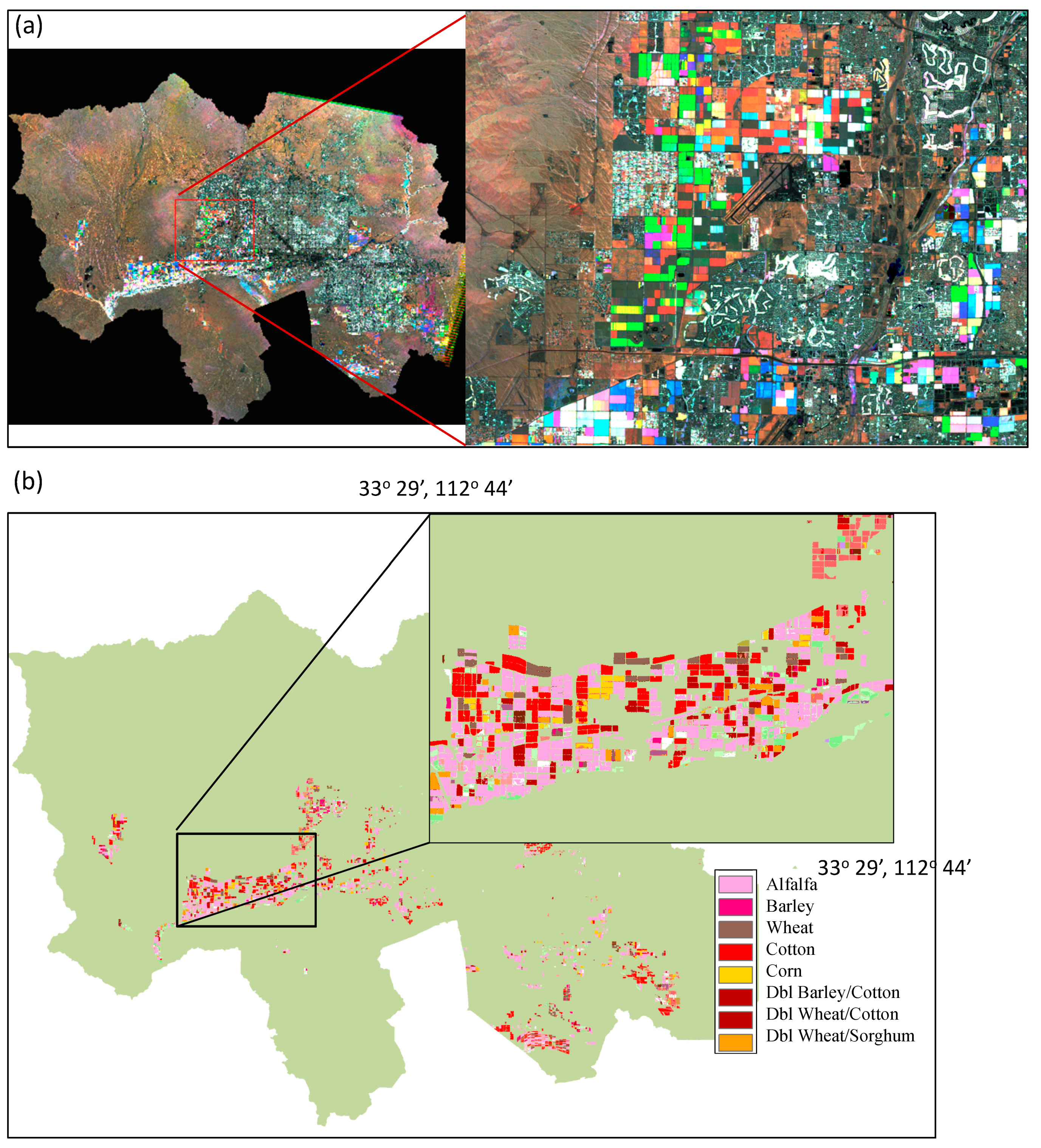
3.3. Crop Type Mapping
3.4. Spatial Data Processing
4. Results and Discussion
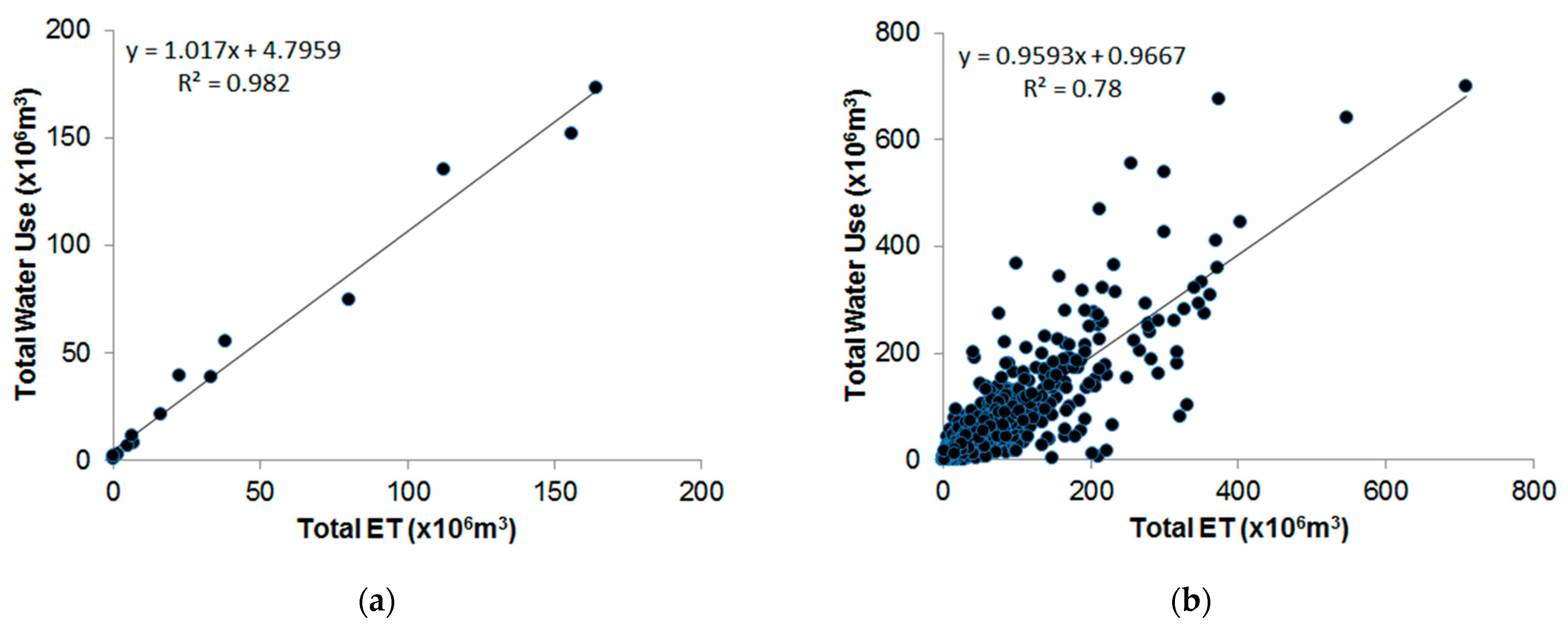
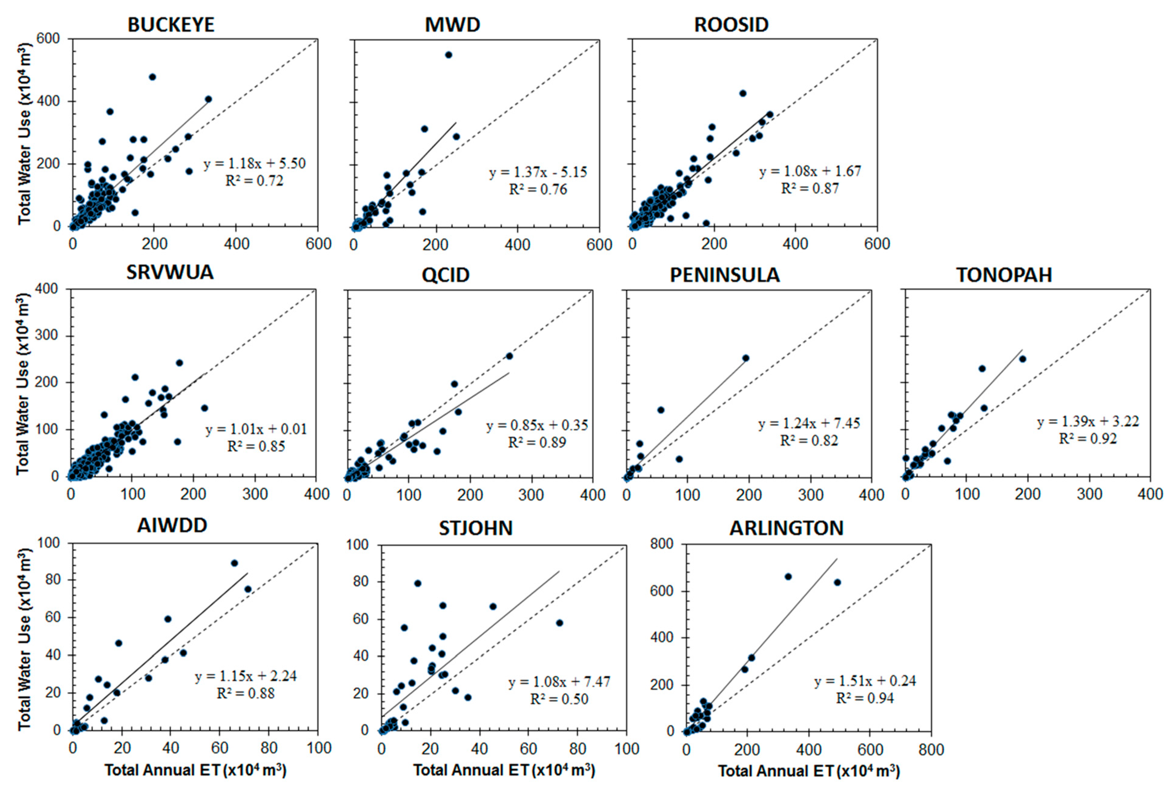
4.1. Relationships between Estimated ET and Water Use Data
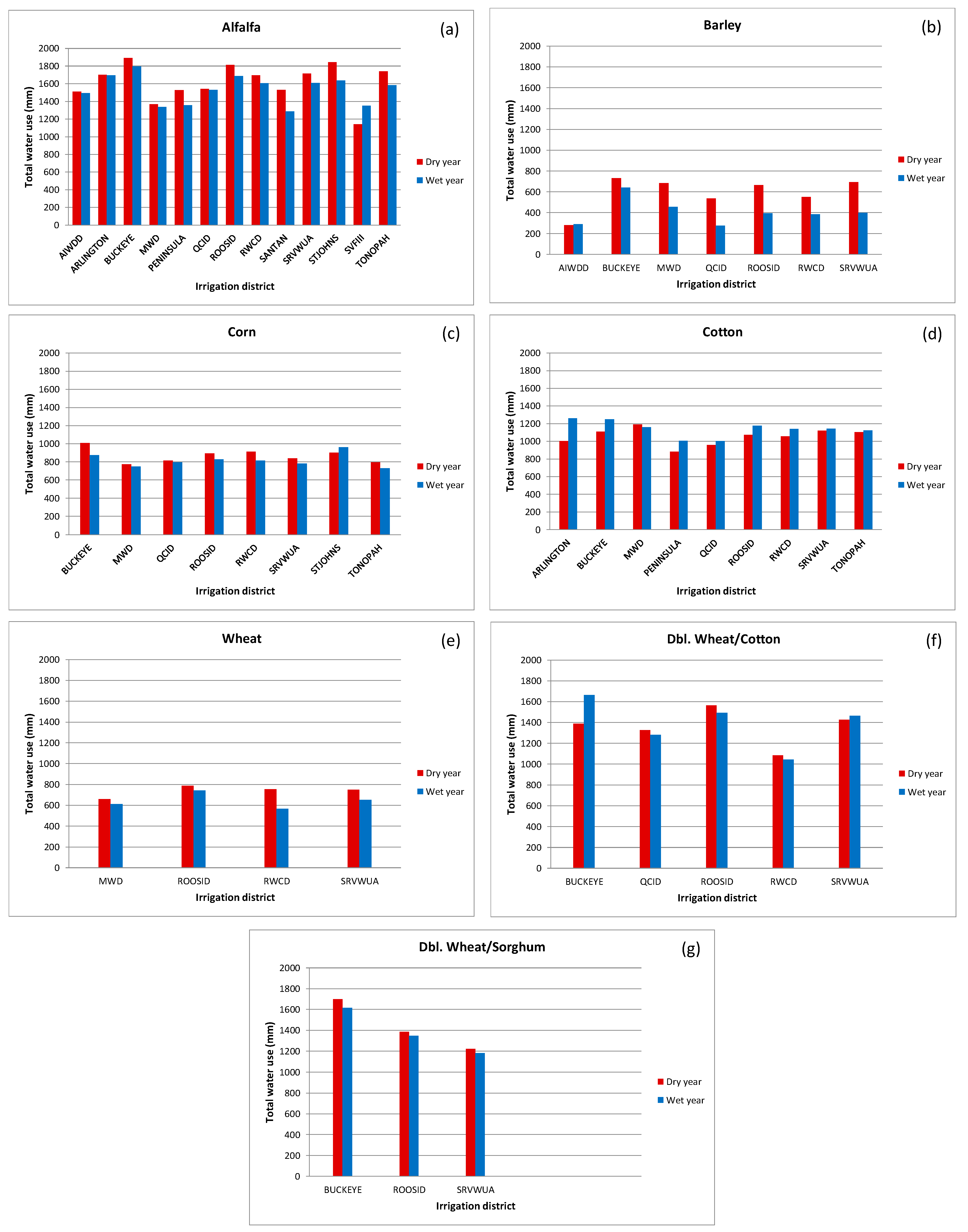
4.2. Variation of Water Consumed across Crops
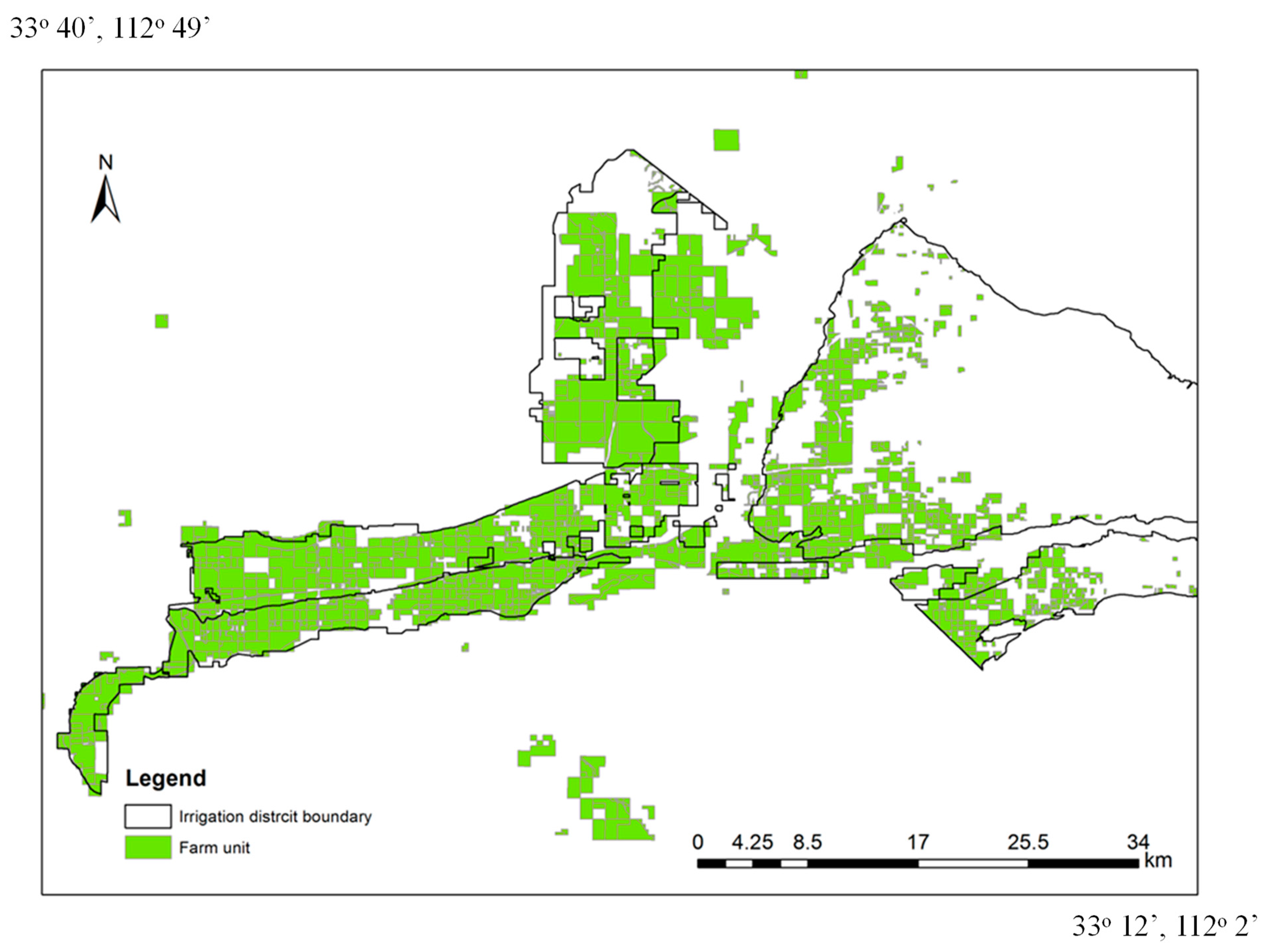
4.3. Variation across Irrigation Districts
4.4. Potential for Water Savings through Appropriate Choice of Crops and Farming Practices
4.5. Comparing Water Consumption under Actual Versus Alternative Cropping Patterns
4.6. Actual Cropping Patterns and Corresponding Water Consumption during Study Period
4.7. Water Saving Potential of Alternative Cropping Patterns: Replacing Alfalfa and Cotton with Wheat and Barley
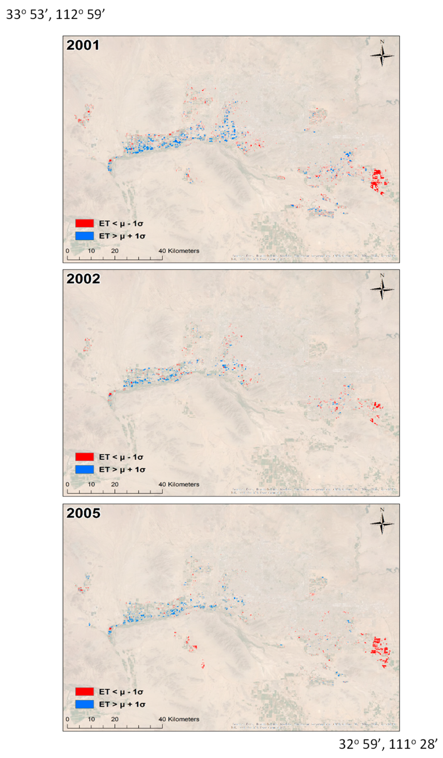
4.8. Identification of Excessive Water Consumption and Considerably Low Water Consumption Areas
5. Conclusions
Author Contributions
Funding
Data Availability Statement
Acknowledgments
Conflicts of Interest
References
- Easterling, D.R.; Kunkel, K.E.; Arnold, J.R.; Knutson, T.; LeGrande, A.N.; Leung, L.R.; Vose, R.S.; Waliser, D.E.; Wehner, M.F. Precipitation Changes in the United States. In Climate Science Special Report: Fourth National Climate Assessment (NCA4); Wuebbles, D.J., Fahey, D.W., Hibbard, K.A., Dokken, D.J., Stewart, B.C., Maycock, T.K., Eds.; Global Change Research Program: Washington, DC, USA, 2017; Volume I, pp. 207–230. [Google Scholar]
- Christensen, J.H.; Hewitson, B.; Busuioc, A.; Chen, A.; Gao, X.; Held, I.; Jones, R.; Kolli, R.K.; Kwon, W.T.; Laprise, R.; et al. Regional Climate Projections. In Climate Change, 2007: The Physical Science Basis. Contribution of Working Group I to the Fourth Assessment Report of the Intergovernmental Panel on Climate Change; Solomon, S., Qin, D., Manning, M., Chen, Z., Marquis, M., Averyt, K.B., Tignor, M., Miller, H.L., Eds.; Cambridge University Press: Cambridge, UK; New York, NY, USA, 2007; pp. 847–940. [Google Scholar]
- Barnett, T.P.; Pierce, D.W.; Hidalgo, H.G.; Bonfils, C.; Santer, B.D.; Das, T.; Bala, G.; Wood, A.W.; Nozawa, T.; Mirin, A.A.; et al. Human-induced changes in the hydrology of the western United States. Science 2008, 319, 1080–1083. [Google Scholar] [CrossRef] [PubMed] [Green Version]
- Rauscher, S.A.; Pal, J.S.; Diffenbaugh, N.S.; Benedetti, M.M. Future changes in snowmelt-driven runoff timing over the western United States. Geophys. Res. Lett. 2008, 35, L16703. [Google Scholar] [CrossRef] [Green Version]
- Karl, T.R.; Melillo, J.M.; Peterson, T.C. Global Climate Change Impacts in the United States; Cambridge University Press: New York, NY, USA, 2009. [Google Scholar]
- Woodhouse, C.A.; Gray, S.T.; Meko, D.M. Updated streamflow reconstructions for the upper Colorado River basin. Water Resour. Res. 2006, 42, W05415. [Google Scholar] [CrossRef]
- Meko, D.M.; Woodhouse, C.A.; Basisan, C.A.; Knight, T.; Lukas, J.J.; Hughes, M.K.; Salzer, M.W. Medieval drought in the upper Colorado River basin. Geophys. Res. Lett. 2007, 34, L10705. [Google Scholar] [CrossRef] [Green Version]
- Bonfils, C.; Santer, B.D.; Pierce, D.W.; Hidalgo, H.G.; Bala, G.; Das, T.; Barnett, T.P.; Cayan, D.R.; Doutriaux, C.; Wood, A.W.; et al. Detection and attribution of temperature changes in the mountainous western United States. J. Clim. 2008, 21, 6404–6424. [Google Scholar] [CrossRef]
- U.S. Department of Agriculture (USDA). Regional Conservation Partnership Program, Colorado River Basin; Natural Resources Conservation Service, USDA: Washington, DC, USA, 2014. Available online: https://www.nrcs.usda.gov/wps/portal/nrcs/detailfull/co/programs/farmbill/rcpp/?cid=nrcseprd1316414 (accessed on 8 April 2021).
- Lapola, D.M.; Oyama, M.D.; Nobre, C.A. Exploring the range of climate biome projections for tropical South America: The role of CO2 fertilization and seasonality. Glob. Biogeochem. Cycles 2009, 23, GB3003. [Google Scholar] [CrossRef]
- Stahlschmidt, Z.R.; DeNardo, D.F.; Holland, J.N.; Kotler, B.P.; Kruse-Peeples, M. Tolerance mechanisms in North American deserts: Biological and societal approaches to climate change. J. Arid. Environ. 2011, 75, 681–687. [Google Scholar] [CrossRef]
- Holmgren, M.; Stapp, P.; Dickman, C.R.; Gracia, C.; Graham, S.; Gutierrez, J.R.; Hice, C.; Jaksic, F.; Kelt, D.A.; Letnic, M.; et al. Extreme climatic events shape arid and semiarid ecosystems. Front. Ecol. Environ. 2006, 4, 87–95. [Google Scholar] [CrossRef] [Green Version]
- Vörösmarty, C.J.; Green, P.; Salisbury, J.; Lammers, R.B. Global water resources: Vulnerability from climate change and population growth. Science 2000, 289, 284–288. [Google Scholar] [CrossRef] [Green Version]
- Malmqvist, B.; Rundle, S.D.; Covich, A.P.; Hildrew, A.G.; Robinson, C.T.; Townsend, C.R. Prospects for streams and rivers: An ecological perspective. In Aquatic Ecosystems: Trends and Global Prospects; Polunin, N.V.C., Ed.; Cambridge University Press: Cambridge, UK, 2008; pp. 19–29. [Google Scholar]
- Dise, N.B. Peatland response to global change. Science 2009, 326, 810–811. [Google Scholar] [CrossRef] [PubMed]
- Smith, R.G.; Knight, R.; Chen, J.; Reeves, J.A.; Zebker, H.A.; Farr, T.; Liu, Z. Estimating the permanent loss of groundwater storage in the southern San Joaquin Valley, California. Water Resour. Res. 2017, 53, 2133–2148. [Google Scholar] [CrossRef]
- Garfin, G.; Franco, G.; Blanco, H.; Comrie, A.; Gonzalez, P.; Piechota, T.; Smyth, R.; Waskom, R. Ch. 20: Southwest. In Climate Change Impacts in the United States: The Third National Climate Assessment; Melillo, J.M., Richmond, T.T.C., Yohe, G.W., Eds.; U.S. Global Change Research Program: Washington, DC, USA, 2014; pp. 462–486. [Google Scholar]
- U.S. Department of Agriculture (USDA). Farm and Ranch Irrigation Survey (2008). In 2007 Census of Agriculture; Special Studies, Part 1.; U.S. Department of Agriculture: Washington, DC, USA, 2008; Volume 3. [Google Scholar]
- Kenny, J.F.; Barber, N.L.; Hutson, S.S.; Linsey, K.S.; Lovelace, J.K.; Maupin, M.A. Estimated Use of Water in the United States in 2005. U.S. Geol. Surv. Circ. 2009, 1344, 52. [Google Scholar]
- Amarasinghe, U.A.; Smakhtin, V.U. Global water demand projections: Past, present and future. In IWMI Research Report 156; International Water Management Institute (IWMI): Colombo, Sri Lanka, 2014. [Google Scholar]
- Flörke, M.; Schneider, C.; McDonald, R. Water competition between cities and agriculture driven by climate change and urban growth. Nat. Sustain. 2018, 1, 51–58. [Google Scholar] [CrossRef]
- Lundquist, J.D.; Loheide II, S.P. How evaporative water losses vary between wet and dry water years as a function of elevation in the Sierra Nevada, California, and critical factors for modeling. Water Resour. Res. 2011, 47, W00H09. [Google Scholar] [CrossRef] [Green Version]
- Goldstein, A.H.; Hultman, N.E.; Fracheboud, J.M.; Bauer, M.R.; Panek, J.A.; Xu, M.; Qi, Y.; Guenther, A.B.; Baugh, W. Effects of climate variability on the carbon dioxide, water, and sensible heat fluxes above a ponderosa pine plantation in the Sierra Nevada (CA). Agric. For. Meteorol. 2000, 101, 113–129. [Google Scholar] [CrossRef] [Green Version]
- Hamlet, A.F.; Mote, P.W.; Clark, M.P.; Lettenmaier, D.P. Twentieth-century trends in runoff, evapotranspiration, and soil moisture in the Western United States. J. Clim. 2007, 20, 1468–1485. [Google Scholar] [CrossRef] [Green Version]
- Arizona Department of Water Resources (ADWR). Arizona Water Atlas—Volume 8—Active Management Area Planning Area; 2010. Available online: https://www.resolutionmineeis.us/sites/default/files/references/adwr-arizona-water-atlas-vol-8-2010.pdf (accessed on 8 April 2021).
- U.S. Department of Agriculture (USDA)—Natural Resources Conservation Service (NRCS). Land Resource Regions and Major Land Resource Areas of the United States, the Caribbean, and the Pacific Basin (USDA Handbook 296); 2006. Available online: https://www.nrcs.usda.gov/Internet/FSE_DOCUMENTS/nrcs142p2_051845.pdf (accessed on 21 March 2021).
- Hendrickx, J.M.H.; Hong, S.H. Mapping sensible and latent heat fluxes in arid areas using optical imagery. Proc. Int. Soc. Opt. Eng. SPIE 2005, 5811, 138–146. [Google Scholar]
- Kaplan, S.; Myint, S.W. Estimating agricultural water use through Landsat TM and a simplified surface energy balance modeling in the semi-arid environments of Arizona. Photogramm. Eng. Remote. Sens. 2012, 78, 849–859. [Google Scholar] [CrossRef]
- Wang, C.; Turner, V.K.; Wentz, E.A.; Zhao, Q.; Myint, S.W. Optimization of residential green space for environmental sustainability and property appreciation in metropolitan Phoenix, Arizona. Sci. Total Environ. 2021, 763, 144605. [Google Scholar] [CrossRef] [PubMed]
- Allen, R.G.; Tasumi, M.; Morse, A.; Trezza, R.; Kramber, W.; Lorite, I. Satellite-based energy balance for mapping evapotranspiration with internalized calibration (METRIC)—Applications. J. Irrig. Drain. Eng. 2007, 133, 395–406. [Google Scholar] [CrossRef]
- Bastiaanssen, W.G.M.; Ahmad, M.D.; Chemin, Y. Satellite surveillance of evaporative depletion across the Indus Basin. Water Resour. Res. 2002, 38, 1273. [Google Scholar] [CrossRef]
- Hong, S.H.; Hendrickx, J.M.H.; Borchers, B. Effect of scaling transfer between evapotranspiration maps derived from LandSat 7 and MODIS images. Proc. Int. Soc. Opt. Eng. SPIE 2005, 5811, 147–158. [Google Scholar]
- Hafeez, M.; Andreini, M.; Liebe, J.; Friesen, J.; Marx, A.; Giesen, N.V.D. Hydrological parameterization through remote sensing in Volta Basin, West Africa. Int. J. River Basin Manag. 2006, 4, 1–8. [Google Scholar] [CrossRef]
- Hong, S.H.; Hendrickx, J.M.H.; Borchers, B. Up-scaling of SEBAL derived evapotranspiration maps from Landsat (30 m) to MODIS (250 m) scale. J. Hydrol. 2009, 370, 122–138. [Google Scholar] [CrossRef]
- Hong, S.H.; Hendrickx, J.M.H.; Borchers, B. Downscaling of SEBAL derived evapotranspiration map from MODIS (250 m) to Landsat (30 m) scale. Int. J. Remote Sens. 2011, 32, 6457–6477. [Google Scholar] [CrossRef]
- Allen, R.G.A.; Irmak, A.; Trezza, R.; Hendrickx, J.M.H.; Bastiaanssen, W.G.M.; Kjaersgaard, J. Satellite-based ET estimation in agriculture using SEBAL and METRIC. Hydrol. Process. 2011, 25, 4011–4027. [Google Scholar] [CrossRef]
- Hendrickx, J.M.H.; Allen, R.G.; Brower, A.; Byrd, A.R.; Hong, S.H.; Ogden, F.L.; Pradhan, N.R.; Robison, C.W.; Toll, D.; Trezza, R.; et al. Benchmarking optical/thermal satellite imagery for estimating evapotranspiration and soil moisture in decision support tools. J. Am. Water Resour. Assoc. 2016, 52, 89–119. [Google Scholar] [CrossRef]
- Bastiaanssen, W.G.M.; Menenti, M.; Feddes, R.A.; Holtslag, A.A.M. A remote sensing surface energy balance algorithm for land (SEBAL): 1. Formulation. J. Hydrol. 1998, 212, 198–212. [Google Scholar] [CrossRef]
- Allen, R.G.; Burnett, B.; Kramber, W.; Huntington, J.; Kjaersgaard, J.; Kilic, A.; Kelly, C.; Trezza, R. Automated calibration of the METRIC-Landsat evapotranspiration process. J. Am. Water Resour. Assoc. 2013, 49, 563–576. [Google Scholar] [CrossRef]
- Bastiaanssen, W.G.W.; Noordman, E.J.M.; Pelgrum, H.; Davids, G.; Thoreson, B.P.; Allen, R.G. SEBAL model with remotely sensed data to improve water-resources management under actual field conditions. J. Irrig. Drain. Eng. 2005, 131, 85–93. [Google Scholar] [CrossRef]
- Allen, R.G.; Tasumi, M.; Trezza, R. Satellite-based Energy Balance for Mapping Evapotranspiration with Internalized Calibration (METRIC)—Model. J. Irrig. Drain. Eng. 2007, 133, 380–394. [Google Scholar] [CrossRef]
- Trezza, R. Evapotranspiration Using a Satellite-Based Surface Energy Balance with Standardized Ground Control. Ph.D. Dissertation, Utah State University, Logan, UT, USA, 2002. [Google Scholar]
- Allen, R.G.; Walter, I.A.; Elliott, R.; Howell, T.; Itenfisu, D.; Jensen, M. The ASCE Standardized Reference Evapotranspiration Equation; 2005. Available online: https://xwww.mesonet.org/images/site/ASCE_Evapotranspiration_Formula.pdf (accessed on 8 April 2021).
- Zheng, B.; Myint, S.W.; Thenkabail, P.S.; Aggarwal, R. A support vector machine to identify irrigated crop types using time-series Landsat NDVI data. Int. J. Appl. Earth Obs. Geoinf. 2015, 34, 103–112. [Google Scholar] [CrossRef]
- Foody, G.M.; Mathur, A. Toward intelligent training of supervised image classifications: Directing training data acquisition for SVM classification. Remote Sens. Environ. 2004, 93, 107–117. [Google Scholar] [CrossRef]
- Plaza, A.; Benediktsson, J.A.; Boardman, J.W.; Brazile, J.; Bruzzone, L.; Camps-Valls, G.; Chanussot, J.; Fauvel, M.; Gamba, P.; Gualtieri, A.; et al. Recent advances in techniques for hyperspectral image processing. Remote Sens. Environ. 2009, 113, S110–S122. [Google Scholar] [CrossRef]
- Shao, Y.; Lunetta, R.S. Comparison of support vector machine, neural network, and CART algorithms for the land-cover classification using limited training data points. ISPRS J. Photogramm. Remote Sens. 2012, 70, 78–87. [Google Scholar] [CrossRef]
- Congalton, R.; Green, K. Assessing the Accuracy of Remotely Sensed Data: Principles and Practices, 2nd ed.; CRC Press: Boca Raton, FL, USA, 2008. [Google Scholar]
- Morse, A.; Kramber, W.J.; Allen, R. Cost comparison for monitoring irrigation water use: Landsat thermal data versus power consumption data. In Proceedings of the Pecora 17—The Future of Land Imaging Going Operational. Annual Meeting of the American Society of Photogrammetry and Remote Sensing, Denver, CO, USA, 18–20 November 2008. [Google Scholar]
- Wang, H.; Zhang, L.; Dawes, W.R.; Liu, C. Improving water use efficiency of irrigated crops in the North China Plain—Measurements and modelling. Agric. Water Manag. 2001, 48, 151–167. [Google Scholar] [CrossRef]
- U.S. Department of Agriculture (USDA)—National Agricultural Statistics Service (NASS). 2004 Arizona Agricultural Statistics Bulletin; 2004. Available online: https://www.nass.usda.gov/Statistics_by_State/Arizona/Publications/Annual_Statistical_Bulletin/historical_bulletins/2004FullBulletin.pdf (accessed on 21 March 2021).
- Fleck, B.E. Factors Affecting Agricultural Water Use and Sourcing in Irrigation Districts of Central Arizona. Master’s Thesis, University of Arizona, Tucson, Arizona, 2013. [Google Scholar]
- Hunt, P.G.; Bauer, P.J.; Matheny, T.A. Crop production in a wheat-cotton doublecrop rotation with conservation tillage. J. Prod. Agric. 1997, 10, 462–465. [Google Scholar] [CrossRef]
- Zhang, Y.; Kendy, E.; Qiang, Y.; Changming, L.; Yanjun, S. Effect of soil water deficit on evapotranspiration, crop yield, and water use efficiency in the North China Plain. Agric. Water Manag. 2004, 64, 107–122. [Google Scholar] [CrossRef]
- Foulia, Y.; Duikerb, S.W.; Fritton, D.D.; Hallb, M.H.; Watsond, J.E.; Johnsone, D.H. Double cropping effects on forage yield and the field water balance. Agric. Water Manag. 2012, 115, 104–117. [Google Scholar] [CrossRef]
- Unger, P.W.; Vigil, M.F. Cover crop effects on soil water relationships. J. Soil Water Conserv. 1998, 53, 200–207. [Google Scholar]
- Gregory, M.M.; Shea, K.L.; Bakko, E.B. Comparing agroecosystems: Effects of cropping and tillage patterns on soil, water, energy use and productivity. Renew. Agric. Food Syst. 2005, 20, 81–90. [Google Scholar] [CrossRef]
- Joyce, B.A.; Wallender, W.W.; Mitchell, J.P.; Huyck, L.M.; Temple, S.R.; Brostrom, P.N.; Hsiao, T.C. Infiltration and soil water storage under winter cover cropping in California’s Sacramento Valley. Trans. Am. Soc. Agric. Eng. 2002, 45, 315–326. [Google Scholar] [CrossRef]
- Blake, C. Minimum Tillage Spells Success for Arizona’s Ron Rayner; Western Farm Press: Fresno, CA, USA, 2018. [Google Scholar]
- Frisvold, B.F. Developing Sustainability Metrics for Water Use in Arizona Small Grain Production; Final Report to the Arizona Grain Research and Promotion Council: Tucson, AZ, USA, 2015; p. 20. [Google Scholar]
- Intergovernmental Panel on Climate Change (IPCC). Climate Change 2014: Synthesis Report; 2014. Available online: https://reliefweb.int/sites/reliefweb.int/files/resources/SYR_AR5_FINAL_full.pdf (accessed on 21 March 2021).
- Olesen, J.E.; Trnka, M.; Kersebaum, K.; Skjelvåg, A.; Seguin, B.; Peltonen-Sainio, P.; Rossi, F.; Kozyra, J.; Micale, F. Impacts and adaptation of European crop production systems to climate change. Eur. J. Agron. 2011, 34, 96–112. [Google Scholar] [CrossRef]
- Lobell, D.B.; Hammer, G.L.; McLean, G.; Messina, C.; Roberts, M.J.; Schlenker, W. The critical role of extreme heat for maize production in the United States. Nat. Clim. Chang. 2013, 3, 497–501. [Google Scholar] [CrossRef]
- Porter, J.R.; Xie, L.; Challinor, A.J.; Cochrane, K.; Howden, S.M.; Iqbal, M.M.; Lobell, D.B.; Travasso, M.I. Chapter 7: Food Security and Food Production Systems. In Climate Change 2014: Impacts, Adaptation, and Vulnerability. Part. A: Global and Sectoral Aspects. Contribution of Working Group II to the Fifth Assessment Report of the Intergovernmental Panel on Climate Change; Field, C.B., Barros, V., Dokken, D., Mach, K., Mastrandrea, M., Bilir, T., Chatterjee, M., Ebi, K., Estrada, Y., Genova, R., et al., Eds.; Cambridge University Press: Cambridge, UK; New York, NY, USA, 2014; pp. 485–533. [Google Scholar]
- Edenhofer, O.; Pichs-Madruga, R.; Sokona, Y.; Minx, J.; Farahani, E.; Kadner, S.; Seyboth, K.; Adler, A.; Baum, I.; Baum, S.; et al. Technical Summary. In Climate Change 2014: Mitigation of Climate Change. Contribution of Working Group III to the Fifth Assessment Report of the Intergov-ernmental Panel on Climate Change; Edenhofer, O., Pichs-Madruga, R., Sokona, Y., Minx, J., Farahani, E., Kadner, S., Seyboth, K., Adler, A., Baum, I., Baum, S., et al., Eds.; Cambridge University Press: Cambridge, UK; New York, NY, USA, 2014; pp. 33–110. [Google Scholar]


| Reference | ||||||||||||
|---|---|---|---|---|---|---|---|---|---|---|---|---|
| Classified | Alf | Cot | Cor | Whe | Alf-Cot | Cor-Alf | Whe-Sor | Whe-Cot | O-Crops | Total | Pro-Accu | Usr-Accu |
| Alf | 114 | 0 | 0 | 0 | 0 | 0 | 0 | 0 | 6 | 120 | 95 | 95 |
| Cot | 0 | 109 | 0 | 0 | 0 | 0 | 0 | 0 | 1 | 110 | 100 | 99 |
| Cor | 0 | 0 | 32 | 0 | 0 | 0 | 0 | 0 | 7 | 39 | 94 | 82 |
| Whe | 1 | 0 | 2 | 42 | 0 | 0 | 2 | 0 | 2 | 49 | 100 | 86 |
| Alf-Cot | 1 | 0 | 0 | 0 | 25 | 0 | 0 | 0 | 4 | 30 | 100 | 83 |
| Cor-Alf | 0 | 0 | 0 | 0 | 0 | 28 | 0 | 0 | 2 | 30 | 100 | 93 |
| Whe-Sor | 1 | 0 | 0 | 0 | 0 | 0 | 27 | 0 | 2 | 30 | 84 | 90 |
| Whe-Cot | 0 | 0 | 0 | 0 | 0 | 0 | 3 | 26 | 3 | 32 | 100 | 81 |
| O-crops | 3 | 0 | 0 | 0 | 0 | 0 | 0 | 0 | 80 | 83 | 75 | 96 |
| Total | 120 | 109 | 34 | 42 | 25 | 28 | 32 | 26 | 107 | 523 | ||
| Mean Water Use | Mean Water Use | Water Use | ||
|---|---|---|---|---|
| (Dry Year) | (Wet Year) | Difference | (Mean Dry and Wet Year) | |
| (mm) | (mm) | (mm) | (mm) | |
| Alfalfa | 1616.16 | 1536.05 | 80.11 | 1576.11 |
| Barley | 591.56 | 405.56 | 186.00 | 498.56 |
| Corn | 867.41 | 817.79 | 49.62 | 842.60 |
| Cotton | 1054.80 | 1139.04 | −84.24 | 1096.92 |
| Wheat | 737.75 | 643.75 | 94.00 | 690.75 |
| Dbl. Wheat/Cotton | 1357.89 | 1388.90 | −31.01 | 1373.39 |
| Dbl. Wheat/Sorghum | 1435.00 | 1381.28 | 53.72 | 1408.14 |
| Crop Type | USDA (All of Arizona) (mm) | Our Study (Maricopa County) (mm) | Difference: USDA and This Study | ||
|---|---|---|---|---|---|
| Average | Wet | Dry | |||
| Alfalfa | 1889.76 | 1575.82 | 1536.19 | 1615.44 | 313.94 |
| Cotton | 1463.04 | 1097.28 | 1139.95 | 1054.61 | 365.76 |
| Wheat | 1097.28 | 664.46 | 609.60 | 722.38 | 432.82 |
| Corn | 1097.28 | 853.44 | 829.06 | 874.78 | 243.84 |
| Number of Observations = 98 Root MSE = 101.781 | R-Squared = 0.9530 Adjusted R-Squared = 0.9415 | ||||
|---|---|---|---|---|---|
| Source | Partial SS | df | MS | F | Prob > F |
| Model | 16,382,967.60 | 19 | 862,261.45 | 83.24 | 0.0000 |
| Crop type | 13,644,609.80 | 6 | 2,274,101.64 | 219.52 | 0.0000 |
| Irrigation District | 1,058,549.38 | 12 | 88,212.45 | 8.52 | 0.0000 |
| Year | 108,394.45 | 1 | 108,394.45 | 10.46 | 0.0018 |
| Residual | 808,028.94 | 78 | 359.35 | ||
| Total | 17,190,996.50 | 97 | 177,226.77 |
| Barley | Cotton | Barley & Cotton | Double Cropping | ||
|---|---|---|---|---|---|
| as Single Crops | Barley/Cotton | ||||
| Water Use (liter/m2) | 746 | 1090 | 1837 | 1417 | Water Saving |
| Crop area (m2) | 9,763,209 | 78,086,769 | 87,849,978 | 9,223,208 | Double cropping |
| Water use (Million Liters) | 7288 | 85,142 | 161,365 | 124,459 | Barley & Cotton |
| Water Saving by growing double cropping Barley/Cotton (liter/m2) | 420 | ||||
| Water saving by growing double cropping Barley/Cotton (%) | 22.87% | ||||
| Water Saving (million liter) using total area (87,849,978 m2) of Barley & Cotton as single crops | 36,906 | ||||
| Liter per m2 | Average Liter per m2 | Litre/m2 Difference between Dry and Wet | Increase or Decrease (%) | Total Area (m2) | Total Water Consumed (Million Liters) | Difference between Dry and Wet (Million Liters) | Average Water Consumed per Year (Million Liters) | Water Consumed by Crop Type (%) | |
|---|---|---|---|---|---|---|---|---|---|
| Al (Dry) | 1616 | 1576 | 80 | 5.22 | 124,706,810 | 201,546 | 20,281 | 191,406 | 56.81% |
| Al (Wet) | 1536 | 118,007,204 | 181,265 | ||||||
| Br (Dry) | 592 | 499 | 186 | 45.86 | 9,763,209 | 5776 | 5016 | 3268 | 0.97% |
| Br (Wet) | 406 | 1,873,802 | 760 | ||||||
| Cn (Dry) | 867 | 843 | 50 | 6.07 | 29,567,726 | 25,647 | –2646 | 26,971 | 8.01% |
| Cn (Wet) | 818 | 34,597,831 | 28,294 | ||||||
| Ct (Dry) | 1055 | 1097 | −84 | −7.40 | 78,086,769 | 82,366 | –6143 | 85,438 | 25.36% |
| Ct (Wet) | 1139 | 77,705,169 | 88,509 | ||||||
| Wh (Dry) | 738 | 691 | 94 | 14.60 | 6,374,706 | 4703 | –13,135 | 11,271 | 3.35% |
| Wh (Wet) | 644 | 27,710,124 | 17,838 | ||||||
| Wh/Ct (Dry) | 1358 | 1373 | −31 | −2.23 | 9,223,208 | 12,524 | 8890 | 8079 | 2.40% |
| Wh/Ct (Wet) | 1389 | 2,616,302 | 3634 | ||||||
| Wh/So (Dry) | 1435 | 1408 | 54 | 3.89 | 3,411,003 | 4895 | –11,183 | 10,486 | 3.11% |
| Wh/So (Wet) | 1381 | 11,639,710 | 16,078 |
| More Water | ||||
|---|---|---|---|---|
| Crop Type | Water | Dry Year | Water | Consumed |
| per Year | Consumed | Area | Consumed | in Dry Year |
| (Liter/m2) | (m2) | (Million Liters) | (Million Liters) | |
| Al (Dry) | 1616 | 124,706,810 | 201,546 | 9990 |
| Al (Wet) | 1536 | 124,706,810 | 191,556 | |
| Br (Dry) | 592 | 9,763,209 | 5776 | 1816 |
| Br (Wet) | 406 | 9,763,209 | 3960 | |
| Cn (Dry) | 867 | 29,567,726 | 25,647 | 1467 |
| Cn (Wet) | 818 | 29,567,726 | 24,180 | |
| Wh (Dry) | 738 | 6,374,706 | 4703 | 599 |
| Wh (Wet) | 644 | 6,374,706 | 4104 | |
| Wh/So (Dry) | 1435 | 3,411,003 | 4895 | 183 |
| Wh/So (Wet) | 1381 | 3,411,003 | 4712 |
| Same Area | More Water | |||
|---|---|---|---|---|
| Crop Type | Water | for | Water | Consumed |
| per Year | Consumed | All Crops | Consumed | in Dry Year |
| (Liter/m2) | (m2) | (Million Liters) | (Million Liters) | |
| Al (Dry) | 1616 | 34,764,691 | 56,185 | 2785 |
| Al (Wet) | 1536 | 34,764,691 | 53,400 | |
| Br (Dry) | 592 | 34,764,691 | 20,565 | 6466 |
| Br (Wet) | 406 | 34,764,691 | 14,099 | |
| Cn (Dry) | 867 | 34,764,691 | 30,155 | 1725 |
| Cn (Wet) | 818 | 34,764,691 | 28,430 | |
| Wh (Dry) | 738 | 34,764,691 | 25,648 | 3268 |
| Wh (Wet) | 644 | 34,764,691 | 22,380 | |
| Wh/So (Dry) | 1435 | 34,764,691 | 49,887 | 1868 |
| Wh/So (Wet) | 1381 | 34,764,691 | 48,020 |
| 2001 | 2002 | 2005 | Total | Average/yr | % Crop Area | |
|---|---|---|---|---|---|---|
| (m2) | (m2) | (m2) | (m2) | (m2) | ||
| Alfalfa | 153,182,835 | 124,706,810 | 118,007,204 | 395,896,850 | 131,965,617 | 42.55% |
| Barley | - | 9,763,209 | 1,873,802 | 11,637,010 | 5,818,505 | 1.88% |
| Cotton | 121,825,908 | 78,086,769 | 77,705,169 | 277,617,845 | 92,539,282 | 29.84% |
| Corn | 34,850,731 | 29,567,726 | 34,597,831 | 99,016,288 | 33,005,429 | 10.64% |
| Wheat | 41,835,637 | 6,374,706 | 27,710,124 | 75,920,467 | 25,306,822 | 8.16% |
| Barley/Cotton | - | 9,223,208 | - | 9,223,208 | 9,223,208 | 2.97% |
| Wheat/Cotton | 8,838,908 | 2,301,302 | 2,616,302 | 13,756,512 | 4,585,504 | 1.48% |
| Wheat/Sorghum | 8,082,007 | 3,411,003 | 11,639,710 | 23,132,720 | 7,710,907 | 2.49% |
| Water (Million Liters) 2001 | Water (Million Liters) 2002 | Water (Million Liters) 2005 | Al => Bar Cot => Wh (Million Liters) 2001 | Al => Bar Cot => Wh (Million Liters) 2002 | Al => Bar Cot => Wh (Million Liters) 2005 | Total Saving (Million Liters) 2001 | Total Saving (Million Liters) 2002 | Total Saving (Million Liters) 2005 | |
|---|---|---|---|---|---|---|---|---|---|
| Al | 2414 | 1966 | 1860 | ||||||
| Ct | 1027 | 658 | 655 | ||||||
| Br | - | 49 | 9 | 764 | 670 | 598 | |||
| Wh | 289 | 44 | 191 | 1130 | 583 | 728 | |||
| Total | 3730 | 2716 | 2715 | 1894 | 1254 | 1326 | 1836 | 1462 | 1390 |
| Crop Type | 2001 (ET) | 2002 (ET) | 2005 (ET) |
|---|---|---|---|
| (Std) | (Std) | (Std) | |
| Alfalfa | 371.21 | 294.22 | 377.04 |
| Barley | - | 276.46 | 340.25 |
| Corn | 296.31 | 270.75 | 434.08 |
| Cotton | 356.01 | 314.08 | 438.1 |
| Wheat | 395.49 | 153.19 | 384.59 |
| Wheat/Cotton | 262.09 | 248.29 | 200.47 |
| Wheat/Sorghum | 260.71 | 301.84 | 309.41 |
| Crop Type | 2001 (Over) | 2001 (Stress) | 2002 (Over) | 2002 (Stress) | 2005 (Over) | 2005 (Stress) |
|---|---|---|---|---|---|---|
| Ha (%) | Ha (%) | Ha (%) | Ha (%) | Ha (%) | Ha (%) | |
| Alfalfa | 2785 (18%) | 2447 (16%) | 1488 (12%) | 1507 (12%) | 1182 (10%) | 977 (8%) |
| Barley | - | - | 124 (13%) | 58 (6%) | 55 (29%) | 63 (34%) |
| Corn | 444 (13%) | 138 (4%) | 300 (10%) | 175 (6%) | 402 (12%) | 8.46 (<1%) |
| Cotton | 1453 (12%) | 882 (7%) | 391 (5%) | 189 (2%) | 238 (3%) | 113 (1%) |
| Wheat | 775 (19%) | 243 (6%) | 101 (16%) | 90 (14%) | 654 (24%) | 441 (16%) |
| Wheat/Cotton | 170 (19%) | 162 (18%) | 34 (15%) | 41 (18%) | 35 (13%) | 45 (17%) |
| Wheat/Sorghum | 144 (18%) | 131 (16%) | 77 (22%) | 44 (13%) | 179 (15%) | 136 (12%) |
Publisher’s Note: MDPI stays neutral with regard to jurisdictional claims in published maps and institutional affiliations. |
© 2021 by the authors. Licensee MDPI, Basel, Switzerland. This article is an open access article distributed under the terms and conditions of the Creative Commons Attribution (CC BY) license (https://creativecommons.org/licenses/by/4.0/).
Share and Cite
Myint, S.W.; Aggarwal, R.; Zheng, B.; Wentz, E.A.; Holway, J.; Fan, C.; Selover, N.J.; Wang, C.; Fischer, H.A. Adaptive Crop Management under Climate Uncertainty: Changing the Game for Sustainable Water Use. Atmosphere 2021, 12, 1080. https://doi.org/10.3390/atmos12081080
Myint SW, Aggarwal R, Zheng B, Wentz EA, Holway J, Fan C, Selover NJ, Wang C, Fischer HA. Adaptive Crop Management under Climate Uncertainty: Changing the Game for Sustainable Water Use. Atmosphere. 2021; 12(8):1080. https://doi.org/10.3390/atmos12081080
Chicago/Turabian StyleMyint, Soe W., Rimjhim Aggarwal, Baojuan Zheng, Elizabeth A. Wentz, Jim Holway, Chao Fan, Nancy J. Selover, Chuyuan Wang, and Heather A. Fischer. 2021. "Adaptive Crop Management under Climate Uncertainty: Changing the Game for Sustainable Water Use" Atmosphere 12, no. 8: 1080. https://doi.org/10.3390/atmos12081080