
Central Control for Optimized Herbaceous Feedstock Delivery to a Biorefinery from Satellite Storage Locations


1
Department of Geographical Sciences, University of Maryland, College Park, MD 20740, USA
2
Department of Biological Systems Engineering, Virginia Tech, Blacksburg, VA 24060, USA
*
Author to whom correspondence should be addressed.
AgriEngineering 2022, 4(2), 544-565; https://doi.org/10.3390/agriengineering4020037
Submission received: 24 May 2022
/
Revised: 11 June 2022
/
Accepted: 14 June 2022
/
Published: 17 June 2022
Abstract
:The delivery of herbaceous feedstock from satellite storage locations (SSLs) to a biorefinery or preprocessing depot is a logistics problem that must be optimized before a new bioenergy industry can be realized. Both load-out productivity, defined as the loading of 5 × 4 round bales into a 20-bale rack at the SSL, and truck productivity, defined as the hauling of bales from the SSLs to the biorefinery, must be maximized. Productivity (Mg/d) is maximized and cost (USD/Mg) is minimized when approximately the same number the loads is received each day. To achieve this, a central control model is proposed, where a feedstock manager at the biorefinery can dispatch a truck to any SSL where a load will be available when the truck arrives. Simulations of this central control model for different numbers of simultaneous load-out operations were performed using a database of potential production fields within a 50 km radius of a theoretical biorefinery in Gretna, VA. The minimum delivered cost (i.e., load-out plus truck) was achieved with nine load-outs and a fleet of eight trucks. The estimated cost was 11.24 and 11.62 USD/Mg of annual biorefinery capacity (assuming 24/7 operation over 48 wk/y for a total of approximately 150,000 Mg/y) for the load-out and truck, respectively. The two costs were approximately equal, reinforcing the desirability of a central control to maximize the productivity of these two key operations simultaneously.
1. Introduction
The United States continues to strive for renewable energy sources as a way to reduce its reliance on fossil fuels, which contribute to climate change. The US Department of Energy (DOE) has set a goal of replacing at least 30% of the country’s current petroleum consumption with biomass by 2030 [1]. Towards this endeavor, many studies have demonstrated the potential for different regions of the country to grow sustainable biomass [2,3,4]. These studies generally organize areas into production zones, defined as multicounty regions that have the potential to supply a biorefinery with herbaceous feedstock [4]. However, more research is needed to explore the logistics of delivering the feedstock supply within these production zones to the biorefinery.
In general, the term “biorefinery” refers to any processing plant that converts a biological material into a manufactured product. This study focused on the conversion of herbaceous biomass into an energy product or perhaps coproducts. The simplest example would be the grinding of the raw biomass into a form for direct combustion to produce process steam [5,6]. A more complex example would be the conversion of fiber into simple sugars for fermentation into a liquid fuel (i.e., cellulosic ethanol) [7].
The Department of Energy (DOE) has proposed a uniform-format feedstock system where raw biomass is converted at a preprocessing depot using technology developed for the pellet industry (e.g., animal feeds and other products) into a higher-bulk-density, aerobically stable, standardized, easily transportable, bulk solid commodity with handling characteristics similar to grain [8]. There is also an opportunity to convert the raw biomass into a liquid intermediate, as presented by Carolan et al. [9]. The reason for this DOE development is to provide an opportunity to combine shipments from several preprocessing depots to supply a 2000 dry Mg/d cellulosic ethanol biorefinery, judged to be optimal from a processing cost standpoint [10]. It would not be practical to attempt to supply a biorefinery at this capacity using a truck-hauling-bales system, particularly in the Piedmont, because the hauling cost would be too great.
The business model for the biorefinery industry studied here is structured so every feedstock contract holder gets the same opportunity to earn a profit, no matter their location within the production zone around the biorefinery. The feedstock contract calls for the holder to grow and harvest the herbaceous feedstock and place it in satellite storage locations (SSLs), similar to the logistics systems described by Morey et al. [11]. Load-out, the process of loading biomass at the SSL [12], and highway hauling are performed by the biorefinery, defined as a “central control model” [13]. This plan implements the principles learned from the hauling systems used by the cotton and sugarcane industries [14,15].
Three key parameters, load-out productivity (Mg/wk), truck productivity (Mg/wk), and rack productivity (Mg/wk/rack), must be optimized simultaneously. This need is highlighted, but is beyond the scope of this study. The goal of this study is to conduct several simulations that add to the understanding of two of the key issues in the central control of the hauling system, load-out productivity and truck productivity. The efficiency of both operations is increased when a truck can be dispatched to any SSL load-out where a load is waiting when the truck arrives. The objective is to minimize the combined cost (i.e., load-out plus truck) by increasing the productivity for both.
This study assumes that the herbaceous feedstock is a perennial grass harvested with the same equipment currently used to harvest 5 × 4 round hay bales on Piedmont farms. The candidate species, switchgrass (Panicum virgatum L.), is a warm-season grass with high yield potential on soil types typical of the Piedmont province [16,17].
The proposed plan envisions that a “feedstock manager”, performing central control at the biorefinery, will dispatch a truck to any SSL where a load will be ready for pickup when the truck arrives. The truck operator unhooks the tandem trailers with two empty 20-bale racks, as described by Grisso et al. [15], and hooks to the trailers with two loaded racks. At the biorefinery, the two loaded racks are lifted off and replaced with two empty racks. No single-bale handling is performed while the truck waits to be loaded at the SSL, and no single-bale handling is performed at the biorefinery to unload the truck.
This research builds on a study by Resop et al. [18], which established a database of potential herbaceous feedstock in a production zone centered on Gretna, VA. The cost to operate the load-out operations and the trucks for hauling is calculated using the procedure presented by Grisso et al. [15] and Cundiff and Grisso [13]. The average delivered feedstock cost is a function of the load-out and truck productivity factors, defined as the achieved production divided by the ideal production.
The objectives of this study were: (1) to propose a central control logistics system for a feedstock manager to organize the load-out operations required to deliver herbaceous feedstock from a set of proposed SSLs to a theoretical biorefinery; (2) to simulate three sets of load-out operation sequences represented by 8, 9, and 10 subareas within a 50 km radius production zone around Gretna, VA; and (3) to compare the total load-out costs and truck costs of each simulation.
2. Materials and Methods
2.1. Description of Harvest Schedule and Production Area
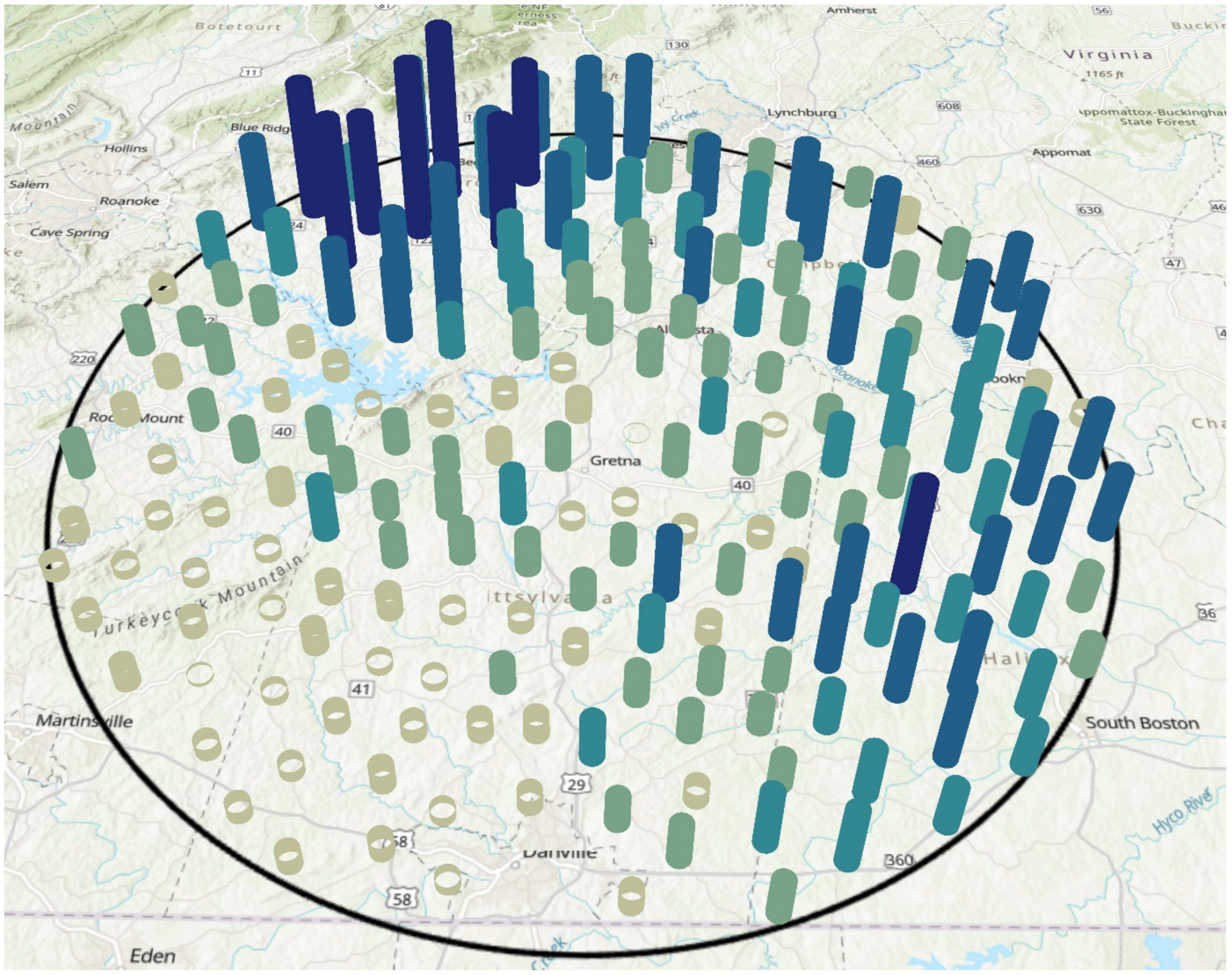
A 6-month (24-week) harvest schedule (September to February) at the start of the 48-week load-out operation was selected to emulate the schedule studied by Cundiff et al. [19]. This study used a database of potential production fields within a 50 km radius of Gretna, VA (the “Gretna database”) [18]. The locations of 199 SSLs for this distribution of production fields were sited heuristically [18]. The relative amount of assumed feedstock placed in each SSL is shown in Figure 1. Based on the distribution of production fields found in the aerial photographs used to develop the database, the production of feedstock across the region was not uniform [18]. This is expected for any area like the Virginia Piedmont with diverse land use.
The production database assumed that 40% of the potential production fields in the Gretna database could be attracted into feedstock production [18]. The total feedstock stored in all SSLs was 152,526 Mg (Figure 1). A biorefinery processing this material over 48 weeks of annual operation must average 3178 Mg/wk (454 Mg/d or 386 dry Mg/d at 15% moisture content [20]). For 24/7 operation, this equates to 18.9 Mg/h or, for bales averaging 0.4 Mg, about 47 bales/h.
A biorefinery processing 386 dry Mg/d is about 20% of the DOE’s optimum biorefinery capacity [10]. A biorefinery of this size would require five, or more, preprocessing depots to supply feedstock pellets to operate an optimum biorefinery. Whether the truck delivery of baled feedstock is direct to a biorefinery or to a preprocessing depot, the same principles and operating parameters apply; thus, this study is applicable.
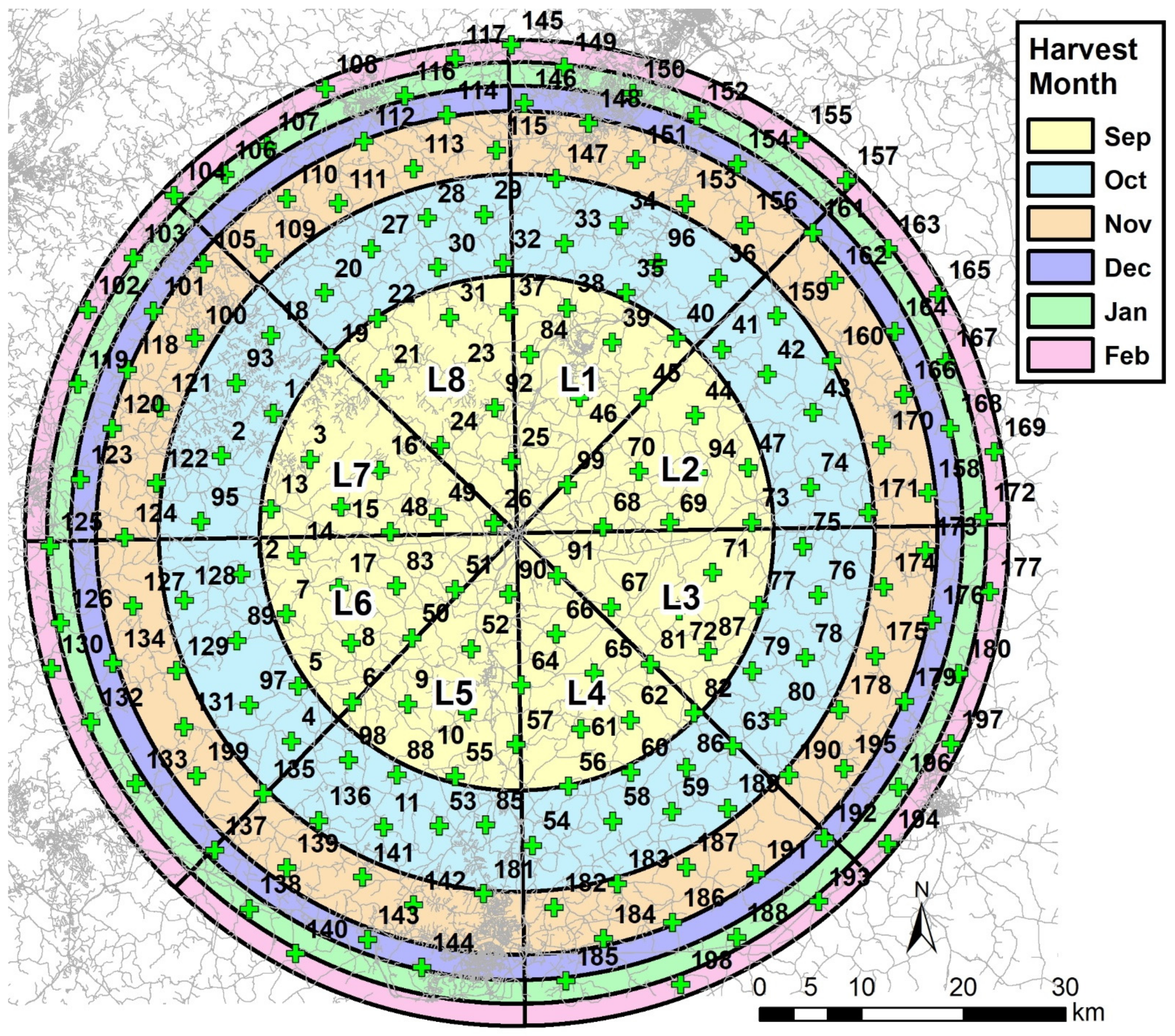
In a real-life operation, the harvest month for any SSL could be random depending on the feedstock contract agreed to by the biorefinery and contract holder. This agreement would be put in place before the start of annual operations on 1 September. For this study, an initial assignment of harvest months was predefined (Figure 2). This harvest plan was selected to provide a starting point, not to recommend a plan for a commercial operation. Approximately 27% of the area in the 50 km radius is in the September circle. The annular ring for the October harvest is about 26%, about 20% for the November harvest, and about 9% each for the December, January, and February harvests.
2.2. Description of Harvest Operations
In practice, farmgate contractors will harvest during the month called for in their contract. For example, if they have a September contract, their goal is to complete harvest by the end of September. When complete, they inform the feedstock manager of the estimated number of bales in storage at their SSL. The filling schedule for an individual SSL in this study was assumed. For the September harvest, the smaller SSLs were assumed to be filled on either week 1, 2, 3, or 4. Midsize SSLs were filled over a 2-week period, and the larger SSLs were filled over a 4-week period. This same procedure was followed for the other harvest months.
The maximum harvest rate used for the fill schedule at a single SSL was 400 Mg/wk. For round bales averaging 0.4 Mg, this equates to 1000 bales/wk. If the yield is 6.7 Mg/ha [21], the total production area harvested is about 60 ha/wk, which is more than what can be harvested with a single baler; thus, the fill schedule used for the larger SSLs will require more than one harvesting operation operating simultaneously.
The result of the assumed fill schedule was a matrix (199 SSLs × 24 weeks) defined as SSLin jk, where j is the jth SSL and k is the kth week in a 24-week harvest season within the 48-week load-out operation. The positions in this matrix for weeks 25 to 48 (i.e., after harvest is complete for the year) were set to zero.
2.3. Description of Load-Out Operations
Simulations were performed for 8, 9, and 10 load-out operations operating simultaneously. A load-out operation was defined as the 48-week period when feedstock from the SSLs is shipped to the biorefinery [12]. A truckload was defined as 40 round bales, two 20-bale racks on tandem trailers [15]. Assuming 0.4 Mg/bale, the average truckload would be 16 Mg. A truck arrives at the SSL, unhooks the tandem trailers with two empty racks, and hooks the loaded trailers, an operation that emulates the logging industry [22,23].
An ideal load-out productivity was defined as six loads/d for a 6-day workweek. On certain days, an operation might do six loads, but on other days, it might be more or less. For example, on a day when an operation finishes unloading one SSL, then moves to the next SSL in the schedule, the total loads will be fewer. This study assumed that operations, excepting winter days when roads are impassible due to ice or snow, and days when an equipment breakdown stops operation, can average 70% of the ideal productivity. This percentage is often used by custom operators to estimate their achieved productivity with a unit of agricultural equipment in a production setting.
2.4. Description of Load-Out Simulations
2.4.1. Eight-Load-Out Simulation
The eight-load-out simulation was defined by equal-size subareas (Figure 2). This method was chosen as one way a load-out might be assigned; it was not an optimized selection. The load-out sequence in each subarea starts with the September harvest SSLs and proceeds to the October SSLs and so forth to complete the hauling for all SSLs. The procedure follows the general delivery rule, “first in, first out”, and ensures that an SSL is full when load-out is scheduled.
Ideal productivity was defined as (16 Mg/load) (6 loads/d) (6 d/wk) = 576 Mg/wk. Preliminary analysis determined that eight load-outs would need an average productivity equal to 72.2% of the ideal setting, (576 Mg/wk) (0.722) = 415.8 Mg/wk, to complete shipment of all feedstock in 49 weeks. If a move between SSLs occurs, then the estimated time required would be 0.5 day [13]. The achieved average productivity for that week, compared with a normal week, would be (415.8 Mg/d) (5.5/6) = 381.2 Mg/wk.
Explanation of the load-out schedule for the individual load-out operations is best performed with an example. This example uses SSLs 46, 45, and 84 from the load-out 1 schedule and begins with operations in week 3. At the beginning of this week, there is 269.1 Mg remaining of the total feedstock stored in SSL 46. The operation loads out this feedstock and moves to SSL 45, which has 740.5 Mg stored. The amount shipped from SSL 45 to complete week 3 operations (i.e., a week when a move between SSLs occurs) is:
381.2 − 269.1 = 112 Mg
The amount shipped in week 4 from SSL 45 is the average productivity of 415.8 Mg. The amount shipped in week 5 is the total stored at SSL 45 minus previous shipments.
740.5 − 112 (Week 3) − 415.8 (Week 4) = 212.7 Mg
The operation loads out this feedstock and moves to SSL 84, which has 578.3 Mg stored. The amount shipped from SSL 84 to complete week 5 operations is:
381.2 − 212.7 = 168.4 Mg
The calculations proceed in this manner until all 20 SSLs in the load-out 1 schedule are shipped. With this procedure, the load-out operations achieve about the same average productivity across the entire 49 weeks of operation. An estimated productivity factor of 72.2% is optimistic, particularly for the start-up period when the industry is being established. It is also optimistic to expect a load-out operation to achieve the same productivity across 49 weeks of operation. The eight-load-out simulation was used as a baseline estimate of load-out productivity.
The result of the load-out assignment was a matrix (199 SSLs × nwk weeks) defined as SSLout jk, where j is the jth SSL and k is the kth week in an nwk-week load-out season. For the eight-load-out simulation, nwk = 49. Feedstock in storage in the jth SSL at the end of the kth week was calculated as:
This calculation was repeated for each SSL to obtain the feedstock stored at the end of the kth week. The 9- and 10-load-out simulations did not consider the fill schedule (i.e., an SSL was assumed to be full when it appeared on the load-out schedule); thus, the amount in storage was not calculated for these two simulations.
2.4.2. Nine-Load-Out Simulation
The eight-load-out simulation had a major flaw. All load-outs started at the closest SSL to the biorefinery and proceeded to the outermost SSL. This means that the truck fleet to service all load-outs was smallest at the beginning of the season (when each SSL has a small truck cycle time) and greatest at the end (when each truck has a large cycle time). The most efficient use of the truck fleet is achieved when a given number of trucks can be operated with each truck achieving approximately the same average operating time each week over the season.
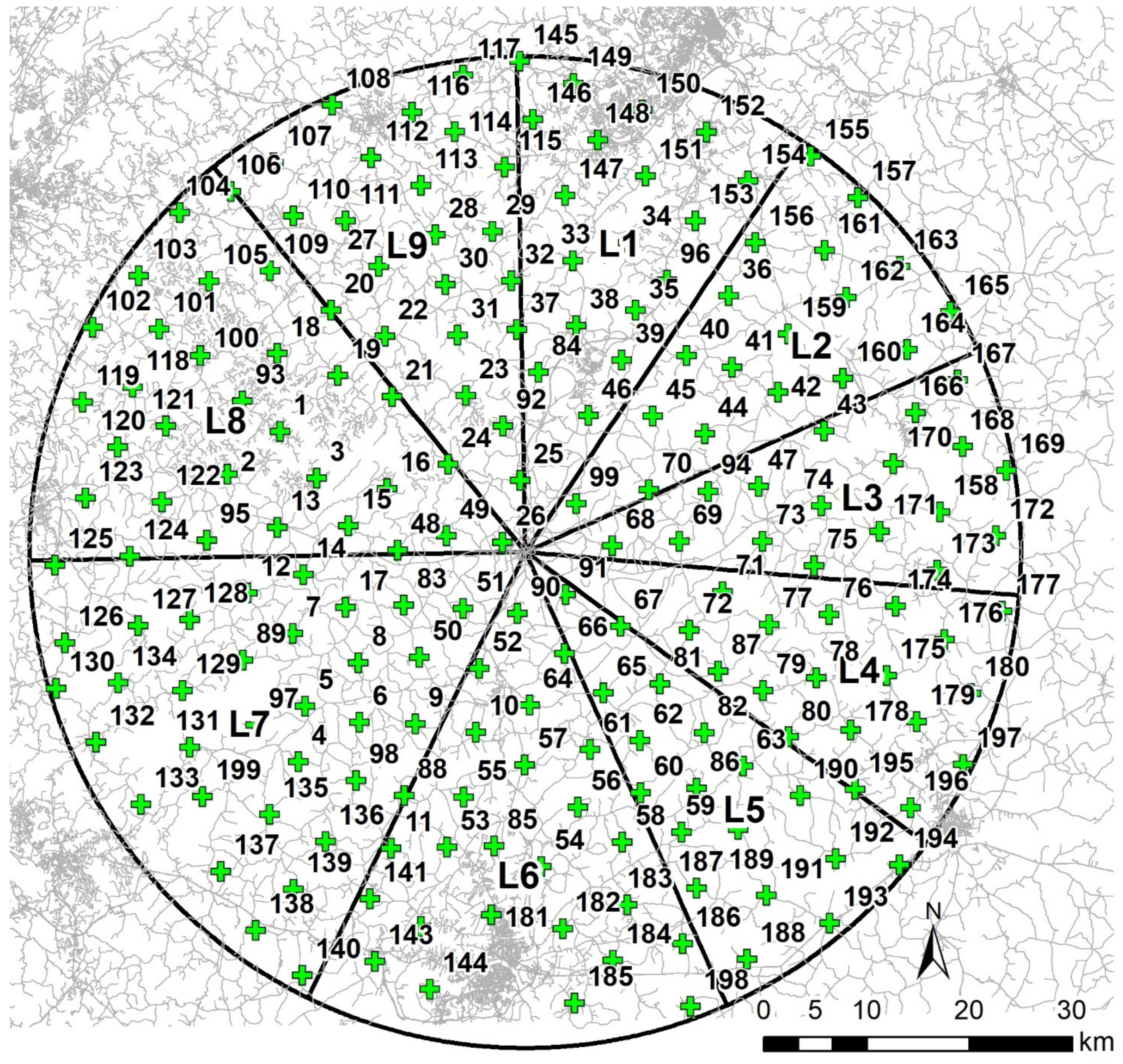
The nine-load-out simulation used the subareas defined in Figure 3. The subareas were optimized using a simple “greedy” algorithm. The subareas started as equal size, like before, but then the subarea with the most feedstock was reduced in size, and the subarea with the least feedstock was grown. After multiple iterations, each subarea had approximately the same amount of stored feedstock. The locations of the SSLs, total area of production fields, and amount of feedstock in each SSL were the same as for the eight-load-out simulation.
The load-out sequences were also modified to achieve approximately equal truck operating hours each week. The following schedule was assigned, where “in-to-out” means that the load-out sequence starts near the biorefinery and proceeds outward, while “out-to-in” means that the sequence starts at the outer boundary and proceeds toward the biorefinery. Subareas L1, L3, L5, and L7 were “in-to-out”, and L2, L4, L6, L8, and L9 were “out-to-in” (Figure 3).
In actual practice, the “harvest date” for SSLs will most likely be randomly distributed and an important parameter for the feedstock manager. The sequence chosen here simply directs the various load-outs to move to the next nearest SSL in their subarea. A productivity factor of 70% was used for this simulation. The achieved average productivity was 403.2 Mg/wk for a 6-day week and 369.6 Mg/wk for a 5.5-day week (i.e., when a move between SSLs occurs).
2.4.3. Ten-Load-Out Simulation
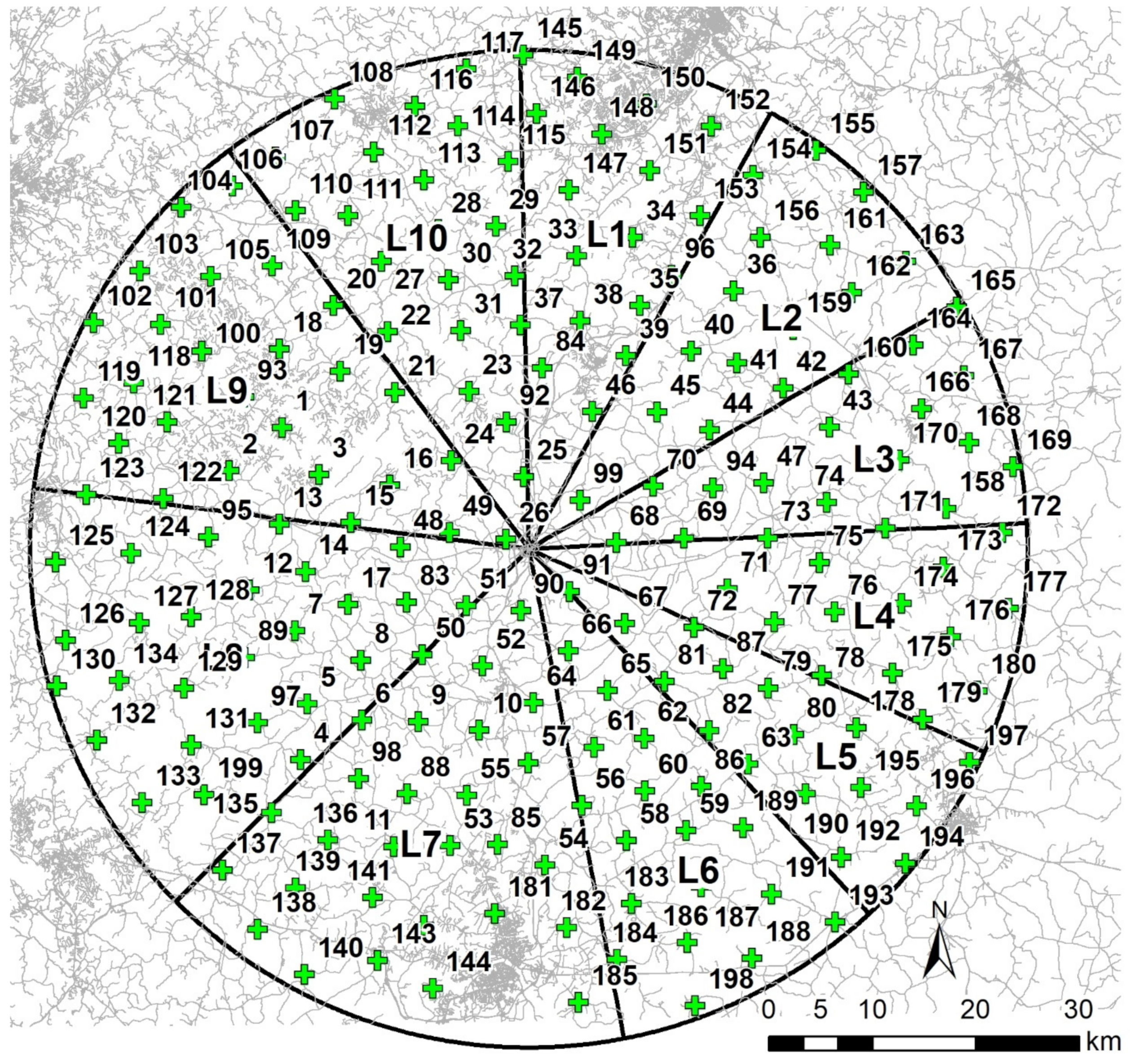
The 10-load-out simulation was performed using the subareas defined in Figure 4. As with the 9-load-out simulation, the subareas were optimized to have about the same total feedstock storage. The productivity factor used for this simulation was 60%, as this was judged to be more realistic for a start-up industry. The achieved average productivity was 345.6 Mg/wk for a 6-day week and 316.8 Mg/wk for a 5.5-day week (i.e., when a move between SSLs occurs). The same load-out sequencing procedure used for the 9-load-out simulation was used for the 10-load-out simulation. Subareas L1, L3, L5, L7, and L9 were “in-to-out”, and L2, L4, L6, L8, and L10 were “out-to-in” (Figure 4).
2.4.4. Summary of Load-Out Simulation Parameters
Based on the above descriptions of the three load-out simulations (8, 9, and 10), the parameters for each are summarized in Table 1. Despite the best efforts of the feedstock manager, there will always be viability in the daily delivery rate. The number of weeks (nwk) was allowed to vary as required for each simulation (Table 1). The simulations did not provide for a stored supply of feedstock to fill in weeks less than 48. No penalty was assigned if the biorefinery ran out of feedstock before 48 weeks or had to extend operations beyond 48 weeks.
In a production setting, the amount of harvested feedstock from the total production area will be different each year. A good growing season will produce higher yields, and the farmgate contractors will want to sell all the feedstock they produce. Conversely, a dry year will produce lower yields, and the farmgate contractors will not want to be penalized for not meeting their contract. This issue was not addressed here, but would need to be addressed by future studies before a commercial industry is built.
2.5. Description of Truck Hauling
For the biorefinery to process all harvested feedstock, the processing rate must average 3178 Mg/wk. An average truckload is 16 Mg; thus, the biorefinery must receive, on average, 199 truckloads/wk, or 33 truckloads/d for a 6-day workweek. For a 12 h workday, the receiving rate must be about 3 loads/h, which is a truckload every 20 min. A truck crosses the scale, the load is sampled for quality, it is unloaded, and then it crosses the scale to exit.
The total truckloads stored at each SSL were determined by dividing the stored feedstock by 16 Mg to obtain nlj, the number of loads stored at the jth SSL. This number was rounded down to the next lowest integer to eliminate the possibility of a partial load.
An estimate of the total haul distance by the truck fleet was computed as:
where:
hdtot = total distance (round trip) traveled by truck fleet (km);
hdj = road distance from the jth SSL to biorefinery (km);
nlj = number of loads at the jth SSL.
The total haul distance traveled by the truck fleet for the kth week was calculated as:
where:
hdk = total distance (round trip) traveled by truck fleet during the kth week (km);
SSLout jk = feedstock shipped from the jth SSL in the kth week (Mg).
The number of loads ( was rounded down to eliminate partial loads. The SSLout jk value was defined as zero for all weeks except the weeks when shipments were made.
A mass–distance parameter for feedstock delivered to the biorefinery was defined as:
where:
paramd = mass–distance parameter (km);
mj = mass of feedstock stored in the jth SSL (Mg);
The truck cycle time was calculated for each SSL using three assumptions:
- The truck average velocity over rural roads (delivery and return) is 70 km/h;
- The truck load time (Lt) averages 15 min. This is the time to unhook the two empty rack trailers and hook the two loaded rack trailers at the SSL;
- The truck unload time (Ut) averages 20 min. This is the time to weigh in a load, sample for quality, unload the racks, load two empty racks, and weigh out.
The ideal truck cycle time (i.e., assuming no delays) was computed as:
where:
Tcyc j = ideal cycle time to haul from the jth SSL (h);
Lt = load time (min);
Ut = unload time (min);
hdj = haul distance over existing roads from the jth SSL to the biorefinery (km).
A well-run logistics system was estimated to average 1.4 times the ideal cycle time in a real-life operation. Thus, the total truck operating hours to haul all loads from the 199 SSLs was calculated as:
where:
nlj = number of loads at the jth SSL.
A single truck operating 12 h/d, 6 d/wk for 48 weeks will operate 3456 h in a season. A crude method to estimate the number of trucks is to sum the required operating hours for each week of the nwk season and divide by the total hours operated by a single truck:
The assignment of a given truck to a given load-out is not a viable option. For example, the haul distance for SSL 26 is 3.1 km; thus, in a 12 h haul day based on an ideal cycle time, a single truck could haul 12.8 loads. SSL 198 has a haul distance of 69.8 km; thus, a single truck could haul 3.3 loads. A load-out operation, in an ideal setting, might be able to achieve 10 loads in a 10 h workday, but 12.8 loads is not practical. A load-out with ideal operations would be expected to average 6 loads/d. This means that the truck serving SSL 26 would spend part of the day waiting for loading to be completed. Conversely, the load-out operation at SSL 198 would spend much of the day waiting for a truck to arrive.
2.6. Description of Central Control Plan
The required truck operating hours each week of the nwk operating season is given by:
As explained in Equation (3), ( is the number of loads hauled from SSL j during week k. Equation (8) gives the total truck operating hours to haul all feedstock being loaded out during the kth week. This was identified as a key operating parameter. If central control can implement a plan to achieve approximately the same truck operating hours each week, this will provide the minimum truck fleet size needed to haul all feedstock that week, assuming that all load-out operations are operating at the expected productivity.
It is likely that a “clean-up” operation will visit each SSL after it is unloaded to haul the remaining material. The number of bales hauled by the clean-up will range from 1 to 40 and will include damaged bales. The need for a clean-up operation is obvious because a feedstock contract holder will expect to be paid for the total feedstock he or she produces.
Suppose that the minimum farmgate contract is 25 ha and the average yield is 6.7 Mg/ha. The total stored in the SSL is 25 × 6.7 = 167.5 Mg. For bales averaging 0.4 Mg/bale, this storage is 167.5/0.4 = 419 bales. At 40 bales/load, this equals 10 loads plus 19 bales left for the clean-up crew. For each simulation, the total amount (in all SSLs) left for the clean-up crew was calculated and reported as a percentage of the total stored feedstock.
2.7. Description of Cost Analysis
2.7.1. Load-Out Operation Cost
Grisso et al. [12] estimated the cost to operate a telehandler as 41.55 USD/h and the cost to operate a bale loader, used to load bales into the 20-bale rack, as 10.32 USD/h. These costs assumed that one operator operates both the telehandler and the bale loader (by remote control). Labor cost was based on 10 h/d, 6 d/wk, 48 wk/y, or 2880 h/y. Labor cost for the load-out operator was 25 (base) [1 + 0.25 (benefits)] = 31.25 USD/h.
For this analysis, the labor hours are continuous, but the equipment operating hours are reduced to account for the time the equipment is actually operating. Annual equipment operating hours are calculated as follows, and equipment cost is based on this annual use:
where:
Loh = load-out equipment operation (annual operating h);
Lh = load-out labor (annual operating h);
prodf = achieved load-out productivity factor for each simulation.
2.7.2. Service Truck Cost
Two service trucks are specified to support the load-out operations. The technicians in these trucks will provide fuel, maintenance, and support to the load-outs. The ownership and operating cost (labor not included) for a service truck is 1.85 USD/km [13]. The annual travel was estimated by assuming that a service truck will visit each SSL being unloaded each workday (e.g., eight SSLs for eight load-outs). The distance between SSLs was drawn from a database. This calculation is made for the SSLs being loaded out on the Monday of each workweek. For example, during week 10 of the eight-load-out simulation, eight SSLs are unloaded, and each is visited six times.
The scheduling of service calls at each active SSL is a classic “traveling salesman problem” [24]. In commercial practice, the feedstock manager will optimize the travel of the service trucks. Here, the simulation took the load-out SSLs in sequence, for example, load-out 1 to load-out 8. The labor cost for two service technicians is calculated as follows for the eight-load-out simulation:
2.7.3. Equipment Hauler Cost
The simulations assume that one equipment hauler will move all the load-out operations between SSLs. The equipment hauler is based at the biorefinery and is dispatched when needed [25]. Equipment is hauled to the first SSL to begin the season and hauled from the last SSL back to the biorefinery at the end of the season. The eight-load-out simulation is used as an example. The load-out number is followed by the number of moves between SSLs in parenthesis: L1 (19), L2 (18), L3 (18), L4 (22), L5 (29), L6 (30), L7 (31), and L8 (25) for a total of 192 moves over the 49-week season. On average, the equipment hauler must complete 3.9 moves per week. For the 9-load-out simulation, the equipment hauler must complete 190 moves in 46 weeks, an average of 4.1 moves per week. The 10-load-out simulation requires 189 moves in 47 weeks, an average of 4.0 moves per week.
The scheduling of the equipment hauler will be the responsibility of the feedstock manager [25]. A load-out operation should not lose time while waiting to be moved to the next SSL. Scheduling has a significant influence on the achieved average load-out productivity, particularly for smaller SSLs. Planning by central control at the biorefinery can ensure that the equipment hauler arrives when needed.
Cundiff and Grisso [13] estimated a cost factor of 3.10 USD/km (labor included) for the equipment hauler. The annual travel for the total moves was calculated by adding (distance to current SSL) + (distance to the next SSL) + (return distance to the biorefinery). This procedure may overestimate the total travel because the equipment hauler may, on certain days, complete two load-out moves before returning to the biorefinery.
2.7.4. Truck Cost
Truck cost was calculated using the procedures given in Cundiff and Grisso [13]. The plan specifies that the biorefinery leases truck tractors and owns the trailers. Drivers are hired by the biorefinery, and the trucks are fueled at the biorefinery. All other operating costs are included in the lease. Repeating the central control constraint, the feedstock manager at the biorefinery will dispatch any truck to any SSL where a load will be ready when the truck arrives.
The truck cost includes the truck tractor rental, driver, and fuel. No cost is included here for the trailers and racks or for receiving facility operations. The rental cost for a single-axle, pintle-hitch truck tractor is 845 USD/wk. For example, the annual truck cost required for the eight-load-out simulation (i.e., a 49-week season) is:
The labor cost for an operator is 31.25 USD/h. A shift-work plan must be used to operate a 12 h haul day, 6 d/wk. The annual labor cost (49 wk/y) is 110,250 USD per truck per year.
3. Results and Discussion
3.1. Load-Out Simulation Results
3.1.1. Eight-Load-Out Simulation
For the eight-load-out simulation, the number of SSLs ranged from 19 (load-outs 2 and 3) to 32 (load-out 7). Contingency days, defined as the days remaining in a 49-week season after all SSLs are unloaded, ranged from 0 (load-out 6) to 10 (load-outs 3 and 5). The total number of contingency days was 30, or an average of about 4 days per load-out. The average productivity used for the simulation was 69.3 Mg/d (Table 1). The achieved average productivity, considering the 0.5 day to move between SSLs, ranged from 64.5 Mg/d for load-out 7 to 68.5 Mg/d for load-out 3 (Table 2). The low productivity for load-out 7 is partly explained by the 32 moves between SSLs (i.e., 16 days of lost productivity). The high productivity for load-out 3 is due to the higher mass moved over the 49-week season (19,370 Mg) as compared with an average of 19,066 Mg across all eight load-outs.
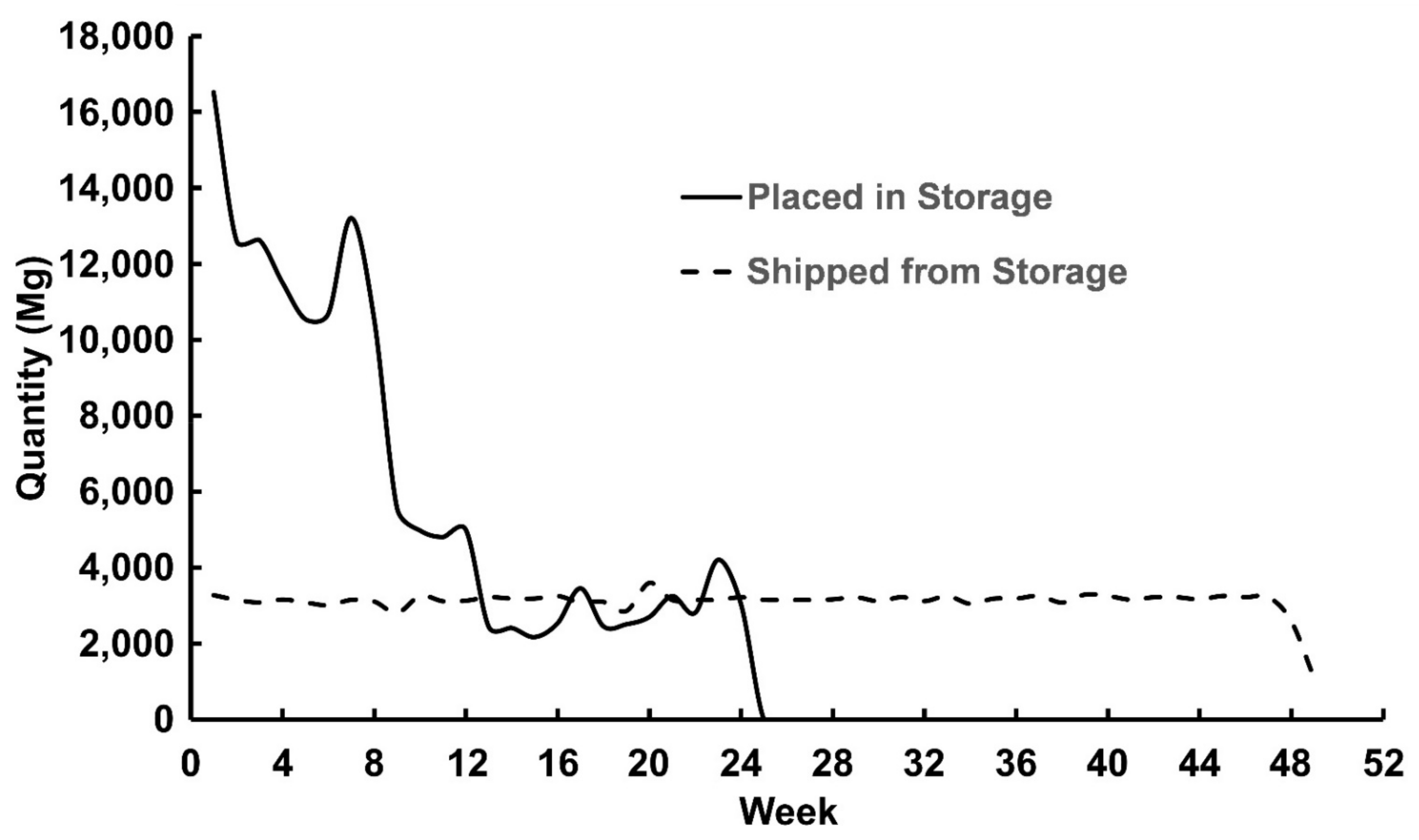
The total feedstock placed in storage each week of the 24-week harvest season, and loaded out each week over the 49-week season, is given in Figure 5. The total delivered by the eight load-outs was 9174 loads × 16 Mg/load = 146,764 Mg, leaving 3.8% of the 152,526 Mg placed in storage to be hauled by the clean-up crew. In a real-life harvest season, the peaks and valleys in the quantity placed in storage will track the weather patterns. A week with good harvest weather will have large quantities harvested and placed in storage; a rainy week may have no harvest. A modest attempt was made to emulate this variability when the SSLin matrix was created.
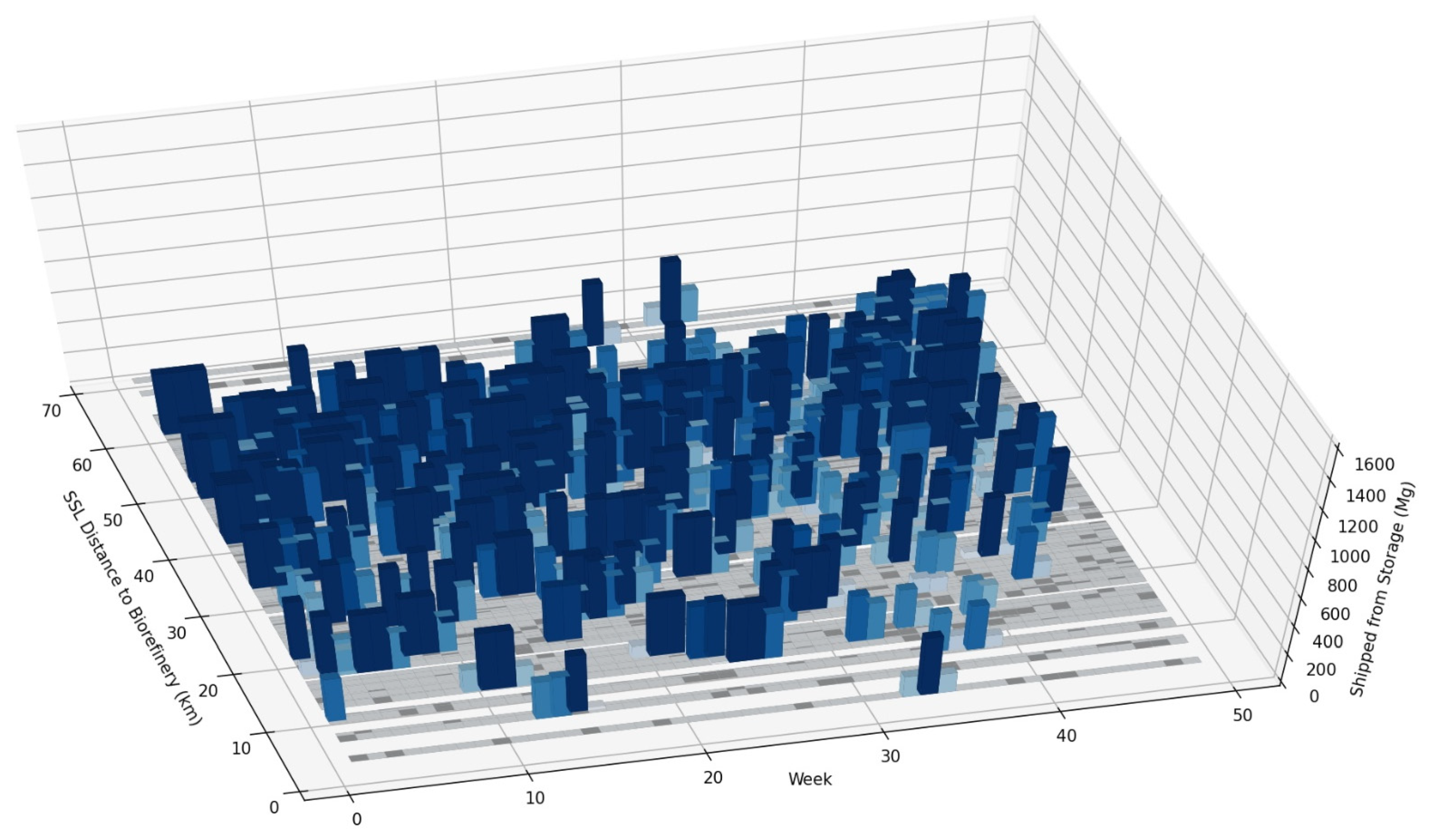
The SSLout matrix was created so each load-out operation would deliver approximately the same feedstock each week, producing an approximately uniform delivery for each week in the 49-week season (Figure 5). A commercial system with eight load-out operations would be expected to have more variability in the weekly delivery curve. To visualize the simulation output, the amount of feedstock shipped from each SSL for each week in the 49-week season is shown in Figure 6. The height of the bar graph is the amount of feedstock shipped to the biorefinery from that SSL for a given week, with the maximum height representing an average productivity of 415.8 Mg. This figure is included to attempt to show some of the spatial complexities of distributed feedstock storage and the need for central control to organize the delivery of feedstock evenly throughout the production zone.
3.1.2. Nine-Load-Out Simulation
For the nine-load-out simulation, the number of SSLs ranged from 16 (load-out 3) to 28 (load-outs 6 and 7), and contingency days ranged from 12 (load-out 2) to 35 (load-out 9). The total number of contingency days was 218, or an average of about 24 days per load-out. The average productivity used for the simulation was 67.2 Mg/d (Table 1). The achieved average productivity, including moves between SSLs, ranged from 62.8 Mg/d (load-out 7) to 67.3 Mg/d (load-out 1) (Table 3). The low productivity for load-out 7 is explained by the 28 moves between SSLs (i.e., a loss of 14 days). The high productivity of load-out 1 is due to the higher mass moved over the 46-week season (17,829 Mg) as compared with an average of 16,947 Mg across all nine load-outs.
The total loads delivered with the nine-load-out simulation was 9321 as compared with 9174 with the eight-load-out simulation. The number of moves between SSLs for the eight load-outs averaged 23.9 moves/load-out as compared with 21.1 for the nine load-outs. This led to fewer partial loads over the season. The total feedstock hauled by the nine-load-out simulation was 149,136 Mg, leaving 2.2% for clean-up.
3.1.3. Ten-Load-Out Simulation
A summary of the results for the 10-load-out simulation is given in Table 4. For the 10-load-out simulation, the number of SSLs ranged from 14 (load-out 4) to 28 (load-out 7), and the contingency days ranged from 7 (load-outs 7, 9, and 10) to 21 (load-out 6). The total number of contingency days was 128, or an average of about 13 days per load-out. The achieved average productivity, including moves between SSLs, ranged from 54.3 Mg/d (load-out 8) to 56.9 Mg/d (load-out 4) (Table 4). The low productivity for load-out 8 is partly explained by the 25 moves between SSLs (i.e., a loss of 12.5 days).
The total number of loads delivered with the 10-load-out simulation was 9197, approximately the same as the 9174 loads with the 8-load-out simulation. The number of moves between SSLs for the 10 load-outs averaged 18.9 moves/load-out as compared with 21.1 for the 9 load-outs and 23.9 for the 8 load-outs. The total feedstock hauled by the 10-load-out simulation was 147,152 Mg, leaving 3.5% for clean-up.
3.2. Required Truck Operating Hours
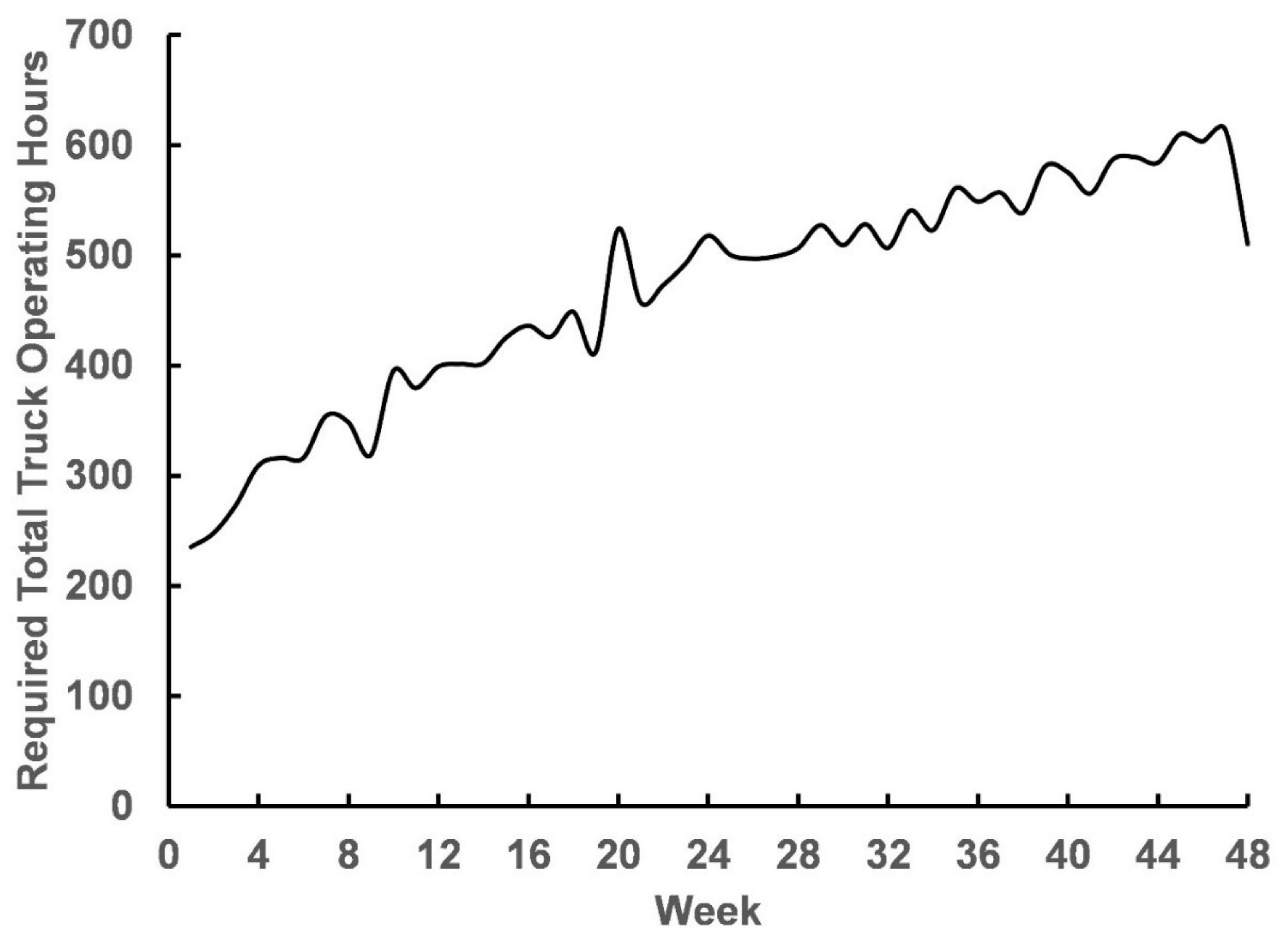
The weekly truck operating hours for the eight-load-out simulation is given in Figure 7. The minimum was 235.1 h (week 1), and the maximum was 614.2 h (week 47). Each truck is available for (6 d) (12 h/d) = 72 h/wk; thus, the minimum number of trucks was 3.3, and the maximum was 8.5. This management plan would require nine trucks to ensure that the total hauling requirement can be met each week; this is not an optimum plan. Ideally, operations would be managed, and an SSL unload sequence chosen, such that approximately the same number of trucks is required for each week of operation.
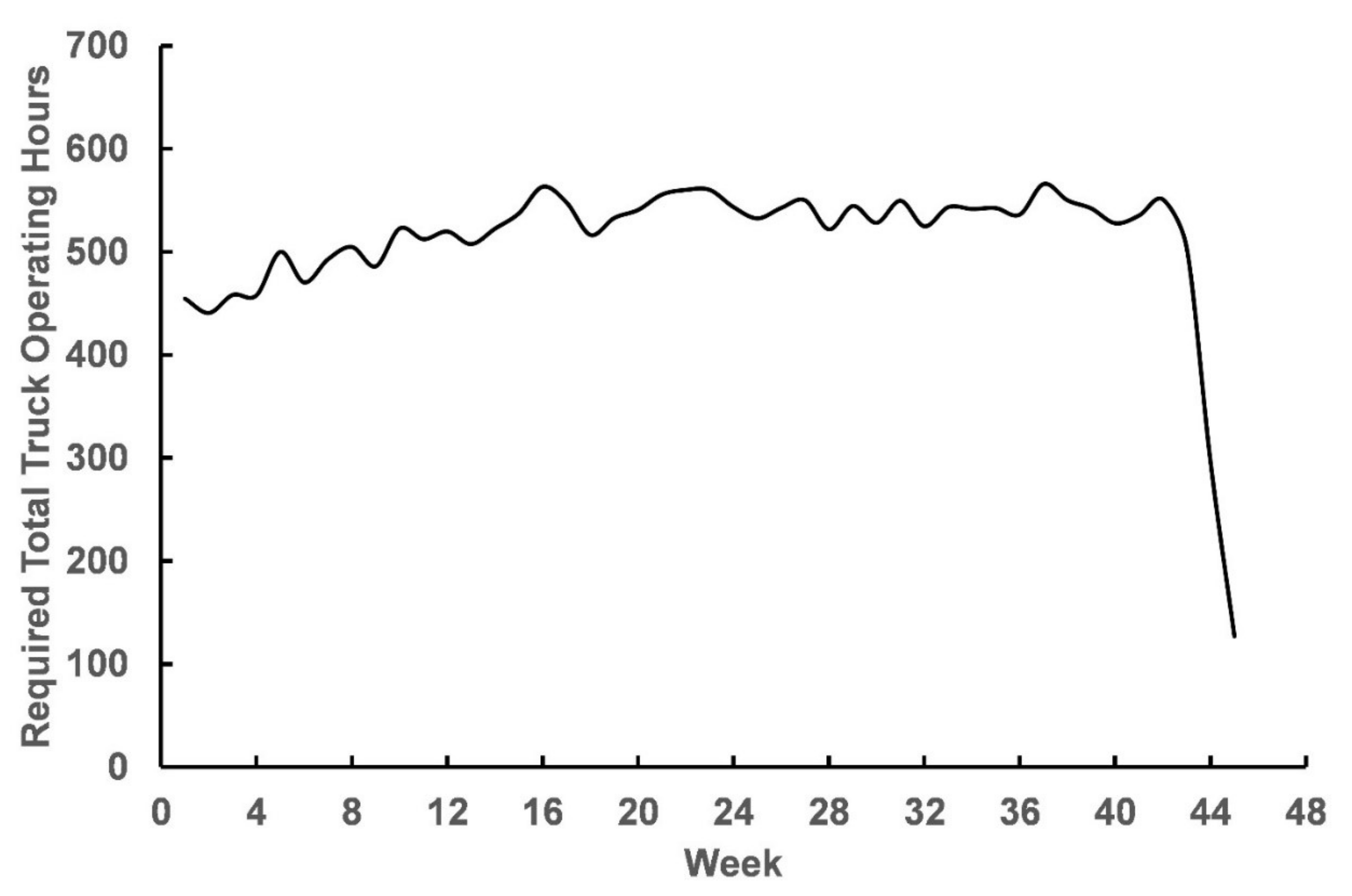
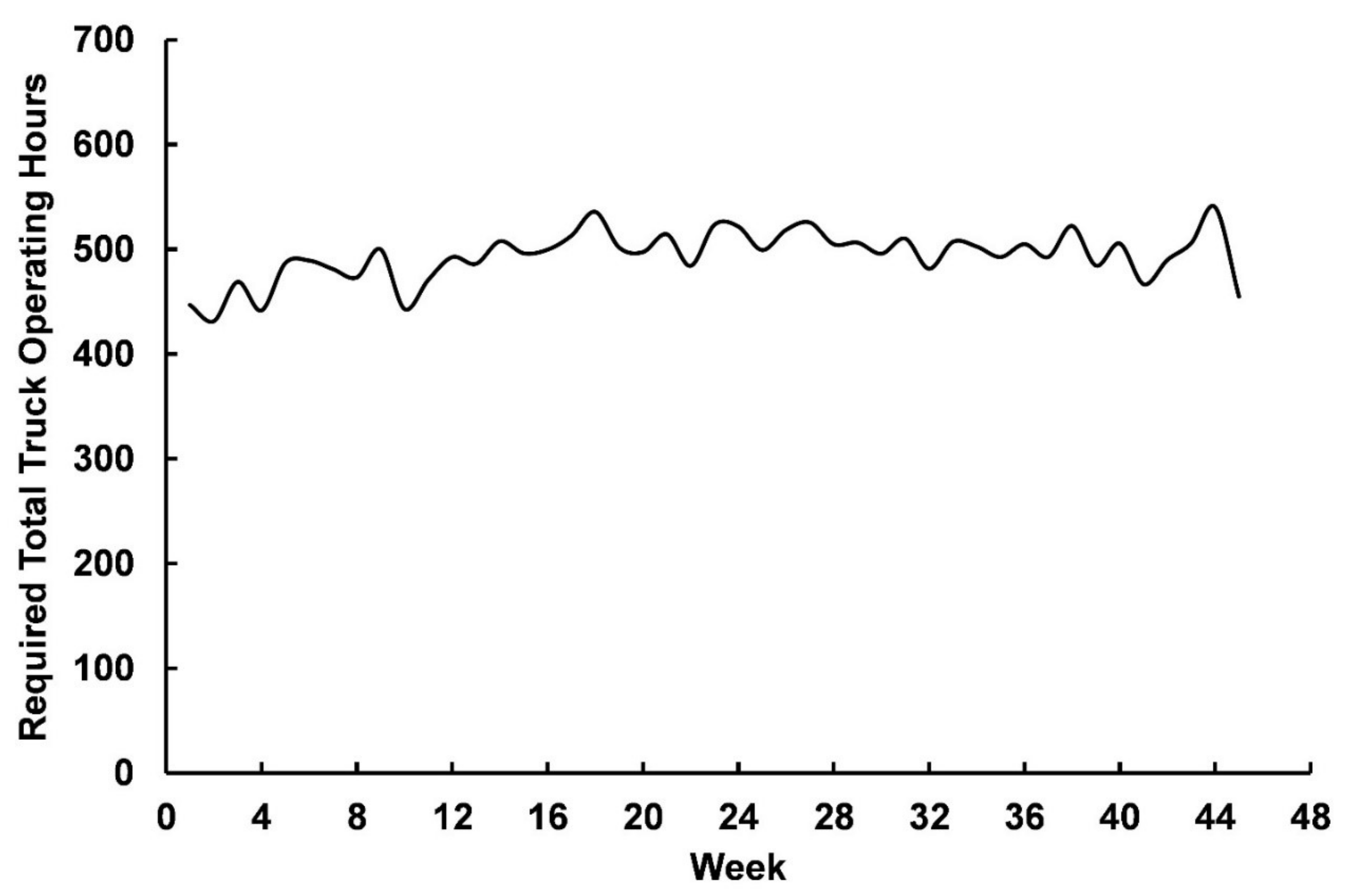
The weekly truck operating hours for the nine-load-out simulation is given in Figure 8. The minimum was 440.7 h (week 2), and the maximum was 565.8 h (week 37); thus, the minimum number of trucks was 6.1, and the maximum was 7.9. This management plan increases the average productivity of each truck and reduces the maximum number of trucks required from nine (for the eight-load-out simulation) to eight.
The weekly truck operating hours for the 10-load-out simulation is given in Figure 9. The minimum was 431.4 h (week 2), and the maximum was 535.7 h (week 18); thus, the minimum number of trucks was 6.0, and the maximum was 7.4. This management plan does not reduce the maximum number of trucks required below that calculated for the nine-load-out simulation (i.e., eight).
3.3. Cost Analysis Results
3.3.1. Cost to Load Trailers at an SSL
The eight load-outs hauled 146,784 Mg over a 49-week season, and the nine load-outs hauled 149,136 Mg over a 46-week season. The difference in total feedstock is due to the number of loads, 9174 as compared with 9321, and the difference in loads is due to the round-down procedure. The 10 load-outs shipped 147,152 Mg (9197 loads) over a 47-week season. The computation of cost per Mg was based on the total feedstock hauled. The feedstock left for clean-up operations was 3.8%, 2.2%, and 3.5%, for the 8-, 9-, and 10-load-out simulations, respectively.
The total service truck and equipment hauler travels for each simulation (Table 5) were used to calculate service truck and equipment hauler costs (Table 6). For example, the total service truck travel for the eight-load-out simulation was 94,245 km; thus, the total truck cost was 94,245 km × 1.85 USD/km = 174,354 USD (for 2 trucks) + 183,750 labor (for 2 technicians) = 358,104 USD, or 2.37 USD/Mg. The total travel for the equipment hauler was 19,715 km; thus, the cost was 61,120 USD or 0.41 USD/Mg.
3.3.2. Cost of Truck Operations
Haul distance ranged from 3.1 km (SSL 26) to 62.6 km (SSL 117) with a mean of 40.7 km across all 199 SSLs. The mass–distance parameter was found to be 41.4 km, meaning that each delivered Mg was hauled at an average of 41.4 km.
The total haul distance for each simulation based on the number of loads hauled from each SSL, rounded down as described in Equation (2), is given in Table 7. The fuel cost (based on 1.7 km/L at 1.31 USD/L) was given as USD/Mg annual delivery. The calculated fuel cost (on a USD/Mg basis) was about the same for all the three simulations.
The total number of loads hauled was different for each simulation because of load rounding. The number of loads shipped from a given SSL was rounded down for each week the SSL was unloaded; thus, the total remaining material was greater than what would be left by a real-life operation. For example, if the unloading is done over a 3-week period, a residue (i.e., partial load) is calculated for each week. In actual operations, the only partial load will be left at the end of the third week when operations at that SSL are concluded. The amount left at each SSL will always be less than 16 Mg. For the eight-load-out simulation, the total left was 5742 Mg, and the total number moves was 191; thus, the average left material was 30.0 Mg/move. The results for the 9- and 10-load-out simulations were 17.8 and 28.4 Mg/move, respectively.
The truck cost was lowest for the 9-load-out simulation because the truck productivity was highest (Table 8). For the 8-load-out simulation, nine trucks hauled 146,784 Mg over 49 weeks (294 operating days), giving an average productivity of 57.4 Mg/d/truck. In the 9-load-out simulation, eight trucks hauled 149,136 Mg over 46 weeks (276 operating days), giving an average productivity of 67.5 Mg/d/truck or 17.6% higher than the 8-load-out simulation. The result for the 10-load-out simulation was eight trucks hauling 147,152 Mg over 47 weeks (282 operational days), giving an average productivity of 65.2 Mg/d/truck or 3.4% lower than the 9-load-out simulation. These results compare with the load-out productivities given in Table 2, Table 3 and Table 4.
3.3.3. Cost for Load-Out and Hauling
The total average delivered cost for each simulation, load-out plus truck hauling, is given in Table 9. It is important to observe that the load-out cost was approximately equal to the truck cost (i.e., rental, labor, and fuel). This is an important point that is often not appreciated. Obviously, the two operations, truck loading and hauling, are directly connected; thus, one cannot be optimized without the other. This fact is our key argument for central control (i.e., direct integration) of the two operations.
Minimum cost was achieved with nine load-outs and eight trucks (22.86 USD/Mg). If the central management was revised so that the eight-load-out simulation would require only eight trucks, the truck cost would be reduced to 12.25 USD/Mg, and the total cost to 23.42 USD/Mg. The difference is explained by the 49-week season for the eight-load-out simulation as compared with the 46-week season for the nine-load-out simulation.
Certain interesting questions can be proposed. Can the nine trucks be operated such that the eight load-outs can be operated at a higher productivity, more loads per day, and finish in 46 weeks? Will the resulting average cost be less than nine load-outs and eight trucks operating over a 46-week season? Is it best to have an extra truck so that the load-out delay between loads is reduced, or an extra load-out so that the number of loads per day per truck is increased? The costs of the racks, personnel, depot sampling processes (e.g., biomass quality and weight), and centralized control systems need to assessed. These questions outline needed future research.
3.4. Proposed Business Plan
Central control of hauling, defined as a plan to dispatch any truck to any SSL where a load is ready, provides an opportunity for the biorefinery to simultaneously maximize the productivity (Mg/wk) of both the loading and hauling operations. The proposed business plan for this study, the central control of feedstock hauling performed by the biorefinery, is used by the cotton and sugar industries in the Southeast. It should be implemented for a biorefinery industry for the same reasons that it is successful for these other herbaceous biomass industries.
This study uses the distribution of potential feedstock production fields and road travel haul distances between SSLs to calculate truck loading and hauling costs for a theoretical biorefinery in Gretna, VA. These two costs (in USD/Mg of annual operation) were determined to be approximately equal over 48 weeks of annual operation to collect feedstock from a 50 km radius around the biorefinery location (Table 9).
The simulations performed here use a heuristic selection of the SSL load-out sequence. There is a need for an optimization software to be used by the biorefinery to select the SSL load-out sequence for several load-out operations. This hypothetical software would run every Friday of the nwk-week season to guide the next weeks’ operation. The analysis would select from available filled SSLs (harvested over a 24-week season) and would consider the cost to move load-out operations from the current SSL to the SSL selected for the next week. For example, if the next SSL is selected on the opposite side of the production area, then equipment must be hauled at a greater distance and the mobilization cost (i.e., equipment hauling plus lost load-out time) will be greater.
4. Conclusions
This study demonstrated the potential of a central control model to optimize the delivery of switchgrass feedstock stored in SSLs to a theoretical biorefinery centered in Gretna, VA. Load-out simulations were performed using a database of fields and SSLs representing the potential production of feedstock within a 50 km radius of the theoretical biorefinery. The minimum delivered cost, calculated as load-out cost plus truck cost, was achieved with nine load-outs operating simultaneously with a fleet of eight trucks. The estimated cost was 11.24 and 11.62 USD/Mg of annual biorefinery capacity (assuming 24/7 operation, 48 wk/y, and a total production of approximately 150,000 Mg/y) for the load-out cost and truck cost, respectively. Interestingly, the two costs were approximately equal, emphasizing the need for central control to maximize the productivity of these two key operations.
The results of this study are applicable to the truck delivery of baled feedstock from SSLs directly to a biorefinery (of various capacities) or to a preprocessing plant (of various capacities). The recommended constraint is a production area defined by a 50 km radius around the receiving facility, although future work should explore the relationship between the size of the production area and the average delivered cost.
The production zone defined for this study covered parts of seven counties in southern Virginia and had an estimated annual production of approximately 150,000 Mg. The methodology described here for the central control model could easily be applied to other herbaceous biomass production zones. Resop and Cundiff [4] identified 34 potential multicounty production zones in the Piedmont region (spanning Virginia to Alabama) with estimated production ranging from 50,000 to 360,000 Mg, similar in size to the area defined for this study. Future research should apply the central control model to these other potential production zones and determine whether the optimal number of load-out operations varies between zones.
Author Contributions
Conceptualization, J.S.C.; methodology, J.S.C. and J.P.R.; software, J.S.C. and J.P.R.; validation, J.S.C. and R.D.G.; formal analysis, J.S.C.; investigation, J.S.C.; resources, J.S.C. and J.P.R.; data curation, J.P.R.; writing—original draft preparation, J.S.C. and J.P.R.; writing—review and editing, J.S.C., J.P.R. and R.D.G.; visualization, J.P.R.; supervision, J.S.C.; project administration, J.S.C.; funding acquisition, J.S.C. All authors have read and agreed to the published version of the manuscript.
Funding
This research received no external funding.
Institutional Review Board Statement
Not applicable.
Informed Consent Statement
Not applicable.
Data Availability Statement
Not applicable.
Conflicts of Interest
The authors declare no conflict of interest.
References
- Downing, M.; Eaton, L.M.; Graham, R.L.; Langholtz, M.H.; Perlack, R.D.; Turhollow, J.; Stokes, B.; Brandt, C.C. U.S. Billion-Ton Update: Biomass Supply for a Bioenergy and Bioproducts Industry; Oak Ridge National Lab (ORNL): Oak Ridge, TN, USA, 2011. [Google Scholar]
- Gonzales, D.S.; Searcy, S.W. GIS-Based Allocation of Herbaceous Biomass in Biorefineries and Depots. Biomass Bioenergy 2017, 97, 1–10. [Google Scholar] [CrossRef] [Green Version]
- Sharma, B.; Brandt, C.; McCullough-Amal, D.; Langholtz, M.; Webb, E. Assessment of the Feedstock Supply for Siting Single- and Multiple-Feedstock Biorefineries in the USA and Identification of Prevalent Feedstocks. Biofuels Bioprod. Biorefining 2020, 14, 578–593. [Google Scholar] [CrossRef]
- Resop, J.P.; Cundiff, J.S. Assessment of Herbaceous Feedstock Supply for Locating Biorefineries in the Piedmont, USA. Biofuels Bioprod. Biorefining 2022, 16, 43–53. [Google Scholar] [CrossRef]
- Mays, D.A.; Buchanan, W.; Bradford, B.N.; Giordano, P.M. Fuel Production Potential of Several Agricultural Crops. In Advances in New Crops; Janick, J., Simon, J.E., Eds.; Timber Press: Portland, OR, USA, 1990; pp. 260–263. [Google Scholar]
- Speight, J.G. 10-Non–Fossil Fuel Feedstocks. In The Refinery of the Future, 2nd ed.; Speight, J.G., Ed.; Gulf Professional Publishing: Houston, TX, USA, 2020; pp. 343–389. ISBN 978-0-12-816994-0. [Google Scholar]
- Schmer, M.R.; Vogel, K.P.; Mitchell, R.B.; Perrin, R.K. Net Energy of Cellulosic Ethanol from Switchgrass. Proc. Natl. Acad. Sci. USA 2008, 105, 464–469. [Google Scholar] [CrossRef] [PubMed] [Green Version]
- Hess, J.R.; Wright, C.T.; Kenney, K.L.; Searcy, E.M. Uniform-Format Solid Feedstock Supply System: A Commodity-Scale Design to Produce an Infrastructure-Compatible Bulk Solid from Lignocellulosic Biomass—Executive Summary; Idaho National Lab (INL): Idaho Falls, ID, USA, 2009. [Google Scholar]
- Carolan, J.E.; Joshi, S.V.; Dale, B.E. Technical and Financial Feasibility Analysis of Distributed Bioprocessing Using Regional Biomass Pre-Processing Centers. J. Agric. Food Ind. Organ. 2007, 5, 1–27. [Google Scholar] [CrossRef]
- Aden, A.; Ruth, M.; Ibsen, K.; Jechura, J.; Neeves, K.; Sheehan, J.; Wallace, B.; Montague, L.; Slayton, A.; Lukas, J. Lignocellulosic Biomass to Ethanol Process Design and Economics Utilizing Co-Current Dilute Acid Prehydrolysis and Enzymatic Hydrolysis for Corn Stover; National Renewable Energy Lab.: Golden, CO, USA, 2002. [Google Scholar]
- Morey, R.V.; Kaliyan, N.; Tiffany, D.G.; Schmidt, D.R. A Corn Stover Supply Logistics System. Appl. Eng. Agric. 2010, 26, 455–461. [Google Scholar] [CrossRef]
- Grisso, R.D.; Cundiff, J.S.; Sarin, S.C. Rapid Truck Loading for Efficient Feedstock Logistics. AgriEngineering 2021, 3, 158–167. [Google Scholar] [CrossRef]
- Cundiff, J.S.; Grisso, R.D. Load and Unload Technology to Improve Round-Bale Hauling Efficiency. AgriEngineering 2021, 3, 584–604. [Google Scholar] [CrossRef]
- Ravula, P.P.; Grisso, R.D.; Cundiff, J.S. Cotton Logistics as a Model for a Biomass Transportation System. Biomass Bioenergy 2008, 32, 314–325. [Google Scholar] [CrossRef]
- Grisso, R.D.; Cundiff, J.S.; Comer, K. Multi-Bale Handling Unit for Efficient Logistics. AgriEngineering 2020, 2, 336–349. [Google Scholar] [CrossRef]
- Parrish, D.J.; Fike, J.H. The Biology and Agronomy of Switchgrass for Biofuels. Crit. Rev. Plant Sci. 2005, 24, 423–459. [Google Scholar] [CrossRef]
- Persson, T.; Ortiz, B.V.; Bransby, D.I.; Wu, W.; Hoogenboom, G. Determining the Impact of Climate and Soil Variability on Switchgrass (Panicum virgatum L.) Production in the South-Eastern USA; a Simulation Study. Biofuels Bioprod. Biorefining 2011, 5, 505–518. [Google Scholar] [CrossRef]
- Resop, J.P.; Cundiff, J.S.; Heatwole, C.D. Spatial Analysis to Site Satellite Storage Locations for Herbaceous Biomass in the Piedmont of the Southeast. Appl. Eng. Agric. 2011, 27, 25–32. [Google Scholar] [CrossRef]
- Cundiff, J.S.; Grisso, R.D.; Fike, J. Feedstock Contract Considerations for a Piedmont Biorefinery. AgriEngineering 2020, 2, 607–630. [Google Scholar] [CrossRef]
- Kaliyan, N.; Morey, R.V.; Tiffany, D.G. Economic and Environmental Analysis for Corn Stover and Switchgrass Supply Logistics. Bioenergy Res. 2015, 8, 1433–1448. [Google Scholar] [CrossRef]
- Fike, J.H.; Pease, J.W.; Owens, V.N.; Farris, R.L.; Hansen, J.L.; Heaton, E.A.; Hong, C.O.; Mayton, H.S.; Mitchell, R.B.; Viands, D.R. Switchgrass Nitrogen Response and Estimated Production Costs on Diverse Sites. GCB Bioenergy 2017, 9, 1526–1542. [Google Scholar] [CrossRef]
- Dowling, T.N. An Analysis of Log Truck Turn Times at Harvest Sites and Mill Facilities. Master’s Thesis, Virginia Tech, Blacksburg, VA, USA, 2010. [Google Scholar]
- Conrad, J.L. Evaluating Profitability of Individual Timber Deliveries in the US South. Forests 2021, 12, 437. [Google Scholar] [CrossRef]
- Sun, F.; Aguayo, M.M.; Ramachandran, R.; Sarin, S.C. Biomass Feedstock Supply Chain Design: A Taxonomic Review and a Decomposition-Based Methodology. Int. J. Prod. Res. 2018, 56, 5626–5659. [Google Scholar] [CrossRef]
- An, H. Optimal Daily Scheduling of Mobile Machines to Transport Cellulosic Biomass from Satellite Storage Locations to a Bioenergy Plant. Appl. Energy 2019, 236, 231–243. [Google Scholar] [CrossRef]
Figure 1.
An extrusion map showing the relative feedstock production that is harvested and stored in the 199 SSLs around Gretna, VA.
Figure 1.
An extrusion map showing the relative feedstock production that is harvested and stored in the 199 SSLs around Gretna, VA.

Figure 2.
Assignment of load-out sequences (L1 to L8) for the subareas in the eight-load-out-operation simulation for the 199 SSLs in the Gretna database.
Figure 2.
Assignment of load-out sequences (L1 to L8) for the subareas in the eight-load-out-operation simulation for the 199 SSLs in the Gretna database.

Figure 3.
Assignment of load-out sequences (L1 to L9) for the subareas in the nine-load-out-operation simulation for the 199 SSLs in the Gretna database.
Figure 3.
Assignment of load-out sequences (L1 to L9) for the subareas in the nine-load-out-operation simulation for the 199 SSLs in the Gretna database.

Figure 4.
Assignment of load-out sequences (L1 to L10) for the subareas in the 10-load-out-operation simulation for the 199 SSLs in the Gretna database.
Figure 4.
Assignment of load-out sequences (L1 to L10) for the subareas in the 10-load-out-operation simulation for the 199 SSLs in the Gretna database.

Figure 5.
Total feedstock (over all 199 SSLs) placed in storage over a 24-week harvest season and delivered for a 49-week operation using the eight-load-out simulation.
Figure 5.
Total feedstock (over all 199 SSLs) placed in storage over a 24-week harvest season and delivered for a 49-week operation using the eight-load-out simulation.

Figure 6.
The amount of feedstock shipped from storage (Mg) for each SSL (sorted by travel distance to the biorefinery) over each week in the 49-week season for the eight-load-out simulation.
Figure 6.
The amount of feedstock shipped from storage (Mg) for each SSL (sorted by travel distance to the biorefinery) over each week in the 49-week season for the eight-load-out simulation.

Figure 7.
Required weekly truck fleet operating hours over the 49-week season of the eight-load-out simulation.
Figure 7.
Required weekly truck fleet operating hours over the 49-week season of the eight-load-out simulation.

Figure 8.
Required weekly truck fleet operating hours over the 46-week season of the nine-load-out simulation.
Figure 8.
Required weekly truck fleet operating hours over the 46-week season of the nine-load-out simulation.

Figure 9.
Required weekly truck fleet operating hours over the 47-week season of the 10-load-out simulation.
Figure 9.
Required weekly truck fleet operating hours over the 47-week season of the 10-load-out simulation.


Table 1.
Assumed average productivity parameters for the three load-out simulations.
| Number of Load-Outs | Productivity Factor | Average Productivity (Mg/Wk) | Number of Load-Out Weeks (nwk) | |
|---|---|---|---|---|
| (No SSL Move Occurs) | (An SSL Move Occurs) | |||
| Eight | 72.2% | 415.8 | 381.2 | 49 |
| Nine | 70.0% | 403.2 | 369.6 | 46 |
| Ten | 60.0% | 345.6 | 316.8 | 47 |
Table 2.
Average load-out productivity for eight load-outs over a 49-week season.
| Load-Out Number | Number of SSL Loaded-Outs | Number of Contingency Days | Average Productivity (Mg/Operational Day) |
|---|---|---|---|
| 1 | 20 | 6 | 68.0 |
| 2 | 19 | 5 | 68.4 |
| 3 | 19 | 10 | 68.5 |
| 4 | 23 | 3 | 67.9 |
| 5 | 30 | 10 | 67.1 |
| 6 | 31 | 0 | 66.8 |
| 7 | 32 | 2 | 64.5 |
| 8 | 25 | 4 | 67.7 |
Table 3.
Average load-out productivity for nine load-outs over a 46-week season.
| Load-Out Number | Number of SSL Loaded-Outs | Number of Contingency Days | Average Productivity (Mg/Operational Day) |
|---|---|---|---|
| 1 | 19 | 23 | 67.3 |
| 2 | 18 | 12 | 62.1 |
| 3 | 17 | 28 | 64.9 |
| 4 | 18 | 27 | 64.8 |
| 5 | 18 | 29 | 65.0 |
| 6 | 26 | 17 | 64.0 |
| 7 | 32 | 23 | 62.8 |
| 8 | 30 | 24 | 63.0 |
| 9 | 21 | 35 | 64.4 |
Table 4.
Average load-out productivity for 10 load-outs over a 47-week season.
| Load-Out Number | Number of SSL Loaded-Outs | Number of Contingency Days | Average Productivity (Mg/Operational Day) |
|---|---|---|---|
| 1 | 17 | 8 | 55.9 |
| 2 | 16 | 12 | 56.8 |
| 3 | 17 | 10 | 55.8 |
| 4 | 14 | 18 | 56.9 |
| 5 | 16 | 20 | 54.6 |
| 6 | 18 | 21 | 55.8 |
| 7 | 28 | 7 | 55.8 |
| 8 | 26 | 18 | 54.3 |
| 9 | 27 | 7 | 54.6 |
| 10 | 20 | 7 | 55.3 |
Table 5.
Total service truck and equipment hauler travels for the three load-out simulations.
| Number of Load-Outs | Service Truck Travel (km) | Equipment Hauler Travel (km) |
|---|---|---|
| 8 | 94,245 | 19,715 |
| 9 | 95,547 | 19,225 |
| 10 | 120,785 | 19,426 |
Table 6.
Load-out cost (USD/Mg annual delivery) for the three load-out simulations.
| Number of Load-Outs | Annual Equipment Operating Hours | Load-Out Cost (USD/Mg) | Service Truck Cost (USD/Mg) | Equipment Hauler Cost (USD/Mg) | Total Cost (USD/Mg) |
|---|---|---|---|---|---|
| 8 | 1979 | 8.39 | 2.37 | 0.41 | 11.17 |
| 9 | 1772 | 8.53 | 2.31 | 0.40 | 11.24 |
| 10 | 1504 | 9.37 | 2.65 | 0.40 | 12.42 |
Table 7.
Haul distance and fuel cost (USD/Mg annual delivery) for the three load-out simulations.
| Number of Load-Outs | Total Haul Distance (km) | Fuel Cost (USD/Mg) |
|---|---|---|
| 8 | 758,649 | 3.98 |
| 9 | 770,981 | 3.98 |
| 10 | 760,936 | 3.99 |
Table 8.
Truck cost (USD/Mg annual delivery) for the three load-out simulations.
| Number of Load-Outs | Number of Trucks | Truck Rental (USD/Mg) | Labor Cost (USD/Mg) | Fuel Cost (USD/Mg) | Total Cost (USD/Mg) |
|---|---|---|---|---|---|
| 8 | 9 | 2.54 | 6.76 | 3.98 | 13.28 |
| 9 | 8 | 2.09 | 5.55 | 3.98 | 11.62 |
| 10 | 8 | 2.16 | 5.75 | 3.99 | 11.90 |
Publisher’s Note: MDPI stays neutral with regard to jurisdictional claims in published maps and institutional affiliations. |
© 2022 by the authors. Licensee MDPI, Basel, Switzerland. This article is an open access article distributed under the terms and conditions of the Creative Commons Attribution (CC BY) license (https://creativecommons.org/licenses/by/4.0/).
Share and Cite
MDPI and ACS Style
Resop, J.P.; Cundiff, J.S.; Grisso, R.D. Central Control for Optimized Herbaceous Feedstock Delivery to a Biorefinery from Satellite Storage Locations. AgriEngineering 2022, 4, 544-565. https://doi.org/10.3390/agriengineering4020037
AMA Style
Resop JP, Cundiff JS, Grisso RD. Central Control for Optimized Herbaceous Feedstock Delivery to a Biorefinery from Satellite Storage Locations. AgriEngineering. 2022; 4(2):544-565. https://doi.org/10.3390/agriengineering4020037
Chicago/Turabian StyleResop, Jonathan P., John S. Cundiff, and Robert D. Grisso. 2022. "Central Control for Optimized Herbaceous Feedstock Delivery to a Biorefinery from Satellite Storage Locations" AgriEngineering 4, no. 2: 544-565. https://doi.org/10.3390/agriengineering4020037