

Abstract
Sustained increase in atmospheric CO2 is strongly coupled with rising temperature and persistent droughts. While elevated CO2 promotes photosynthesis and growth of vegetation, drier and warmer climate can potentially negate this benefit, complicating the prediction of future terrestrial carbon dynamics. Manipulative studies such as free air CO2 enrichment (FACE) experiments have been useful for studying the joint effect of global change factors on vegetation growth; however, their results do not easily transfer to natural ecosystems partly due to their short-duration nature and limited consideration of climatic gradients and potential confounding factors, such as O3. Urban environments serve as a useful small-scale analogy of future climate at least in reference to CO2 and temperature enhancements. Here, we develop a data-driven approach using urban environments as test beds for revealing the joint effect of changing temperature and CO2 on vegetation response to drought. Using 75 urban-rural paired plots from three climate zones over the conterminous United States (CONUS), we find vegetation in urban areas exhibits a much stronger resistance to drought than in rural areas. Statistical analysis suggests the drought resistance enhancement of urban vegetation across CONUS is attributed to rising temperature (with a partial correlation coefficient of 0.36) and CO2 (with a partial correlation coefficient of 0.31) and reduced O3 concentration (with a partial correlation coefficient of −0.12) in cities. The controlling factor(s) responsible for urban-rural differences in drought resistance of vegetation vary across climate regions, such as surface O3 gradients in the arid climate, and surface CO2 and O3 gradients in the temperate and continental climates. Thus, our study provides new observational insights on the impacts of competing factors on vegetation growth at a large scale, and ultimately, helps reduce uncertainties in understanding terrestrial carbon dynamics.
Export citation and abstract BibTeX RIS

Original content from this work may be used under the terms of the Creative Commons Attribution 4.0 license. Any further distribution of this work must maintain attribution to the author(s) and the title of the work, journal citation and DOI.
1. Introduction
Terrestrial ecosystems assimilate ca. 30% of anthropogenic carbon dioxide (CO2) emissions (Friedlingstein et al 2020) and have been a substantial carbon sink over the past six decades (Ballantyne et al 2012, Keenan and Williams 2018, Morecroft et al 2019). Increasing land carbon uptake has been partly attributed to enhanced vegetation growth in response to rising atmospheric CO2 concentrations (Schimel et al 2015, Zhu et al 2016), known as the CO2 fertilization effect. However, sustained global warming, coupled with extreme climate events such as droughts, have the potential to offset this CO2 fertilization benefit, causing depressions in vegetation productivity and even a net release of CO2 into the atmosphere (Lewis et al 2011, Choat et al 2018). Therefore, revealing the interactive and competing effects of altered temperature (ΔT) and CO2 (ΔCO2) on the response of vegetation growth and productivity to drought (D; hereafter denoted as ΔT | ΔCO2 | D effects) is critical for understanding terrestrial carbon cycle dynamics and for informing reliable mitigation and adaption plans for climate change (Reichstein et al 2013, Brodribb et al 2020).
Examining the ΔT | ΔCO2 | D effects on vegetation growth is generally challenging although there have been some manipulative experiments (Apgaua et al 2019, Birami et al 2020). With controlled experiments, there are uncertainties in translating experimental results into ecologically realistic predictions of how vegetation will respond to ΔT and ΔCO2 under drought (Dusenge et al 2019, Brodribb et al 2020) at a large scale. In addition, the limited coverage of species and environmental conditions in manipulated experiments may result in inconclusive findings (Duan et al 2013, Birami et al 2020). For instance, ozone (O3) exposure can induce reductions in vegetation growth (Gregg et al 2003, Ainsworth et al 2012) but is often overlooked in manipulative experiments. While large-scale free air CO2 enrichment (FACE) and open top chambers experiments may allow exposure of vegetation to, besides rising CO2, various stress factors such as drought and elevated temperature simultaneously (Ainsworth and Long 2021), such facilities are typically costly to maintain in the long term (Calfapietra et al 2010). It is also difficult in imposing more than two global change factors in these manipulative experiments. As such, there is a dearth of consistent long-term observations for advancing our knowledge of the interactive and combined effect of ΔT | ΔCO2 | D effects on vegetation growth. For example, stomatal closure in response to drought can result in low leaf intercellular CO2 and an enhanced sensitivity of photosynthetic rate to rising atmospheric CO2, i.e. 'the low intercellular CO2 effect', thus leading to relatively larger carbon uptake under drought and elevated atmospheric CO2 (Kelly et al 2016). This beneficial effect was demonstrated using two Eucalyptus species in short-term experiments where leaf area index remained unchanged while long-term acclimation to drought counteracted this benefit (Kelly et al 2016, Jiang et al 2021).
Here, we approach the interactive effects of environmental drivers on vegetation growth and productivity along an urban-rural gradient (Calfapietra et al
2015) from 2001 to 2018 in the conterminous United States (CONUS). This urban plant physiology concept advocates the use of urban-rural gradients as a test bed and as a cost-efficient means for plant physiological studies since cities are experiencing conditions, such as temperature and CO2 enhancements, decades ahead of projected change for natural ecosystems (Zhao et al
2016, Wang et al
2019). In addition, global climate change has exacerbated drought in both frequency and severity in urban and its neighboring rural regions (Güneralp et al
2015, Vicente-Serrano et al
2020), posing tremendous pressure on urban-rural ecosystems (Zhang et al
2019). With the long-term monitoring of drought conditions (Dai 2013, 2021), urban-rural contrasts in environmental conditions such as surface O3 gradient (ΔO3, typically higher O3 concentrations in rural regions) can be exploited to reveal the response of vegetation growth and productivity to multiple altered environmental factors under drought. In this study, we analyze 75 urban-rural pairs of various sizes among three climatic zones (arid, temperate, and continental climate zones; figures 2, S1, and table S1 (available online at stacks.iop.org/ERL/16/124052/mmedia)) for revealing environmental drivers underlying ecosystem response to drought. The monthly enhanced vegetation index (EVI, 1 km) (Huete et al
2002) was used as a proxy for natural (non-crop) vegetation growth and productivity during the growing season, i.e. June, July, and August (JJA). EVI values were spatially averaged for urban and rural extents individually over pixels of plant functional types (PFTs) commonly identified in each urban-rural pair. We utilized a linear mixed-effects model to remove variation in EVI induced by climate variables such as solar radiation so that response of vegetation growth to drought and non-drought conditions could be inferred from EVI anomalies (i.e. observations—linear model predictions, denoted as  ). Drought resistance of vegetation growth (
 ) was computed as the difference in
  between drought and non-drought conditions for each urban-rural pair. The objectives of this study are to reveal the urban-rural differences in drought resistance of vegetation growth (hereafter denoted as
  ) and to understand the underlying drivers (e.g. irrigation) of such differences across the CONUS, particularly the role of ΔT, ΔO3, and ΔCO2, in explaining the observed
  at a large scale.

Figure 1. The flowchart for deriving EVIa for both urban and rural regions. In this study, EVIa is defined as the difference between the original EVI observations and those modeled by the climatological mean component as described in equation (1). PFT refers to plant functional type.
Download figure:
Standard image High-resolution image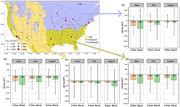
Figure 2. Selected cities of various sizes for the study (A), drought resistance of vegetation growth ( ) for urban and rural areas in June, July, and August, respectively, over the CONUS (B) and in arid, temperate, and continental climate regions (C)–(E) according to Köppen-Geiger climate scheme. City boundaries were delineated using the City Clustering Algorithm applied to MODIS land cover data between 2001 and 2018.
  was computed as the difference in EVI anomalies (
 ) between drought and non-drought conditions. Thus, a less negative value in
  means a stronger ability to resist dampening effects of drought on vegetation growth. Statistical distributions of
  for urban and rural areas individually under drought and non-drought conditions in June, July, and August can be found in figure S4. The EVI data used for the analysis were obtained from the MODIS EVI version 6 product from 2001 to 2018. The mean differences in
  between urban and rural areas in each month are statistically significant (p-value < 0.05) based on t-test applied to data shown in figures S4(B), (C), and (D), except for difference in
  in June between urban and rural areas from the arid region. The vertical line shows the range between minimum and maximum.
Download figure:
Standard image High-resolution image2. Data and methods
2.1. Data for vegetation, weather, and drought
The monthly MODIS EVI Version 6 (MOD13 A3; https://lpdaac.usgs.gov/products/mod13a3v006/) data at 1 km were used as a proxy for vegetation growth and productivity. We only analyzed EVI derived during the growing season, i.e. JJA, between 2001 and 2018, because of the high-water demand from vegetation partly attributed to higher temperatures in summer relative to other seasons. The EVI product is computed from surface reflectance that has been corrected for molecular scattering, ozone absorption, and aerosols. The EVI data are considered a better indicator than normalized difference vegetation index to characterize vegetation status in urban areas since EVI has improved sensitivity in high biomass regions and is less sensitive to canopy background signal and atmospheric influences (Huete et al 2002). In this study, urban extent and its rural counterpart each has a total of 54 observations, i.e. 18 (years) * 3 (months). Urban and rural extents were delineated using the yearly MODIS Land Cover Type (MCD12Q1; https://lpdaac.usgs.gov/products/mcd12q1v006/) Version 6 product (Sulla-Menashe et al 2019) (see details in supplementary document, Section-Delineation of urban and rural extents).
Gridded daily weather data are from the Daymet Version 4 product (Thornton et al
2020) (available at ORNL DACC https://https://daac.ornl.gov/cgi-bin/dsviewer.pl?ds_id=1840), including minimum temperature (Tmin), maximum temperature (Tmax), precipitation (Prcp), shortwave radiation (srad), and day length (dayl) at a spatial resolution of 1 km. The product is derived from daily meteorological observations recorded at weather stations in the North America and has undergone strict cross-validation and quality controls (Thornton et al
2021). srad and dayl were summarized into one variable as daily total radiation (Srad =srad * dayl). The daily weather variables were aggregated to monthly mean values from JJA between 2001 and 2018. Monthly PDSI dataset (Dai 2021) from the National Center for Atmospheric Research Climate Data Guide (https://climatedataguide.ucar.edu/climate-data/palmer-drought-severity-index-pdsi) is used to define dry to wet conditions for each urban-rural pair. PDSI is computed based on information associated with antecedent and current moisture supply (i.e. precipitation) and demand (i.e. potentiation evapotranspiration as a function of air temperature). It is a standardized metric with values typically ranging from −4 to 4 though further extreme values may be possible. The gridded product has a spatial resolution of 2.5 and thus each single urban-rural pair share one PDSI value. The single PDSI value can help understand the background drought conditions. We followed the NOAA Climate Prediction Center (www.cpc.ncep.noaa.gov/products/monitoring_and_data/drought.shtml) to define the drought conditions based on PDSI. Here a PDSI value less than −2 means that urban-rural pairs experience a drought condition and a value larger than 0 but less than 2 means that urban-rural pairs undergo a non-drought condition.
2.2. Drought response of vegetation growth and productivity
Prior to the quantification of drought response of vegetation growth and productivity, common PFTs were identified (further details related to identification of common PFTs can be found in supplementary section 2). Albeit the isolation of common PFTs within urban-rural pairs, EVI signals at 1 km still suffer background spectral contaminations from impervious surfaces or other non-vegetation pixels, resulting in smaller EVI values in urban extents compared to those in rural areas (Zhao et al 2016) with exceptions for urban-rural pairs in semi-arid and arid regions (Georgescu et al 2011) (figure S3). In addition, urban-rural differences in background climate can exert an impact on vegetation growth (i.e. EVI values).
Thus, direct comparisons in EVI between urban and rural areas (e.g. urban EVI minus rural EVI) under drought conditions (PDSI < −2) cannot facilitate revealing differences in drought response of vegetation growth and productivity between urban and rural areas. Here, a linear mixed-effects model was used to help define drought response of vegetation growth and productivity since the model did not have a strong requirement for data distribution (i.e. independent variables may not be necessarily normally distributed, Schielzeth et al (2020)). First, we conducted a panel analysis to remove variation in EVI induced by weather variables including Tmin, Tmax, Prcp, and Srad using equation (1) for all urban and all rural areas individually (thus urban-rural difference in climate variables can be accounted for):
where  refers to EVI observations for city i in month t (June, July, or August) between 2001 and 2018,
  captures the EVI trend over the study period among cities,
  defines the sensitivity of EVI to Tmin, Tmax, Srad, and Prcp, respectively,
  accounts for the random effect without intercept among cities (each city as a group), and
  is the error term. The component
  can account for variations that do not change with climate variables, e.g. variations in EVI attributed to spatial variations of soil quality and impervious surface fractions among different cities and rural counterparts, respectively. Although each urban-rural pair shares one PDSI value extracted from the monthly PDSI dataset, there may be still differences in drought conditions between urban and rural regions. The weather variables including Tmin, Tmax, and Precp in equation (1) can help account for such differences in drought conditions between urban and rural regions that may not be captured by the monthly PDSI dataset. Baseline models without weather variables or random effects were also tested; however, both Akaike information criterion and Bayesian information criterion values pointed to a better model as shown in equation (1).
In general, the grouped regression fitting through equation (1) provides a means to remove climate induced variation in EVI for each urban-rural pair and the model fitted values provided by  terms are assumed as climatologically mean EVI values. Then, we define the difference between original EVI observations and climatologically mean EVI values (i.e. original minus mean) as EVIa (figure 1 shows the flowchart deriving EVIa). Thus, the drought resistance/response of vegetation growth and productivity (represented as Δxa
) is defined using equation (2)
terms are assumed as climatologically mean EVI values. Then, we define the difference between original EVI observations and climatologically mean EVI values (i.e. original minus mean) as EVIa (figure 1 shows the flowchart deriving EVIa). Thus, the drought resistance/response of vegetation growth and productivity (represented as Δxa
) is defined using equation (2)

where x is EVI,  refers to EVIa under drought conditions (PDSI < −2),
  stands for EVIa under non-drought conditions (0 < PDSI < 2), and l represent either urban or rural landscapes.
With equation (2), any city-specific effects such as soil quality and impervious fractions on vegetation status can be largely removed, which provides more confidence in comparing vegetation growth and productivity among the selected 75 cities. Equation (2) was applied to urban and rural extents separately (75*2*3 = 450 times). Droughts are expected to lower the vegetation productivity, and thus  would be negative. A smaller reduction of EVIa during major drought periods suggests a greater resistance of vegetation to the drought impact.
2.3. Urban-rural differences in environmental variables
To help explain the observed discrepancies in drought response of vegetation growth and productivity between urban and rural areas, variables associated with CO2 and O3 concentrations and mean temperature (Tm) were used. The mean temperatures for urban and rural extents individually were computed using Tmin and Tmax provided by the gridded Daymet product following equation (3):

where l refers to either urban or rural extents. CO2 concentrations within urban and rural extents were derived from the bias-corrected column-average dry air mole fraction of CO2 ( ) from Orbiting Carbon Observatory (Eldering et al
2017) (OCO-2, spatial resolution 1.3*2.25 km2). The
) from Orbiting Carbon Observatory (Eldering et al
2017) (OCO-2, spatial resolution 1.3*2.25 km2). The  dataset was obtained from the reprocessed OCO-2 Lite files Version 10 r (available at https://disc.gsfc.nasa.gov/datasets) and has a retrieval accuracy of approximately 1 ppm. Although
  is not a direct measurement of surface CO2 concentration, the
  dataset well characterizes the urban CO2 dome (if any) at the city level (Kort et al
2012, Fu et al
2019) and urban-rural gradients in
dataset well characterizes the urban CO2 dome (if any) at the city level (Kort et al
2012, Fu et al
2019) and urban-rural gradients in  have a linear relationship with surface CO2 gradients (Wang et al
2019). Since the dataset is only available from 2014 and has large gaps in both spatial and temporal domains, the mean
have a linear relationship with surface CO2 gradients (Wang et al
2019). Since the dataset is only available from 2014 and has large gaps in both spatial and temporal domains, the mean  values were computed for urban and rural extents individually using all observations available within the urban or rural extents (i.e.
  values between 2015 and 2019). Thus, we did not further differentiate variation in urban-rural
  gradients among JJA.
The ozone data were obtained using the hourly EPA's Air Quality Data (www.epa.gov/outdoor-air-quality-data) collected at outdoor monitors across the United States. Hourly O3 data from each station within either an urban or rural polygon were aggregated to a monthly scale and then further averaged over all stations within that region (urban or rural). However, only around one-third of urban-rural pairs (24 of 75 urban-rural pairs) had valid monthly mean O3 observations from 2001 to 2018, resulting in large data gaps for analysis. Thus, daily L2 total column O3 data between 2004 and 2018 derived from the Ozone Monitoring Instrument (OMI) (Dobber et al
2006) onboard the Aura satellite (available at https://disc.gsfc.nasa.gov/datasets) were also used to facilitate surface-level O3 estimations. The satellite based O3 data were gridded at 0.25 by 0.25
 and retrieved using the enhanced TOMS version-8 algorithm applied to the ultraviolet radiance data at 317.5 and 331.2 nm with a bias less than 3% (Balis et al
2007). We did not use the satellite based O3 data directly for analysis in this study since the satellite O3 dataset contained the total ozone column data. A regression analysis suggested that there was a statistically significant linear relationship between urban-rural differences in total column O3 and surface O3 gradients (equation (4)) (based on 24 urban-rural pairs, as shown in figure S5(C), with all three months of data considered). Thus, the regression equation was used to convert satellite based monthly mean O3 differences between urban and rural areas to surface urban-rural differences in O3. Behind this conversion, it was assumed that O3 concentration was relatively stable over years for each month (either from satellite- or station-based observations). This assumption was evidenced by figures S5(A) and (B) showing that the ratio between standard deviation and mean of the O3 concentration was relatively small (2%–10%) over years for each month within urban or rural extents.
and retrieved using the enhanced TOMS version-8 algorithm applied to the ultraviolet radiance data at 317.5 and 331.2 nm with a bias less than 3% (Balis et al
2007). We did not use the satellite based O3 data directly for analysis in this study since the satellite O3 dataset contained the total ozone column data. A regression analysis suggested that there was a statistically significant linear relationship between urban-rural differences in total column O3 and surface O3 gradients (equation (4)) (based on 24 urban-rural pairs, as shown in figure S5(C), with all three months of data considered). Thus, the regression equation was used to convert satellite based monthly mean O3 differences between urban and rural areas to surface urban-rural differences in O3. Behind this conversion, it was assumed that O3 concentration was relatively stable over years for each month (either from satellite- or station-based observations). This assumption was evidenced by figures S5(A) and (B) showing that the ratio between standard deviation and mean of the O3 concentration was relatively small (2%–10%) over years for each month within urban or rural extents.
The urban-rural differences in environmental variables (ΔE) including Tm,  (CO2), and O3 were calculated using equation (4):

where E indicates the variable Tm,  , or O3,
  is the mean value in the urban extent, and
  refers to the mean value in the rural region. To determine the main factors in controlling differences in drought response of vegetation growth and productivity, the partial correlations of
  with latitude, longitude, urban size, mean monthly temperature, ΔTm,
  , and ΔO3 were computed. We binned urban-rural differences in Tm,
  and O3 every 0.1
  , 0.1 ppm, and 0.1 ppbv to reduce stochastic error and data uncertainties. ΔT, ΔCO2, ΔO3 were also binned every 0.5
  , 0.5 ppm, and 0.5 ppbv; however, the new binning strategy would not change the significant linear slopes as shown in figures 4(A)–(C).
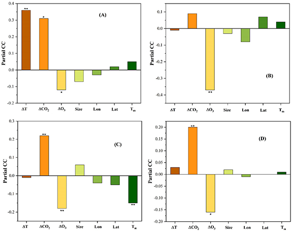
Figure 3. The partial correlation coefficient (Partial CC) of urban-rural differences in drought resistance of vegetation growth ( ) with variables, including urban-rural differences in mean monthly temperature (ΔT), CO2 (ΔCO2), and O3 (ΔO3), city size (Size), longitude (Lon) and latitude (Lat) of a city, and background monthly mean temperature (Tm). ** refers to a statistically significant correlation coefficient at p-value < 0.01 and * for p-value < 0.05. Significance was determined using Student's t-test. (A) CONUS, (B) arid climate, (C) temperate climate, and (D) continental climate.
Download figure:
Standard image High-resolution image
Figure 4. The relationship between urban-rural differences in drought resistance of vegetation growth ( ) and main controlling factors, i.e. ΔT, ΔCO2, ΔO3 (A)–(C), identified over the CONUS. ΔT, ΔCO2, ΔO3 were binned every 0.1
  , 0.1 ppm, and 0.1 ppbv. The solid line refers to a statistically significant slope and the shaded area shows the 95% confidence intervals. The number of samples (
 in three months from 75 cities) before binning is 840 (for ΔT and ΔO3) and each dot in the scatter plots represents a bin. ΔCO2 was computed based on
  averaged between 2014 and 2018 for urban and rural extents individually due to data gaps in both spatial and temporal domains. Thus, the number of samples for ΔCO2 is smaller than those of ΔT and ΔO3.
Download figure:
Standard image High-resolution image
3. Results
Drought resistance of vegetation growth and productivity in urban areas was stronger than drought resistance in rural areas based on analysis of monthly EVI from 2001 to 2018 (figure 2). Statistically significant differences (p-value < 0.05) were observed in  between urban and rural areas except for urban-rural pairs in early summer in arid climate (figure 2). For all selected urban-rural pairs, on average,
  in urban areas, was less negative than that in rural areas regardless of months within the growing season (JJA) (figure 2(B)). These negative
  values are expected since
  refers to the difference in
  between drought and non-drought conditions and mean
  under drought is smaller than that under non-drought conditions (figure S4(B)). A less negative value in
  suggests a stronger ability to resist dampening effects of drought on vegetation growth. More specifically, mean
  in urban areas was −0.0435, −0.0261, and −0.0174, and in rural areas, was −0.0779, −0.0535, and −0.0316, for JJA, respectively (figure 2(B)). Intuitively, it may be reasonable to assume that the less negative mean
  value in urban areas stems from the fact that urban areas typically, except those in arid climate, exhibited a smaller EVI compared to rural regions in each month (JJA) (figure S3). The observed smaller EVI in urban areas in temperate and continental climate zones partly results from the coarse resolution of vegetated pixels (1 km) that suffer signal contaminations from underlying impervious surfaces (i.e. dampening effect of impervious surfaces on EVI). This mixed signal effects (or spectral mixture of vegetation and impervious surfaces within a pixel) can further propagate to
  and
and  calculations, causing smaller standard deviations in
  (figure S4) and
  in urban regions compared to rural regions (figure 2). However, such an intuitive explanation should not be a concern since the
  was computed as the difference in
  between drought and non-drought conditions for urban and rural extents individually (see the section 2 for further details), i.e. we did not compare
  under drought conditions in urban areas with
  under drought conditions in rural areas directly.
As regional climate largely controls the types of ecosystems, we further grouped urban-rural pairs into three main climate zones based on Köppen-Geiger scheme (Beck et al
2018), including arid, temperate, and continental climates. The drought resistance of vegetation growth within each climate zone is shown in figures 2(C)–(E). The separate analysis among climate zones and months shows consistent findings that urban vegetation exhibits stronger ability to resist drought impacts than rural vegetation though the urban-rural differences in vegetation drought resistance varies (figures 2(C)–(E)). In the arid zone, on average,  (urban-rural differences in drought resistance of vegetation growth) was 0.0047 and 0.0135 for July and August (p-value < 0.01), respectively while there was no difference in
  for June (p-value > 0.01). Compared to the arid zone, the temperate and continental climate zones in general showed a much higher value for
  in June and July. For example, the mean
  in July for urban-rural pairs under the continental climate was 0.0133 and under the temperate climate was 0.0177, much higher than 0.0047 for urban-rural pairs from the arid zone. For mean
  in August, urban-rural pairs from the temperate zone exhibited the largest value (0.0148), followed by those from the arid (0.0135) and continental (0.017) climate zones.
We next explored the potential effects of several drivers underlying urban-rural discrepancies in drought resistance of vegetation growth, including urban-rural differences in monthly mean temperature (ΔT), CO2 (ΔCO2), and O3 (ΔO3), city size (Size), the latitude and longitude of a city (Lat and Lon, in case spatial location would be a factor), and background monthly mean temperature (Tm). To find the main factors controlling  , partial correlation coefficients (partial CC) between
  and potential drivers were computed for all selected urban-rural pairs from all three climate zones (figure 3(A)) as well as separately for arid (figure 3(B)), temperate (figure 3(C)), and continental climates (figure 3(D)). The main factors in controlling
  across the conterminous U.S. were ΔT (partial CC of 0.36), ΔCO2 (0.31), and ΔO3 (−0.12) as seen in figure 3(A). Significant linear relations were also observed for the associations of ΔT, ΔCO2, ΔO3 and
  from binned observations (figure 4) that were adopted to reduce stochastic error and data uncertainties in the analysis. The main controlling factors for
  in each climate zone were different among three climate backgrounds. For example, the most influential variable was ΔO3 in the arid zone (partial CC of 0.37, figure 3(B)), while in the temperate zone, the main drivers influencing
  were ΔCO2 (partial CC of 0.22), ΔO3 (partial CC of −0.18), and Tm (partial CC of −0.15) (figure 3(C)). In the continental zone (figure 3(D)), ΔCO2, followed by ΔO3 was the main factor in affecting
  . Overall, ΔT was identified as a main driver for
  over the CONUS but not in each climate zone. Further explanations for this finding were presented in the discussion section.
4. Discussion and conclusions
We found urban ecosystems were more resistant to drought compared to their rural counterparts regardless of climate zones across CONUS. However, the main variables that contribute to such urban-rural differences in drought resistance of vegetation growth varies among climate zones. In general, surface temperature gradient (ΔT) was the most influential factor (p-value < 0.01, figure 2(A)) at the continental scale that consists of various ecosystems. Higher temperature in urban areas in relative to rural areas, observed for most of the selected urban-rural pairs (figure S6), likely leads to an earlier start but later end of the growing season and thus a longer growing season (Li et al
2017, Wang et al
2019), resulting in enhanced vegetation growth prevalent in urban areas (Zhao et al
2016) (while still a lower EVI value compared to rural areas due to the dampening effect from impervious surfaces). Thus, when the very same drought occurred in both urban and rural areas, the enhanced vegetation growth attributed to higher temperatures in urban areas exhibited a better ability/chance to endure/survive drought stress. In addition, plants growing in warmer/drier urban environments may already have had (screened before planting) or developed traits that allow them to better cope with drought stress (Anderegg and HilleRisLambers 2016). However, ΔT was not the controlling factor driving the urban-rural contrast of vegetation drought resistance within individual climate zones as shown in figure 3 partly due to the much less variation of ΔT in each climate zone (figure S7). Specifically, as shown in figure S7, vegetation growth in arid or semi-arid cities in general exhibits a much stronger drought resistance compared to that in the other two climate zones despite a wide range of ΔT from −2.0 °C to 3.5  . Even though urban-rural difference in drought resistance varies from −0.10 to 0.11 within temperate or continental climate regions, in a similar magnitude of variation in arid climate, there is a much smaller variation of ΔT. Thus, the urban-rural temperature gradient is not strong enough to cause such considerable differences in vegetation growth. The stronger drought resistance of vegetation (mainly shrub and grass) growth in cities from the arid zone was mainly related to vegetation growth in rural areas exposed to higher ozone concentration (figure S8). Higher ozone concentration in rural areas than in cities (Gregg et al
2003), could cause more reduction in photosynthesis and vegetation growth in rural areas (Ainsworth et al
2012), which accounted for the negative relationship between surface O3 gradients and urban-rural differences in drought resistance of vegetation growth (figures 3 and 4(C)). In addition, urban-rural difference in drought resistance of vegetation growth in the temperate zone is also sensitive to background monthly mean temperature Tm. Since the selected urban-rural pairs from the temperate climate zone exhibits the highest background monthly mean temperature (figure S9), this result emphasizes possible temperature stress on vegetation growth, particularly in urban areas, given relatively stable temperature gradients for urban-rural pairs from the temperate zone (figure S7).
. Even though urban-rural difference in drought resistance varies from −0.10 to 0.11 within temperate or continental climate regions, in a similar magnitude of variation in arid climate, there is a much smaller variation of ΔT. Thus, the urban-rural temperature gradient is not strong enough to cause such considerable differences in vegetation growth. The stronger drought resistance of vegetation (mainly shrub and grass) growth in cities from the arid zone was mainly related to vegetation growth in rural areas exposed to higher ozone concentration (figure S8). Higher ozone concentration in rural areas than in cities (Gregg et al
2003), could cause more reduction in photosynthesis and vegetation growth in rural areas (Ainsworth et al
2012), which accounted for the negative relationship between surface O3 gradients and urban-rural differences in drought resistance of vegetation growth (figures 3 and 4(C)). In addition, urban-rural difference in drought resistance of vegetation growth in the temperate zone is also sensitive to background monthly mean temperature Tm. Since the selected urban-rural pairs from the temperate climate zone exhibits the highest background monthly mean temperature (figure S9), this result emphasizes possible temperature stress on vegetation growth, particularly in urban areas, given relatively stable temperature gradients for urban-rural pairs from the temperate zone (figure S7).
Surface CO2 gradient is identified as another important factor, in addition to surface temperature and O3 gradients, responsible for the observed urban-rural discrepancies in drought resistance of vegetation growth. The surface CO2 gradient is represented by the satellite-based  gradient since there is a positive, linear relationship between the two (with a scale factor of ∼25) (Wang et al
2019). This satellite-based CO2 gradient dataset (figure S10) shows that a greater difference in CO2 concentration between urban and rural areas could result in a much stronger urban-rural difference in drought resistance of vegetation growth, particularly under temperate and continental climates (figures 3(A), (C), (D) and 4(B)). This conclusion is consistent with previous studies that emphasize the beneficial effect of atmospheric CO2 enhancement on vegetation growth under drought conditions by stimulating photosynthesis (Ainsworth and Rogers 2007) or by increasing the water use efficiency of plants (Keenan et al
2013). However, the beneficial effect of CO2 on urban-rural contrast in drought resistance is observed in temperate and continental zones rather than in arid zones even though urban-rural pairs from the arid zone typically showed the largest CO2 gradient (figure S11). The insensitivity of drought impact on vegetation growth to CO2 gradients in the arid zone, relative to other two climate zones, may result from other more limiting factors such as nutrient deficiency (Wang et al
2020) or stomatal closure in response to rising CO2 at the cost of enhanced growth (Frank et al
2015) in urban regions from the arid zone. Drought in the water-limited region is often more severe (as indicated in figure S12), and it is also possible that such drought condition completely overwhelms the beneficial effects of elevated CO2 on vegetation growth.
gradient since there is a positive, linear relationship between the two (with a scale factor of ∼25) (Wang et al
2019). This satellite-based CO2 gradient dataset (figure S10) shows that a greater difference in CO2 concentration between urban and rural areas could result in a much stronger urban-rural difference in drought resistance of vegetation growth, particularly under temperate and continental climates (figures 3(A), (C), (D) and 4(B)). This conclusion is consistent with previous studies that emphasize the beneficial effect of atmospheric CO2 enhancement on vegetation growth under drought conditions by stimulating photosynthesis (Ainsworth and Rogers 2007) or by increasing the water use efficiency of plants (Keenan et al
2013). However, the beneficial effect of CO2 on urban-rural contrast in drought resistance is observed in temperate and continental zones rather than in arid zones even though urban-rural pairs from the arid zone typically showed the largest CO2 gradient (figure S11). The insensitivity of drought impact on vegetation growth to CO2 gradients in the arid zone, relative to other two climate zones, may result from other more limiting factors such as nutrient deficiency (Wang et al
2020) or stomatal closure in response to rising CO2 at the cost of enhanced growth (Frank et al
2015) in urban regions from the arid zone. Drought in the water-limited region is often more severe (as indicated in figure S12), and it is also possible that such drought condition completely overwhelms the beneficial effects of elevated CO2 on vegetation growth.
Despite the identified main variables, factors such as landscape configuration/composition, atmospheric deposition (e.g. nitrogen and phosphorus), and management practices may also affect the observed discrepancies in drought resistance of vegetation growth between urban and rural areas. For example, urban landscape configuration and composition has been related to surface temperature gradients between urban and rural areas (Connors et al 2013, Estoque et al 2017), thus either strengthening or accentuating the effect of temperature gradients on difference in drought resistance between urban and rural vegetation growth. As urban areas typically have a higher atmospheric nitrogen and phosphorus deposition (Decina et al 2018), this may lessen nutrient restrictions on vegetation growth, thus contributing positively to the observed differences in drought resistance of vegetation growth between urban and rural areas. Human practices such as urban irrigation, however, may be a factor weakening the conclusion made towards the main factors driving the urban-rural differences in drought resistance of vegetation growth. Thus, we repeated the analysis by excluding some urban-rural pairs from the arid zone where irrigation typically was most pronounced and led to 'the oasis effect' (Georgescu et al 2011), i.e. higher EVI in cities than in rural areas (figure S3). Further analysis of urban-rural pairs from the three climate zones suggests that the main factors controlling the urban-rural differences in drought resistance of vegetation growth are still gradients of temperature and CO2 and O3 concentrations but with a smaller partial CC (figures S13 and 3(A)). Thus, although urban irrigation contributed positively to the observed urban-rural contrasts in drought resistance of vegetation growth, such a factor alone could not explain all the observed variances associated with drought resistance. Even under strong irrigation for cities in the arid zone, surface O3 gradient was still identified as the main driver for observed discrepancies in drought resistance of vegetation growth between urban and rural areas (figure 3(B)). As such, there is strong evidence in attributing the observed discrepancies in drought resistance of vegetation growth between urban and rural areas to factors including temperature, CO2, and O3 gradients. Urban-rural gradients in wind speed and humidity were also accounted for in the analysis (figure S15). The results suggested the controlling factor for the urban-rural differences in drought resistance would still be temperature, CO2, and O3 gradients (figure S15).
Benefiting from long-term satellite and station-based datasets, our study provides a data driven approach for revealing the impacts of competing and interactive environmental factors on response of vegetation growth to drought at a large scale. This approach advocates the urban plant physiology concept by utilizing urban-rural contrasts in environmental conditions, such as altered temperature gradients and O3 concentration. The substantial differences in environmental conditions along urban-rural gradients can provide a 'natural laboratory' that is more widely accessible, compared to manipulative environments, to the scientific community to understand ecosystem traits under a changing climate. With projected increase in temperature and atmospheric CO2 in the future, we can also select only urban-rural pairs with positive values in ΔT and ΔCO2 for analysis. In this case, it is found that the mean urban-rural difference in drought resistance of vegetation growth becomes positive, i.e. 0.0389 for June, 0.0294 for July, and 0.0201 for August (figure S14). Thus, the novel aspect of this study is to provide a more general assessment of vegetation responses to environmental factors across different regions, and ultimately, to reduce uncertainties in quantifying terrestrial carbon dynamics.
Acknowledgments
Fu and Bernacchi would like to acknowledge the funding support from Global Change and Photosynthesis Research Unit of the USDA Agricultural Research Service. Hu is partly funded by NASA Projects (80NSSC20K1263 and 80NSSC21K0430). Any opinions, findings, and conclusions or recommendations expressed in this publication are those of the author(s) and do not necessarily reflect the views of the USDA. Mention of trade names or commercial products in this publication is solely for the purpose of providing specific information and does not imply recommendation or endorsement by the U.S. Department of Agriculture. USDA is an equal opportunity provider and employer. We would like to thank Jesse McGrath for writing R scripts in accessing US EPA Air Quality Data. We are also grateful to editors and three anonymous reviewers for their thought comments and suggestions which helped improve this manuscript.
Data availability statement
All data that support the findings of this study are included within the article (and any supplementary files).
Conflict of interest
The authors declare no conflicts of interest relevant to this study.