Contamination Event Detection Method Using Multi-Stations Temporal-Spatial Information Based on Bayesian Network in Water Distribution Systems

Abstract

As a core part of protecting water quality safety in water distribution systems, contamination event detection requires high accuracy. Previously, temporal analysis-based methods for single sensor stations have shown limited performance as they fail to consider spatial information. Besides, abundant historical data from multiple stations are still underexploited in causal relationship modelling. In this paper, a contamination event detection method is proposed, in which both temporal and spatial information from multi-stations in water distribution systems are used. The causal relationship between upstream and downstream stations is modelled by Bayesian Network, using the historical water quality data and hydraulic data. Then, the spatial abnormal probability for one station is obtained by comparing its current causal relationship with the established model. Meanwhile, temporal abnormal probability is obtained by conventional methods, such as an Autoregressive (AR) or threshold model for the same station. The integrated probability that is calculated employed temporal and spatial probabilities using Logistic Regression to determine the final detection result. The proposed method is tested over two networks and its detection performance is evaluated against results obtained from traditional methods using only temporal analysis. Results indicate that the proposed method shows higher accuracy due to its increased information from both temporal and spatial dimensions.

1. Introduction

Water distribution systems (WDSs) are of indispensable significance for city water supply, especially considering that their safety directly affects public health. However, during the long delivery process from water plant to users, the water quality in WDSs deteriorates because of the effects of the distance and time taken. Additionally, it is vulnerable to external disturbances, such as sabotage, because of its openness. For these reasons, contamination event detection for water quality is crucial in early warning systems of WDSs.

In previous methods of water quality event detection, hydraulic model, and water quality balance model are used to simulate the changes in water quality; including the QUAL model [1], BASIN model [2], and Mike model [3]. For WDSs, dispersion and effect analysis of specific substances or organisms are focused in some methods of contamination event detection. Hall and Szabo [4] studied the effects of common contaminants on the water quality index of drinking water, including herbicide (glyphosate), insecticide (aldicarb), alkaloid (nicotine), and industrial raw materials (arsenic, and potassium ferricyanide). The corresponding relation was given between the concentration of the contaminants and variation of water quality index quantitatively in their paper. Jeffrey et al. [5] modelled the diffusion of common contaminants, such as herbicide, insecticide, colibacillus, and biological medium in water pipes. With the rapid development of computer science, the data mining methods became increasingly concerned by researchers. The use of these methods means that large amounts of data from the water quality’s monitoring system can be used to analyse changes in water quality, which reduces the modelling complexity of real systems. Byer and Carlson [6] proposed a method that used the differences between values of background data and detection data to detect events. However, background data is susceptible to baseline drift and background noise. In effort to resolve this problem, many researchers endeavoured to represent the background data as much precision as possible. Mckenna et al. [7] used the Time Series Increment (TSI) model and the Autoregressive (AR) model in event detection to show background fluctuation. Arad et al. [8] developed a detection method where the threshold was updated in two stages: in-line and on-line. In the first stage, five decision variables were tuned and in the second stage the five decision variables were used for real-time and on-line event detection. Liu et al. [9] presented a detection method based on time-frequency analysis. The Hilbert-Huang Transformation was used to decompose the time sequence of water quality data into a series of Intrinsic Mode Functions, in order to avoid nonlinear and non-stationary fluctuation in background data. Additionally, some machine learning algorithms have been used in water quality contamination event detection. Klise [10] introduced a detection method that combined the K-means cluster and K Nearest Neighbor (KNN) classification algorithm. Vugrin et al. [11] distinguished events from the fluctuation caused by working conditions by using trajectory cluster through feature extraction and cluster using fitting polynomial of data. Modaresi and Araghinejad [12] evaluated three methods: Support Vector Machine, Probabilistic Neural Network, and KNN of water quality event detection, and compared their performance.

WDSs consist of numerous stations, with the characteristic of large scale and high complexity. This means that event detection in WDSs always works with real-time data and information from multiple stations, rather than single station. More researchers have focused on detection with multiple stations. O’Halloran et al. [13] demonstrated in field trials that parameter fluctuations were partially preserved for significant periods of time and they suggested a water parcel tracking technique for characterising the connectivity between sensors. Koch and Mckenna [14] analysed clusters using spatial data from water quality sensors and improved early warning and traceability analysis with data fusion technology using both geographical positions and temporal information. In their research, KNN was used for the analysis of neighbor nodes information, including water quality data and the sensors’ situation. Mao et al. [15] examined the methods that are used in wireless sensor networks. The Bayesian Network was used for the spatial detection of a river’s network and Markov chain for the temporal detection to improve the performance of the detection. Oliker and Ostfeld [16] improved the performance of event detection by using a model that incorporates hydraulic simulation information into the overall event detection process of spatially distributed sensors, resulting in a decrease of false alarms. Stoianov et al. [17] developed a method for the network construction of water quality event detection and also analysed the relationship between different nodes and water quality variables based on the frequency-domain analysis method. However, in these methods, spatial analysis is often regarded as a supplementary consideration following time analysis. The fusion methods for spatial and temporal information are often cascaded and unsupervised. There is also a variety of historical information that is seldom used in the multi-stations detection method for causal relationship construction.

As has been noted, due to the distinctive structure of WDSs, there is also a relationship between water quality data from a downstream station and its upstream stations. The direction of the water’s flow and its transitivity lead to a causal relationship between the upstream stations and the downstream stations. To date, the local information of a single station is isolated from other stations in a network, which leads to a limitation in accuracy. This paper aims to improve detection performance by developing a contamination event detection method that incorporates not only the temporal information from one single station, but also the spatial information based on causal relationship analysis of that station and its upstream stations. The causal relationship model is simulated by Bayesian Network (BNT), based on topology of the network, hydraulic features of water flow, and historical water quality data, rather than real-time correlation analysis. A supervised learning algorithm, Logistic Regression, is selected to integrate probabilities from the temporal and spatial analysis for that station, in order to derive more accurate results than from an unsupervised method. As the temporal and spatial information are considered simultaneously, with the combined addition and emendation of these two dimensions, accuracy will be improved. Two kinds of methods using only temporal analysis are compared, respectively, with the proposed methods in two different cases for demonstration.

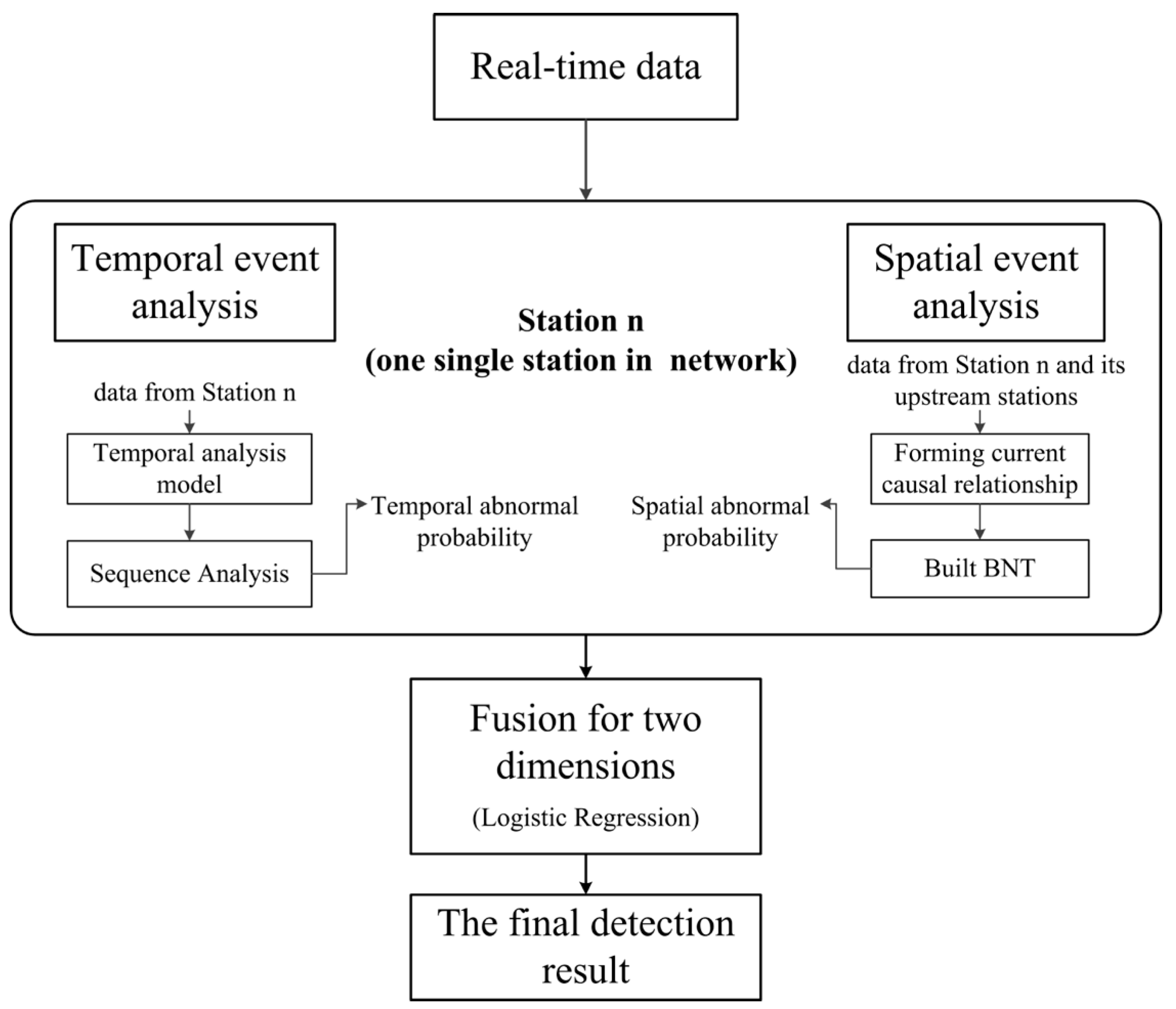
2. Methodology

An integrated method for water contaminant event detection is proposed to combine temporal information from a single station with spatial information from its upstream stations. The temporal abnormal probability of a single station is gained by two kinds of time sequence analysis methods, the threshold model or the AR model, using local water quality data. The spatial probability is derived by comparing the current causal relationship with the conditional probability table of the built causal relationship between that station and its upstream stations. Logistic Regression is used to combine the analysis results from the temporal and spatial analyses, and to decide the final detection result. The design of scheme is shown in Figure 1 and the details of the model will be described in the following sections.

2.1. Temporal Event Analysis Based on Local Information

The Threshold Model and AR Model

In the threshold model, a dynamic threshold is obtained by using historical data to decrease the effect of fluctuations and cyclical change in water quality data. A sliding window is used to separate the time sequence of water quality data into different parts, so that, the threshold is not the same in relation to its different situation in the time sequence. Suppose that the length of the sliding window is L, and the mean value of the time sequence of background data with the length of L is $\overline{d}$, then the standard deviation of it is $\mu$, for the new-in data $x_t$.

According to the three-sigma rule, if

$$|x_t-\overline{d}|>3\mu$$

(1)

then we reckon that $x_t$ is abnormal. Otherwise, it is a normal time step.

The AR model [18,19] is used for parameter prediction and for determining whether a time step is abnormal using prediction residual and threshold, and the Bayesian information criterion (BIC) and least-squares method are implemented for model parameter calibration.

Sequence analysis is used for obtaining temporal abnormal probability for each time step using sequence consisting of several continuous time steps [20] after using the threshold or AR model.

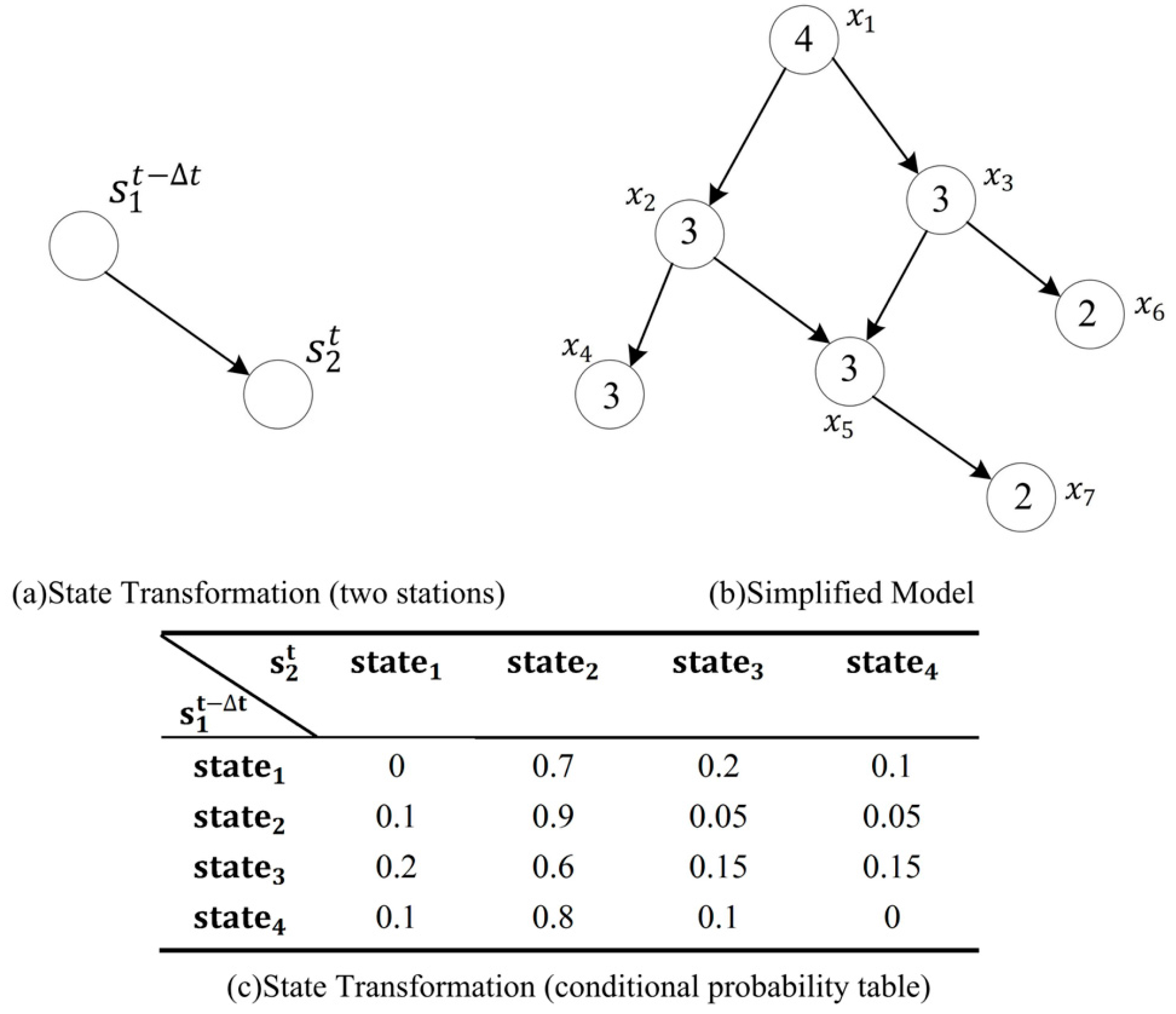
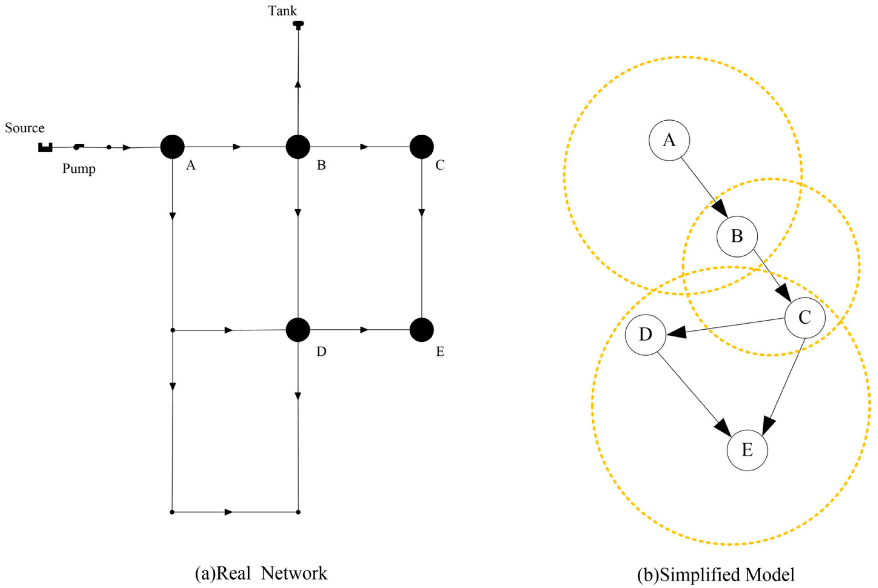
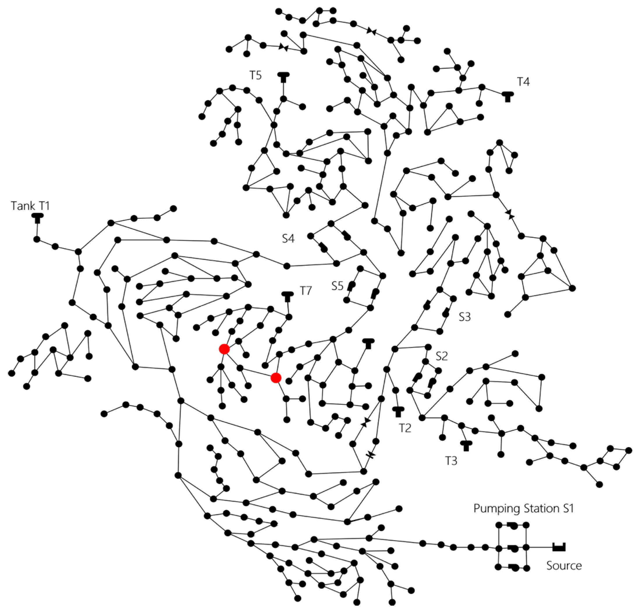
2.2. Spatial Event Analysis Using Causal Relationship Based on Multi-Stations’ Information

The probability graphic model simplifies the complexity of the real world and simulates the uncertainty of data. Using probability to describe the causal relationship between stations is also convenient for merging with temporal event detection results. The Bayesian Network, which was first proposed in 1985 by Judea Pearl (Parsons [21]), is one of the most frequently used probability graphical model. It is chosen in this paper to simulate the causal relationship between an upstream station and its downstream stations. It consists of two elements: the model structure and its parameters (conditional probability table). Its basic concept is based on the following formula [22]. The joint probability for the assignment of any set of values $x_1$, …, $x_n$ to the set of variables $X_1$, …, $X_n$ in a BNT can be determined by

$$p(x_1,\cdots x_n)={\displaystyle \prod }_{i=1}^{n}P(x_i|Parents(X_i))$$

(2)

where $Parents(X_i)$ is a set of values for the preceding nodes in the network. A critical feature of the Bayesian Network is that after each node is determined by the value of its direct precursor node, this node condition is independent of all its non-direct predecessor nodes. The construction of Bayesian Network is described as follows:

1. Structure forming

The Bayesian Network is a directed acyclic graph $G=\langle V,E\rangle$. V represents the station in network and E is edge connecting stations. The simplified model is shown Figure 2b, where node $x_n$ represents the water quality detection station. Water quality data, such as residual chlorine concentration, pH, and conductivity are taken as random variables at the node.

2. Parameter learning

The causal relationship is generated by the water flow between stations. If the water flow time from an upstream station to its downstream station is $\Delta t$, the influence brought by the upstream station on the water quality will be reflected at its downstream station after $\Delta t$. Thus, the water quality data should be shifted when forming the Bayesian Network. That is to say, the water quality data of an upstream station at t corresponds to the data of its downstream station at $t+\Delta t$. Let the state of station $i$ at time step t be $s_i^t$, $\Delta t_i$ is the water flow time between the two stations. The training data for parameter learning should be an s-tuple $(s_1^{t-{\Delta t}_1},s_2^{t-{\Delta t}_2},\cdots ,s_{n-1}^{t-{\Delta t}_{n-1}},s_n^t)$. The water quality data should be discretised into different states for parameter learning. Maximum likelihood estimate is used to learn the parameters of the Bayesian Network based on historical data.

After the training process, a conditional probability table, such as that in Figure 2c, is obtained to represent the causal relationship between two stations, where $s_1$ represents the state of an upstream station, $s_2$ is the state of its downstream station after $\Delta t$. Figure 2 shows the state transformation between stations and the state transformation for the whole simplified network. Apparently, if there are two upstream stations and four states for each station, the conditional probability table for that station should be a cell of $4\times 4\times 4$.

3. Using Bayesian Network for inference

Suppose that the current state of downstream station is $s_2^t=stat{e}_n$, the water flow time is $\Delta t$ between stations, and the state of the upstream station at $t-\Delta t$ is $s_1^{t-\Delta t}=stat{e}_m$. Based on the conditional probability table, look for the probability $p$ when the upstream state is $stat{e}_m$ and the downstream state is ${state}_n$. The abnormal probability is considered to be $1-p.$ For example, the state of the upstream station is $s_1^{t-\Delta t}={state}_2$, and the downstream station is ${state}_2$. Based on the conditional probability table shown in Figure 2c, the probability of abnormal is (1 − 0.9) = 0.1; if the state of the downstream stations is ${state}_3$ when its upstream station is ${state}_2,$ the abnormal probability of it should be (1 − 0.05) = 0.95.

2.3. Fusion of Abnormal Probabilities from Temporal Dimension and Spatial Dimension

After the above two steps are completed, Logistic Regression is chosen to derive the detection results, as well as the probability. With this supervised classification method, the threshold and the weights of the two dimensions of classification can be obtained using training sets rather than by manual tuning. The abnormal probabilities of a single station for each time step are achieved by both temporal and spatial analysis, using training sets. Taking these two probabilities as two features of one training sample, the time step of real event is labelled with 1 while the normal operation is considered as 0, to classify these samples. The weights of two probabilities are obtained, in order to make the final decision of the proposed method after training. Let $({\mathit{x}}^{(i)},{\mathit{y}}^{(i)})$ represents the $i_{th}$ training sample for a single station in the WDSs for the logistic model, where $\mathit{x}=(x_1, x_2)$, $x_1$ is the abnormal probability from temporal analysis based on local information, and $x_2$ is the abnormal probability from spatial analysis based on that station and its upstream stations. The logistic model is described as follows:

$$P(E=1|x_1, x_2)=\frac{1}{1+e^{-({\theta }_0+\sum {\theta }_i{x}_1)}}$$

(3)

where ${\theta }_i$ is the parameter for the logistic model based on training samples. E = 1 shows that the time step is classified as an event.

The detailed steps are described as follows:

• Find a hypothesis function which is usually simplified as h function;

  $$h_{\theta }(x)=g ({\theta }_0+{\displaystyle \sum }{\theta }_i{x}_1)$$

  (4)

  in which

  $$g(z)=\frac{1}{1+e^{-z}}$$

  (5)
• Construct a Cost Function and it represents the deviation of the hypothesis output from the label y in training sets;

  $$J(\theta )=\frac{1}{m}{\displaystyle \sum }_{i=1}^{m}Cost({h_{\theta }}^{(i)},y^{(i)})$$

  (6)

  $$cost(h_{\theta }(x),y)=\{\begin{array}{cc}-\log (h_{\theta }(x))& if y=1\\ -\log (1-h_{\theta }(x))& if y=0\end{array}$$

  (7)

  where $m$ is the number of training samples.
• Use Gradient Descent to minimise the cost function $J(\theta )$.

3. Application and Experiments

3.1. Data Formation

Still, real events in WDSs are nearly absent. So, the simulation tool, EPANET (Rossman [23]), is used in this section to provide the dataset. Chlorine is one of the most commonly used disinfectants in water treatment and it is taken as the water quality index for evaluation in this paper. To simulate events, chlorine is added to the chosen station as a contaminant. Event properties, such as the start time, length, and strength of the event, as well as the station, we add the contamination to can be set by codes using MATLAB and EPANET. In order to simulate the real situation, noise is also added to the data generated from EPANET because the origin data is too ideal.

3.2. Experimental Procedure

First, the average flow time between stations and the residual chlorine concentration for each station is obtained by simulations. The residual chlorine concentration is represented in term of time sequence. The original time sequence is added with random noise, and then the acquired time sequence and the average flow time will be regarded as historical data for training. They will be used for deriving parameters of the AR model, the threshold model and the conditional probability table of the Bayesian Network. Testing data are obtained by using another set of historical data thereafter superimposing events on them. The proposed method is demonstrated using two different networks and is compared with the method that uses only temporal analysis. The indexes of the performance evaluation chosen here are True Positive Rate (TPR) and False Positive Rate (FPR), which are widely used in performance examination [16].

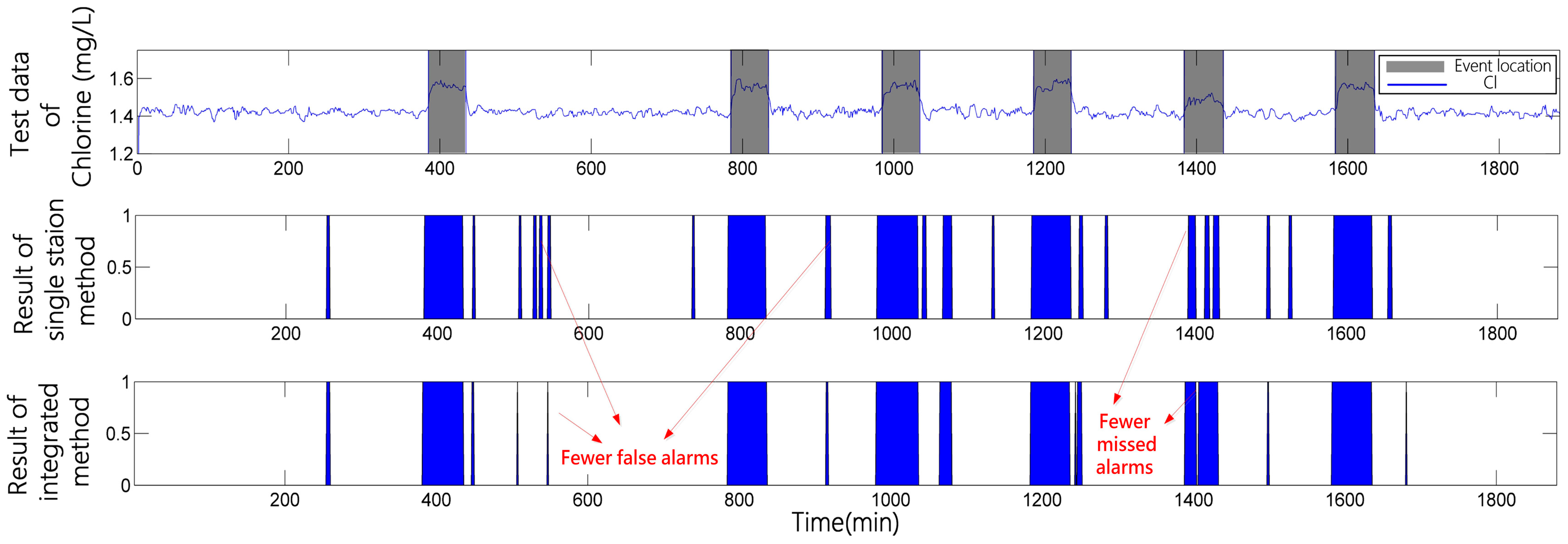
3.3. Experiment and Analysis

3.3.1. Case 1

This network consists of nine nodes, one reservoir, one tank, and one pump (Figure 3a). The labelled nodes are chosen as the monitoring stations. A simplified graphic model consisting of the chosen stations is shown in Figure 3b. The arrows in this figure show the flow direction. The network is maintained in normal operation for two days and sampled every one minute for the residual chlorine concentration to be historical data. In order to build the causal relationship, the Bayesian Network should be trained first.

Forming of the Bayesian Network

Figure 3a shows five stations, marked A–E. Due to the conditional independence of the Bayesian Network, the conditional probability only exists between a node and its parent nodes that connected directly to it. In Figure 3b, A and B are both the upstream stations of station C. But, A and C are not directly connected. When forming the structure, B is the only parent, or upstream station for station C for building causal relationship. The circles in Figure 3b represent the sub-net for each node with its parent nodes. The state of each station is determined by the concentration of chlorine in this paper. For the sake that the concentration level of residual chlorine is different at different stations, the discretisation of concentration is independent for each station. Let the maximum value of the historical data at station n be ${s^n}_{\max }$, and the minimum value be ${s^n}_{\min }$. If the concentration at a time step is less than ${s^n}_{\min }$, the state of this time step is considered to be state 1 and state 2 is for concentration between $[{s^n}_{\min },\frac{{s^n}_{\max }-{s^n}_{\min }}{2})$, state 3 for between $[\frac{{s^n}_{\max }-{s^n}_{\min }}{2},{s^n}_{\max })$, state 4 for more than or equals to ${s^n}_{\max }$.

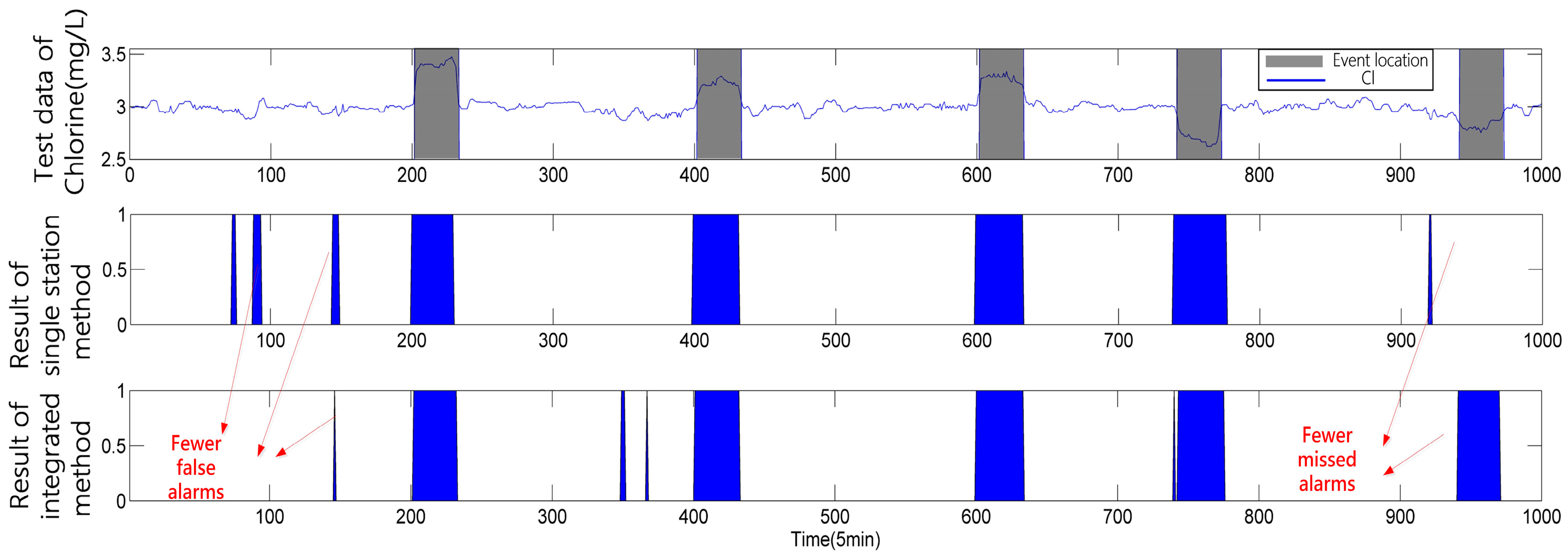
Temporal Analysis Based on Single Station Information

Here, the sub-net that consists of B and C is discussed. In the first step, the threshold model is implemented for temporal analysis using only local information from C. Contamination is injected at station A. Due to the noise in water quality data and the fluctuation of the background, the threshold model performances are not as expected, even when a suitable window is chosen as shown in the second sub-picture of Figure 4. Additionally, the constant length of the window is less helpful to the model’s flexibility for fluctuation with different periods, leading to an increase in false alarms. Using higher thresholds decrease the false alarms, but also decrease the detection rate, and, therefore, it is more difficult to find events with lower concentrations. However, both false alarms and detection rate will increase if we do the opposite, because some fluctuation and noise with similar strength will be taken as events.

Spatial Analysis Using Causal Relationship Based on Multi-Stations Information

In this step, the Bayesian Network is constructed to simulate the causal relationship between one station and its upstream station. The average flow time between upstream and downstream stations is obtained using the hydraulic information from Oliker and Ostfeld [16]. The unit of pattern of EPANET is one hour; the flow velocity and length of pipe are used to derive the time the water takes to flow from one station to its downstream station for each hour. After this, the average time is calculated as the water flow time between stations for building the causal model and for event detection. In this case, the water flow time is 134 min. Then, the causal relationship model can be built based on the water flow time between stations and historical data. Then, integrate its testing results in terms of probability as spatial information with the results from the temporal dimension.

The curve, as shown in the first sub-figure of Figure 4, shows the test data for residual chlorine concentration and the event is marked with a square. The single station method means that the method uses only local information from one single station; the integrated method means that the proposed method uses both local information and spatial information from multiple stations. It can be observed that there are some false alarms and missed alarms in the result of the single station detection. The third sub-figure shows that the result of the proposed integrated method performs better than the single station analysis method. This is because some missed alarms, which are caused by the low concentration of contaminants, are compensated, and some false alarms are calibrated by the process of bringing in information from the spatial dimension. However, the imported information also brings in false alarms. With mutual calibration, false alarms generally decrease. Six experiments are employed to evaluate the proposed method. The results of TPR and FPR are recorded in

Table 1. Performance comparison between the single station method based on the threshold model and the fusion method combining temporal and spatial information (TPR, FPR).

Scenario	Single Station Method		Integrated Method
	TPR	FPR	TPR	FPR
1	0.9233	0.0873	0.9367	0.0310
2	0.8967	0.0342	0.9500	0.0114
3	0.8833	0.0551	0.9333	0.0234
4	0.9333	0.0582	0.9733	0.0222
5	0.8933	0.0658	0.9400	0.0506
6	0.9067	0.0532	0.9700	0.0354
Average	0.9061	0.0590	0.9501	0.0290

. It can be seen that the TPR increase and the FPR decrease, which shows a better performance when compared to the single station method.

3.3.2. Case 2

The structure of this case is shown in Figure 5 and is based on the work of Ostfeld et al. [24]. It has a different size and hydraulic condition when compared to the network of in Case 1. This network consists of 388 nodes, 429 pipes, one reservoir, and seven tanks. The network is kept working for 200 h and the residual chlorine data is measured every five minutes. Nodes 328 and 311 are chosen as monitoring stations, where 328 is the upstream station and 311 is its downstream station. The chosen stations are marked in red in Figure 5.

Temporal Analysis Based on Single Station Information

The AR model is often used for the description of water quality background data, and is sometimes more adaptive to describe the fluctuation in water quality data. In this case, the AR model is chosen to be the single station temporal analysis method. When an event with high concentration is superimposed on the normal operation, there will be a large difference between the predicted value and the measured value. So the event can be found according to the difference. Nevertheless, complex variations of background data can lead to inaccuracy of the AR model. When the concentration of the contaminant decreases, the AR model no longer gives a satisfactory result. The reason for this is that the low-concentration event with similar fluctuation with the background data will be taken as a normal operation in the trained AR model, which results in missed alarms in detection even if the model has been optimised. However, if the trained AR model is sensitive to classify the fluctuation of background and event, this may cause more false alarms. In this case, using the information from upstream stations based on Bayesian Network can help to decrease missed alarms by discovering these types of events, but which may also import false alarms. Hence, a fusion of the two dimensions is needed to perfect performance.

Spatial Analysis Using Causal Relationship Based on Multi-Stations Information

After integrating the informational from spatial analysis with the temporal analysis, the results are shown in Figure 6 and

Table 2. Performance comparison between the single station method based on the AR model and fusion method, combining temporal and spatial information (TPR, FPR).

Scenario	Single Station Method		Integrated Method
	TPR	FPR	TPR	FPR
1	0.9400	0.0556	0.9800	0.0181
2	0.9063	0.0850	0.9500	0.0500
3	0.8400	0.0462	0.9467	0.0145
4	0.8750	0.0946	0.9563	0.0573
5	0.9467	0.0485	0.9533	0.0169
6	0.9125	0.0766	0.9313	0.0207
Average	0.9034	0.0678	0.9529	0.0295

. The figure shows that the last series of event cannot be found by the single station model based on the AR model and sequence analysis, because its fluctuation is similar to the normal background fluctuation in this trained AR model. There are also some false alarms in the result. After the integration process, the missed events can be found. Some new false alarms are brought in by the spatial information but the false alarms are decreased in general by using suitable parameters in the fusion process. Similar to Case 1, six experiments are also employed, which demonstrated the superiority of the proposed method of contamination event detection.

4. Conclusions

In order to use both spatial and temporal information fully, and to improve accuracy in contamination event detection in WDSs, an event detection method is proposed in this paper for the fusion of both temporal and spatial analysis. The proposed method is compared with two temporal analysis detection methods separately in two different networks of different size, for the purpose of evaluation. Performance indicates that our proposed method’s fusion model is better and has a higher accuracy than the threshold model and AR model. The proposed method compensates for the deficiency of the AR model where the AR model that is trained by fluctuant training data cannot distinguish between a low-concentration event and the background fluctuation. As for the threshold model, its inadequate adaptation to background fluctuation and noise, and the subjective threshold value will lead to unsatisfactory results. However, by introducing the information from spatial analysis between stations, the TPR results increase and FPR results decrease. Furthermore, the threshold of the fusion model does not need to be chosen by tests or subjective judgement. By changing the training samples, the model can be better in adapting to different networks. In the fusion process, the two dimensions are considered parallel, which also solves the problem that any mistakes will be amplified in the next stage in cascade integration. However, the above studies show that there are still details that can be improved for better results:

• In order to build the causal relationship between stations, the discretisation of states is subjectively chosen. Thus, an expert system or a more objective method needs to be proposed for this process. Additionally, the fluctuation of the flow time between stations is uncertain, making it more difficult to obtain an accurate time in real systems. So, a more precise Bayesian Network model, such as a dynamic one, could be built with hydraulic information.
• In the section that concerned the single station temporal analysis, an improved method could be used, such as a method that uses multiple water quality indexes for higher accuracy. Although the parallel fusion method can compensate each dimension to decrease false alarms, this may be at the cost of a decrease in accuracy. Thus, better methods of fusion should be considered.

References

- Brown, L.C.; Barnwell, T.O. The Enhanced Stream Water Quality Models QUAL2E and QUAL2E-UNCAS: Documentation and User Manual; Bibliogov: Athens, GA, USA, 1987; ISBN 9781288646760. [Google Scholar]
- Kinerson, R.S.; Kittle, J.L.; Duda, P.B. BASINS: Better Assessment Science Integrating Point and Nonpoint Sources; Springer: Boston, MA, USA, 2009; ISBN 9780387097213. [Google Scholar]
- Reed, S.; Koren, V.; Smith, M.; Zhang, Z.; Moreda, F.; Seo, D.J.; DMIP Participants. Overall distributed model intercomparison project results. J. Hydrol. 2015, 298, 27–60. [Google Scholar] [CrossRef]
- Hall, J.; Szabo, J. WaterSentinel Online Water Quality Monitoring as an Indicator of Drinking Water Contamination; Water Security Division, EPA: Washington, DC, USA, 2005. [Google Scholar]
- Jeffrey, Y.Y.; Haught, R.C.; Goodrich, J.A. Real-time contaminant detection and classification in a drinking water pipe using conventional water quality sensors: Techniques and experimental results. J. Environ. Manag. 2009, 90, 2494–2506. [Google Scholar] [CrossRef] [PubMed]
- Byer, D.E.; Carlson, K. Real-Time detection of intentional chemical contamination in the distribution system. Int. J. Electr. Comput. Eng. 2005, 1, 358–363. [Google Scholar]
- Mckenna, S.A.; Klise, K.A.; Wilson, M.P. Testing water quality change detection algorithms. In Proceedings of the 8th Annual Water Distribution System Analysis Symposium, Cincinnati, OH, USA, 27–30 August 2006. [Google Scholar]
- Arad, J.; Housh, M.; Perelman, L.; Ostfeld, A. A dynamic thresholds scheme for contaminant event detection in water distribution systems. Water Res. 2013, 47, 1899–1908. [Google Scholar] [CrossRef] [PubMed]
- Liu, Y.; Hou, D.; Huang, P.; Zhang, G. Multiscale water quality contamination events detection based on sensitive time scales reconstruction. In Proceedings of the 2013 International Conference on Wavelet Analysis and Pattern Recognition (ICWAPR), Tianjin, China, 14–17 July 2013. [Google Scholar]
- Klise, K.A. Water quality change detection: Multivariate algorithms. In Proceedings of the SPIE Conference on Defense and Security Symposium, Orlando, FL, USA, 9 May 2006. [Google Scholar]
- Vugrin, E.; Mckenna, S.A.; Hart, D.B. Trajectory clustering approach for reducing water quality event false alarms. In Proceedings of the World Environmental and Water Resources Congress, Kansas City, MO, USA, 17–21 May 2009. [Google Scholar]
- Modaresi, F.; Araghinejad, S. A comparative assessment of Support Vector Machines, Probabilistic Neural Networks, and K-Nearest Neighbor Algorithms for water quality classification. Water Resour. Manag. 2014, 28, 4095–4111. [Google Scholar] [CrossRef]
- O’Halloran, R.; Yang, S.; Tulloh, A.; Koltun, P.; Toifl, M. Sensor-Based water parcel tracking. In Proceedings of the 8th Annual International Symposium on Water Distribution Systems Analysis, Cincinnati, OH, USA, 27–30 August 2006. [Google Scholar]
- Koch, M.W.; Mckenna, S.A. Distributed sensor fusion in water quality event detection. J. Water Resour. Plan. Manag. 2010, 137, 10–19. [Google Scholar] [CrossRef]
- Mao, Y.; Jie, Q.; Jia, B.; Ping, P. Online event detection based on the spatio-temporal analysis in the river sensor networks. In Proceedings of the IEEE International Conference on Information and Automation, Lijiang, China, 8–10 August 2015. [Google Scholar]
- Oliker, N.; Ostfeld, A. Network hydraulics inclusion in water quality event detection using multiple sensor stations data. Water Res. 2015, 80, 47–58. [Google Scholar] [CrossRef] [PubMed]
- Stoianov, I.; Nachman, L.; Madden, S.; Tokmouline, T. PIPENET: A wireless sensor network for pipeline monitoring. In Proceedings of the 6th International Conference on Information Processing in Sensor Networks, Cambridge, MA, USA, 25–27 April 2007. [Google Scholar]
- Tsay, R.S.; Tiao, G.C. Consistent estimates of autoregressive parameters and extended sample autocorrelation function for stationary and nonstationary ARMA models. J. Am. Stat. Assoc. 1984, 79, 84–96. [Google Scholar] [CrossRef]
- Zaidi, Z.R.; Mark, B.L. Mobility tracking based on autoregressive models. IEEE Trans. Mob. Comput. 2011, 10, 32–43. [Google Scholar] [CrossRef]
- Oliker, N.; Ostfeld, A. Minimum volume ellipsoid classification model for contamination event detection in water distribution systems. Environ. Model. Softw. 2014, 57, 1–12. [Google Scholar] [CrossRef]
- Parsons, S. Probabilistic Graphical Models: Principles and Techniques by Koller Daphne and Friedman Nir; Cambridge University Press: Cambrige, MA, USA, 2011; ISBN 0262013193. [Google Scholar]
- Dawsey, W.J. Bayesian belief networks to integrate monitoring evidence of water distribution system contamination. J. Water Resour. Plan. Manag. 2006, 132, 234–241. [Google Scholar] [CrossRef]
- Rossman, L.A. EPANET Users Manual; United States Environmental Protection Agency: Cincinnati, OH, USA, 2000.
- Ostfeld, A.; Salomons, E.; Ormsbee, L.; Uber, J.G.; Bros, C.M.; Kalungi, P.; Burd, R.; Zazula-Coetzee, B.; Belrain, T.; Kang, D. Battle of the water calibration networks. J. Water Resour. Plan. Manag. 2012, 138, 523–532. [Google Scholar] [CrossRef]