Modeling of Mixed Crop Field Water Demand and a Smart Irrigation System

Abstract

Taiwan average annual rainfall is approximately 2500 mm. In particular, 80% of the rainfall occurs in summer, and most of the heavy rainfall is caused by typhoons. The situation is worsening as climate change results in uneven rainfall, both in spatial and temporal terms. Moreover, climate change has resulted the variations in the seasonal rainfall pattern of Taiwan, thereby aggravating the problem of drought and flooding. The irrigation water distribution system is mostly manually operated, which produces difficulty with regard to the accurate calculation of conveyance losses of channels and fields. Therefore, making agricultural water usage more efficient in the fields and increasing operational accuracy by using modern irrigation systems can ensure appropriate irrigation and sufficient yield during droughts. If agricultural water, which accounts for 70% of the nation’s total water usage, can be allocated more precisely and efficiently, it can improve the efficacy of water resource allocation. In this study, a system dynamic model was used to establish an irrigation water management model for a companion and intercropping field in Central Taiwan. Rainfall and irrigation water were considered for the water supply, and the model simulated two scenarios by reducing 30% and 50% of the planned irrigation water in year 2015. Results indicated that the field storage in the end block of the study area was lower than the wilting point under the 50% reduced irrigation water scenario. The original irrigation plan can be reduced to be more efficient in water usage, and a 50% reduction of irrigation can be applied as a solution of water shortage when drought occurs. However, every block should be irrigated in rotation, by adjusting all water gates more frequently to ensure that the downstream blocks can receive the allocated water to get through the drought event.

1. Introduction

Taiwan is under the influence of climate change and, according to Climate Change in Taiwan: Scientific Report 2011, the warming rate was 0.14 °C every 10 years between 1911 and 2009 [1]. This worsened the uneven spatio-temporal rainfall distribution. Spatially, there is maximum rainfall in mountain regions (>8000 mm) and minimum in plain regions (<1200 mm) annually. While on temporal scale, the difference between dry and wet season is greater than 2000 mm. Moreover, due to climate change the rainy and dry season ratio in Northern Taiwan is 6:4, while it is 9:1 in Southern Taiwan. This dramatic distribution difference makes it extremely difficult to store and utilize water resources effectively. Consequently, several drought events occurred in 2002, 2003, 2006, 2011, and 2014. The dry year in 2014 became the cause of most severe drought in 2015 over the past 67 years. It caused approximately 43,000 acres of paddy fields to stop irrigation, a 10% supply reduction for large industries, and phase-three water rationing for domestic use, that is, a two-day cut-off after a five-day supply. These events indicate that the effects of droughts may show in meteorological, hydrological, agricultural, and socioeconomic aspects [2].

Drought is a kind of water stress [3,4] and has a direct impact on agriculture [5], whereas global climate changes continue to worsen the current shortage situation and present unprecedented challenges to Taiwan’s water system. During the drought period, some of the allocated agricultural water transferred to the domestic and industrial sector, resulting in a lack of irrigation water for farmers. Smart irrigation management plays an important role for effectively and efficiently use of water to enhance water use efficiency (WUE) under a limited water environment. WUE or water productivity (crop yield per unit of water used) emerged from the idea of drought tolerance and resistance [6], defined for the first time in agronomy in the 1860s [7].

Enhancing water use efficiency (WUE), particularly that of agricultural water resources, to cope with climate change is a major concern worldwide. Simulation or optimization approaches are mostly used for water distribution system [8]. Precision irrigation by using a smart simulation system is a possible approach of enhancing WUE and maintaining crop growth conditions to ensure productivity. In this study a simulation approach, the system dynamic program VENSIM [9] was used to establish a smart irrigation water management system and investigate the effect of water reduction in irrigation field. Compared with other conventional methods, the smart system exhibited excellent performance with its reliable digital technology [10].

System dynamics firstly developed by Jay W. Forrester, used to analyze the modeling system changes and dynamic behavior based on the linkage and response mechanism among models [11]. It is a computer-aided approach to evaluating the interrelationships of components and activities within complex systems [12]. It is based on systematic thinking, an object-oriented simple tool which is very useful in management and planning. The stock-flow diagram in the system dynamics is the key to showing the problem structure and internal process of the system for making the transparent modeling process. Water resources system modeling, management and planning has been done recently and over the years the approach of system dynamics has been used as a productive and common method. For example, water resources management, planning, policy and sustainability analysis [13,14,15,16], in environmental planning and management [17], decision support systems for management of floods [18], hydrological systems [19], water accounting systems for water management [20], and a decision support system for water management [21]. Wu et al. applied the VENSIM model to a paddy rice field in Central Taiwan [22]. Elmahdi et al. presented a new approach for optimizing the irrigation demand management by composing systems dynamics model (VENSIM software, Ventana Systems Inc, Salisbury, Wiltshire, UK) with optimization approaches [23]. Luo et al. applied system dynamic model for time varying water balance in aerobic paddy fields [24].

The VENSIM system dynamic tool was considered appropriate for modelling and simulation due to it taking into account large number of components, feedback mechanism and behavioral response of water balance system, and has been shown to be an adequate tool to depict system dynamics [25,26]. The main objective of this study is to design and develop a smart irrigation system using the water balance method with the help of the system dynamic approach, the VENSIM simulation tool, in Central Taiwan.

2. Methodology

First, the water balance model is conceptualized based on the availability of integration and analysis of existing data on hydrological and hydraulic processes occurring in mixed cropping field. The VENSIM simulation tool was formulated for time variant field water balance analysis using mathematical governing equations. Various water balance components were analyzed and simulated on a daily basis using feedback relations in the model such as actual crop evapotranspiration, percolation, and field surface runoff. The simulated results were validated with the observed discharge data.

2.1. Field Water Balance Method

Water balance method is water accounting procedure deals with water supplies, storage change and water destinations for proper management of water resources. The basic concept of field water balance is an account of all water quantities added to, subtracted from, and stored within a given volume of soil during a given period of time in a given field [27]. Many research studies have been conducted on paddy field water balance method [24,28,29,30]. Agrawal et al. developed a field water balance model to simulate various water balance components such as crop evapotranspiration, irrigation water supplied, seepage, percolation, ponding depth and surface runoff in the field on a daily basis, and the results were validated with observed experimental data [31].

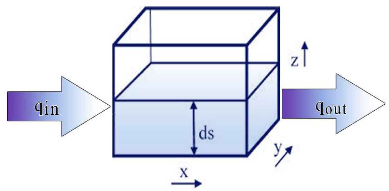
A water balance method was applied in a control volume under the condition of mass conservation to evaluate the overflow discharge from paddy fields. From a three-dimensional microcosmic view (Figure 1), the porosity medium flow condition can be given as in Equation (1):

$${\mathrm{q}}_{\mathrm{in}}-{\mathrm{q}}_{\mathrm{out}}=\frac{\mathrm{ds}}{\mathrm{dt}}$$

(1)

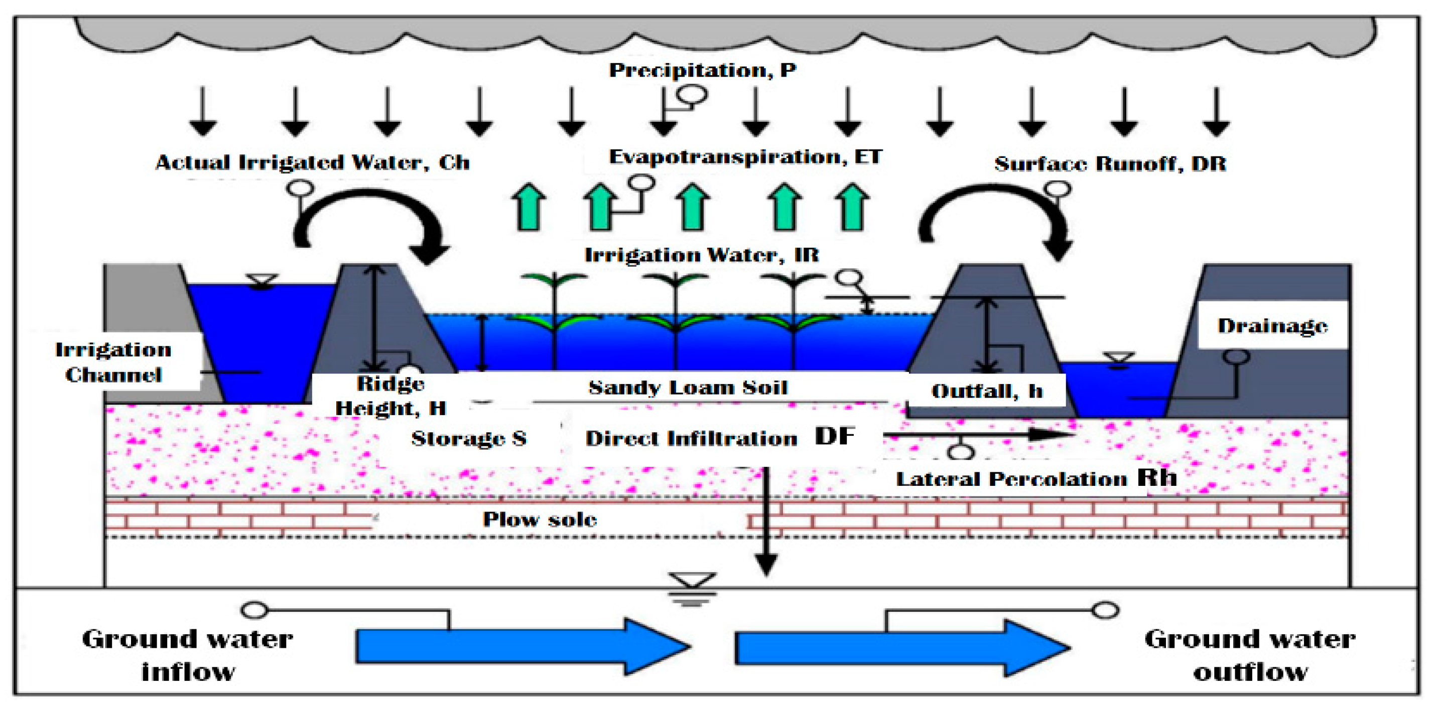
where ${\mathrm{q}}_{\mathrm{in}}$ is inflow, ${\mathrm{q}}_{\mathrm{out}}$ is outflow, $\mathrm{ds}$ is the change in storage of control volume with in a time t. The Conceptual model (Figure 2) of field water balance was formulated by considering the field as a linear reservoir; where, ${\mathrm{q}}_{\mathrm{in}}$ as a summation of the rainfall and irrigation; ${\mathrm{q}}_{\mathrm{out}}$ as a summation of crop evapotranspiration, surface runoff, shallow ground water outflow and infiltration; and $\mathrm{ds}$ as a summation of field ponding depth and shallow water content in the soil. The parameters, rainfall and irrigation, decrease the depletion in root zone by adding water, while the increase in depletion is received by removing water in root zones by the components such as crop evapotranspiration, surface runoff and percolation [32].

Assuming that the paddy field is under cultivation and the plow pan exists, the water balance method is given by Equation (2). The decision criteria whether to irrigate or not is represented by Equations (3) and (4).

$$\begin{gathered} {\mathrm{S}}_{\mathrm{i}}={\mathrm{S}}_{\mathrm{i}-1}+{\mathrm{P}}_{\mathrm{i}}+{\mathrm{Ch}}_{\mathrm{i}}-{\mathrm{ET}}_{\mathrm{i}}-{\mathrm{DR}}_{\mathrm{i}}-{\mathrm{DF}}_{\mathrm{i}}-{\mathrm{Rh}}_{\mathrm{i}}, \\ \mathrm{If}{\mathrm{S}}_{\mathrm{i}-1}+{\mathrm{P}}_{\mathrm{i}}<{\mathrm{N}}_{\mathrm{i}},\mathrm{then}{\mathrm{IR}}_{\mathrm{i}}>0 \\ \mathrm{If}{\mathrm{S}}_{\mathrm{i}-1}+{\mathrm{P}}_{\mathrm{i}}\ge {\mathrm{N}}_{\mathrm{i}},\mathrm{then}{\mathrm{IR}}_{\mathrm{i}}=0 \end{gathered}$$

(2)

$$\begin{gathered} {\mathrm{N}}_{\mathrm{i}}={\mathrm{ET}}_{\mathrm{i}}+{\mathrm{DF}}_{\mathrm{i}}+{\mathrm{Rh}}_{\mathrm{i}} \\ \mathrm{If}{\mathrm{Ri}}_{\mathrm{i}}\ge {\mathrm{IR}}_{\mathrm{i}},\mathrm{then}{\mathrm{Ch}}_{\mathrm{i}}={\mathrm{IR}}_{\mathrm{i}} \\ \mathrm{If}{\mathrm{Ri}}_{\mathrm{i}}<{\mathrm{IR}}_{\mathrm{i}},\mathrm{then}{\mathrm{Ch}}_{\mathrm{i}}={\mathrm{Ri}}_{\mathrm{i}} \end{gathered}$$

(3)

$${\mathrm{IR}}_{\mathrm{i}}={\mathrm{St}}_{\mathrm{i}}-({\mathrm{S}}_{\mathrm{i}-1}+{\mathrm{P}}_{\mathrm{i}})+{\mathrm{N}}_{\mathrm{i}}$$

(4)

where the suffixes i and i − 1 represent the time period. ${\mathrm{S}}_{\mathrm{i}}$ is field storage, ${\mathrm{S}}_{\mathrm{i}-1}$ is previous field storage, P is rainfall, Ch is channel irrigation water applied, ET is actual crop evapotranspiration, DR is surface runoff/overflow from field, DF is vertical percolation, and Rh lateral seepage inflow.

N represents the field losses from the system, IR is the irrigation water requirement $\mathrm{Ri}$ is channel water volume. The target depth of storage (St) equals the summation of ponding depth and soil saturation depth. All the components have same units (in terms of volume of water per unit area, or equivalent depth units).

The soil water content depends on the soil type. In the study area, soil type is sandy loam with average soil porosity of 43% and a coefficient of conductivity of 0.01158 (${\mathrm{d}}^{-1}$). The other characteristics include field capacity (14%) and wilting point (6 mm).

2.2. Crop Evapotranspiration

Crop water requirement and crop evapotranspiration are identical because during plant growth, the consumptive use of water is considered small and neglected while most of the water is lost via transpiration from the stomata. In a cropping field, transpiration from plants and evaporation from soil surface occurs at the same time and is not easy to measure separately. The combined term of evaporation and transpiration is called crop evapotranspiration, ${\mathrm{ET}}_{\mathrm{c}}$ $(\mathrm{mm}·{\mathrm{d}}^{-1})$. ${\mathrm{ET}}_{\mathrm{c}}$ can be determined by direct measurement or indirect calculations, while the direct measurement method is expensive due to morphological limitations. Therefore, indirect calculation method is used under standard conditions as given in Equation (5):

$${\mathrm{ET}}_{\mathrm{c}}={\mathrm{K}}_{\mathrm{c}}\times {\mathrm{ET}}_0$$

(5)

where ${\mathrm{K}}_{\mathrm{c}}$ is a single crop coefficient, ${\mathrm{ET}}_0$ is the reference crop evapotranspiration. In general, the crop coefficient is approximately 0.95–1.35 for paddy rice, while FAO (Food and Agriculture Organization), also recommended the ${\mathrm{K}}_{\mathrm{c}}$ value for the 1st and 2nd crop period [32]. In this study the ${\mathrm{K}}_{\mathrm{c}}$ values were used from Yao et al., listed in

Table 1. Paddy rice crop coefficient (K_c) for each growth stage adopted from Yao et al. [33].

Growth Days	Growth Stage	Growth Degree	Crop Season
			1st Crop	2nd Crop
—	Ground	—	—	—
1~15	Seedling	185	0.92	1.01
16~30	Early tillering	381	1.00	1.11
31~45	End of tillering	589	1.00	1.11
46~60	Early flowering	808	1.13	1.23
61~75	End of flowering	1032	1.13	1.23
76~90	Early ripening	1259	0.89	0.93
91~105	Middle of ripening	1487	0.89	0.93
106~120	End of ripening	1715	0.89	0.93

because of avoiding climate change due to regional differences, and also the availability of corresponding crop coefficient with different crop growth stages of paddy rice from experiments [33].

The Penman-Monteith equation is a suitable and recommended method for estimating the ${\mathrm{ET}}_0$ by Allen et al., and the details are available in FAO irrigation and drainage paper No. 56 [32]. According to Smith et al., ${\mathrm{ET}}_0$ estimation results are more consistent with the Penman-Monteith method and performance is better than other ${\mathrm{ET}}_0$ methods when compared with lysimeter data [34]. The Penman-Monteith equation is given in Equation (6)

$${\mathrm{ET}}_0=\frac{0.408\Delta \left({\mathrm{R}}_{\mathrm{n}}-\mathrm{G}\right)+\mathsf{\gamma }\frac{900}{\mathrm{T}+273}{\mathrm{U}}_2\left({\mathrm{e}}_{\mathrm{s}}-{\mathrm{e}}_{\mathrm{a}}\right)}{\Delta +\mathsf{\gamma }\left(1+0.34{\mathrm{U}}_2\right)}$$

(6)

where ${\mathrm{ET}}_0$ is the reference crop evapotranspiration (mm$·$d⁻¹); ${\mathrm{R}}_{\mathrm{n}}$ is the net radiation at the crop surface ($\mathrm{MJ}·{\mathrm{m}}^{-2}·{\mathrm{d}}^{-1}$); $\mathrm{G}$ is the heat flux of soil ($\mathrm{MJ}·{\mathrm{m}}^{-2}·{\mathrm{d}}^{-1}$); $\mathrm{T}$ is the mean daily temperature at 2-m height (°C); ${\mathrm{U}}_2$ is the measured wind velocity at 2 m height ($\mathrm{m}·{\mathrm{s}}^{-1})$; ${\mathrm{e}}_{\mathrm{s}}$ is the saturation vapor pressure ($\mathrm{kPa}$); ${\mathrm{e}}_{\mathrm{a}}$ is the actual vapor pressure ($\mathrm{kPa}$); ${\mathrm{e}}_{\mathrm{s}}-{\mathrm{e}}_{\mathrm{a}}$ is the vapor pressure deficit ($\mathrm{kPa}$); $\Delta$ is the gradient of saturated vapor pressure ($\mathrm{kPa}·{°\mathrm{C}}^{-1}$); $\mathsf{\gamma }$ is psychrometric the constant of humidity ($\mathrm{kPa}·{°\mathrm{C}}^{-1}$).

When the value of ${\mathrm{K}}_{\mathrm{c}}$ is determined according to the crop type and the growth stage, wilting point (${\mathrm{W}}_{\mathrm{p}}$) plays a key role in determining the occurrence of evapotranspiration. It implies that the plant cannot absorb any more water from its root. Thus, the crop evapotranspiration can be represented using the conditions of Equations (7) and (8).

$${\mathrm{ET}}_{\mathrm{i}}=\{\begin{array}{c}{\mathrm{K}}_{\mathrm{C}}\times {\mathrm{ET}}_0\mathrm{if}{\mathrm{S}}_{\mathrm{i}-1}>{\mathrm{W}}_{\mathrm{p}}\\ 0\mathrm{if}{\mathrm{S}}_{\mathrm{i}-1}<{\mathrm{W}}_{\mathrm{p}}\end{array}$$

(7)

$${\mathrm{W}}_{\mathrm{p}}=\mathrm{Soil}\mathrm{depth}\times \mathrm{Wilting}\mathrm{point}$$

(8)

where ${\mathrm{W}}_{\mathrm{p}}$ denotes the depth of wilting point (mm).

2.3. Irrigation Water Demand

The irrigation water requirement varies with the growth of the paddy crop, and the irrigation water is controlled with an adjustment mechanism of the field water gates. During the time of irrigation, the field conveyance and channel conveyance losses should be considered in the amount of irrigation water required. This can be regarded as the difference between the amount of ponding depth and the summation of previous field storage after deduction losses and precipitation of the day. Considering the conveyance loss during the time of irrigation, the actual irrigation water amount is the summation of irrigation water demand and the conveyance loss, which can be described as in Equations (9) and (10).

$$\mathrm{Water}\mathrm{Conveyance}\mathrm{loss}=\frac{\mathrm{Irrigation}\mathrm{water}\mathrm{demand}}{\left(1-\mathrm{Water}\mathrm{conveyance}\mathrm{loss}\mathrm{rate}\right)}-\mathrm{Irrigation}\mathrm{water}\mathrm{demand}$$

(9)

$$\mathrm{Actual}\mathrm{irrigation}\mathrm{water}=\mathrm{Irrigation}\mathrm{water}\mathrm{demand}+\mathrm{Water}\mathrm{conveyance}\mathrm{loss}$$

(10)

The conveyance loss is calculated by considering the length of each channel from the intake gate to each sub-block (the detail is given in Section 3.1), and the loss rate of 10% for every kilometer was considered as the conveyance loss, as shown in

Table 2. Water conveyance loss calculation from the intake gate to each sub-block (unit: %).

	Conveyance Loss (%)	Block 1	Block 2	Block 3	Block 4	Block 5
Sub-Block
No. 1		8.15	13.15	20.23	21.16	28.5
No. 2		8.15	13.15	20.23	24.93	28.5
No. 3		10.45	11.9	22.01	24.93	29.33
No. 4		10.45	11.9	22.01	33.33	29.33
No. 5		11.71	19.08	22.85	—	30.38
No. 6		11.71	19.08	—	—	30.38
No. 7		12.74	21	—	—	—
No. 8		12.74	21	—	—	—

.

2.4. Percolation Calculation

Percolation is the downward movement of water towards the horizontal hydraulic gradient and the vertical direction through porous media up to the groundwater table [27]. It is a complex process in a paddy field and is influenced by factors such as soil texture, ponding depth, depth to ground water level, water temperature, terrain slope, crop root zone depth, presence of plow pan or hard layer below surface, and subsoil hydraulic conductivity. It is the summation of vertical percolation and lateral seepage, which are described below.

2.4.1. Vertical Percolation

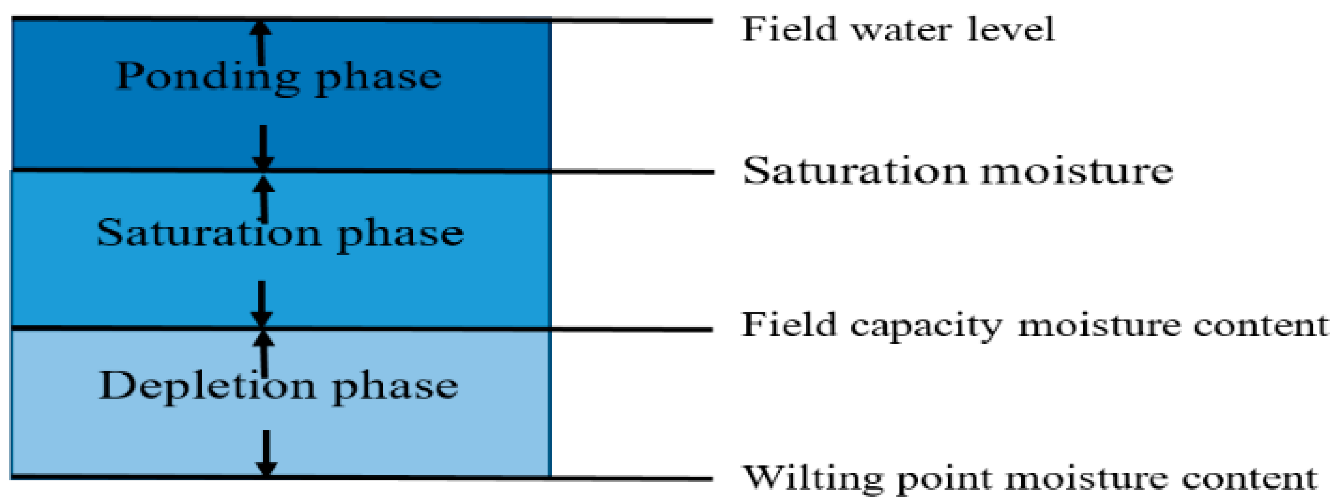
Experimental results under different irrigation conditions indicated that the plow pan leads to a decrease in the vertical and lateral percolation [35,36]. Vertical percolation is the deep percolation in which water, after passing through the plow pan, subsides to ground water table. The quantification of deep percolation from paddy field can be done under three different stages, as shown in Figure 3 [37]. The procedure for estimation of deep percolation for different phases is different such as in the ponding phase, the steady state flow equation is considered, while for saturation phase of crop, the calculations can be done using the method of Khepar et al. [38]. In the depletion phase the loss of deep percolation is assumed to be negligible [37]. Darcy Law is used for calculation of vertical percolation. The occurrence of vertical percolation depends on the comparison of field capacity (FC) and the previous field storage, as given in Equations (11)–(13). Let ${\mathrm{C}}_{\mathrm{p}}={\mathrm{k}}_{\mathrm{p}}/{\mathrm{l}}_{\mathrm{p}}$; then, P_t can be obtained as in Equation (14):

$${\mathrm{DF}}_{\mathrm{i}}=\{\begin{array}{c}{\mathrm{P}}_{\mathrm{t}}\mathrm{if}{\mathrm{S}}_{\mathrm{i}-1}>\mathrm{FC}\\ 0\mathrm{if}{\mathrm{S}}_{\mathrm{i}-1}\le \mathrm{FC}\end{array}$$

(11)

$$\mathrm{FC}=\mathrm{Soil}\mathrm{depth}\times \mathrm{Field}\mathrm{Capacity}$$

(12)

$${\mathrm{P}}_{\mathrm{t}}={\mathrm{k}}_{\mathrm{p}}\times \frac{{\mathrm{h}}_{\mathrm{t}}+{\mathrm{l}}_{\mathrm{m}}}{{\mathrm{l}}_{\mathrm{p}}}$$

(13)

$${\mathrm{P}}_{\mathrm{t}}={\mathrm{C}}_{\mathrm{p}}\times \left({\mathrm{h}}_{\mathrm{t}}+{\mathrm{l}}_{\mathrm{m}}\right)$$

(14)

where ${\mathrm{P}}_{\mathrm{t}}$ is the percolation $(\mathrm{mm}·{\mathrm{d}}^{-1})$; FC is the depth of Field Capacity (mm); ${\mathrm{K}}_{\mathrm{p}}$ is the coefficient of hydraulic conductivity $(\mathrm{mm}·{\mathrm{d}}^{-1})$; ${\mathrm{h}}_{\mathrm{t}}$ is the previous ponding depth (mm); ${\mathrm{l}}_{\mathrm{p}}$ denotes the thickness of plow pan (mm), which set as 7.5 cm [37]; ${\mathrm{l}}_{\mathrm{m}}$ denotes the thickness of muddy layer (mm); and ${\mathrm{C}}_{\mathrm{p}}$ denotes the coefficient of conductivity (${\mathrm{d}}^{-1}$) (Table 1).

2.4.2. Lateral Seepage

Lateral seepage flow occurs in a two ways through the paddy field bund/ridge, namely, (i) horizontal flow type, and (ii) downward flow type, and it is 10 times the vertical percolation. The lateral seepage should be considered with saturated and unsaturated field soil [35]. It is the horizontal loss sideways into the bunds or field boundaries which changes with the length of the bund, the area of the paddy field, and the initial soil water content. Lateral seepage/percolation is considered as additional field loss because under the bund of field there is no continuous plow pan layer, consequently, the water movement is easy into and down through the bund to underlying water table. Several past studies showed the way of measuring lateral seepage using ponding tests and other water balance experiments such as [35,39,40,41,42,43].

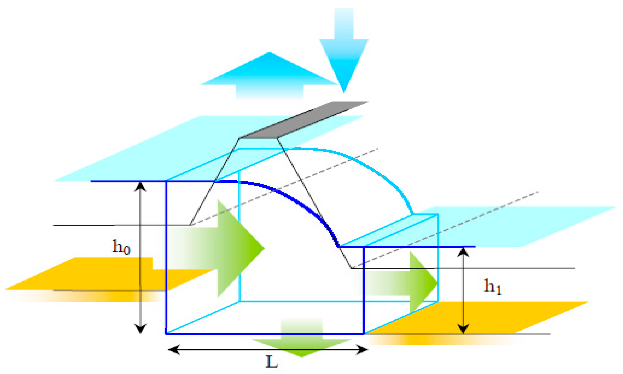
This study assumes that the lateral seepage occurs under saturated conditions, and the terminal of seepage should be the groundwater level. The schematic of ridge lateral seepage is shown in Figure 4. The transmission mechanism derived from the Dupuit equation, as shown in Equation (15):

$${\mathrm{L}}_{\mathrm{t}}=\frac{{\mathrm{l}}_{\mathrm{g}}}{\mathrm{A}}\times {\mathrm{k}}_{\mathrm{L}}\times \frac{\left({\mathrm{h}}_{\mathrm{t}}^2-{\mathrm{h}}_0^2\right)}{2\mathrm{L}}$$

(15)

where ${\mathrm{l}}_{\mathrm{g}}$ is the length of the ridge near a drainage (m) and is set as the side length of each paddy block in this study; $\mathrm{A}$ denotes the area of the paddy field (${\mathrm{m}}^2$); ${\mathrm{K}}_{\mathrm{L}}$ denotes the hydraulic conductivity of the ridge $\left(\mathrm{mm}·{\mathrm{d}}^{-1}\right)$, set as five times ${\mathrm{K}}_{\mathrm{p}}$; ${\mathrm{h}}_{\mathrm{t}}$ is the ponding depth (mm); ${\mathrm{h}}_0$ denotes the water level of the irrigation channel (mm), set as 0 cm; and $\mathrm{L}$ denotes the width of the ridge (mm), set as 50 cm. Field capacity (FC) plays an important role in the calculation of lateral seepage, as the condition criteria is in Equation (16).

$${\mathrm{Rh}}_{\mathrm{i}}=\{\begin{array}{c}{\mathrm{L}}_{\mathrm{t}}\mathrm{if}{\mathrm{S}}_{\mathrm{i}-1}>\mathrm{FC}\\ 0\mathrm{if}{\mathrm{S}}_{\mathrm{i}-1}\le \mathrm{FC}\end{array}$$

(16)

where $\mathrm{Rh}$ denotes the lateral seepage of the ridge $\left(\mathrm{mm}·{\mathrm{d}}^{-1}\right)$ and ${\mathrm{L}}_{\mathrm{t}}$ denotes the lateral infiltration ($\mathrm{mm}·{\mathrm{d}}^{-1}$).

2.5. Field Surface Runoff Calculation

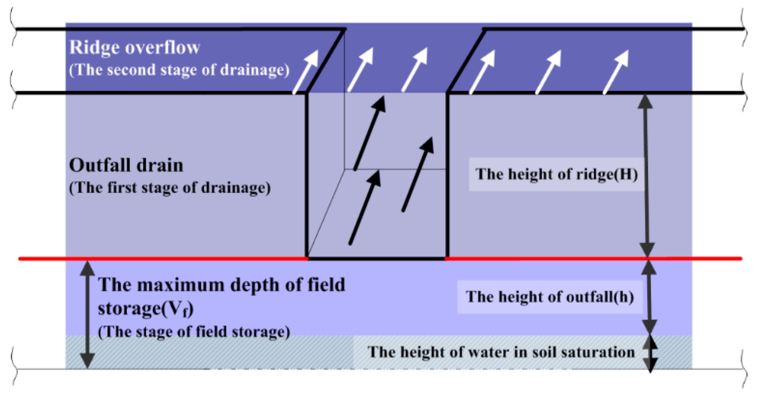
The ponding depth required for paddy rice must be adjusted suitably during different growth stages, and it is controlled by the height of outfall on the ridge. The height of the ridge and outfall are the average elevation difference between the elevation of the ridge and outfall, respectively, and the height of the outfall determines the magnitude of field storage. After saturation condition, the inflow (irrigation and rain water) behaves as a field surface runoff and it overflows the ridge to the drainage when the ponding depth is higher than the outfall or ridge, as shown in Figure 5. The surface runoff is a function of rainfall having a positive correlation [44], while it is reduced by carefully maintaining the ridge up to certain height for proper ponding. The hydrological simulation model developed by Ray-Shyan Wu et al., for rice paddy fields indicated that surface runoff may occur when the depth of rainwater exceeds the height of ridge, and it was analyzed that the amount of surface runoff from paddy field is about 27% of the amount of rainfall [45].

The height of the outfall depends on the paddy rice cultivation in different stages of the first crop season in Taiwan, as given in

Table 3. Ponding depth during the first crop season of paddy rice in Taiwan.

Growth Stages	Seedling			Start of Tillering	End of Tillering	Young Panicle Differentiation	Young Panicle Formation	Booting Stage	Heading	Milk Ripe	Mature	Reaping
The day after transplanting	1	16	25	30	48	50	65	77	92	107	120	130
Date	3/4	3/19	3/28	4/2	4/20	4/22	5/7	5/19	6/3	6/18	7/1	7/11
Ponding depth (cm)	5	5	5	5	5	5	10	10	10	3	3	0

[35]. The outflow of the field runoff can be represented as in Equations (17)–(19).

$$\begin{gathered} {\mathrm{DR}}_{\mathrm{i}}={\mathrm{S}}_{\mathrm{i}-1}+{\mathrm{P}}_{\mathrm{i}}+{\mathrm{Ch}}_{\mathrm{i}}-{\mathrm{ET}}_{\mathrm{i}}-{\mathrm{DF}}_{\mathrm{i}}-{\mathrm{Rh}}_{\mathrm{i}}-{\mathrm{V}}_{\mathrm{fi}} \\ \mathrm{if}{\mathrm{S}}_{\mathrm{i}-1}+{\mathrm{P}}_{\mathrm{i}}+{\mathrm{Ch}}_{\mathrm{i}}-{\mathrm{ET}}_{\mathrm{i}}-{\mathrm{DF}}_{\mathrm{i}}-{\mathrm{Rh}}_{\mathrm{i}}>{\mathrm{V}}_{\mathrm{fi}} \end{gathered}$$

(17)

$${\mathrm{DR}}_{\mathrm{i}}=0,\mathrm{if}{\mathrm{S}}_{\mathrm{i}-1}+{\mathrm{P}}_{\mathrm{i}}+{\mathrm{Ch}}_{\mathrm{i}}-{\mathrm{ET}}_{\mathrm{i}}-{\mathrm{DF}}_{\mathrm{i}}-{\mathrm{Rh}}_{\mathrm{i}}\le {\mathrm{V}}_{\mathrm{fi}}$$

(18)

$${\mathrm{V}}_{\mathrm{f}}=\left(\mathrm{h}+\mathrm{Soil}\mathrm{depth}\times \mathsf{\phi }\right)$$

(19)

where ${\mathrm{V}}_{\mathrm{f}}$ is the depth of field storage (mm), which is the total height of water in soil saturation and outfall; $\mathrm{DR}$ is the outflow of the field runoff (mm); $\mathrm{h}$ is the height of outfall (mm); and $\mathsf{\phi }$ is soil porosity (%).

For the extended duration of rain, the depth of storage may be higher than the height of the outfall, and the maximum outflow of the ridge should be computed to avoid any effect on the growth of the crop roots. The factors related with the outflow include the rainfall, area, crop soaking time, and the period of drainage. The average overflow discharge can be calculated using Equations (20)–(23).

$${\mathrm{Q}}_{\mathrm{i}}=\frac{\mathrm{C}\times {\mathrm{R}}_{\mathrm{D}}}{1000\times \mathrm{D}}{\mathrm{if}\mathrm{P}}_{\mathrm{i}}>{\mathrm{Q}}_{\mathrm{i}}+{\mathrm{ET}}_{\mathrm{i}}+{\mathrm{DF}}_{\mathrm{i}}+{\mathrm{Rh}}_{\mathrm{i}}$$

(20)

$$\begin{gathered} {\mathrm{DR}}_{\mathrm{i}}={\mathrm{S}}_{\mathrm{i}-1}+{\mathrm{P}}_{\mathrm{i}}+{\mathrm{Ch}}_{\mathrm{i}}-{\mathrm{ET}}_{\mathrm{i}}-{\mathrm{DF}}_{\mathrm{i}}-{\mathrm{Rh}}_{\mathrm{i}}-{\mathrm{V}}_{\mathrm{fi}}^{\prime } \\ \mathrm{if}{\mathrm{S}}_{\mathrm{i}-1}+{\mathrm{P}}_{\mathrm{i}}+{\mathrm{Ch}}_{\mathrm{i}}-{\mathrm{ET}}_{\mathrm{i}}-{\mathrm{DF}}_{\mathrm{i}}-{\mathrm{Rh}}_{\mathrm{i}}>{\mathrm{V}}_{\mathrm{fi}}^{\prime } \end{gathered}$$

(21)

$$\begin{gathered} {\mathrm{DR}}_{\mathrm{i}}=\min \left[{\mathrm{Q}}_{\mathrm{i}}；{\mathrm{S}}_{\mathrm{i}-1}+{\mathrm{P}}_{\mathrm{i}}+{\mathrm{Ch}}_{\mathrm{i}}-{\mathrm{ET}}_{\mathrm{i}}-{\mathrm{DF}}_{\mathrm{i}}-{\mathrm{Rh}}_{\mathrm{i}}-{\mathrm{V}}_{\mathrm{fi}}\right] \\ \mathrm{if}{\mathrm{S}}_{\mathrm{i}-1}+{\mathrm{P}}_{\mathrm{i}}+{\mathrm{Ch}}_{\mathrm{i}}-{\mathrm{ET}}_{\mathrm{i}}-{\mathrm{DF}}_{\mathrm{i}}-{\mathrm{Rh}}_{\mathrm{i}}\le {\mathrm{V}}_{\mathrm{fi}}^{\prime } \end{gathered}$$

(22)

$${\mathrm{V}}_{\mathrm{f}}^{\prime }=\left(\mathrm{H}+\mathrm{Soil}\mathrm{depth}\times \mathsf{\phi }\right)$$

(23)

where ${\mathrm{V}}_{\mathrm{f}}\prime$ is the maximum depth of field storage (mm), which is the total height of water in soil saturation and ridge; $\mathrm{Q}$ is the outflow in unit area (mm); D is the crop soaking time (d), set as three days in this study; C is the runoff coefficient (C = 0.6); R_D is continuous rainfall in D days (mm), according to the Xi-Zhou rainfall station with a 10-year return period, which is 294.5 $\mathrm{mm}·{\mathrm{d}}^{-1}$; and H is the height of the ridge (mm).

3. System Dynamic Model: VENSIM

The calculation of irrigation and drainage discharge are the prerequisite for the verification of the water balance approach of any irrigation canal command area, and it must have separate canal and drainage systems. The experimental study area has the same aforementioned elements, like irrigation channels to irrigate and to drain channels to drain overflow from each paddy field. In addition, a main drainage passes through the middle and accommodates surplus water from every drain, which is helpful for calculating the total drainage discharge. When the amount of rainfall or irrigation water is less than the crop water requirement, there is no overflow due to height of the ridge. However, during heavy rainfall paddy fields, drains the extra water through the outfall on the ridge to drain channels. A system dynamic VENSIM model was established and used to simulate the water demand and consumption of an experimental site in Central Taiwan. The description of study area and model setup are explained herein.

3.1. Study Area Overview

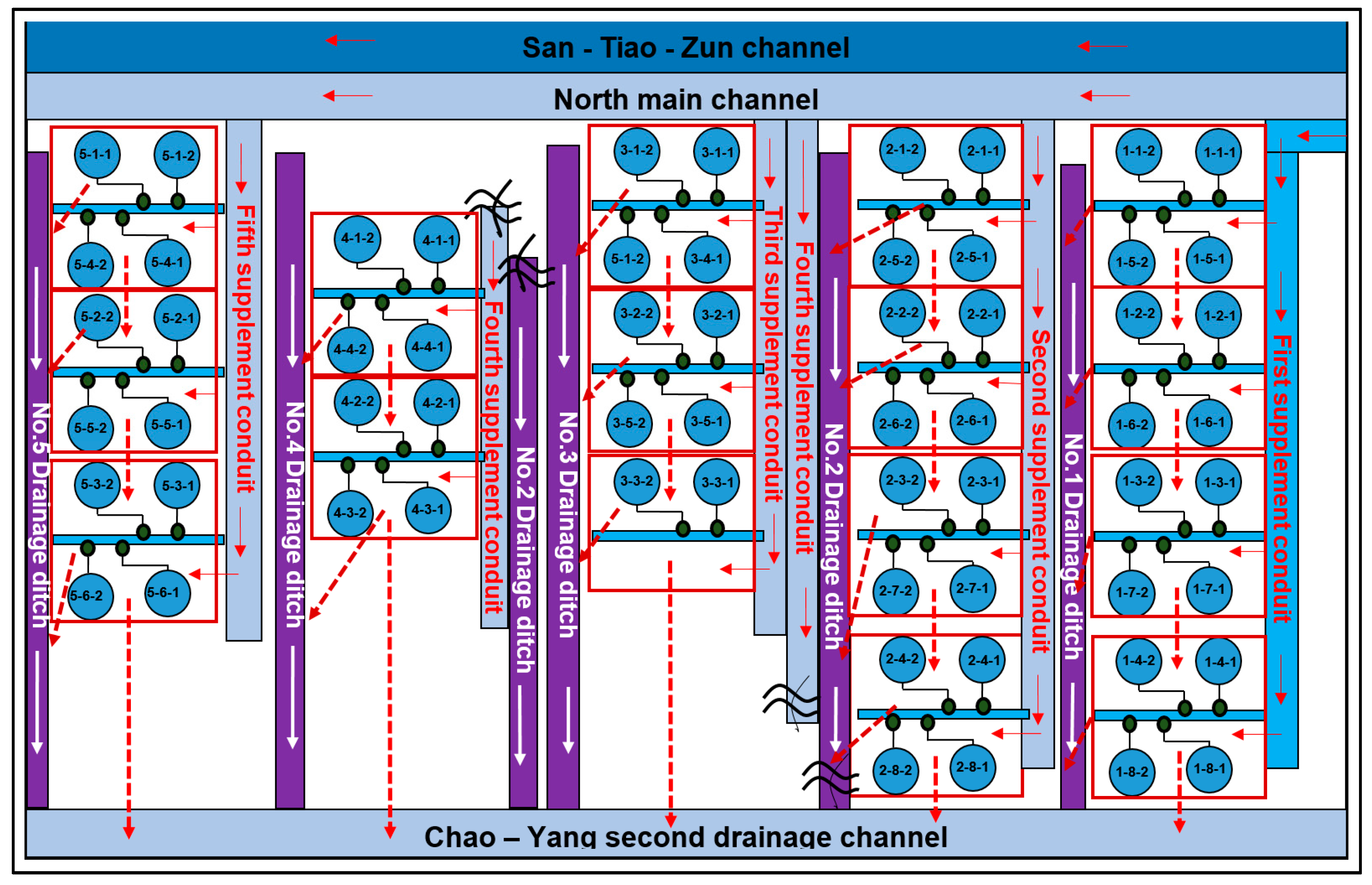
The study area is located in Chang-Hua County in Central Taiwan and has the Zhou-Shui-Xi River as its main water resource. For achieving precision irrigation, the study considers the irrigated area of the Shin-Yong-Chi channel, which receives water from the second restricted gate of the Tzu-Tsai-Pi channel. For controlling the quantity of irrigation, we selected a small area of 215 ha under the San-Tiao-Zun channel irrigation region, which belongs to the Shin-Yong-Chi main channel irrigation system. There are five supplement ditches in the area, corresponding to blocks 1 through 5, respectively. The soil type of the study region is sandy loam. There are six field monitoring stations for water level monitoring that correspond to blocks 1 through 5. The block 2 equipped has two stations for data monitoring. The stations in the field were powered by solar panel, the sensors detect water level and the recorder transfers water level information to data center every 10 min. After obtaining field water level information, the field water demand model calculates the target flow for the San-Tiao-Zun inflow station and operates the gate to meet the target flow. The layout of the experimental site is shown in Figure 6.

3.2. Model Establishment

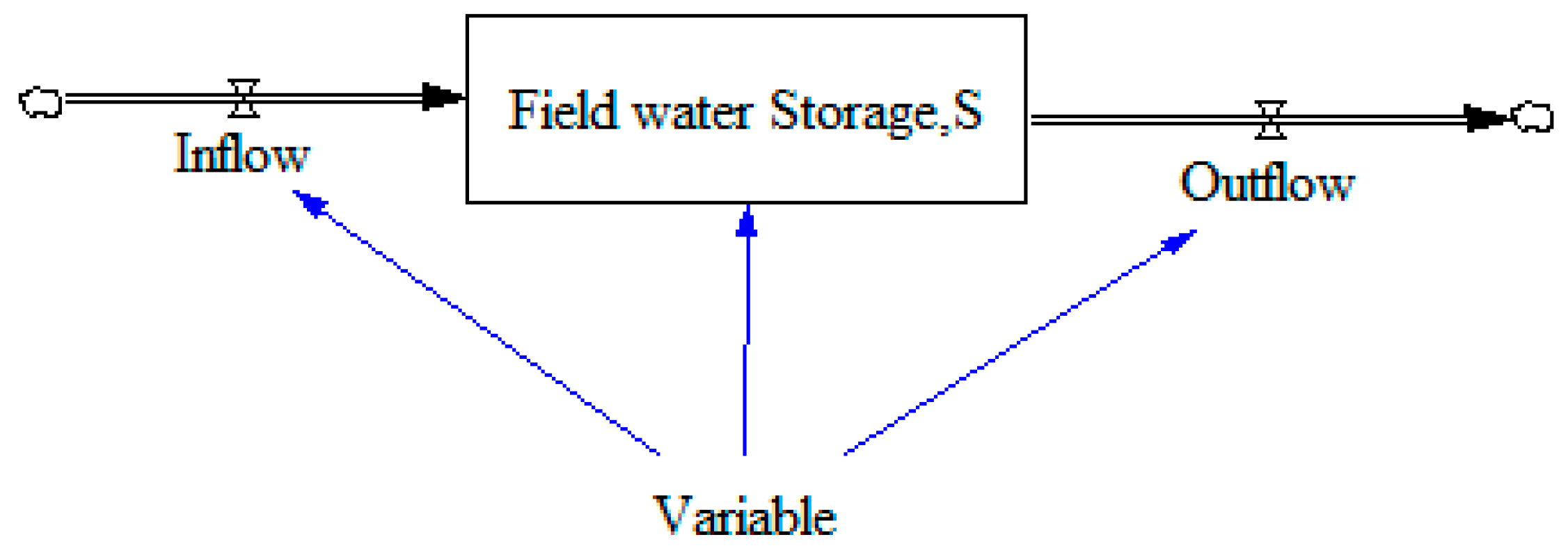
The system dynamic program, VENSIM, combines the theories of cybernetics, system theory, information theory, decision theory, and computer simulation. There are four main components to be used in description of the dynamic change in the system; the relation between each component is linked by an arrow line. These components are explained as follows.

• Level: Also called accumulated amount, the accumulation of flow inside the system, which indicates the variable’s situation in a moment, for example, field storage; integral calculus in mathematics.
• Rate: Also called rate amount, which implies the in or out storage flow. The value is obtained by function calculation; differential calculus in mathematics.
• Auxiliary: Its main function is to describe the relation between Level and Rate, and makes the system structure more clear. Another function is that of test value or test function.
• Arrow: It is used to connect auxiliary and flow formula.

The relation between each component is shown in Figure 7, and the variable-type mapping to components is listed in

Table 4. Component definition of the system dynamic model.

Symbol	Variable Definition	Component Description	Remark
	Storage in the system	Storage	Initial value
		Components
	Flow rate or storage rate	Flow Rate	Figures, tables, functions or logics are acceptable
		Components
	The assistant variables between storage and flow	Auxiliary
	The connection of information and function in the system	Assistant	Connection
		Components
	The system boundary	—	—

. After inputting every component and parameter, the system dynamic model can run under different scenarios.

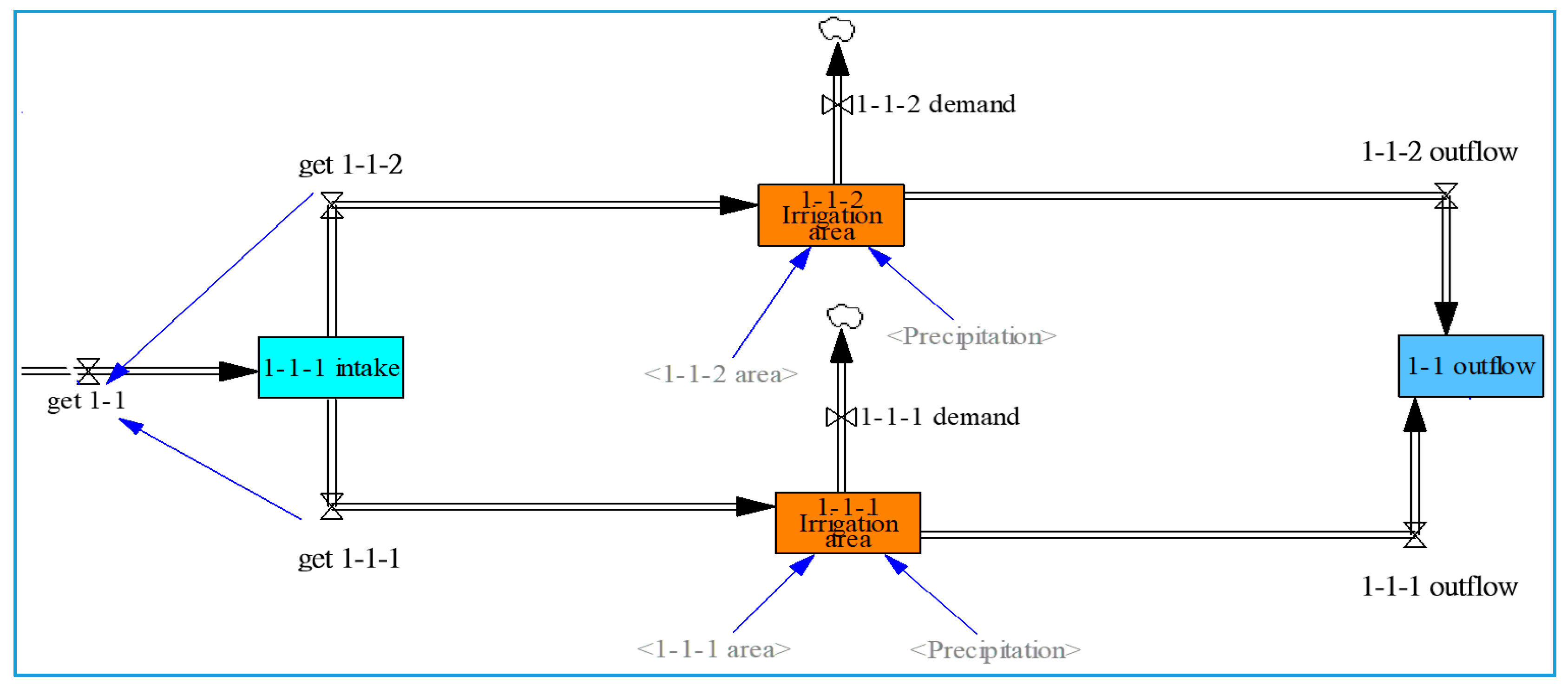
The study area comprised five irrigation blocks and 31 sub-blocks. The main motor-driven diversion gate, the San-Tiao-Zun inflow station and five manual gates downstream collect water into supplement ditches with the sequence from irrigation blocks 1 to 5 (Figure 8). The model was built based on the water balance principle to evaluate the irrigation water and field drainage. If the ponding depth reached the target value, the water supply would be stopped. The water usage sequence of the model is shown in Figure 9, where the boxes “1-1-1 irrigation area” and “1-1-2 irrigation area” mean the area of block 1-1 in paddy rice and upland crops, respectively. The study area consists of, mixed cropping system of 70% paddy rice and 30% upland crops.

The water flows with the block sequence, shown in Figure 10. If the depth of rainfall is less than the height of the outfall, there is no overflow to drain. However, if the rate of the rainfall is greater than the drain from the outfall, the water level may exceed the effective height of the ridge and overflow occurs. The water drains to the nearby field drain and converges to the main drain, Chao-Yang second drainage channel.

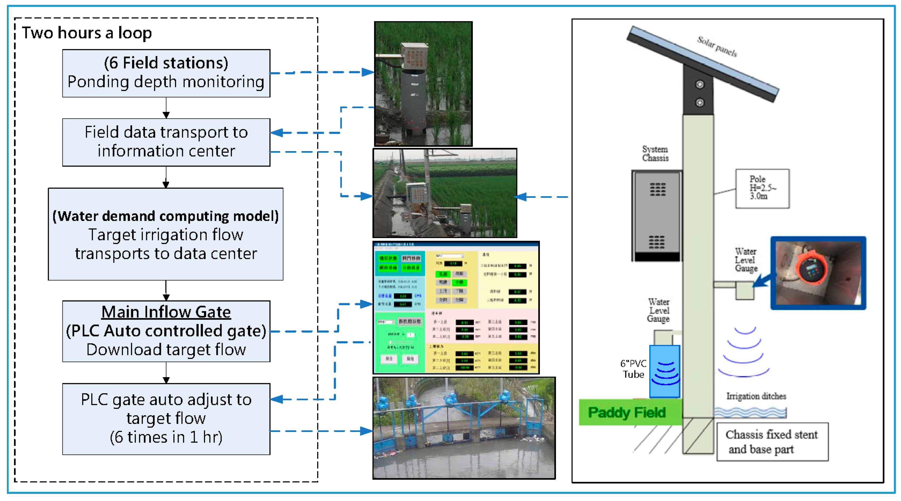
The procedure of field water demand model is represented in Figure 11. In addition to the basic soil texture established in the model, rainfall, irrigation water, and field ponding depth were obtained from the monitoring system. There are field monitoring stations set on the end of each block as shown in Figure 12. The sensors in the monitoring stations detect water level then record and transfer the information to the data center every 10 min. The field water demand model obtains field data from the data center, and computes the field overflow, infiltration, and evapotranspiration to estimate the flow of irrigation demand, which is transported to the data center within a cycle of two hours. The field ponding depth is simultaneously compared with the target depth. If the depth does not reach the target value in any one of the five blocks, the model calculates the difference in terms of water volume of that block and transmits the signal to the data center. The main inflow gate station, located at the upstream of the study area, equipped with an advanced programmable logic controller which downloads the required target flow from the data center every 10 min through the network, and the water gate is auto fine-tuned to attain the target flow.

3.3. Model Verification

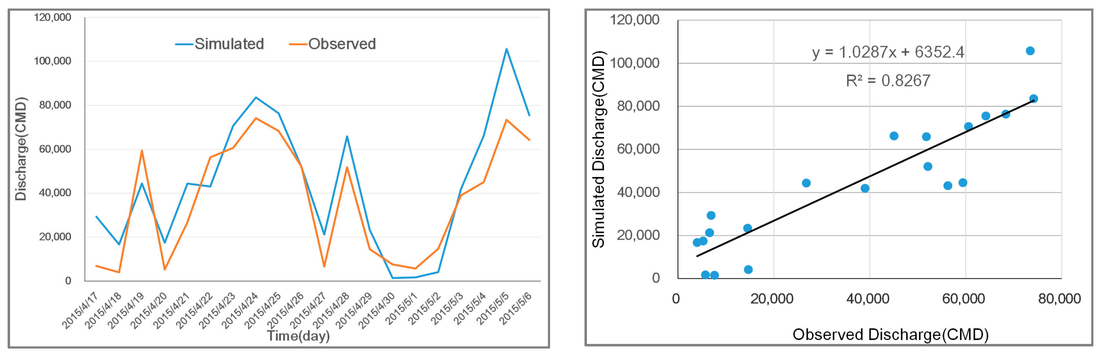
To verify the model, the coefficient of correlation (R²) was used as a criterion. Based on the field station setting limitations, the discharge data was available during the experimental period ranges from 17 April 2015 to 6 May 2015. The discharge of the observed and simulated shows good fit in similarity with the coefficient of correlation R² equals 0.83 (Figure 13).

4. Results and Discussion

In times of a drought event, if the water allocated to agriculture must be reduced, the irrigation manager would reduce the irrigation water for each block depending on the growth stage and the drought tolerance of paddy rice. In principle, the management method includes stopping the supply of water in case of rainfall, or reducing irrigation to get through the drought event. Under this premise, the study investigated the water accessing relationship for each block under different reduction in irrigation. Two scenarios, 30% reduction and 50% reduction, were adopted to demonstrate the application of the model suggested and identify the consequences in such operation.

4.1. Scenario 1: 30% Reduction of Planned Irrigation Water

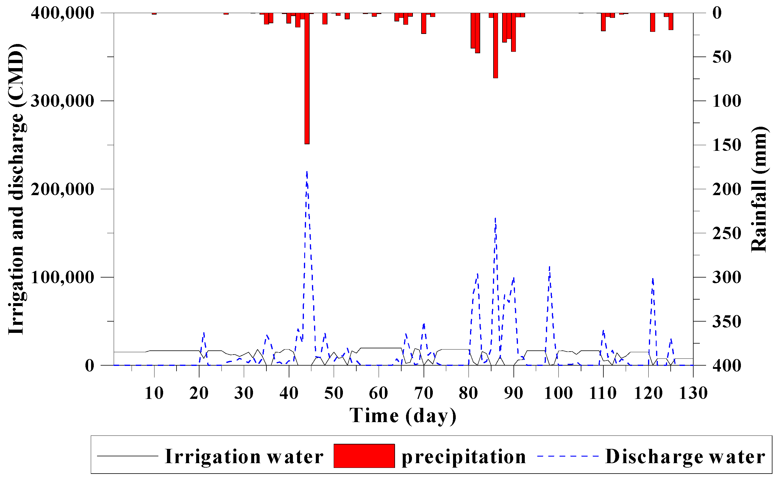
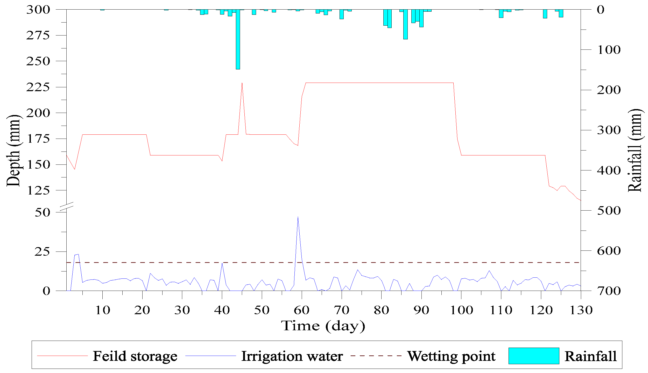
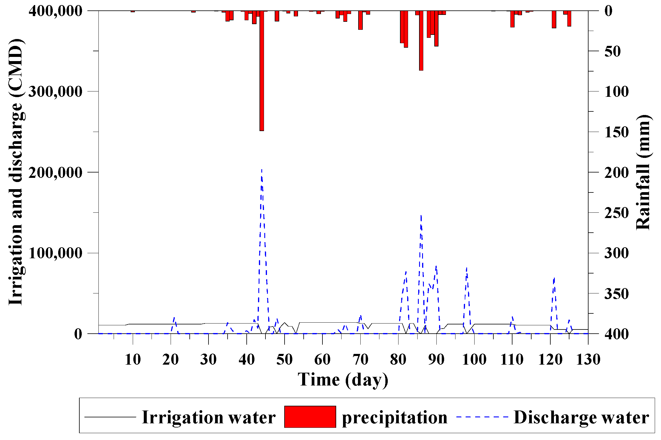
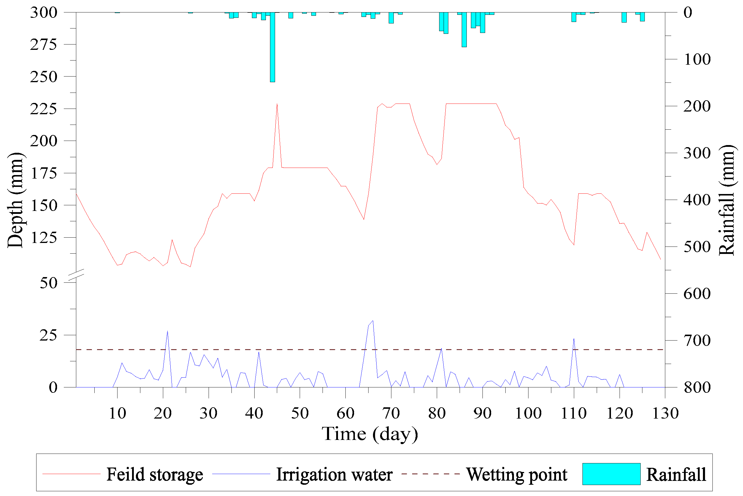
Scenario 1 assumes 30% of water reduction from the original irrigation plan during the first crop season. The simulation results are shown in Figure 14. It was depicted that, on 44th day the model stops irrigation due to 150 mm rainfall that produced maximum drainage discharge. From the 55th to the 63rd day, the irrigation meets the basic crop water requirement without producing any drainage discharge. There was continuous rainfall higher than 50 mm during the 80th to 100th day, which produce surface runoff, and the excess water was drained out. Until the 107th day, the target ponding depth changes to only 3 cm, and the model discharge surplus water even with a rainfall of 25 mm.

The simulation results of blocks 1–4 indicated that the target ponding depth with sufficient inflow of irrigation water was achieved within five days. The relative water distribution of blocks 1–4 is shown in Figure 15, Figure 16, Figure 17 and Figure 18. However, block 5 suffers up to the 9th day to meet the allocated water and is still not able to reach the target depth. The period from the 39th to 56th day is the rice booting, heading and milk ripe stage, which required more ponding depth, as shown in Figure 19. However, block 5 did not obtain sufficient water in this duration, which may lead to decline in rice productivity.

Although block 5 did not have sufficient irrigation water to satisfy the target ponding depth of every growth stage and the field storage curve remains away from its field capacity indicating that during the drought event, the 30% reduction does not affect the growth of paddy rice. Thus, it should be applied as a basic adjustment strategy. The simulated irrigation, discharge water, infiltration, and crop evapotranspiration of each block are listed in

Table 5. Simulation result of 30% reduction of planned irrigation water depth (mm) during the first crop season.

Block	30% Discount of Planned Irrigation Water	Total Irrigated Water	Rainfall	Infiltration	Discharge	Crop Evapotranspiration	$\frac{\mathbf{Discharge}}{\mathbf{Rainfall}}$	$\frac{\mathbf{Discharge}}{\left(\mathbf{Irrigated}\mathbf{water}\right)}$
1	1003.2	762.1	675	537.2	858.8	336.3	1.272	1.127
2		756.6	675	535.9		336.3		1.135
3		732.7	675	533.5		336.3		1.172
4		704.5	675	528.4		336.3		1.219
5		624.7	675	513.4		336.3		1.374

. Under 30% reduction of planned irrigation water, every block in the region has a discharge of 1.127–1.374 times the total irrigation water, indicating that much stricter polices may be considered.

4.2. Scenario 2: 50% Discount of Planned Irrigation Water

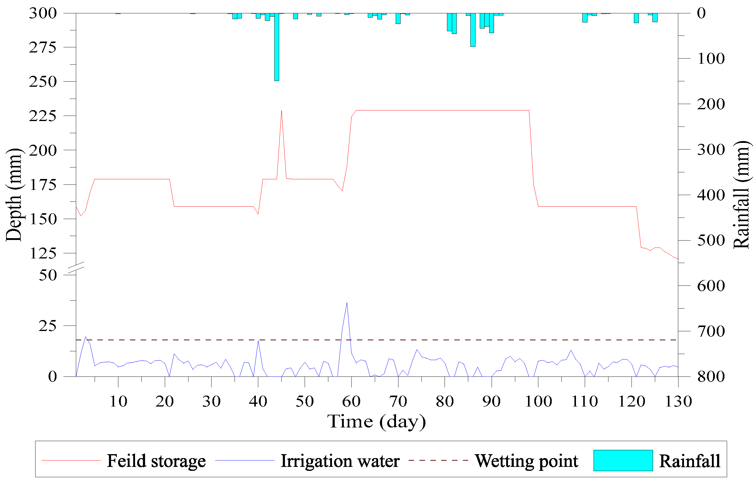
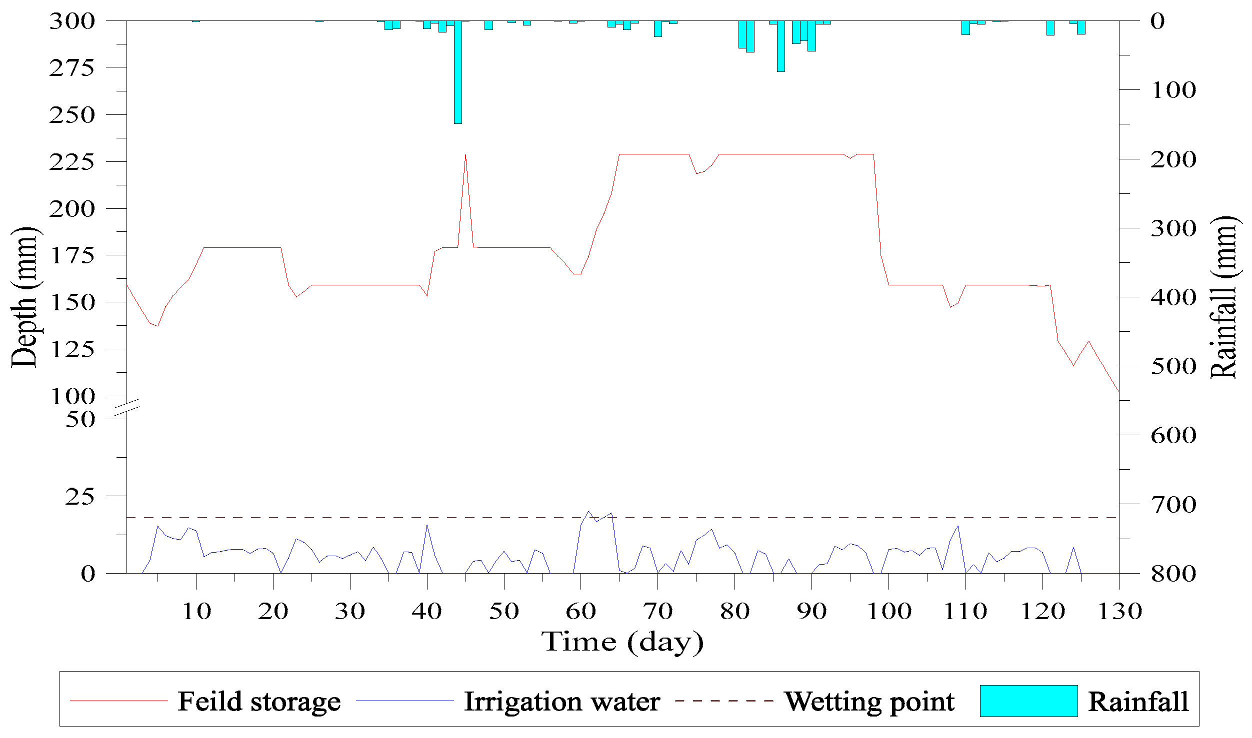
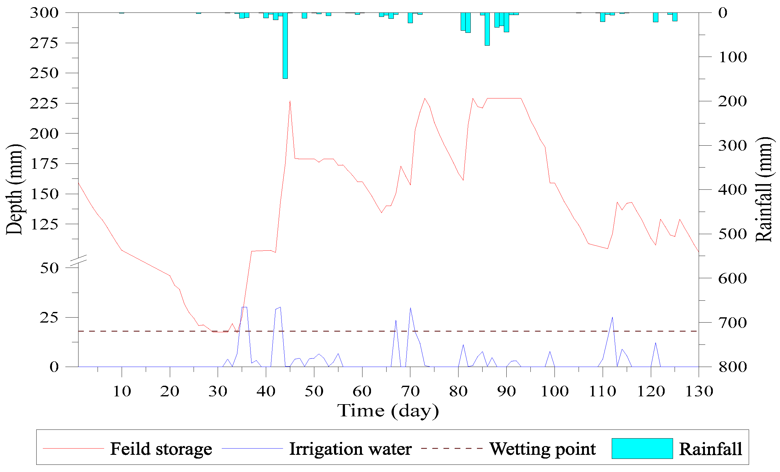
The second scenario simulates a drought period where it received 50% of the planned irrigation water. The drainage discharge decrease from the field due to less volume of water until rainfall occurrence on the 44th day, as shown in Figure 20. The simulation results according to block are described herein:

• The target ponding depth is 5 cm for the 1st day to 20th day cropping period. Blocks 1–3 reach this depth within 11 days, while block 4 reaches the target depth on the 34th day. The irrigation started in a sequence from upstream to downstream and reduces the issue of lack of water. The upstream fields receive the targeted depth irrigation and then transfer the water to downstream fields. The simulation results of targeted water depth of blocks 1–4 are shown in Figure 21, Figure 22, Figure 23 and Figure 24.
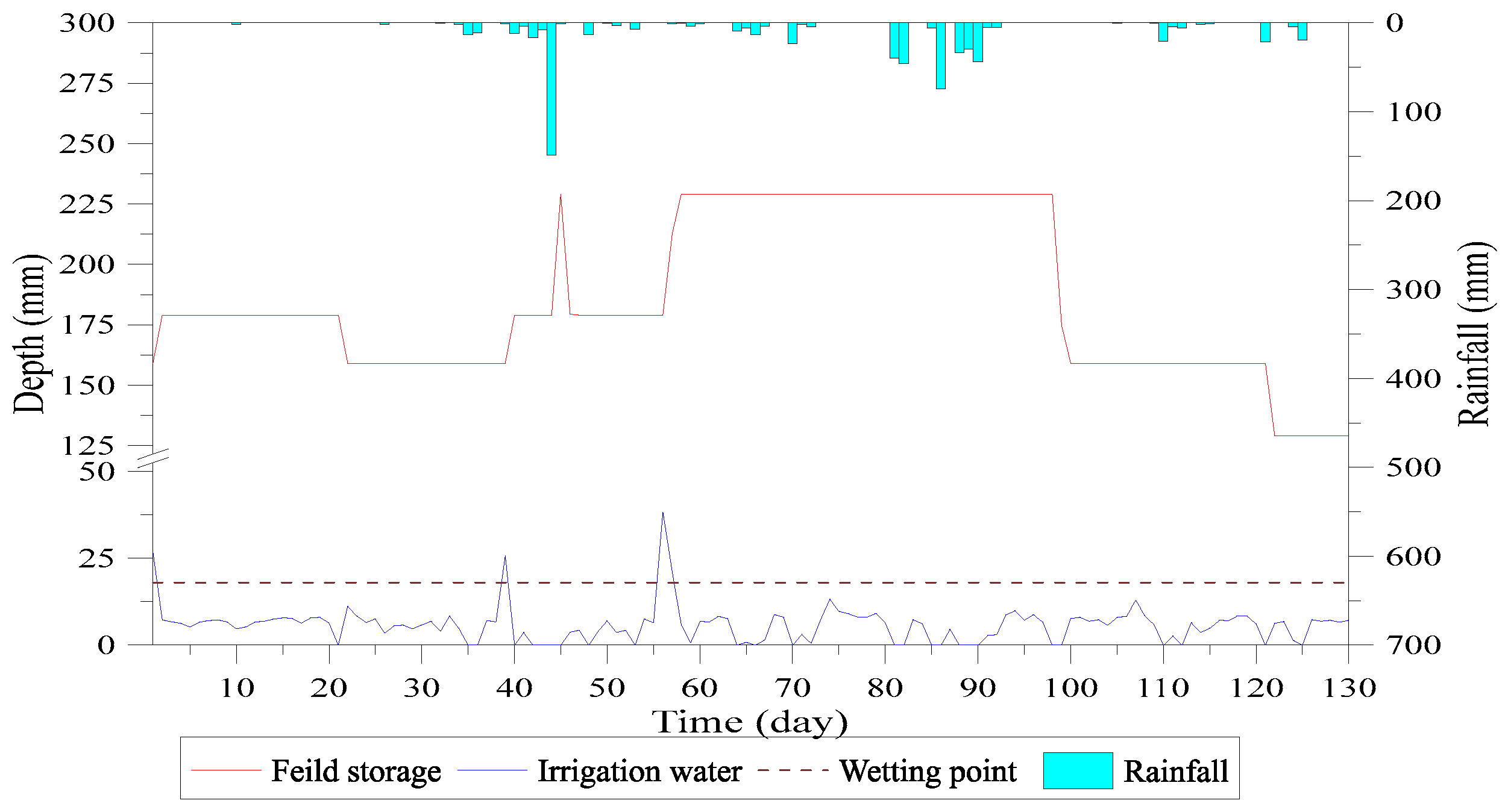
• The water depth of block 5 dropped below the saturated soil moisture curve on the 6th day due to lack of water. On the 21st day, the field storage turns lower than field capacity and the vertical percolation stopped. Up to the 29th day, the decrease in field storage continued and reached to the wilting point, also stopping the evapotranspiration, as shown in Figure 25.

The simulation results of scenario 2 indicated that only the block 5 could not obtain water and reached to wilting point. The possible strategy to pass through drought period and to supply required irrigation to all blocks, irrigate each block in rotation by adjusting all the gates and keep closing the gates of upstream blocks when there is no need of irrigation. In this way the downstream blocks may be ensured to receive the allocated irrigation water.

For the reduction of 50% water of the irrigation plan, the discharge of blocks 1–5 becomes 0.678–1.408 times the total irrigation water, as given in

Table 6. Simulation of 50% reduction of planned irrigation water depth (mm) during the first crop season.

Block	50% Discount of Planned Irrigation Water	Total Irrigated Water	Rainfall	Infiltration	Discharge	Crop Evapotranspiration	$\frac{\mathbf{Discharge}}{\mathbf{Rainfall}}$	$\frac{\mathbf{Discharge}}{\mathbf{Irrigated}\mathbf{water}}$
1	716.6	761.5	675	537.3	516.0	336.3	0.764	0.678
2		740.7	675	534.7		336.3		0.697
3		703.7	675	528.3		336.3		0.733
4		558.0	675	498.4		336.3		0.925
5		366.6	675	420.4		325.5		1.408

However, the 5th block discharges extra water due to the rainfall and before rainfall, and the rice plant may not survive.

5. Conclusions

This study applied the water balance method to establish water demand and a consumption model of an experimental site, and carried out the analysis of minimum irrigation water requirement. It achieves the coupling of field water monitoring system, the water demand estimation program and IoT (Internet of Things) technology. Wireless communication and systematized field water requirement models enabled this smart irrigation management to operate the field system through automatically identifying the field irrigation water depth and delivering the target flow by controlling field water gates through IoT.

The main crop in the study region was paddy rice, although approximately 30% of the area was cultivated with upland crops. Due to the fact that farmers are free to alter crops season to season, this irrigation management model is flexible enough to account for such changes. Scenario 1 analysis with 30% reduction of irrigation water indicated that the soil water content was less affected, which suggested such reduction can be the first step of policy implementation at the initiation of the drought event. Scenario 2 analysis with a 50% reduction in irrigation water can be applied as a solution of water shortage when the drought situation turns stricter. The results show that soil water content reached wilting point only occurred in the last block 5, which should be irrigated to avoid reaching the permanent wilting point before the 21st day. To achieve this, every block should be irrigated in rotation, by adjusting all gates more frequently to ensure that the downstream blocks can receive the allocated irrigation water.

In the future, innovative model and technology like this study should be applied to enhance irrigation water management. However, such approach requires further investigation on the crop types and associated water requirement parameters, as well as an irrigation water conveyance system with control gates. In this case, the parameters for upland crop water requirement should be further investigated to enhance the model adaptation for different types of upland crops. Furthermore, a complete smart irrigation system should consider the influence of temperature, weather forecast data, and the irrigation methods to enhance the effectiveness of the actual irrigation system.

References

- National Science Council. Climate Change in Taiwan: Scientific Report 2011; Taiwan Climate Change Projection and Information Platform Project; National Science Council: Taipei, Taiwan, 2011. Available online: https://tccip.ncdr.nat.gov.tw/v2/upload/book/20150410100030.pdf (accessed on 1 November 2017).
- Wilhite, D.A.; Glantz, M.H. Understanding: The drought phenomenon: The role of definitions. Water Int. 1985, 10, 111–120. [Google Scholar] [CrossRef]
- Niu, F.X.; Hua, X.X.; Guo, X.D. Studies on several physiological indexes of drought resistance of sweet potato and its comprehensive evaluation. Acta Agron. Sin. 1996, 22, 392–398. [Google Scholar]
- Shao, H.B.; Liang, Z.S.; Shao, M.A.; Wang, B.C. Impacts of PEG-6000 pretreatment for barely (Hordeum vulgare L.) seeds on the effect of their mature embryo in vitro culture and primary investigation on its physiological mechanism. Colloids Surf. B Biointerfaces 2005, 41, 73–77. [Google Scholar]
- Morison, J.I.; Baker, N.R.; Mullineaux, P.M.; Davies, W.J. Improving water use in crop production. Philos. Trans. R. Soc. Lond. B Biol. Sci. 2008, 12, 639–658. [Google Scholar] [CrossRef] [PubMed]
- Passioura, J. Increasing the crop productivity when water is scarce—From breeding to field management. Agric. Water Manag. 2006, 80, 176–196. [Google Scholar] [CrossRef]
- Viets, F.G. Fertilizers and the efficient use of water. Adv. Agron. 1962, 14, 233–264. [Google Scholar]
- Yeh, W.W.G. Reservoir management and operations models—A state-of-the-art review. Water Resour. Res. 1985, 21, 1797–1818. [Google Scholar] [CrossRef]
- Ventana Systems, Inc. Vensim PLE Software. 2006. Available online: http://vensim.com/ (accessed on 30 May 2008).
- Sathish, K.R.; Raghavendra, L. Smart System in Irrigation Field. Int. J. Comput. Appl. 2015, 2, 19–21. [Google Scholar]
- Forrester, J.W. Industrial Dynamics; MIT Press: Cambridge, MA, USA, 1961. [Google Scholar]
- Sehlke, G.; Jacobson, J. System dynamics modeling of transboundary systems: The Bear River basin model. Ground Water 2005, 43, 722–730. [Google Scholar] [CrossRef] [PubMed]
- Winz, I.; Brierley, G.; Trowsdale, S. The use of system dynamics simulation in water resources management. Water Resour. Manag. 2009, 23, 1301–1323. [Google Scholar] [CrossRef]
- Tidwell, V.C.; Passell, H.D.; Conrad, S.H.; Thomas, R.P. System dynamics modeling for community based water planning: Application to the middle Rio Grande. Aquat. Sci. 2004, 66, 357–372. [Google Scholar] [CrossRef]
- Simonovic, S.P.; Fahmy, H. A new modeling approach for water resources policy analysis. Water Resour. Res. 1999, 35, 295–304. [Google Scholar] [CrossRef]
- Xu, Z.X.; Takeuchi, K.; Ishidaira, H.; Zhang, X.W. Sustainability analysis for yellow river water resources using the system dynamics approach. Water Resour. Manag. 2002, 16, 239–261. [Google Scholar] [CrossRef]
- Guo, H.C.; Liu, L.; Huang, G.H.; Fuller, G.A.; Zou, R.; Yin, Y.Y.A. System dynamics approach for regional environmental planning and management: A study for the Lake Erhai Basin. J. Environ. Manag. 2001, 61, 93–111. [Google Scholar] [CrossRef] [PubMed]
- Ahmad, S.; Simonovic, S. An intelligent decision support system for management of floods. Water Resour. Manag. 2006, 20, 391–410. [Google Scholar] [CrossRef]
- Khan, S.; Luo, Y.F.; Ahmad, A. Analysing complex behaviour of hydrological systems through a system dynamics approach. Environ. Model. Softw. 2009, 24, 1363–1372. [Google Scholar] [CrossRef]
- Graham, M.; Turner, G.M.; Baynes, T.M.; McInnis, B.C. A water accounting system for strategic water management. Water Resour. Manag. 2009, 24, 513–545. [Google Scholar]
- Jesús, R.; Gastélum, J.R.; Valdés, J.B.; Stewart, S. A decision support system to improve water resources management in the Conchos basin. Water Resour. Manag. 2009, 23, 1519–1548. [Google Scholar]
- Wu, R.-S.; Liu, J.S.; Chang, J.S. Modeling Irrigation System for Water Management of a Companion and Inter Cropping Field in Central Taiwan. In Proceedings of the 2nd World Irrigation Forum, Chiang Mai, Thailand, 6–8 November 2016. [Google Scholar]
- Elmahdi, A.; Malano, H.; Etchells, T. System Dynamics Optimization Approach to Irrigation Demand Management; From the Selected Works of Amgad Elmahdi; Department of Civil and Environment Engineering, The University of Melbourne: Parkville, Australia, 2005. [Google Scholar]
- Luo, Y.; Khan, S.; Cui, Y. Application of system dynamics approach for time varying water balance in aerobic paddy fields. Paddy Water Environ. 2009, 7, 1–9. [Google Scholar] [CrossRef]
- Miller, G.R.; Cable, J.M.; McDonald, A.K.; Bond, B.; Franz, T.E.; Wang, L.X.; Gou, S.; Tyler, A.P.; Zou, C.B.; Scott, R.L. Understanding ecohydrological connectivity in savannas: A system dynamics modelling approach. Ecohydrology 2012, 5, 200–220. [Google Scholar] [CrossRef] [Green Version]
- Yang, C.C.; Chang, L.C.; Ho, C.C. Application of system dynamics with impact analysis to solve the problem of water shortages in Taiwan. Water Resour. Manag. 2008, 22, 1561–1577. [Google Scholar] [CrossRef]
- Ali, M.H. Field Water Balance. In Fundamentals of Irrigation and On-farm Water Management; Springer: New York, NY, USA, 2010. [Google Scholar]
- Panigrahi, B.; Panda, S.N.; Mull, R. Simulation of water harvesting potential in rainfed rice lands using water balance model. Agric. Water Manag. 2001, 69, 165–182. [Google Scholar]
- Odhiambo, L.O.; Murty, V.V.N. Modeling water balance components in relation to field layout in lowland paddy fields. II: Model application. Agric. Water Manag. 1996, 30, 201–216. [Google Scholar] [CrossRef]
- Brown, K.W.; Turner, F.T.; Thomas, J.C.; Deuel, L.E.; Keener, M.E. Water balance of flooded rice paddies. Agric. Water Manag. 1978, 1, 277–291. [Google Scholar] [CrossRef]
- Agrawal, M.K.; Panda, S.N.; Panigrahi, B. Modeling water balance parameters for rainfed rice. J. Irrig. Drain. Eng. 2004, 130, 129–139. [Google Scholar] [CrossRef]
- Allen, R.G.; Pereira, L.S.; Raes, D.; Smith, M. Crop Evapotranspiration: Guidelines for Computing Crop Water Requirements; FAO Irrigation and Drainage Paper 56; Food and Agriculture Organization (FAO): Rome, Italy, 1998; p. D05109. [Google Scholar]
- Yao, M.H.; Chen, S.H. Measurement of Evapotranspiration and Crop Parameters in Paddy Field by Eddy Correlation. In Proceedings of the Conference on Paddy Farming Multi-Functionality, Tai-Chung, Taiwan, 25 May 2005; pp. 227–240. (In Chinese). [Google Scholar]
- Smith, M.; Allen, R.; Monteith, J.L.; Perrier, A.; Santos Pereira, L.; Segeren, A. Expert Consultation on Revision of FAO Methodologies for Crop Water Requirements; Land and Water Development Division: Rome, Italy, 1992. [Google Scholar]
- Chen, S.K.; Chen, W.L. Analysis of water movement in paddy rice fields (I) experimental studies. J. Hydrol. 2002, 260, 206–215. [Google Scholar] [CrossRef]
- Sharma, P.K.; De Datta, S.K. Effects of Puddling on Soil Physical Properties and Processes. In Soil Physics and Rice; International Rice Research Institute (IRRI): Laguna, Philippines, 1985; pp. 217–234. [Google Scholar]
- Bhadra, A.; Bandyopadhyay, A.; Singh, R. Development of a user friendly water balance model for paddy. Paddy Water Environ. 2013, 11, 331–441. [Google Scholar] [CrossRef]
- Khepar, S.D.; Yadav, A.K.; Sondhi, S.K.; Siag, M. Water balance model for paddy fields under intermittent irrigation practices. Irrig. Sci. 2000, 19, 199–208. [Google Scholar] [CrossRef]
- Huang, H.C.; Liu, C.W.; Chen, S.K.; Chen, J.S. Analysis of percolation and seepage through paddy bunds. J. Hydrol. 2003, 284, 13–25. [Google Scholar] [CrossRef]
- Bouman, B.A.M.; Wopereis, M.C.S.; Kropff, M.J.; ten Berge, H.F.M.; Tuong, T.P. Water use efficiency of flooded rice fields. (II) Percolation and seepage losses. Agric. Water Manag. 1994, 26, 291–304. [Google Scholar] [CrossRef]
- Tuong, T.P.; Wopereis, M.C.S.; Marquez, J.A.; Kropff, M.J. Mechanisms and control of percolation losses in irrigated puddle rice fields. Soil Sci. Soc. Am. J. 1994, 58, 1794–1803. [Google Scholar] [CrossRef]
- Walker, S.H.; Rushton, K.R. Verification of lateral percolation losses from irrigated rice fields by a numerical model. J. Hydrol. 1984, 71, 335–351. [Google Scholar] [CrossRef]
- Wickham, T.H.; Singh, V.P. Water movement through wet soils. In Soils and Rice; International Rice Research Institute: Los Banos, PA, USA, 1978. [Google Scholar]
- Chen, R.S.; Pi, L.C.; Huang, Y.H. Analysis of rainfall-runoff relation in paddy fields by diffusive tank model. Hydrol. Process. 2003, 17, 2541–2553. [Google Scholar] [CrossRef]
- Wu, R.-S.; Sue, W.-R.; Chien, C.-B.; Chen, C.-H.; Chang, J.-S.; Liu, K.-M. Simulation Model for Investigating the Effects of Rice Paddy Fields on the Runoff System. Math. Comput. Model. 2001, 33, 649–658. [Google Scholar] [CrossRef]
Figure 1.
Microcosmic view of three-dimensional porosity medium flow condition.
Figure 2.
Conceptual model of field water balance.
Figure 3.
Schematic of the three stages of water balance calculation.
Figure 4.
Schematic of the ridge lateral seepage.
Figure 5.
Two-way drainage stages in the paddy field.
Figure 6.
Layout of blocks, drainage, and irrigation channels.
Figure 7.
Connection of components of the system dynamic model.
Figure 8.
Direction and sequence of the drainage and irrigation in the study region.
Figure 9.
Water usage sequence of model establishment.
Figure 10.
Flow direction of each block and sub-block in the study region.
Figure 11.
Model flow diagram.
Figure 12.
Scheme of information transmission and control of the field station.
Figure 13.
The comparison between observed and simulated discharge (CMD: Cubic Meters per Day, R2: coefficient of correlation).
Figure 14.
Irrigation, discharge, and rainfall simulation result of 30% reduction of planned irrigation water during the first crop season.
Figure 15.
Simulation of block 1 under 30% reduction of planned irrigation water during the first crop season.
Figure 16.
Simulation of block 2 under 30% reduction of planned irrigation water during the first crop season.
Figure 17.
Simulation of block 3 under 30% reduction of planned irrigation water during the first crop season.
Figure 18.
Simulation of block 4 under 30% reduction of planned irrigation water during first crop season.
Figure 19.
Simulation of block 5 under 30% reduction of planned irrigation water during the first crop season.
Figure 20.
Irrigation, discharge, and rainfall simulation result for 50% reduction of the planned irrigation water during first crop season.
Figure 21.
Simulation of block 1 under 50% reduction of planned irrigation water during first crop season.
Figure 22.
Simulation of block 2 under 50% reduction of planned irrigation water during first crop season.
Figure 23.
Simulation of block 3 under 50% reduction of planned irrigation water during first crop season.
Figure 24.
Simulation of block 4 under 50% reduction of planned irrigation water during first crop season.
Figure 25.
Simulation of block 5 under 50% reduction of planned irrigation water during first crop season.