Implementation of DMAs in Intermittent Water Supply Networks Based on Equity Criteria

Abstract

Intermittent supply is a common way of delivering water in many developing countries. Limitations on water and economic resources, in addition to poor management and population growth, limit the possibilities of delivering water 24 h a day. Intermittent water supply networks are usually designed and managed in an empirical manner, or using tools and criteria devised for continuous supply systems, and this approach can produce supply inequity. In this paper, an approach based on the hydraulic capacity concept, which uses soft computing tools of graph theory and cluster analysis, is developed to define sectors, also called district metered areas (DMAs), to produce an equitable water supply. Moreover, this approach helps determine the supply time for each sector, which depends on each sector’s hydraulic characteristics. This process also includes the opinions of water company experts, the individuals who are best acquainted with the intricacies of the network.

1. Introduction

In developing countries, water supply continuity is threatened by the reduction of available water resources due to pollution, climate change, urban population growth, and management deficiencies in water supply systems. In this context, intermittent water supply becomes an alternative, in which water is delivered for a few hours a day.

There are several studies that analyze the various deficiencies of intermittent supply, since it causes problems in the system infrastructure itself [1,2,3,4,5], produces health risks for users [6,7,8,9,10,11,12,13,14], and generates supply inequity [15]. Nevertheless, water is currently delivered to millions of people around the world under intermittent supply conditions.

Galaitsi et al. [16], based on the influence on the living conditions of users, classify intermittency in water supply as predictable, irregular, or unreliable. Predictable intermittency is the only option that has a defined supply schedule. In this paper, we deal with predictable supply.

Intermittent supply networks can either work in their entirety, or by sectors [17], also called district-metered areas (DMAs). Sectors are useful in extensive intermittent supply networks, since supply schedules can be more easily established [18]. In this situation, however, setting and sizing the sectors does not always assure equitable supply, because sectors are designed with empirical or continuous-supply based criteria.

A sector is a restrained water supply network area, whose hydraulic behavior can be permanently or temporarily isolated [19]. A sector can be set by installing isolation valves in sector-connecting pipes. In some cases, sectors can be permanently disconnected [20]. Technical management of extensive supply networks is a complex task. Thus, network reduction into connected sectors becomes a very useful strategy [21].

Although installing flowmeters at the incoming pipes of each sector is common for leak control [22], sectors without measurement can exist in intermittent supply networks, since their main goal is to deliver water at differentiated schedules [18].

For DMA implementation in networks with continuous water supply, there is a general trend to use optimization techniques to achieve an adequate service level [19,21,23,24,25,26]. Several authors also suggest graph theory for the sectorization process [25,27,28]. Although sector importance in intermittent water supply is acknowledged [3,29], there are no specific tools for designing sectors in intermittent supply networks.

Upgrading the infrastructure to provide continuous water supply is an initial option for improving intermittent supply systems [30]. This option is usually hard to achieve. Moreover, if transition conditions are not feasible, it must be recognized that supply will always be intermittent. Consequently, more proactive management tools that minimize the negative effects caused by this type of supply are required [15,31,32]. This paradigm enables improving the living conditions of people who dwell in intermittently supplied areas, and achieves predictable intermittent supply systems [16].

In both supply system improvement perspectives, network sectorization is a fundamental step. Sectors are also important in transition processes to continuous supply [17], and crucial for intermittent supply system management that aims to improve supply equity. Moreover, sectorization under an intermittent-supply based perspective may be useful for vulnerable continuous supply systems. In 2016, for instance, the continuous supply network of La Paz (Bolivia) had to become temporarily intermittent due to insufficient water in its supply sources [33].

If an intermittent supply network is not sectorized, the peak flow demand during supply hours is very high, since water demand occurs simultaneously for the entire network. Thus, high water demand results in low service level conditions and may produce deficient pressure areas, which then produces supply inequity. Network sectorization and supply schedule setting help reduce this high peak demand.

In this paper, an approach based on the theoretical maximum flow concept, which uses soft computing tools from graph theory and cluster analysis [34,35], is developed to define sectors to produce equitable water supply. For node clustering, this process also includes water company expert opinions, from the individuals who best know network details.

Unlike continuous supply systems, the DMA implementation process in intermittent supply systems also includes criteria that assure supply equity, such as the restrained maximum pressure difference. Moreover, this approach helps determine the supply time for each sector based on their hydraulic characteristics.

2. Methodology

Sector implementation is based on three main goals: achieve supply equity; consider water company expert opinion; and determine adequate supply times for the sector (since these supply times are crucial for good management of intermittent supply networks). Sectors in intermittent supply networks are usually designed using continuous supply criteria. Those criteria are not considered in this paper.

2.1. Water Supply Equity

Equity in intermittent water supply aims to achieve a fair distribution of the limited amount of water available during the few hours of supply [15].

Inequity in intermittent water supply is related to water wastage at the highest pressure nodes and scarcity at the lowest pressure nodes. Accordingly, a network with supply equity is a system that restrains these extreme situations. Therefore, pressure is important for achieving equity in supply, and differences between maximum and minimum pressures must be small.

Home storage, which is very common in intermittent supply networks, make users compete for water supply, since their goal is to collect as much water as possible in a short period of time [36]. This competition also creates water supply inequity.

The essential difference between designing continuous and intermittent supply systems lies in including, or not, equity as a design principle [15,37]. If supply equity is considered a design criterion, water scarcity impact may be substantially reduced [38].

The main intervening factors in equitable supply are: pressure at the nodes; supply flows; velocities; elevation differences; supplied area size [39]; network topology; supply source location [37]; and network capacity [30]. Moreover, Vairamoorthy et al. [31] include the following elements to improve supply equity: supply duration; connection type; and connection location.

One of the most important components of intermittent supply systems is the distribution network itself. If the network has deficiencies, it may impose inequitable supply conditions and thus cause water wastage in high-pressure areas, as well as a lack of water in others [17]. Sector implementation may correct these deficiencies and help achieve supply equity. An appropriate criterion to evaluate supply equity is by controlling the pressure difference between the highest and the lowest pressure nodes. In this paper, values between 3 and 5 m are adopted, as recommended by CPHEEO (Central Public Health and Environmental Engineering Organization) [2].

2.2. Supply Time

Water supply time, or supply period, is an intrinsic characteristic of intermittent water supply systems. Nevertheless, it is usually adopted without rigorous technical criteria and usually produces supply inequity.

Inequity in water supply not only occurs in space but also time. Users in advantageous locations in the network receive water almost immediately after supply starts. In contrast, users in less fortunate locations must wait much longer [40].

Supply time definition, which is based on the hydraulic characteristics of network and sectors, helps achieve better planning and management of intermittent water supply systems. We address this question after describing our sectorization approach.

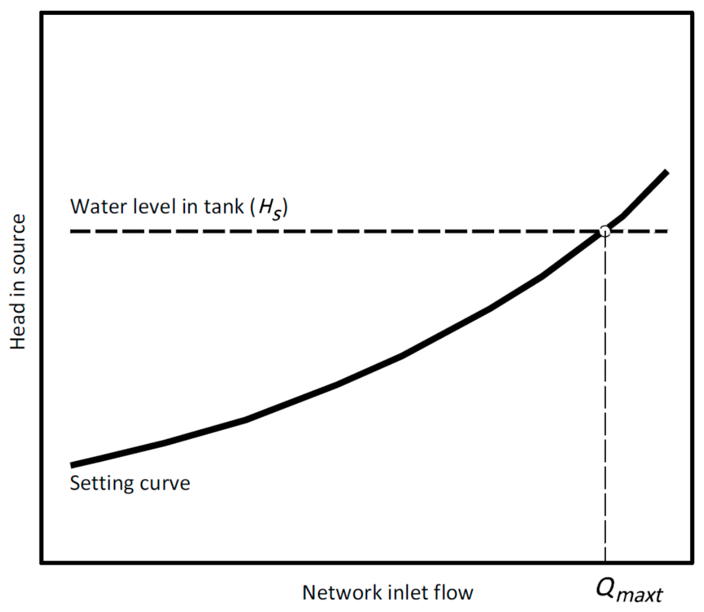
2.3. Theoretical Maximum Flow

The theoretical maximum flow, Q_maxt, or network capacity defines the maximum flow that a network can supply with at least a minimum pressure, P_min, at every node. The lowest pressure node must have the predefined minimum pressure [30]. The theoretical maximum flow value is determined through a demand-driven-analysis (DDA) hydraulic modeling of the network, in which nodes are associated with a given average demand. For this determination, several working conditions are evaluated and the peak factor is modified until the minimum pressure at the most unfavorable network node is guaranteed.

For this purpose, a setting curve—a network-H-Q curve that guarantees the minimum pressure at the lowest pressure node—is used. In a tank supplied network, for example, (see Figure 1), the intersection between the setting curve and the source water level determines the theoretical maximum flow. If due to minimum pressure reduction, the setting curve runs lower, then network capacity is increased.

2.4. Sector Development

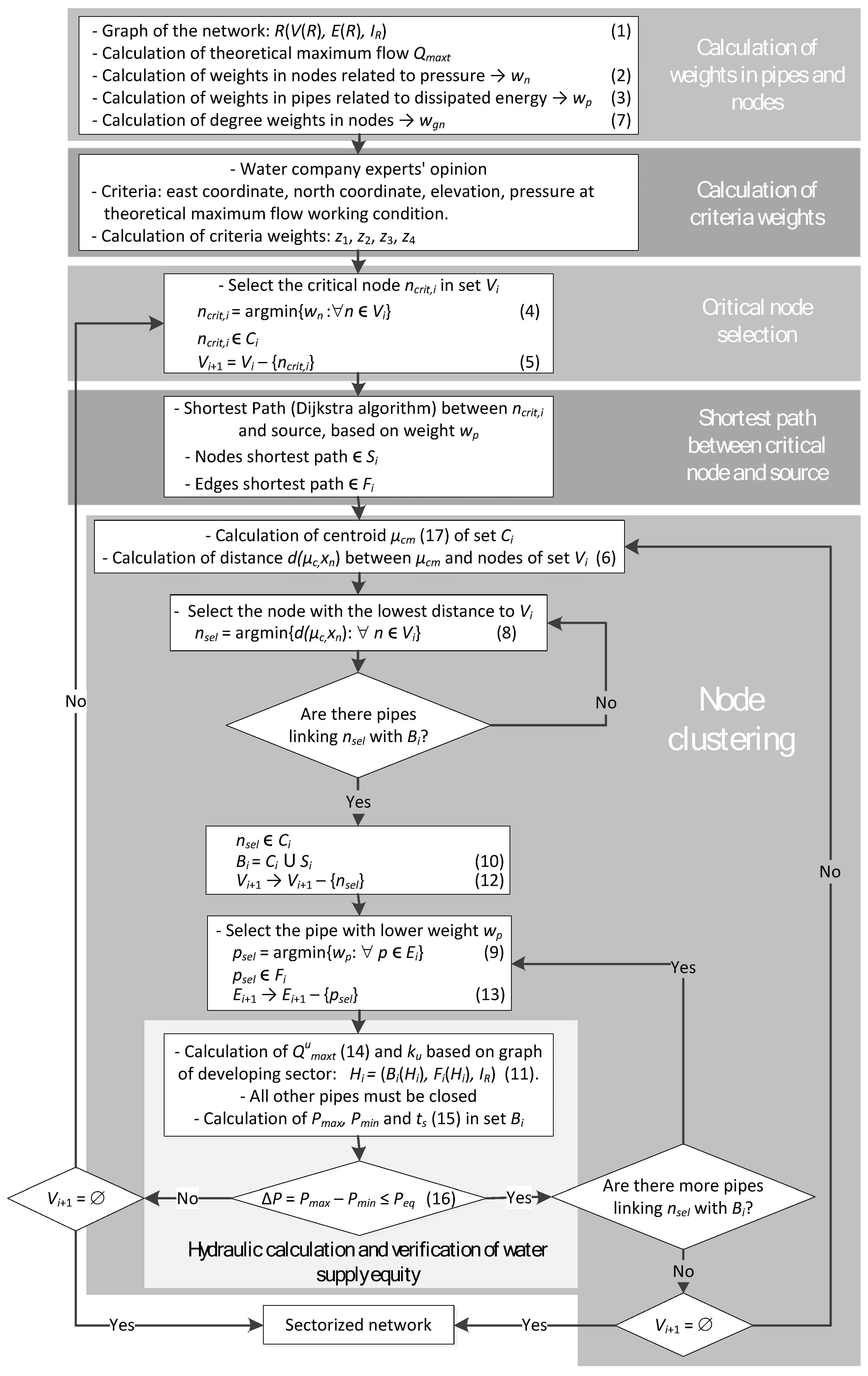
Our sectorization process, which is fully described in this subsection, is schematized in Figure 2. This figure must be understood as a high-level pseudocode, with appropriate references to the equations in this subsection, accompanied by conceptual descriptions for the various sub-processes that integrate the entire process and which are described in detail below. These sub-processes are:

• Calculation of weights in pipes and nodes
• Calculation of criteria weights
• Critical node selection
• Shortest path between critical node and source
• Node clustering
• Hydraulic calculation and verification of water supply equity

For the stages that require hydraulic calculation we use EPANET 2.0 [41].

To better follow this subsection,

Table 1. List of used variables.

Variable	Definition	Unit
R	Graph of whole network, used as hydraulic model	-
V(R)	Set of whole network nodes	-
E(R)	Set of whole network pipes	-
$I_R$	Incidence relation of graph	-
Qmaxt	Theoretical maximum flow or network capacity	L/s
n	Node	-
p	Pipe	-
$P_n^{Qmaxt}$	Pressure at nodes at theoretical maximum flow working condition	m
$Q_p^{Qmaxt}$	Flow at pipes at theoretical maximum flow working condition	L/s
$h_p^{Qmaxt}$	Head loss at pipes at theoretical maximum flow working condition	m
wn	Weight in node n	m
wp	Weight in pipe p	m-1
z1	Weight for east coordinate criterion	-
z2	Weight for north coordinate criterion	-
z3	Weight for elevation criterion	-
z4	Weight for service pressure criterion	-
ncrit,i	Critical node at the developing sector i	-
i	Developing sector	-
Ci	Subset of selected nodes or developing sector	-
Vi	Set of remaining nodes	-
Ei	Set of remaining pipes	-
Si	Subset of shortest path nodes	-
Fi	Subset of shortest path pipes	-
d(µc,xj)	Similarity distance	-
m	Number of criteria weight, m = 1 for east coordinate, m = 2 for north coordinate, m = 3 for elevation, and m = 4 for service pressure	-
µcm	Centroid depending on the m criteria	-
xnm	Normalized value for each n node, depending on the m criteria	-
gn	Node degree	-
wgn	Weight for node degree	-
M	Constant depending on the node degree importance	-
nsel	Selected node	-
psel	Selected pipe	-
q	Node of subset Ci	-
xqm	Normalized value for each q node, depending on the m criteria	-
Bi	Node subset used for hydraulic calculations	-
Nc	Total node number of a sector	-
Hi	Graph of developing sector i, used as hydraulic model	-
u	Working condition for developing sector	-
$Q_{maxt}^u$	Theoretical maximum flow for working condition u	L/s
ku	Peak factor for working condition u	-
Pmin	Minimum pressure in subset Bi	m
Pmax	Maximum pressure in subset Bi	m
j	Node of subset Bi	-
Qj	Average demand for each j node in subset Bi	L/s
ns	Total node number of subset Bi	-
ts	Supply time	h
Vs	Total supplied water volume in continuous and intermittent supply	m3
ΔP	Pressure difference	m
Peq	Limit value of pressure difference that assures water supply equity	m
tmin	Minimum supply time, depending on the network capacity	h
Qint	Average flow in intermittent water supply	L/s
Hs	Water level in tank or supply source	m

provides a list of the variables used.

2.4.1. Calculation of Weights in Pipes and Nodes

The network is represented by a graph R, which consists of a triplet, namely, the network node set V(R), the set of network pipes E(R), and the incidence relation $I_R$, which relates each element (edge) in E(R) to a unique non-ordered pair of nodes (vertices) in V(R):

$$R=\left(V\left(R\right),E\left(R\right),I_R\right).$$

(1)

Based on this network, we can determine the initial theoretical maximum flow, Q_maxt, as described above (see [30] for specific details). Pipes are subjected to their maximum to fulfill the minimum pressure requirements. The calculated pressure, $P_n^{Qmaxt}$, at each node n; and the obtained flow, $Q_p^{Qmaxt}$, and head loss, $h_p^{Qmaxt}$ for each pipe p, are used in weight calculation as follows.

Node weights, w_n, are directly related to the pressure at each node n:

$$w_n=P_n^{\mathit{Qmaxt}}.$$

(2)

Under the same working condition, a pipe weight, w_p, is determined by the inverse of the power dissipation [42], a function of the water specific weight, γ, and the calculated flow and head loss on pipe p, as in (3).

$$w_p=\frac{1}{\gamma \cdot \left|Q_p^{Qmaxt}\right|\cdot h_p^{Qmaxt}}.$$

(3)

With the pipe weights, the network becomes an undirected weighted graph, in which it is possible to recognize least-loss-energy pipes.

At this stage, using the graph of the entire network, we also calculate the degree of each node, g_n, which is later used to determine the degree weight, w_gn, and the similarity distance (see below).

2.4.2. Calculation of Criteria Weights

In the process, for node selection and subsequent sector development, various node-related criteria are considered, namely: east coordinate; north coordinate; elevation; pressure at theoretical maximum flow working condition; and connection degree.

Criteria weights, z_m, (m = 1 for east coordinate, m = 2 for north coordinate, m = 3 for elevation, and m = 4 for service pressure) are derived from the opinion of the water company experts, since they are fully acquainted with the network characteristics and performance. To derive those weights we use pairwise comparison matrices and their Perron eigenvectors to transform opinions into weights or priorities, as in the analytic hierarchy process (AHP) [43,44]. A different treatment is given to the connection degree, as explained below.

2.4.3. Critical Node Selection

This is an iteration process starting after completing the initialization stages 2.4.1 and 2.4.2. In each iteration step, first an individual (a node) for building the next cluster is identified. Some individuals are then grouped around it, and clusters (sectors or DMAs) are thus defined iteratively.

To build the i-th sector, we first identify the critical network node, n_crit,i, in the set of remaining nodes, V_i (initially, all the nodes of the entire network belong to this set). This critical node is selected to be the least-supply-pressure node during the maximal theoretical flow working condition, according to (2):

$$n_{crit,i}=\arg \min \left\{w_n:\forall n\in V_i\right\}.$$

(4)

This node is also the seed element of cluster C_i under development. Thus, it is the first element in cluster C_i, and must be included in this set: n_crit,i ϵ C_i.

Moreover, to avoid further selecting the critical node from the next set, V_i+1, it must be removed from the previous set, V_i:

$$V_{i+1}=V_i-\left\{n_{crit,i}\right\}.$$

(5)

2.4.4. Shortest Path between Critical Node and Source

With the dissipation energy weight, w_p, of every pipe, the critical node as a start, and the supply source as a destination, we determine the shortest path between both using the Dijkstra algorithm [45]. If there is more than one supply source, the shortest path must be determined for all sources. This step is essential to identify sectors, since each sector will have its own starting shortest path. Due to pipe weight characteristics, the shortest path will usually be made up of larger diameter pipes.

This path is used for hydraulic calculations as a sector entrance. A second node subset, S_i, which groups shortest path nodes, is also defined, as well as a pipe subset, F_i, which groups the shortest path pipes.

2.4.5. Node Clustering

The critical node becomes the cluster initial centroid, µ_c, (see (17) below for an exemption) and the next node is selected from subset V_i. This selection is determined by using the similarity distance,

$$d\left({\mu }_c,x_n\right)=w_{gn}\cdot \sqrt{{\displaystyle \sum _{m=1}^4{z}_m\cdot {\left({\mu }_{cm}-x_{nm}\right)}^2}},$$

(6)

between centroid µ_cm and normalized value x_nm for each node n, depending on the m criteria, and on the cluster connection through an edge (pipe). Before stating the selection mechanism, we first explain (6) further.

The weight w_gn is described below. Note that normalization for each criterion is performed by dividing each value by the sum of the criterion values.

Using east and north coordinates, we determine an equivalent value to the horizontal distance between the centroid and every network node. Closer nodes to the centroid are more likely to be grouped in the forming cluster. Normalization of these coordinates must refer to a common value to avoid modifying scales of the reference plane axes. This common value may be the greatest value of the east or north coordinates sum.

Node elevation and pressure criteria are particularly useful to achieve equity in sector supply. In this way, clusters are integrated by nodes with similar pressure and elevation.

This selection process may leave isolated nodes that connect with a sector through a single pipe and are unable to form a new sector. For this reason, similarity distance (6) is calculated using a weight, w_gn, which depends on the degree, g_n, of node n in the network. Nodes with a low connection degree are prioritized in the selection by means of

$$w_{gn}=1+\frac{g_n}{M}.$$

(7)

M is a constant that depends on the importance of the node degree. Assuming low values for M (1 to 10) implies giving more importance to the node connection degree in the network. Low values are recommended for branched networks, in which branches are in an unfavorable location (distant nodes or nodes with differing elevations or pressures). In the case of looped networks with uniform characteristics, M may be greater (50 to 100), and a value w_gn = 1 may be adopted. Prioritizing low connection degree nodes may increase pressure differences between the highest and lowest pressure nodes in the cluster. Consequently, smaller sectors are created.

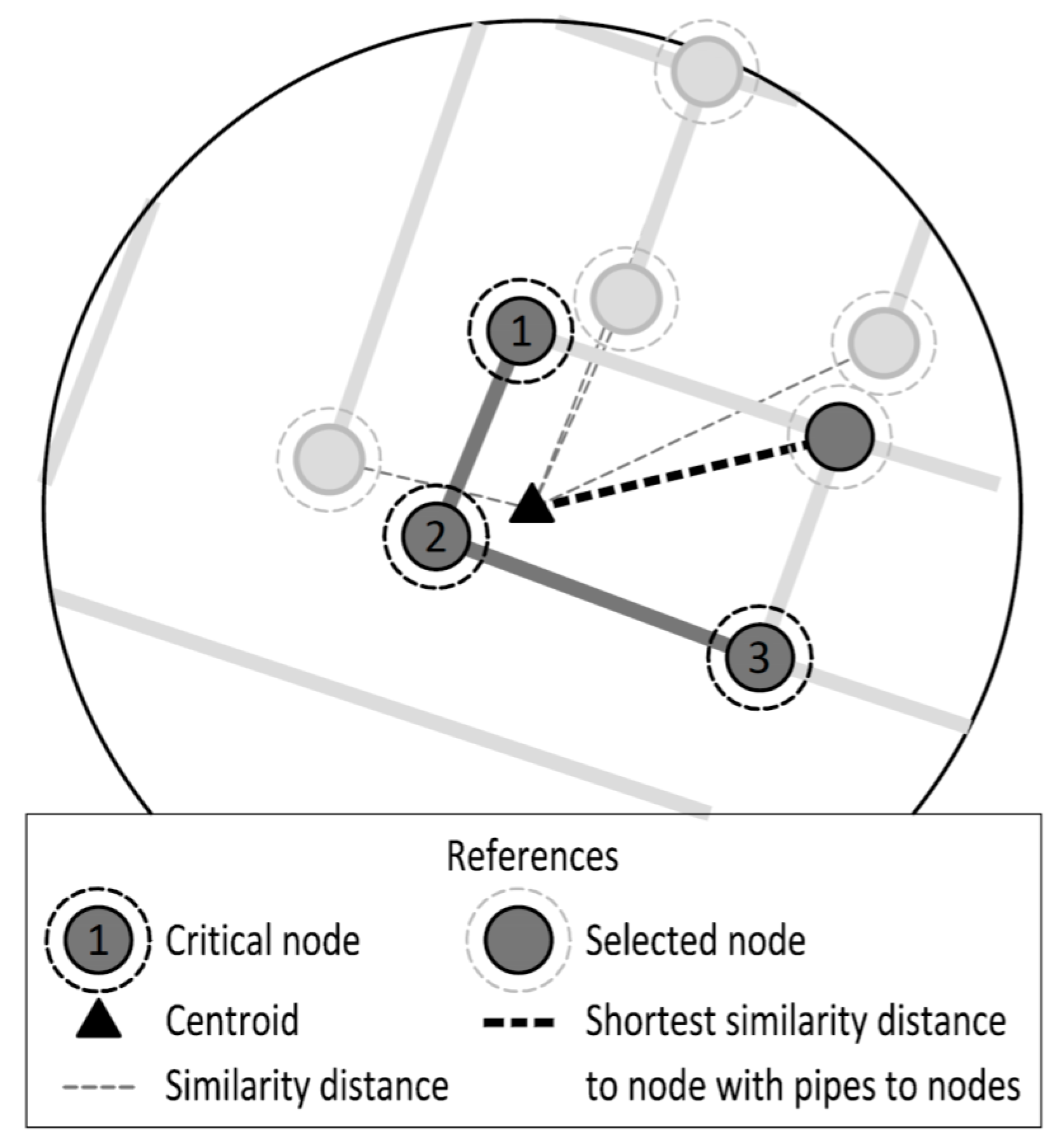
To select the next node to belong to the cluster, we consider the graph used in the hydraulic calculation. The selected node, n_sel, is the graph node minimizing (6), that is to say, the graph node with the smallest similarity distance:

$$n_{sel}=\arg \min \left\{d({\mu }_c,x_n):\forall n\in V_i\right\}.$$

(8)

However, we also need to guarantee the existence of an edge between the previously selected nodes, and the newly selected node (Figure 3). As a result, to select a node we need more than one iteration.

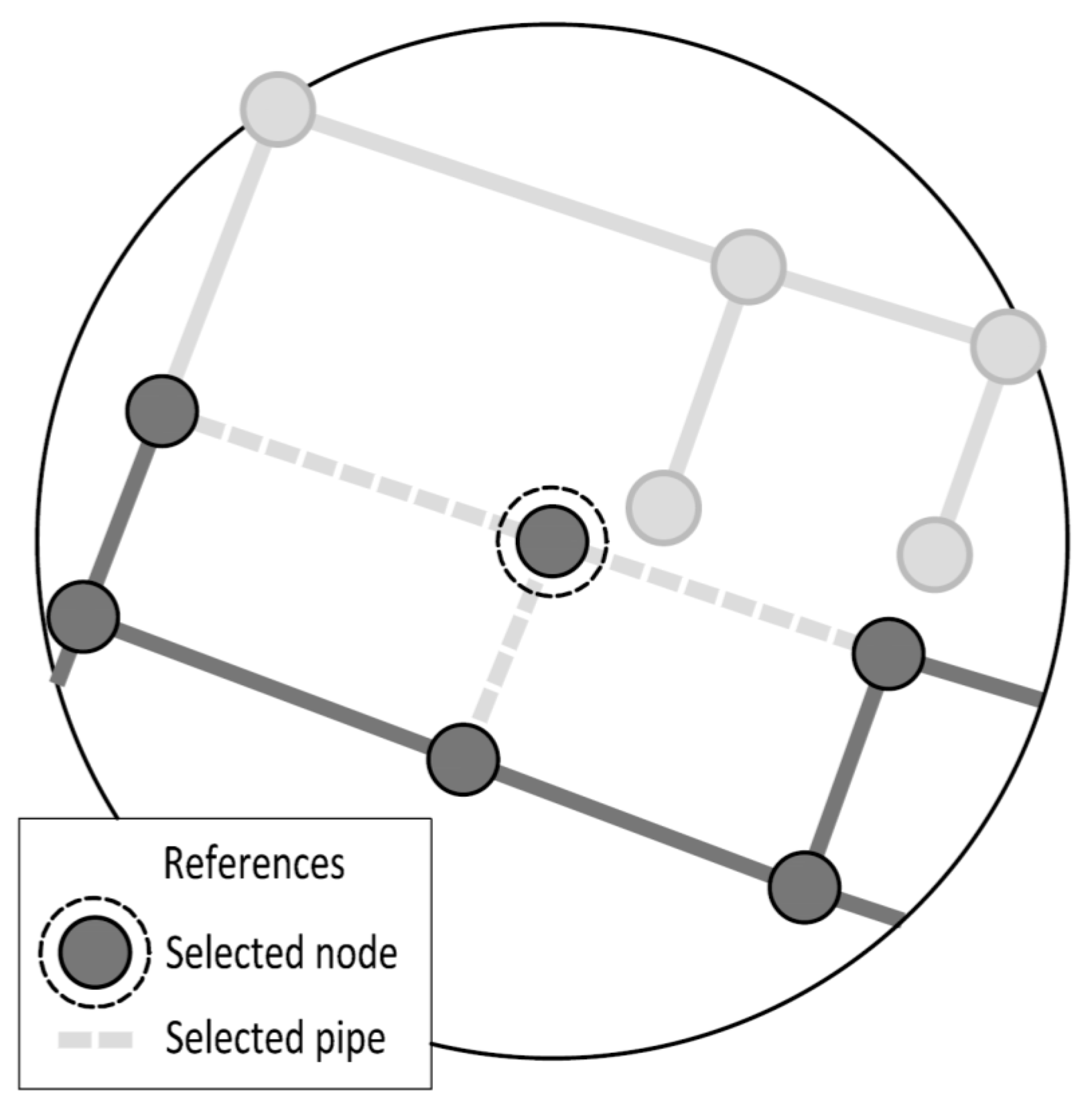
If a new selected node has many pipes connecting with the sector (Figure 4), then the water has many options to flow and sector capacity is likely to increase.

Conversely, if the selected node has few links with the new sector, reducing pressure loss by changing the number of available circulation routes is less likely to succeed. Increasing or decreasing the network capacity and achieving the desired equity depends on the elevation and pressure of the selected node. If a node has a comparatively low elevation in the sector, it has a high pressure. Thus, this node may become the highest pressure node, which reduces equity and defines the further selection process. If a node has a higher elevation than the elevation node average, it may become a new critical node due to its minimum pressure, whose effect tends to reduce sector capacity.

By selecting the smaller diameter pipes first, the selected pipe, p_sel, from the set of current available pipes, E_i, is the pipe with lowest weight w_p:

$$p_{sel}=\arg \min \left\{w_p:\forall p\in E_i\right\}.$$

(9)

Every selected node, n_sel, and pipe, p_sel, must be included in the developing cluster, C_i (n_sel ϵ C_i) and in the shortest path pipe subset, F_i, (p_sel ϵ F_i), respectively. Moreover, the subset of the critical path nodes, S_i, must also join the cluster node subset, C_i, to obtain node subset B_i, as in (10), which is the base for the new graph, H_i, as specified in (11). This graph is used for hydraulic calculations.

$$B_i=C_i\cup S_i,$$

(10)

$$H_i=\left(B_i\left(H_i\right),F_i\left(H_i\right),I_R\right).$$

(11)

To avoid picking more than once any nodes and pipes previously selected for other sectors, each must be removed respectively from the new vertex set, V_i+1, and edge set, E_i+1, used in the next iteration:

$$V_{i+1}\to V_{i+1}-\left\{n_{sel}\right\},$$

(12)

$$E_{i+1}\to E_{i+1}-\left\{p_{sel}\right\}.$$

(13)

Now it is time for hydraulic calculations with the current sector B_i.

2.4.6. Hydraulic Calculation and Verification of Water Supply Equity

At the beginning of the hydraulic calculations, only pipes in subset F_i are considered open, while the remaining pipes are considered closed until a node that connects them to the developing sector is selected. This situation may have a huge influence in the sector capacity calculation and, consequently, in equity and supply times.

We now calculate the theoretical maximum flow, $Q_{maxt}^u$, with the graph of the developing sector H_i for a working condition u. We also determine the maximum, P_max, and the minimum, P_min, pressures for the selected set of nodes, B_i. Thus, we are able to determine the peak factor, k_u, and, using the average demand, Q_j, for any selected node j, j = 1, …, ns, we obtain for this working condition

$$Q_{\mathit{maxt}}^u=k_u\cdot {\displaystyle \sum _{j=1}^{ns}{Q}_j}.$$

(14)

To determine the supply time, t_s, we assume that the consumed water volume in continuous supply equals that of intermittent supply, $V_s={\displaystyle \sum _{j=1}^{ns}{Q}_j\cdot 24}=Q_{\mathit{max}t}^h\cdot t_s$. Furthermore, we consider that the average flow is distributed 24 h a day, and the network capacity [30] is high enough to supply a high flow, $Q_{maxt}^u$, in a short supply time. Thus,

$$t_s=\frac{24}{k_u}.$$

(15)

Usually, the greater the number of grouped nodes, the lower the peak factor k_u value, so supply periods tend to 24 h. If the number of nodes is low, the peak factor increases, and thus supply time is shorter. In this case, having fewer supply hours is useful for avoiding supply schedule overlap.

The configuration and number of nodes in a hydraulic sector limits its theoretical maximum flow and, thus, its peak factor as well. Consequently, there is an intrinsic relation between a sector size and its supply time to guarantee an appropriate pressure.

The process of cluster selection of nodes comes to an end when the pressure difference, ΔP, of the hydraulic calculations surpasses a limit value, P_eq, which assures water supply equity:

$$\mathrm{\Delta }P=P_{max}-P_{min}>P_{eq}.$$

(16)

If the pressure difference, ΔP, still guarantees equitable supply, perhaps new elements (nodes and pipes) can be incorporated in the current sector. To this end, if there are still unassigned nodes (V_i is not empty) a new centroid, µ_cm, is determined for each criterion m. We use the normalized values x_qm for each node q, which makes up the developing sector B_i, N_c being its total number of nodes:

$${\mu }_{cm}=\frac{1}{N_c}{\displaystyle \sum _{q=1}^{N_c}{x}_{qm}}.$$

(17)

If, on the other hand, P_eq is effectively surpassed and there are still unassigned nodes (V_i is not empty), we start the iteration process in Section 2.4.3 again, and use the next critical network node, which is selected from all the excluded nodes (already grouped in previous clusters). From this new critical node, a new sector is built. Each network sector is built this way until all the nodes are assigned to a sector. This ends the sectorization process.

3. Case Study Description

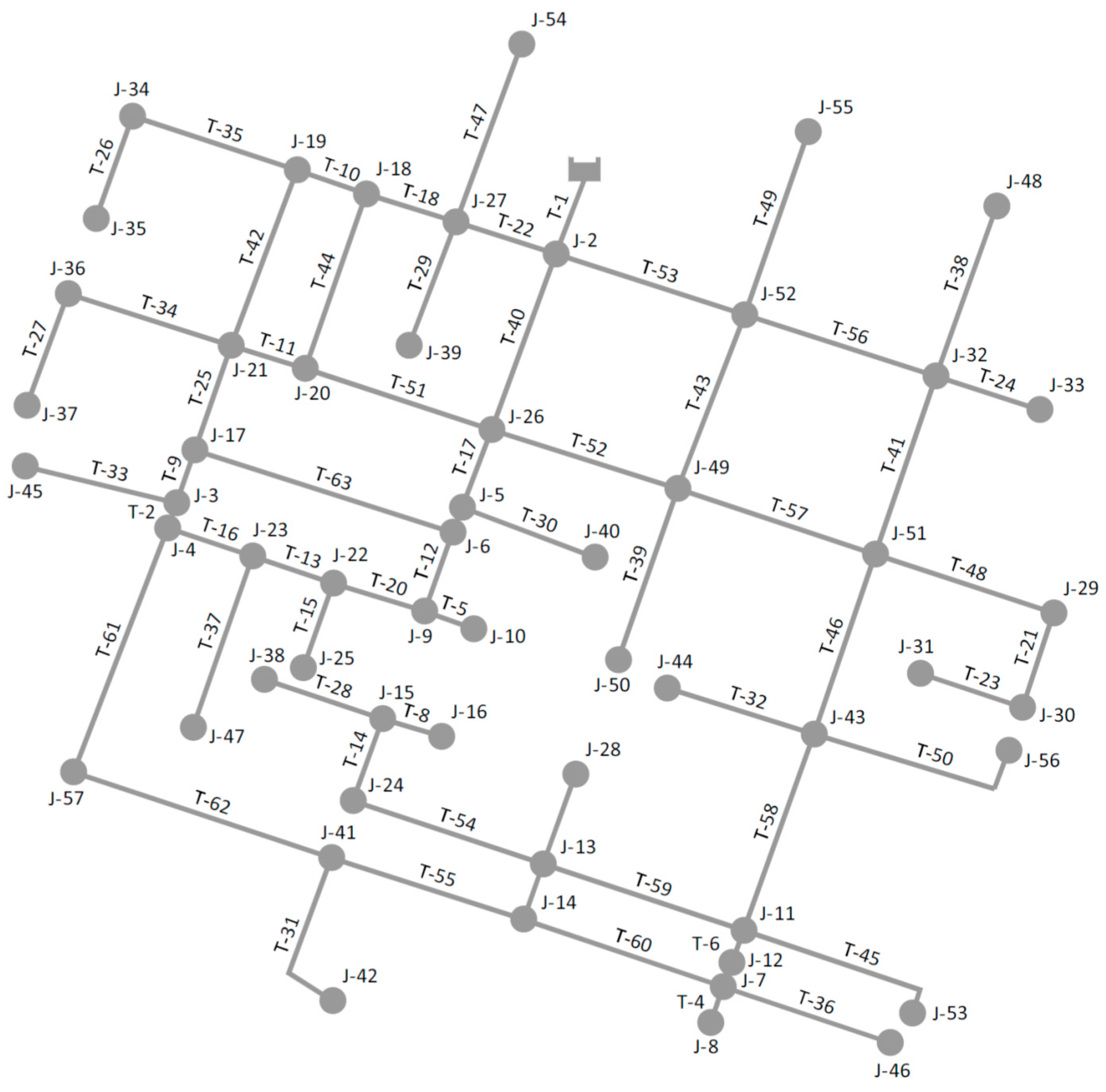
The case-study network, shown in Figure 5 and summarized in

Table 2. Main network characteristics of the case study.

Description	Value
Number of network nodes	56 nodes
Number of network pipes	61 pipes
Average demand flow in intermittent water supply	12.64 L/s
Current supply time	4 h
Minimum pressure	5.30 m
Maximum pressure	17.20 m

, corresponds to a subsystem of the water supply network of Oruro (Bolivia). This network is supplied for 4 h a day, its demand flow during this period is 12.64 L/s, and its minimum pressure is 5.30 m. The minimum water level at its source is 3737 masl (meters above sea level), and the network average elevation is 3718 masl.

To achieve an equitable supply and build large sectors, we adopt a minimum pressure of 10 m and a pressure difference of 5 m, which is the maximum value recommended by CPHEEO.

Preliminary Evaluation of Water Supply Equity

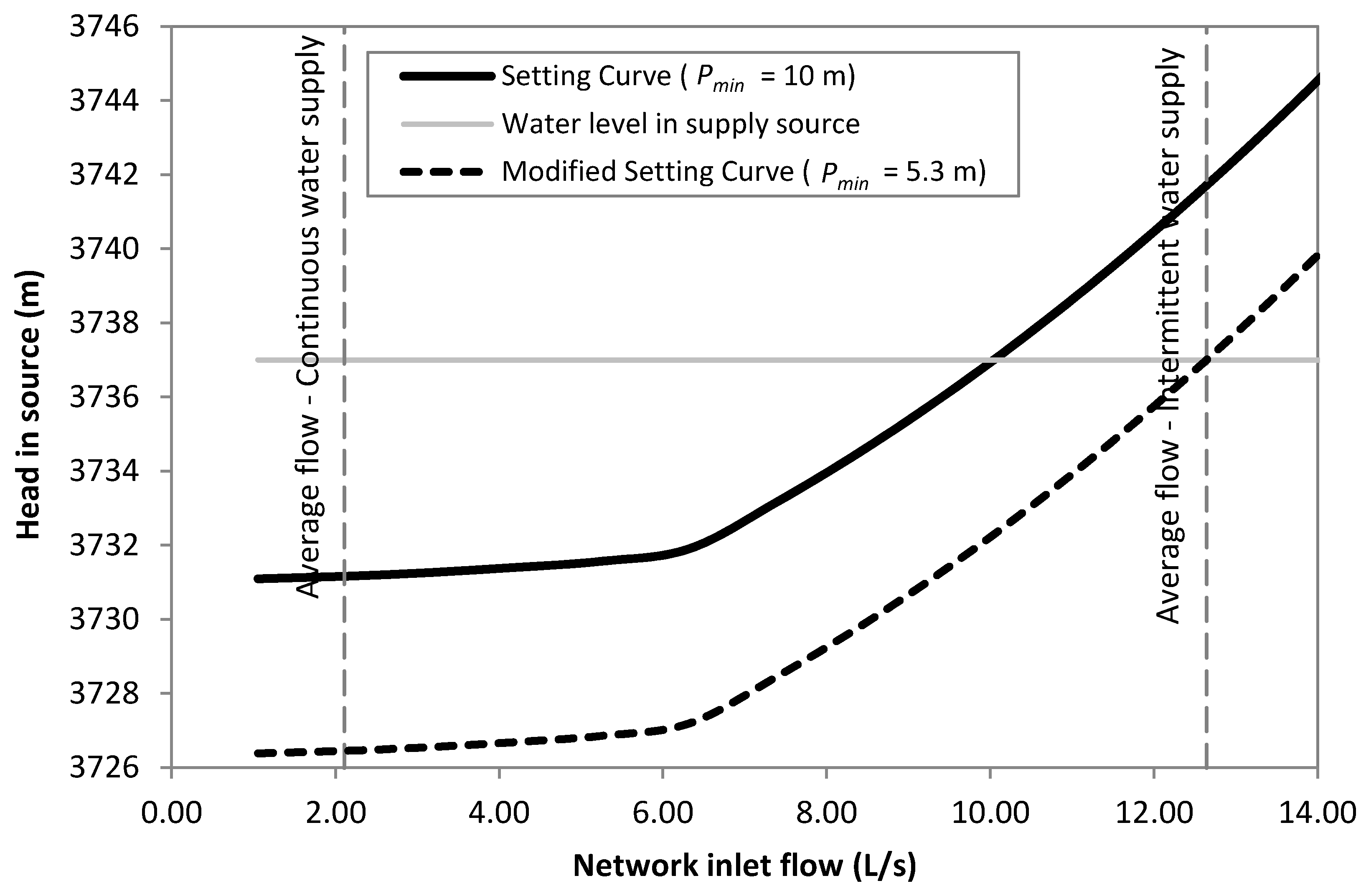
Before applying our process, we evaluate some modifications in the current network management to try to achieve equitable supply. First, we determine the setting curve and network maximum theoretical flow [30] that satisfies the minimum service pressure of 10 m (Figure 6). The theoretical maximum flow or network capacity is 10.04 L/s, which does not fulfill the population demand in intermittent supply (12.64 L/s). One way to satisfy this requirement is by reducing the minimum service pressure to P_min = 5.30 m, which rearranges the setting curve to a fulfillment of the demanded flow (Figure 6).

As a result, the minimum pressure (10 m) is not met. Moreover, the difference in pressure ΔP = 11.99 m between the maximum pressure 17.29 m and the minimum pressure 5.30 m far exceeds the desired pressure of 5 m. Thus, other solutions must be evaluated.

A second alternative is increasing the number of supply hours (18). In this way, we reduce the average flow in intermittent supply (Q_int = 12.64 L/s) to a value that equals the current network capacity (Q_maxt = 10.04 L/s), using

$$t_{\mathit{min}}=\frac{t_s\cdot Q_{int}}{Q_{\mathit{maxt}}}.$$

(18)

If we modify the initial supply time, t_s = 4 h, to a minimum supply time, t_min = 5.04 h, the demand is satisfied by the network capacity, 10.04 L/s, and the pressure at each node is over 10 m. Nevertheless, we must also evaluate pressure differences. We determined the pressure difference ΔP = 7.88 m between the maximum pressure 17.88 m and the minimum pressure 10.00 m, which clearly exceeds 5 m and thus equity is not guaranteed.

As a consequence, a sectorization alternative needs to be studied. In the next section, we apply the process developed in this paper.

4. Results and Discussion

As shown, for the sectorization process, we use the following criteria: east coordinate; north coordinate; elevation; pressure; and node degree (

Table 3. Criteria for clustering process.

Node	East Coordinate (m)	North Coordinate (m)	Elevation (m)	Pressure (m)	Degree
J-2	698,074.22	8,010,604.23	3719.00	17.87	4
J-3	697,855.66	8,010,454.61	3719.00	16.05	3
J-4	697,853.41	8,010,448.53	3718.98	16.06	3
⋮	⋮	⋮	⋮	⋮	⋮
J-57	697,801.55	8,010,310.70	3718.60	13.14	2
Sum	-	448,583,649.73	208,217.36	808.56	-

). All except the node degree, need to be normalized (

Table 4. Normalized values.

Node	xn1	xn2	xn3	xn4
J-2	0.00155617	0.01785755	0.01786114	0.02210271
J-3	0.00155569	0.01785721	0.01786115	0.01984983
J-4	0.00155568	0.01785720	0.01786103	0.01985699
⋮	⋮	⋮	⋮	⋮
J-57	0.00155557	0.01785689	0.01785921	0.01625678

).

Criteria weights are determined based on interviews with water company experts. In this case, study, three company experts were interviewed. Thus, we set pairwise comparison matrices [44] that influence every criterion (except for node degree, which, as explained above, receives a different treatment). Perron eigenvectors represent the criteria weights that were defined by the company experts.

Table 5. Pairwise comparison matrix, expert 1.

Criterion	East and North Coordinates	Elevation	Pressure	Eigenvector
East and north coordinates	1	3	1/2	0.333
Elevation	1/3	1	1/3	0.140
Pressure	2	3	1	0.528

shows the pairwise comparison matrix of expert 1 as well as its Perron eigenvector. These values have a consistency ratio (CR) of 5.1%, which is suitable for the criteria [44]. The final weights are obtained through the component geometric from the Perron eigenvectors for the experts (

Table 6. Normalized weight of each criterion.

Criterion	Expert 1	Expert 2	Expert 3	Geometric Mean	Normalized Weight
East and north coordinates	0.333	0.333	0.200	0.281	z1 = z2 = 0.291
Elevation	0.140	0.333	0.200	0.210	z3 = 0.218
Pressure	0.528	0.333	0.600	0.473	z4 = 0.490
Total	1	1	1	0.964	1

), which also had acceptable CR values.

Due to the network characteristics, it is less likely that disconnected nodes are left during sector building. Therefore, as discussed above, taking (7) into account, we assume a weight w_g = 1 for each node.

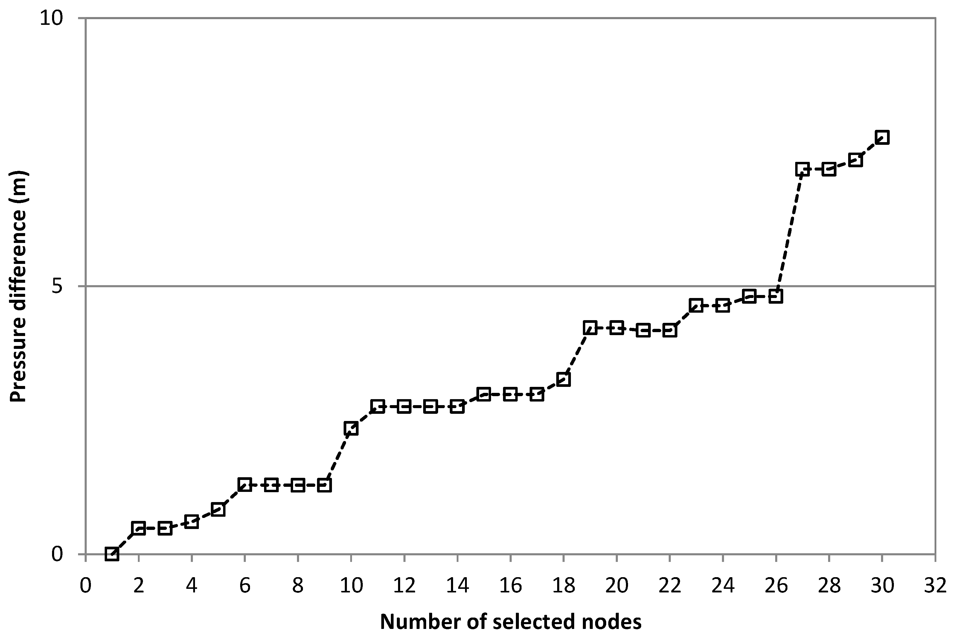
To start building the first sector, we identify node J-38 as the most critical node in the network. Starting from this node, we determine the shortest path to its supply source (see Figure 11, which compiles the final results), and thus we set the first sector. Later, we group nodes according to their similarity distance. Every step is evaluated until each node has a pressure difference that assures the desired equity (Figure 7).

The clustering process produces evident jumps in pressure differences (Figure 7), due to selection of nodes that enable either raising the pressure, or reducing the minimum pressure. After surpassing the pressure difference of 5 m, DMA implementation stops, and according to this condition, the first 26 nodes selected make up the first sector, without considering the first nodes of the identified shortest path (see Figure 11).

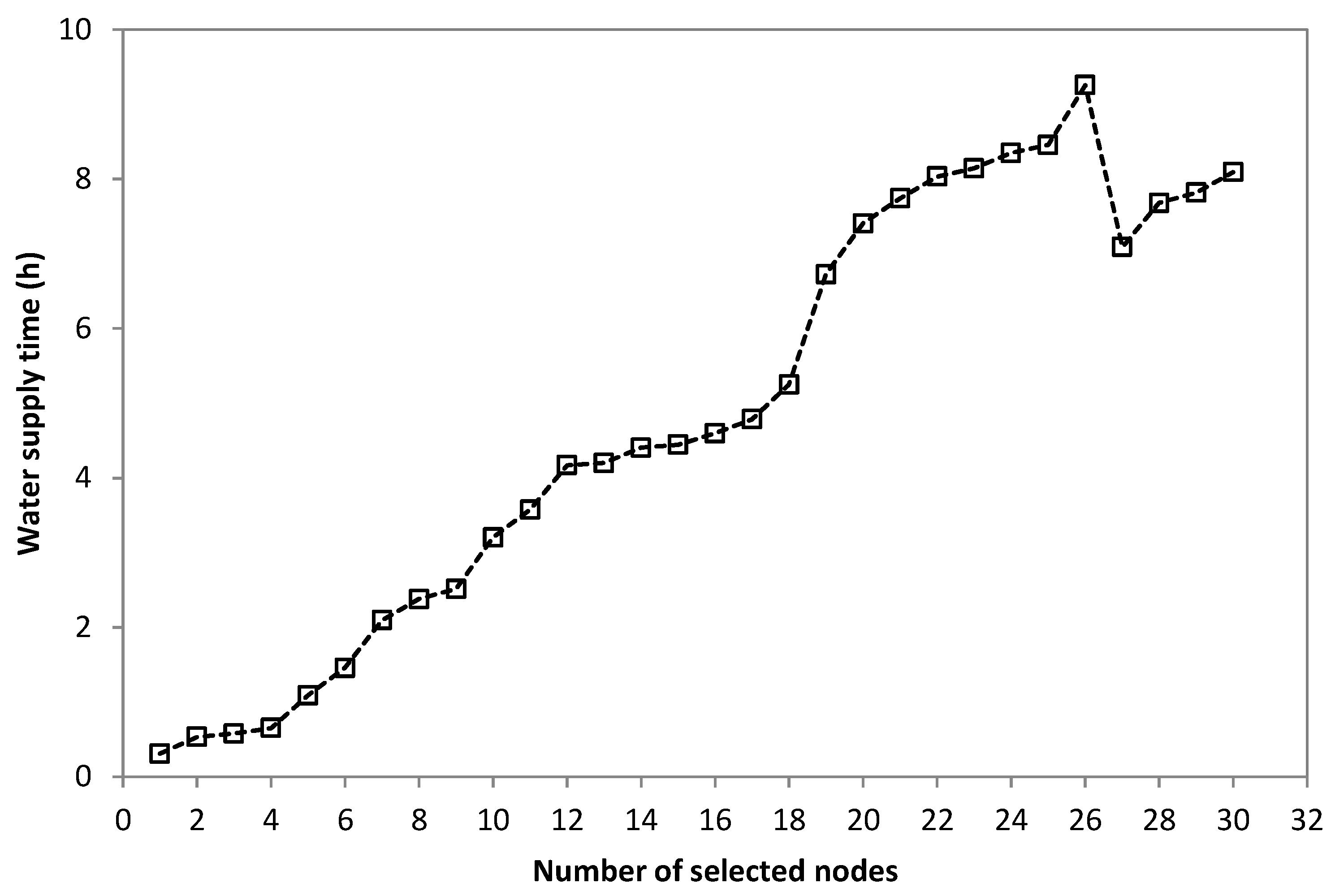
The sudden increase in the developing sector capacity is caused by selecting nodes that have a high degree of connection. This situation causes a reduction in supply time, because the greater the capacity, the shorter the supply time (Figure 8).

Let us continue with the process. The network critical node has already been selected for the first sector. Consequently, there is a new critical node among the unselected nodes. Since pressure difference between this node and the supply source is large, an equitable supply is difficult to achieve. Consequently, we consider reducing the head in the source, or creating more sectors. For better network performance, in terms of supply equity, and to reduce leaks, it is better to reduce the head at the supply source.

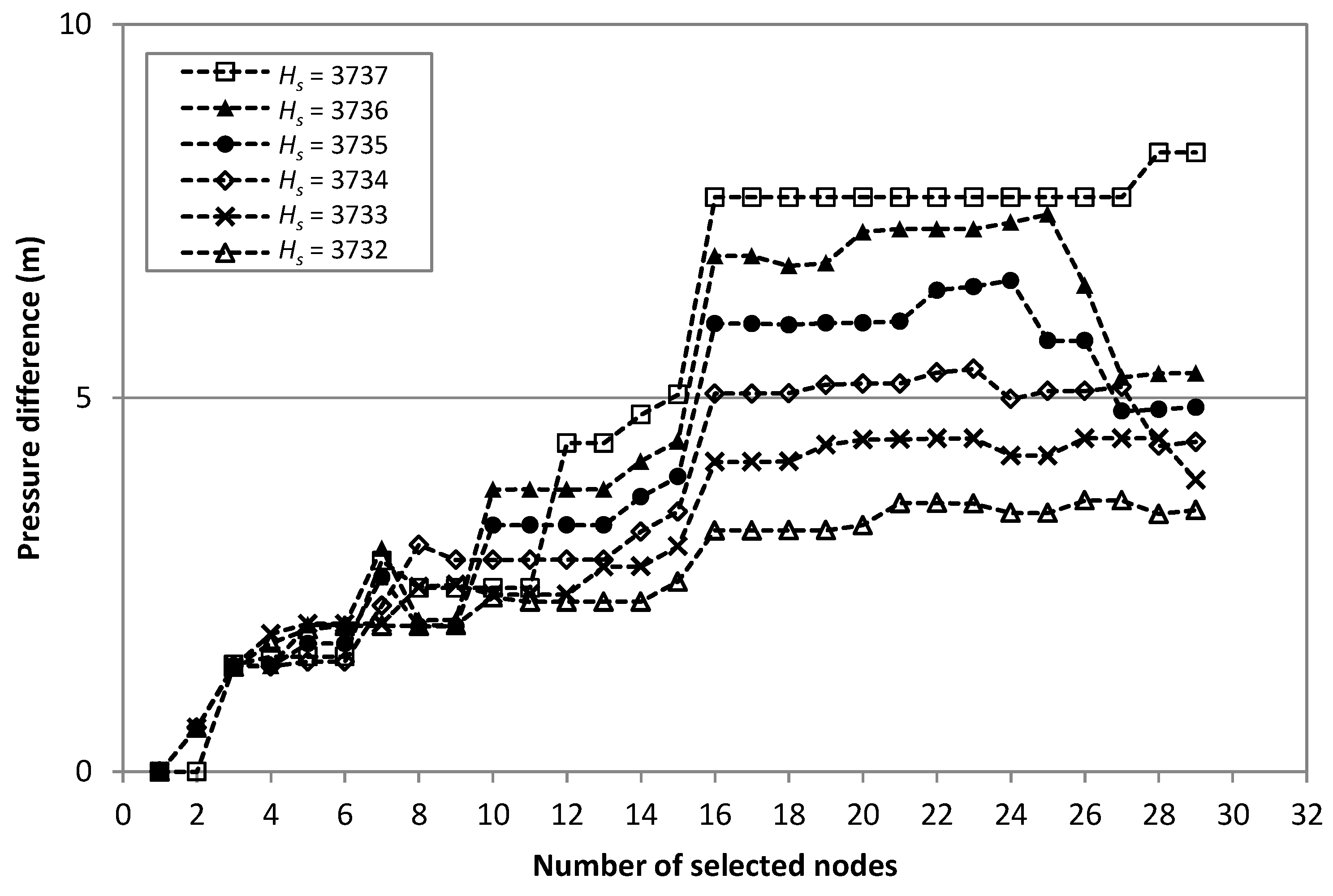
We now evaluate situations in which the head at supply source, H_s, is reduced. Moreover, we increase the pressure difference value to analyze the sector configuration behavior at high pressures (Figure 9).

If the head in the source is 3737 m or 3736 m, for which the pressure difference surpasses 5 m (Figure 9), we would need to create more additional sectors. This becomes necessary because pressures must be adjusted to the pressure difference between the pressure at the nodes near the supply source and the lowest pressure node.

If the head in the source is reduced, we obtain pressure differences lower than 5 m starting from values lower than 3735 m. The lower the head in the source, the lower the pressure difference between the supply source and the critical node, with which we achieve a greater supply equity. Nevertheless, pressure difference reduction means increasing supply service time.

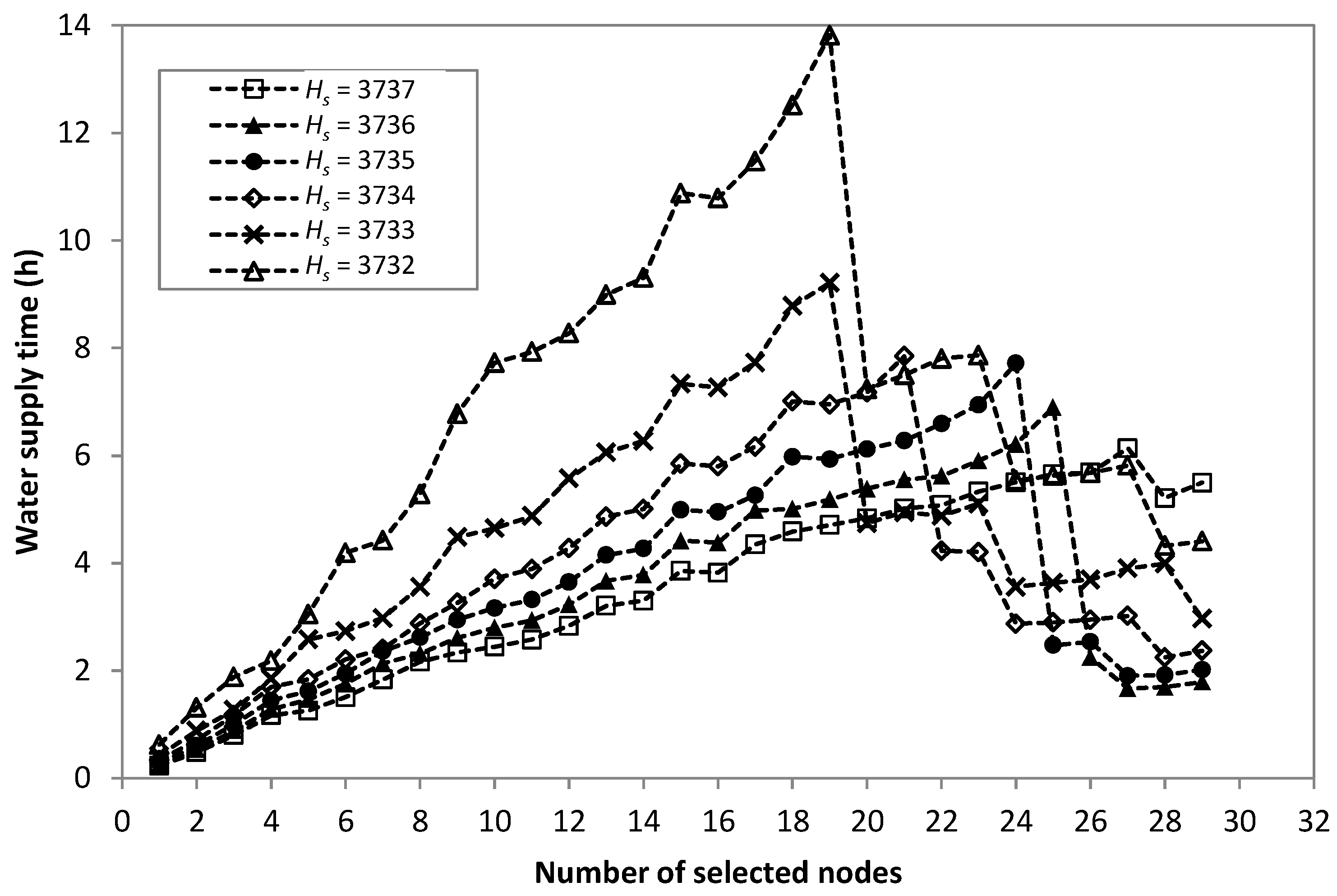
As for the first sector, sudden reductions in supply hours (Figure 10) are caused by increasing the network capacity, which, in turn, is due to the selection of high connectivity degree nodes.

It is not recommendable to reduce the current number of supply hours, because users may complain. Thus, to have a 4 h supply, we define a pressure head of H_s = 3732 m (Figure 10). Under these conditions, we create the second sector (Figure 11) and guarantee the desired equity.

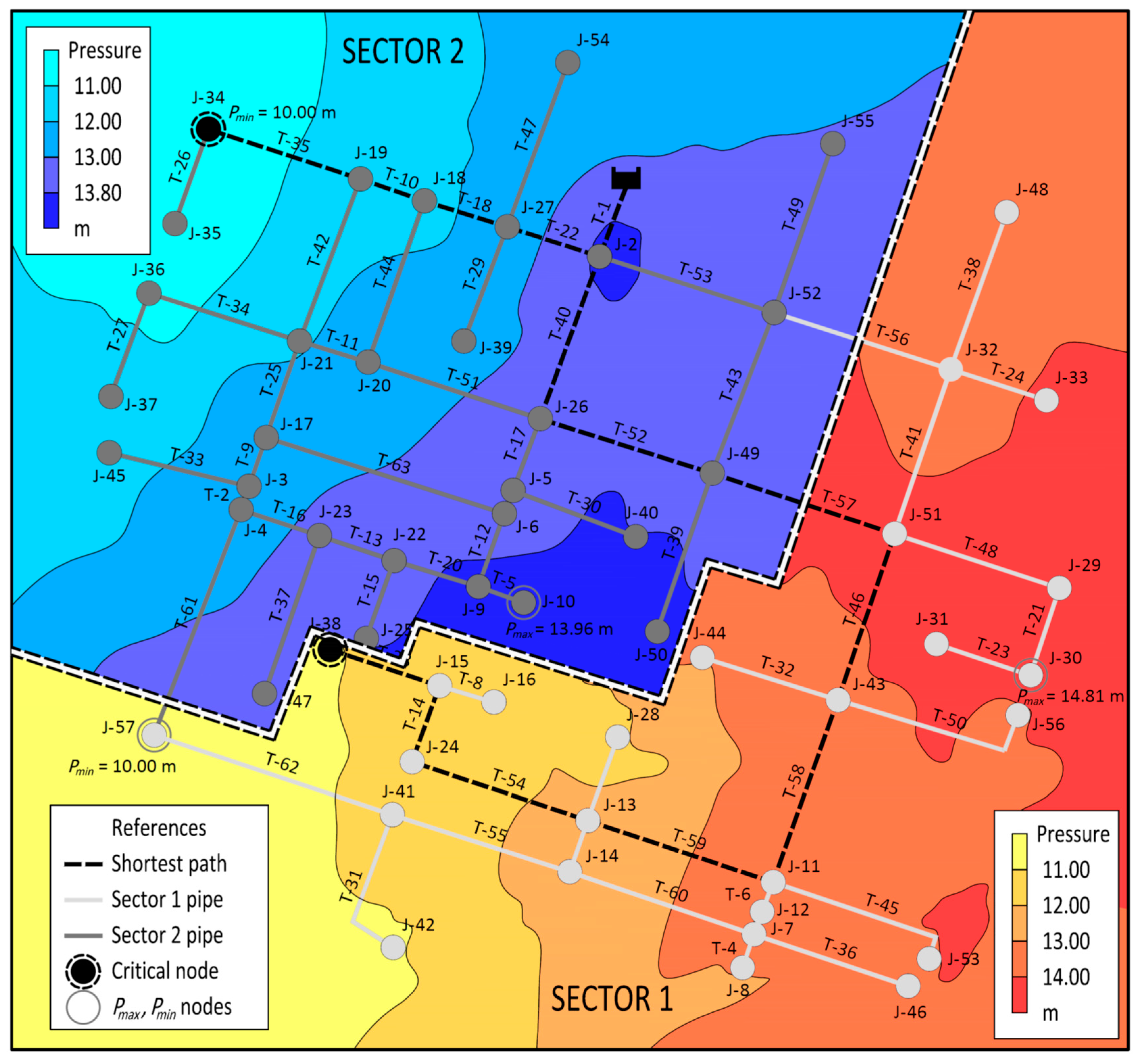
The sectorization process produces two sectors with intermittent supply (

Table 7. Characteristics of the sectors after the sectorization process.

Sector	Pmax (m)	Pmin (m)	ΔP (m)	Qmaxt (L/s)	Supply Time ts (h)	Hs (mca)	Clustering Nodes Ci
Sector 1	14.81 (J-30)	10.00 (J-57)	4.81 < 5	2.76	8.46	3737	26
Sector 2	13.54 (J-10)	10.00 (J-34)	3.54 < 5	6.18	4.41	3732	30

). The pressure difference is lower than 5 m, which assures equitable supply. We also determine the supply time based on the hydraulic characteristics of each sector.

Sector delimitation is achieved by installing sectioning valves at pipes T-56, T-22, T-53, T-51, T-17, T-39, T-43 and T-61. Pipe T-57 controls the incoming water flow to sector 1.

Due to the network characteristics, initial nodes of first shortest path, namely J-2, J-26, and J-49, work in both sectors, and supply time is longer (12.87 h). This situation could be avoided, for example, by installing a direct connection pipe between the source and sector 1.

Sector 1 includes the network critical node, which reduces its capacity and conditions the sector to have a longer supply time. Conversely, sector 2 may have greater capacity because the critical node does not belong to it, and the new critical node favors capacity increases.

5. Conclusions

In this paper, we have considered a procedure to define sectors in a water distribution network with intermittent supply. We develop sectors based on equity criteria, and using water company expert opinions. Moreover, we determine the supply time using the sector hydraulic conditions. The authors claim that these characteristics are innovative in methodologies of this kind. The developed methodology uses soft computing elements of graph theory and clustering.

The sectorization process is a very useful technical management tool for those intermittent supply systems that are unable to evolve to continuous supply, and for systems that could evolve to continuous supply.

Sector construction based on equity criteria may also be useful for a future intermittent-to-continuous-supply transition, because sectors help define areas for pressure management.

A sectorized network by itself does not guarantee equitable and predictable intermittent water supply. It is also necessary to manage the supply schedules for all sectors to avoid schedule overlaps with consequent pressure reduction [17].

In our case study, due to the network characteristics, some shortest path nodes were selected for more than one sector. This could be avoided, for example, by setting up a shortcut pipe between source and sector. However, let us note that, although these nodes are supplied for a longer period of time, they satisfy the pressure difference condition in their sector.

In larger networks with more than one supply source, we need greater computing capacity and suitable process supervision.

There are few tools for the management of intermittent supply networks. It is necessary to develop more sectorization techniques for this type of network, in which sectors are intrinsic elements. Future sectorization network research must aim at reducing the number of pipes with isolation valves, developing efficient equity indicators, and evaluating the resilience of created sectors to assure constant equity in supply.

Related to this last issue, despite the absence of explicit resilience reference values (such as for the pressure difference as recommended by CPHEEO [2]) for studies including equity as a criterion, we mention here that the resilience index [42] for the entire network is 0.894, which is, as expected, clearly improved after sectorization. In effect, the new resilience values are 0.969 for the first sector and 0.997 for the second. From our point of view, this improvement clearly backs our sectorization proposal, which we consider to be promising.

References

- World Health Organization. Constraints Affecting the Development of the Water Supply and Sanitation Sector. 2003. Available online: http://www.who.int/docstore/water_sanitation_health/wss/constraints.html (accessed on 20 July 2016).
- Central Public Health and Environmental Engineering Organisation. Manual on Operation and Maintenance of Water Supply Systems; Ministry of Urban Development; World Health Organisation: New Delhi, India, 2005.
- Dahasahasra, S.V. A model for transforming an intermittent into a 24 × 7 water supply system. Geospat. Today 2007, 8, 34–39. [Google Scholar]
- Faure, F.; Pandit, M.M. Intermittent Water Distribution. 2010. Available online: http://www.sswm.info/category/implementation-tools/water-distribution/hardware/water-distribution-networks/intermittent-w (accessed on 15 October 2017).
- Charalambous, B. The Effects of Intermittent Supply on Water Distribution Networks. Water Loss. 2012. Available online: http://www.leakssuite.com/wp-content/uploads/2012/09/2011_Charalambous.pdf (accessed on 15 October 2015).
- Knobelsdorf, J.; Mujeriego, R. Crecimiento bacteriano en las redes de distribución de agua potable: Una revisión bibliográfica. Ingeniería Del Agua 1997, 4, 17–28. [Google Scholar] [CrossRef]
- Semenza, J.C.; Roberts, L.; Henderson, A.; Bogan, J.; Rubin, C.H. Water distribution system and diarrheal disease transmission: A case study in Uzbekistan. Am. J. Trop. Med. Hyg. 1998, 59, 941–946. [Google Scholar] [CrossRef] [PubMed]
- Mermin, J.H.; Villar, R.; Carpenter, J.; Roberts, L.; Gasanova, L.; Lomakina, S.; Hutwagner, L.; Mead, P.; Ross, B.; Mintz, E. A massive epidemic of multidrug-resistant typhoid fever in Tajikistan associated with consumption of municipal water. J. Infect. Dis. 1999, 179, 1416–1422. [Google Scholar] [CrossRef] [PubMed]
- Tokajian, S.; Hashwa, F. Water quality problems associated with intermittent water supply. Water Sci. Technol. 2003, 47, 229–234. [Google Scholar] [PubMed]
- Tokajian, S.; Hashwa, F. Phenotypic and genotypic identification of Aeromonas spp. isolated from a chlorinated intermittent water distribution system in Lebanon. J. Water Health 2004, 2, 115–122. [Google Scholar] [PubMed]
- Lee, E.; Schwab, K. Deficiencies in drinking water distribution systems in developing countries. J. Water Health 2005, 3, 109–127. [Google Scholar] [PubMed]
- Kumpel, E.; Nelson, K.L. Comparing microbial water quality in an intermittent and continuous piped water supply. Water Res. 2013, 47, 5176–5188. [Google Scholar] [CrossRef] [PubMed]
- Kumpel, E.; Nelson, K.L. Mechanisms affecting water quality in an intermittent piped water supply. Environ. Sci. Technol. 2014, 48, 2766–2775. [Google Scholar] [CrossRef] [PubMed]
- Ercumen, A.; Arnold, B.F.; Kumpel, E.; Burt, Z.; Ray, I.; Nelson, K.; Colford, J.M., Jr. Upgrading a Piped Water Supply from Intermittent to Continuous Delivery and Association with Waterborne Illness: A Matched Cohort Study in Urban India. PLoS Med. 2015, 12, e1001892. [Google Scholar] [CrossRef] [PubMed]
- Vairavamoorthy, K.; Akinpelu, E.; Lin, Z.; Ali, M. Design of sustainable water distribution systems in developing countries. In Proceedings of the American Society of Civil Engineers (ASCE) Conference, Houston, TX, USA, 10–13 October 2001. [Google Scholar]
- Galaitsi, S.E.; Russell, R.; Bishara, A.; Durant, J.L.; Bogle, J.; Huber-Lee, A. Intermittent domestic water supply: A critical review and analysis of causal-consequential pathways. Water 2016, 8, 274. [Google Scholar] [CrossRef]
- Ilaya-Ayza, A.E.; Martins, C.; Campbell, E.; Izquierdo, J. Gradual transition from intermittent to continuous water supply based on multi-criteria optimization for network sector selection. J. Comput. Appl. Math. 2017, 330, 1016–1029. [Google Scholar] [CrossRef]
- Ilaya-Ayza, A.E.; Benitez, J.; Izquierdo, J.; Pérez-García, R. Multi-criteria optimization of supply schedules in intermittent water supply systems. J. Comput. Appl. Math. 2017, 309, 695–703. [Google Scholar] [CrossRef]
- Di Nardo, A.; Di Natale, M.; Santonastaso, G.; Tzatchkov, V.; Alcocer-Yamanaka, V. Water network sectorization based on a genetic algorithm and minimum dissipated power paths. Water Sci. Technol. 2013, 13, 951–957. [Google Scholar] [CrossRef]
- Ziegler, D.; Sorg, F.; Fallis, P.; Hübschen, K.; Happich, L.; Baader, J.; Trujillo, R.; Mutz, D.; Oertlé, E.; Klingel, P.; et al. Guidelines for Water Loss Reduction, A Focus on Pressure Management; Deutsche Gesellschaft für Internationale Zusammenarbeit (GIZ) GmbH and VAG Armaturen GmbH: Eschborn, Germany, 2012.
- Hajebi, S.; Temate, S.; Barrett, S.; Clarke, A.; Clarke, S. Water Distribution Network Sectorisation Using Structural Graph Partitioning and Multi-objective Optimization. Procedia Eng. 2014, 89, 1144–1151. [Google Scholar] [CrossRef]
- Farley, M. Are there alternatives to DMA? Asian Water 2010, 26, 10–16. [Google Scholar]
- Herrera, A.M. Improving Water Network Management by Efficient Division into Supply Clusters. Available online: https://riunet.upv.es/bitstream/handle/10251/11233/tesisupv3599.pdf?sequence=1 (accessed on 15 January 2017).
- Izquierdo, J.; Herrera, M.; Montalvo, I.; Pérez-García, R. Division of water supply systems into district metered areas using a multi-agent based approach. In Software and Data Technologies; Springer: Berlin/Heidelberg, Germany, 2011; pp. 167–180. [Google Scholar]
- Campbell, E.; Izquierdo, J.; Ilaya-Ayza, A.E.; Pérez-García, R.; Tavera, M. A flexible methodology to sectorize water supply networks based on social network theory concepts and on multi-objective optimization. J. Hydroinform. 2016, 18, 62–76. [Google Scholar] [CrossRef]
- Alvisi, S.; Franchini, M. A heuristic procedure for the automatic creation of district metered areas in water distribution systems. Urban Water J. 2014, 11, 137–159. [Google Scholar] [CrossRef]
- Tzatchkov, V.; Alcocer-Yamanaka, V.; Bourguett-Ortiz, V. Sectorización de redes de distribución de agua potable a través de algoritmos basados en la teoría de grafos. Tlaloc-AMH 2008, 40, 14–22. [Google Scholar]
- Di Nardo, A.; Di Natale, M.; Santonastaso, G.; Tzatchkov, V.; Alcocer-Yamanaka, V. Water network sectorization based on graph theory and energy performance indices. J. Water Resour. Plan. Manag. 2014, 140, 620–629. [Google Scholar] [CrossRef]
- McIntosh, A.C. Asian Water Supplies Reaching the Urban Poor; Asian Development Bank: Metro Manila, Philippines, 2003. [Google Scholar]
- Ilaya-Ayza, A.E.; Campbell, E.; Pérez-García, R.; Izquierdo, J. Network capacity assessment and increase in systems with intermittent water supply. Water 2016, 8, 126. [Google Scholar] [CrossRef]
- Vairavamoorthy, K.; Gorantiwar, S.D.; Pathirana, A. Managing urban water supplies in developing countries—Climate change and water scarcity scenarios. Phys. Chem. Earth A B C 2008, 33, 330–339. [Google Scholar] [CrossRef]
- Soltanjalili, M.-J.; Bozorg Haddad, O.; Mariño, M.A. Operating water distribution networks during water shortage conditions using hedging and intermittent water supply concepts. J. Water Resour. Plan. Manag. 2013, 139, 644–659. [Google Scholar] [CrossRef]
- Shrinking Glaciers Cause State-of-Emergency Drought in Bolivia. Available online: https://www.theguardian.com/environment/2016/nov/28/shrinking-glaciers-state-of-emergency-drought-bolivia (accessed on 18 January 2017).
- Jain, A.K.; Dubes, R.C. Algorithms for Clustering Data; Prentice Hall: Englewood Cliffs, NJ, USA, 1988. [Google Scholar]
- Rokach, L.; Maimon, O. Data Mining and Knowledge Discovery Handbook; Springer: New York, NY, USA, 2005; pp. 321–352. [Google Scholar]
- Fontanazza, C.M.; Freni, G.; La Loggia, G.; Notaro, V.; Puleo, V. Evaluation of the Water Scarcity Energy Cost for Users. Energies 2013, 6, 220–234. [Google Scholar] [CrossRef]
- Gottipati, P.V.; Nanduri, U.V. Equity in water supply in intermittent water distribution networks. Water Environ. J. 2014, 28, 509–515. [Google Scholar] [CrossRef]
- Chandapillai, J.; Sudheer, K.P.; Saseendran, S. Design of water distribution network for equitable supply. Water Resour. Manag. 2012, 26, 391–406. [Google Scholar] [CrossRef]
- Manohar, U.; Kumar, M.M. Modeling Equitable Distribution of Water: Dynamic Inversion-Based Controller Approach. J. Water Resour. Plan. Manag. 2013, 140, 607–619. [Google Scholar] [CrossRef]
- De Marchis, M.; Fontanazza, C.M.; Freni, G.; La Loggia, G.; Napoli, E.; Notaro, V. A model of the filling process of an intermittent distribution network. Urban Water J. 2010, 7, 321–333. [Google Scholar] [CrossRef]
- Rossman, L.A. EPANET 2: Users Manual; EPA: Cincinnati, OH, USA, 2000.
- Todini, E. Looped water distribution networks design using a resilience index based heuristic approach. Urban Water 2000, 2, 115–122. [Google Scholar] [CrossRef]
- Saaty, T.L. A scaling method for priorities in hierarchical structures. J. Math. Psychol. 1977, 15, 234–281. [Google Scholar] [CrossRef]
- Saaty, T.L.; Vargas, L. Models, Methods, Concepts & Applications of the Analytic Hierarchy Process; Springer: New York, NY, USA, 2012. [Google Scholar]
- Dijkstra, E.W. A note on two problems in connexion with graphs. Numer. Math. 1959, 1, 269–271. [Google Scholar] [CrossRef]
Figure 1.
Theoretical maximum flow for a tank fed network [30].
Figure 2.
Flowchart, including high-level pseudocode and conceptual description, for implementation of sectors in intermittent water supply networks.
Figure 3.
Selection of the node with shortest similarity distance with the pipe to be clustered.
Figure 4.
Selected node with many connection pipes to open.
Figure 5.
Network model with intermittent water supply to sectorize.
Figure 6.
Reduction of the minimum pressure to reach the demand flow in intermittent supply.
Figure 7.
Variation of the pressure difference as a function of the selected nodes.
Figure 8.
Variation in water supply time as a function of the selected nodes.
Figure 9.
Variation of the pressure difference as a function of the selected nodes and the head in the water supply source.
Figure 10.
Variation of the water supply time as a function of the selected nodes and the head in the water supply source.
Figure 11.
Development of sectors 1 and 2.