Integrated Modeling Approach for the Development of Climate-Informed, Actionable Information


Pacific Northwest National Laboratory, Richland, WA 99354, USA
*
Author to whom correspondence should be addressed.
Water 2018, 10(6), 775; https://doi.org/10.3390/w10060775
Submission received: 1 May 2018
/
Revised: 9 June 2018
/
Accepted: 11 June 2018
/
Published: 13 June 2018
(This article belongs to the Special Issue Impact of Climate on Hydrological Extremes)
Abstract
:Flooding is a prevalent natural disaster with both short and long-term social, economic, and infrastructure impacts. Changes in intensity and frequency of precipitation (including rain, snow, and rain-on-snow) events create challenges for the planning and management of resilient infrastructure and communities. While there is general acknowledgment that new infrastructure design should account for future climate change, no clear methods or actionable information are available to community planners and designers to ensure resilient designs considering an uncertain climate future. This research demonstrates an approach for an integrated, multi-model, and multi-scale simulation to evaluate future flood impacts. This research used regional climate projections to drive high-resolution hydrology and flood models to evaluate social, economic, and infrastructure resilience for the Snohomish Watershed, WA, USA. Using the proposed integrated modeling approach, the peaks of precipitation and streamflows were found to shift from spring and summer to the earlier winter season. Moreover, clear non-stationarities in future flood risk were discovered under various climate scenarios. This research provides a clear approach for the incorporation of climate science in flood resilience analysis and to also provides actionable information relative to the frequency and intensity of future precipitation events.
1. Introduction
Extreme flooding has been observed to become more prevalent and is expected to worsen with a changing climate considering the potential for increased precipitation in regions of the United States [1]. Traditional approaches used for designing flood mitigation strategies or assessing flood risk have assumed a stationary climate [2], but it is increasingly important to consider changes in magnitude and frequency extreme events and include future climate scenarios in design [3].
In many cases, the standards currently used in flood mitigation design using stationary climate assumptions (for example, the historical 100-year return period) are no longer sufficiently conservative assumptions [1]. In recognition of this, there have been recent changes in design standards and floodplain management policy which call for the “consideration” of possible changes induced by climate change [4]. For example, in 2015, a U.S. Presidential Executive Order (13,690) mandated changes in the federal flood risk management standard. This order gives agencies the flexibility to either (1) use data and methods informed by best-available, actionable climate science, (2) build two feet above the 100-year flood elevation for standard projects or three feet above for critical buildings, or (3) build to the 500-year flood elevation. Specific guidance on appropriate methods informed by best-available, actionable climate science is not available. Moreover, raising the infrastructure by a defined, uniform threshold does not adequately consider risk and may result in either over or under designed mitigation. Approaches that explicitly consider future climate scenarios are needed in order to adequately understand flood risk and develop actionable, climate-informed information at a local scale.
One of the primary challenges in developing local-scale, actionable information for future flood risk is related to the temporal and spatial scales of available climate information. To translate climate projections into local-scale flood prediction, multi-model and multi-scale approaches connecting general circulation models (GCMs), downscaling methods, hydrological modeling, and consequence analysis present an approach to overcome temporal and spatial resolution challenges [5,6]. In a multi-model, multi-scale approach, a GCM depicts climate variables at a global scale typically with a spatial resolution of multiple degrees and a monthly temporal scale. These spatial and temporal scales are very coarse compared to that of the watershed-scale hydrological processes [7] and, therefore, inadequate to use alone in understanding the impacts of climate on flood risk management. To represent the watershed-scale processes, Regional Climate Models (RCM) dynamically downscaled to a specific region can be developed by utilizing GCM as boundary conditions for higher resolution, regional climate simulations. This approach in developing RCMs parameterizes physical atmospheric processes and accounts for orographic effects and mesoscale processes [8,9].
GCMs can also be downscaled through statistical approaches based on relationships in large-scale climate and regional characteristics identified from observational data [7]. Because these approaches do not have a significant computational burden, they are often the method of choice for downscaling. The method of “change factors” is a simple example of statistical downscaling, which applies the difference in GCM projections between the control and future periods to match the baseline observations [9]. Due to its simplicity, this method is widely used by hydrologists [10,11]. Another simple statistical method is bias correction, which defines a transfer function for GCM/RCM outputs for the control period to match certain statistical properties of the observations [12]. These simple statistical downscaling approaches have a number of caveats, including assuming a stationary bias through time and a constant spatial pattern of climate [9,12]. To overcome limitations of both dynamical and statistical downscaling methods, statistical-dynamical processes can be used to further remove inherent bias [13].
At the watershed scale, hydrologic models ingest climatic variables such as temperature, precipitation, and humidity derived from downscaled GCMs/RCMs to simulate hydrologic processes and ultimately provide a continuous estimate of river discharges. Calibration of hydrologic models is important in order to reduce the uncertainty in the flow estimates, especially for watersheds sensitive to pronounced seasonal changes (for example, rain and snow interactions) [14,15,16]. Statistical distributions of extreme river discharge events can be developed using continuous estimates of river discharge [17].
To develop actionable flood risk information, thresholds (for example, return-period events) from the statistical distribution of river flows can be selected and used to drive high-resolution flood extent estimation. Various approaches exist to estimate flood extent, including empirical, hydrodynamic, and non-physics-based models [18], but is an essential component in assessing infrastructure exposure to floods and subsequent damage estimates. Ensembles of flood extents and associated damage estimates derived from sampling across the statistical river flow distribution are foundational to robust probabilistic risk [19].
The objective of this research is to develop an end-to-end, multi-scale, multi-model framework to effectively integrate GCM/RCM, hydrology, and flood risk to develop local-scale, actionable information to be used in flood management. There have been previously proposed approaches to multi-scale, multi-model frameworks to estimate flood risk in weather and climate scenarios [2,20,21]. However, few of these approaches have integrated the best-available modeling and simulation techniques at each scale (for example, global, regional, and local). Specifically, in this case, we propose a methodology that leverages state-of-the-art, high-resolution hydrology and hydrodynamic modeling and simulation to discover non-stationarities in flood consequences and associated risk. This approach will provide a means to develop mitigation and adaptation strategies to ensure resilient designs of communities and critical infrastructure systems. The achieved actionable information will help local stakeholders (including policy makers, planners, and engineers) understand vulnerabilities and consequences related to the non-stationarity of precipitation events.
2. Method
To overcome spatial and temporal resolution challenges and incorporate climate non-stationarity into flood risk management, a multi-scale, multi-model flood risk framework has been developed (Figure 1). This framework is intended to provide a means to develop quantifiable and actionable flood risk information at a local scale. The components of the integrated framework include climate projections through GCM/RCM models, hydrologic response, flood extent estimation, and consequence evaluation. These integrated components are described in more detail in the following sections.
2.1. Climate Projections
Existing climate datasets from the Platform for Regional Integrated Modeling and Analysis (PRIMA) were obtained [22,23] where the GCM output was downscaled using the Weather Research and Forecasting (WRF) model [24] with specific emphasis on the Pacific Northwest. These dynamically downscaled climate simulations were then bias corrected to match the North American Land Data Assimilation (NLDAS-2) monthly data [25] as mentioned in Hejazi et al. [26] using the Bias-Correction Spatial Disaggregation (BCSD) method described by Wood et al. [6]. Bias correction was applied to precipitation and temperature. For temperature, the linear trend was removed and then the quantile mapping was used [5]. For precipitation, however, there was no linear trend to remove, so quantile mapping was applied to both the historic and future periods. The RCM includes three groups of climate datasets used to bound the study- historical simulated data (hereafter referred to as historic), and Representative Concentration Pathway 4.5 (RCP4.5) and 8.5 (RCP8.5) [27]. The historical data is representative of water years 1978 to 2003 and the RCP scenarios represent future time periods (water years, 1 October to 30 September: 2022 to 2100). For this study, the future periods were further decomposed into two separate time periods—2022 to 2055 and 2067 to 2100. The RCM data consisted of hourly data for air temperature, wind speed, relative humidity, incoming shortwave radiation, longwave radiation, and precipitation. These hourly data were aggregated to the 3-hourly format for use by the hydrologic model.
2.2. Hydrologic Response
To translate regional climate data into local-scale runoff distributions, the Distributed Hydrology Soil Vegetation Model (DHSVM) [28] was set up to simulate the hydrological processes including precipitation, infiltration, snow accumulation and melt, and runoff at a 3-hourly timescale [29].
DHSVM was further calibrated by adjusting the parameters including temperature thresholds impacting rain, snow, and rain-on-snow transitions. In addition, lateral conductivity was used as a calibration parameter, initially set using published values related to specific soil layers [30] and subsequently uniformly adapted through calibration. Both the temperature thresholds and the lateral conductivity affect the timing and volume of the peak runoff.
To optimize the hydrologic calibration process, the Multi-objective Complex Evolution Model (MOCOM) [31] was used to fully explore the parameter space and optimize the parameters via an objective function through successive generations of parameters. The objective function for calibration was maximizing fit relative to extreme runoff events, where the fit was measured as a function of the coefficient of determination (R2), Nash-Sutcliffe Efficiency (NSE), and the root-mean-square error (RMSE) based on the work of Moriasi et al. [32].
2.3. Frequency Analysis
The hydrologic simulations from DHSVM produce a continuous distribution of flows over the duration of the simulation period. To be able to evaluate change relative to flood risk, methods are needed to develop statistical distributions of annual extreme events consistent with currently accepted engineering design criteria. To this end, the Bulletin 17C method [33], which uses the annual maximum flow, was used to develop statistical extreme event distributions derived from the streamflow simulations generated by DHSVM. A potential limitation of the utilization of the Bulletin 17C method is that it is based on the concept of timeseries stationarity. To test for stationarity and, therefore, the validity of using the Bulletin 17C method in flood frequency studies involving future extremes, we use the Mann-Kendall test to detect upward or downward trends in the data [34].
There are significant uncertainties in developing future realizations of flood risk with contributions from multiple aspects of the multi-scale, multi-model process [7,35,36,37,38,39,40]. For example, while climate models generally do well at representing decadal variability, and to some extent monthly variability, representation of annual extremes is challenging [41,42,43,44]. The inability to capture extremes in the meteorological variables translates to an inability to capture extremes in runoff and subsequently an underestimation in statistical distributions of annual extreme events. Because the climate inputs for the Historic and RCP simulations share the same biases and uncertainties, we employ a post frequency analysis bias correction based on differences between the historic simulated data and observed USGS extreme event statistical distributions:
where is the bias-corrected annual extreme flow of an RCP scenario for a given return period event, p; is the annual extreme flow of the derived from USGS instantaneous annual peak flow for a given return period event, p; is the annual extreme flow of an RCP scenario for a given return period event, p, and is the peak flow of the historic simulated period for a given return period event, p. The justification for the utilization of this equation is based on the fact that, to the best of our ability, DHSVM was calibrated and validated using the best-available observed meteorological data and river discharge observations. However, biases remain in the results as a result of the inability of the RCM and the hydrologic model to capture the full magnitude of the extremes and making a secondary bias correction necessary [45].
It is noted that it may be more appropriate to include statistical approaches that account for the inherent non-stationarity that exists in the data. While this is a recognized limitation of utilizing the previously described approach, we demonstrate the use of the approach in this research because the Bulletin 17C method is the currently accepted approach in the United States flood risk management standard. To alleviate some of the challenges related to data non-stationarity, we divide the stream flow data into time periods as previously described. This does not remove non-stationarities that occur within those 30-year time periods, but it does remove the influence of non-stationarity beyond the 30-year period.
2.4. Hydrodynamic and Consequence Modeling
Statistical distributions representing the change in annual extreme events are not sufficient alone in developing local-scale, actionable information. To be effective and capture the nonlinearity that exists in flood risk analysis, the statistical distributions of annual extreme flow rates must be translated to spatial estimates of flood extents. To capture the flood extent, a two-dimensional hydrodynamic model based on the shallow water equations is used to characterize extreme event flood behavior [46]. The hydrodynamic model utilizes an explicit, finite difference scheme to spatially and temporally solve for depth and velocity without simplification of the physical processes (for example, inertia). This model utilizes the best-available topographic data and does not require prior knowledge of the flow path, effectively able to capture floodplain dynamics. Validation data for extreme events is a constant challenge and in the absence of good data, the cross-model comparison is used to provide validation (for example, comparison of simulated 100-year flow against published National Flood Insurance Program flood surfaces).
To develop spatial probabilistic risk estimates and capture changes from the historic to future climate, samples are taken from across the distributions of extreme events. Samples from each statistical distribution (observed and RCP projections) are taken and each sample is used to drive a hydrodynamic simulation and develop corresponding spatial estimates of flooding. For each hydrodynamic simulation, inundation depths are used to estimate the flood damage and annualized flood risk based on the depth-damage fragility curves available from HAZUS-MH [47]. The direct damage can be determined by intersecting the depth from the depth-damage curves to retrieve the percent damage:
where D is damage ($), g is the spatial aggregation unit (for example, grid cell for distributed analysis, parcel), n is the total number of the flooded spatial units, h is the flood depth, fcg,h is the percent damage (%) corresponding to the flood depth h from the fragility curve for the gth spatial unit, and SVg is the structural value for the gth spatial unit ($). One U.S. foot (~0.3 m) freeboard was assumed in computing damage since no better information exists to determine the base elevation of a structure [48].
Finally, the annualized risk is calculated as the product of damage and the corresponding flood probability [49]:
where R is the annualized flood risk, and P is the exceedance probability.
3. Case Study
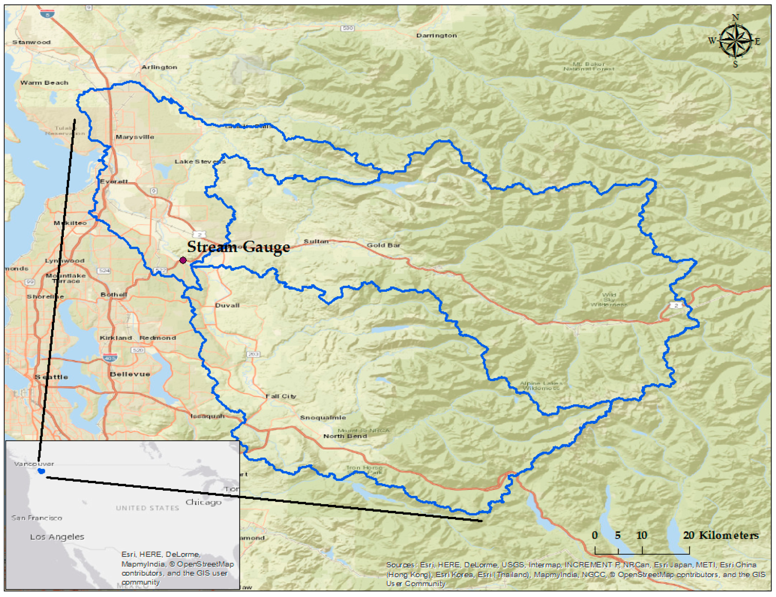
The framework is presented in the context of a case study based on the Snohomish River Basin located near Monroe, WA (Figure 2). This river basin is of particular interest for this case study because river peak flows are sensitive to rain, snow, and rain-on-snow events. The basin has frequent fluvial flooding, with overtopping expected to happen every 2 to 5 years [50]. The Snohomish River Basin belongs to the U.S. Pacific Northwest region, which was projected to experience the temporal and spatial changes in precipitation, with possible shifts of high (for example, flood) and low flow extremes [51].
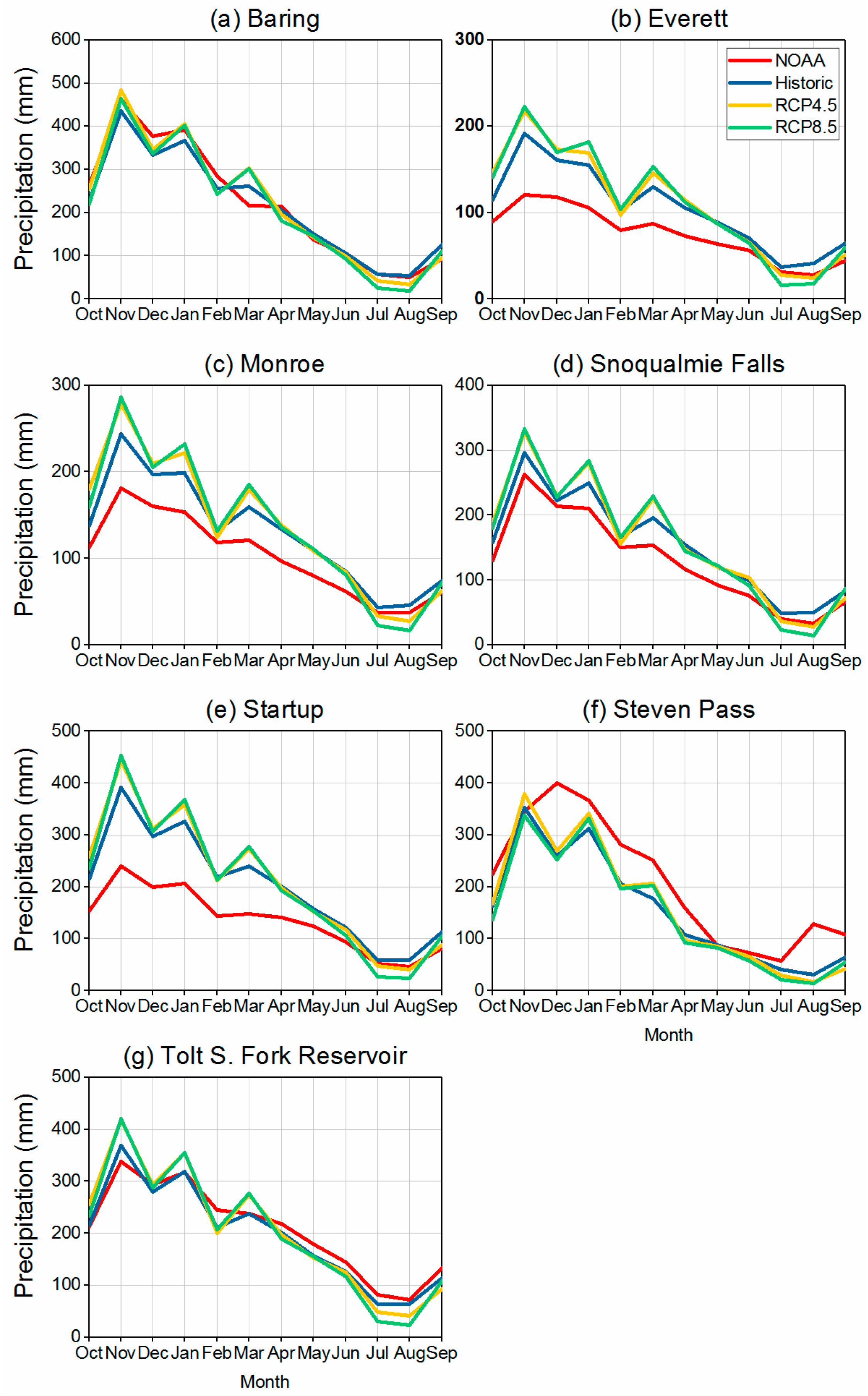
Downscaled precipitation from the previously described RCM was compared to the U.S. National Oceanic and Atmospheric Administration (NOAA)’s Global Historical Climatology Network-Daily (GHCN-D) database which provides the observed precipitation records. Seven sites were selected for having the sufficient length of record and representative locations and elevations within the watershed (Table 1).
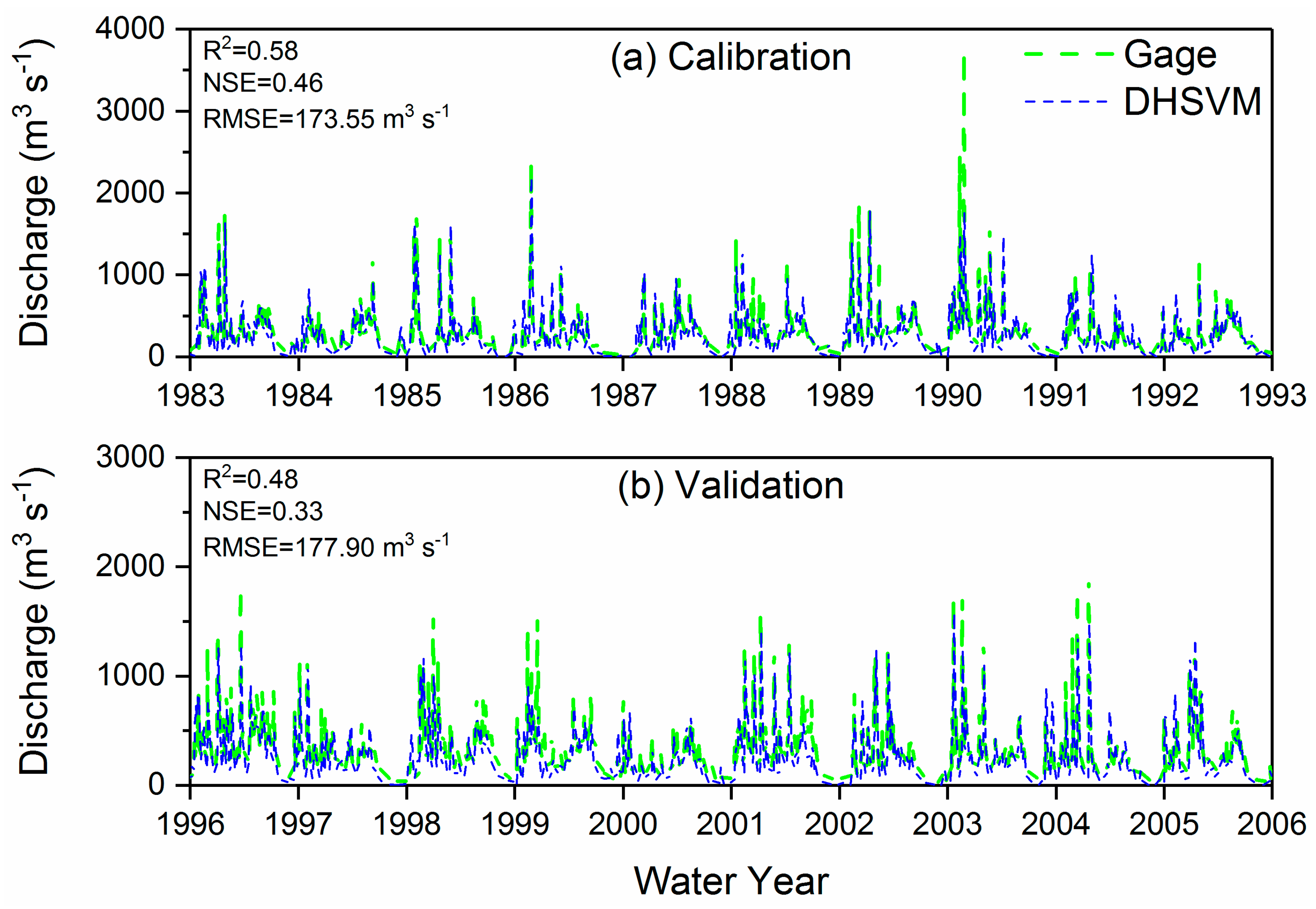
The DHSVM model was established for the Snohomish basin at a 150-m resolution using the previously described meteorological forcing data [29]. The DHSVM calibration and validation period, each a 10-year period, was driven by meteorological observations available in the NLDAS-2 dataset (Figure 3). The calibration and validation point was at a USGS stream gage location (ID: 12150800 Snohomish River near Monroe, WA, USA) near the downstream end of the basin. As noted previously, the DHSVM model was calibrated with a specific focus on maximizing the fit relative to extreme events and not low and medium flow events. As a result, the overall measures of fit are lower than what is normally anticipated. The calibrated and validated DHSVM model was rerun using the RCM historic, RCP4.5, and RCP8.5 meteorological forcings under the time periods shown in Table 2.
Using the DHSVM simulation output for the historic and future time periods in the Snohomish River Basin, statistical distributions of river discharge on the Snohomish River were developed and more than 140 samples from each statistical distribution were selected to drive high-resolution (30 m) hydrodynamic simulations.
As mentioned previously, a definition of the spatial aggregation unit and associated monetary value is needed to assess the damage. In this case study, the 2011 Snohomish County-assessed parcel dataset was used to provide the asset value (structural value) for consequence analysis. However, the parcel footprint was not used as the spatial aggregation unit. Rather, an approach was utilized to enhance the spatial resolution of structural representation and avoid estimation of damage in large parcels where the structural footprint is small. To accomplish this, the imperviousness percentages (30 m) from the 2011 U.S. National Land Cover Database was used to filter out the non-developed areas within a parcel. The structural asset value of a given parcel was distributed as a function of imperviousness across the grid cells within the parcel, such that the distributed structural value is conserved when compared to the total parcel value.
4. Results and Discussion
4.1. Precipitation Analysis
Mean-monthly comparisons of precipitation were made to understand the potential cascading bias in the development of local-scale, actionable information. Precipitation from each climate scenario was aggregated to mean-monthly values and compared to the seven weather stations. The precipitation of the historic scenario appears to over-predict at stations lower than 100 m, while it generally matched well with the observations at higher elevations (Figure 4). While not fully understood, plausible explanations for this variability is that the areas of lower elevation are subject to local disturbances (for example, urban impacts, local-scale orographic effects), which are not likely well represented by the RCM. Most importantly, it is not believed that these inconsistencies at lower elevations will have an impact on the outcomes of this study since the majority of the river flow generated originates in the upper elevations. The precipitation curves from both RCP scenarios are consistently higher when compared to historic precipitation, indicating an increasing trend in the precipitation amount projected for the study area. Notably, both RCP scenarios show increased winter precipitation and decreased summer precipitation relative to the historic scenario, a potentially important shift when considering the potential downstream impacts for changes in rain, snow, and rain-on-snow events and the preparation for such events.
4.2. Streamflow Simulation
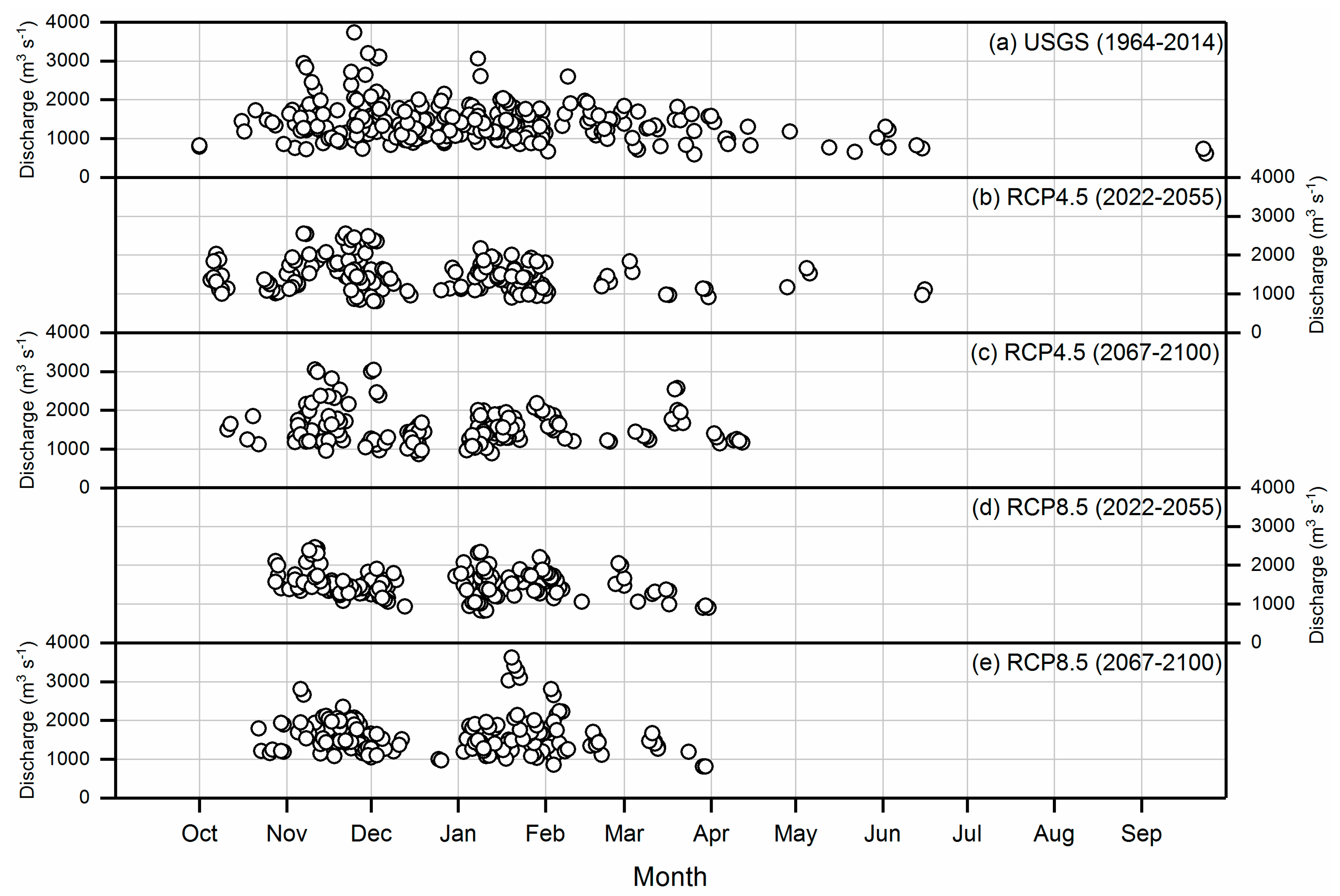
The calibrated and validated DHSVM model was used to predict river flow for both climate scenarios and were subsequently compared to the gauged stream flows representing the current condition. To closely examine the potential impact of the temporal shift in precipitation on the timing of annual peak discharge, five occurrences of maximum daily flow were selected for each year in the future period and compared to the gauge observations. For both the RCP4.5 and the RCP8.5 scenarios, there is a clear decrease in the number of months in which the peak flows are simulated to occur (Figure 5). That is, there are fewer occurrences of peak flow during the spring and summer months and an increase in the occurrence of peak flows during the winter months. This finding is consistent with the previous observation in this study where projected precipitation extremes tended to shift from the spring and summer months to winter months. Comparing the two future scenarios, the RCP8.5 scenario tends to have a stronger shift to winter peaks, a potentially important distinction as we compare the potential flood risk relative to carbon scenarios.
4.3. Streamflow Frequency Analysis
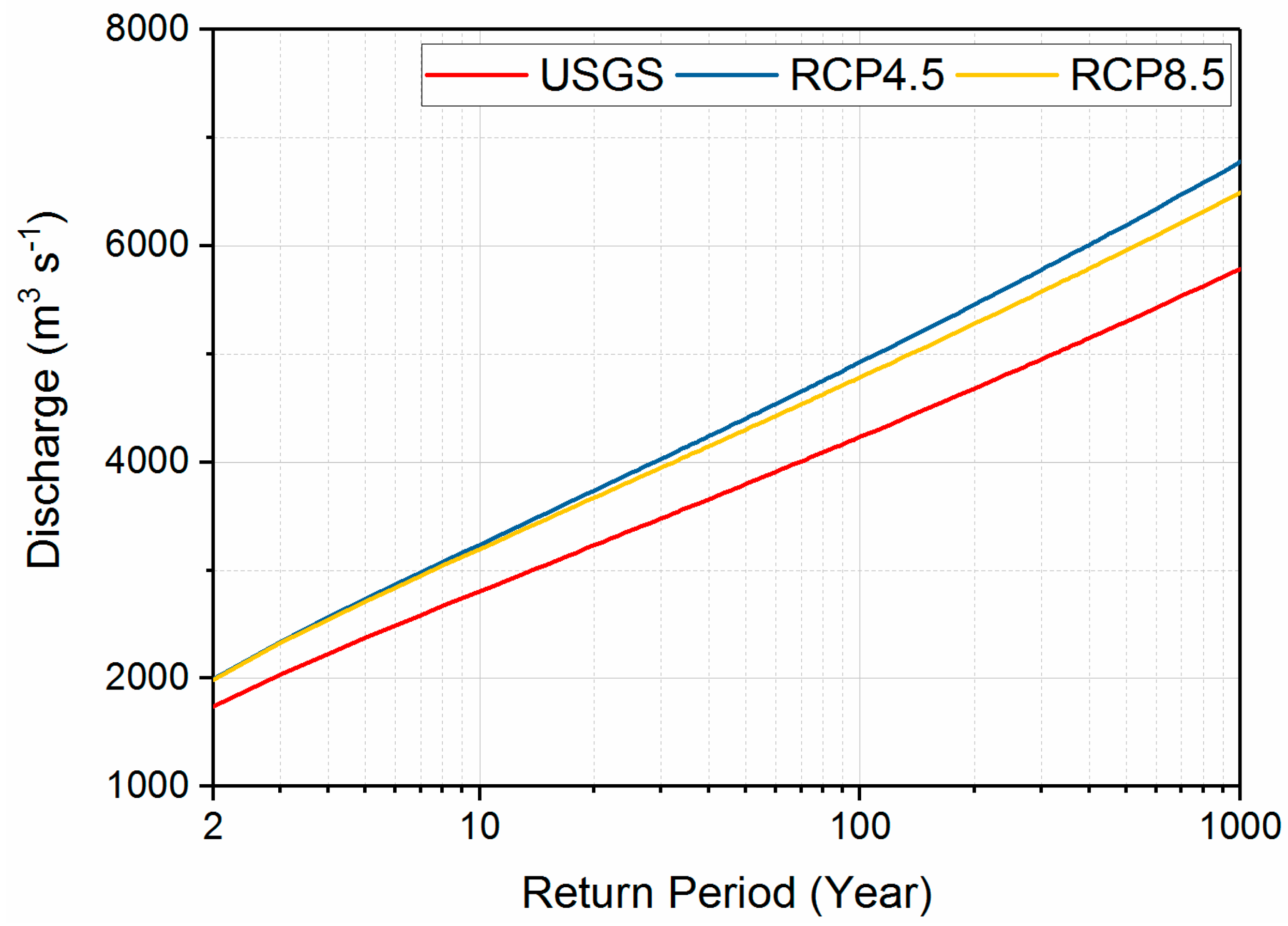
Traditional frequency analyses and those prescribed in flood insurance studies, such as the Bulletin 17C method, implicitly assume a stationary distribution. We utilized the Bulletin 17C method first to generate the frequency distribution of the combined periods (2022–2100) (Figure 6). However, to better address potential non-stationarities, we employ an approach where each carbon scenario was divided into two time windows which we considered to be stationary. To evaluate the validity of this assumption, we tested for non-stationarity using the Mann-Kendall test [17,34,52,53]. The test for non-stationarity included the entire time series of annual extremes in addition to a test for non-stationarity in the shorter time windows. For p-values less than 0.05, we reject the null hypothesis and determine that the time series is non-stationary. Otherwise, the data is determined to be stationary. The result of the Mann-Kendall test is summarized in Table 3 and indicate that the complete time series of annual extremes is non-stationary. However, the test shows that the majority of the smaller time windows can be considered stationary with the exception of the latter time period of RCP4.5, which exhibited a downward trend in annual extreme flows.
While non-stationarities exist in streamflow data when considering the full time series of flows and there are statistical approaches to account for these, the traditional methods (Bulletin 17C) were used so as to show the possible outcomes using these approaches. The impact of the long-term trend can effectively be evaluated by comparison of the separate, shorter time windows that are considered stationary.
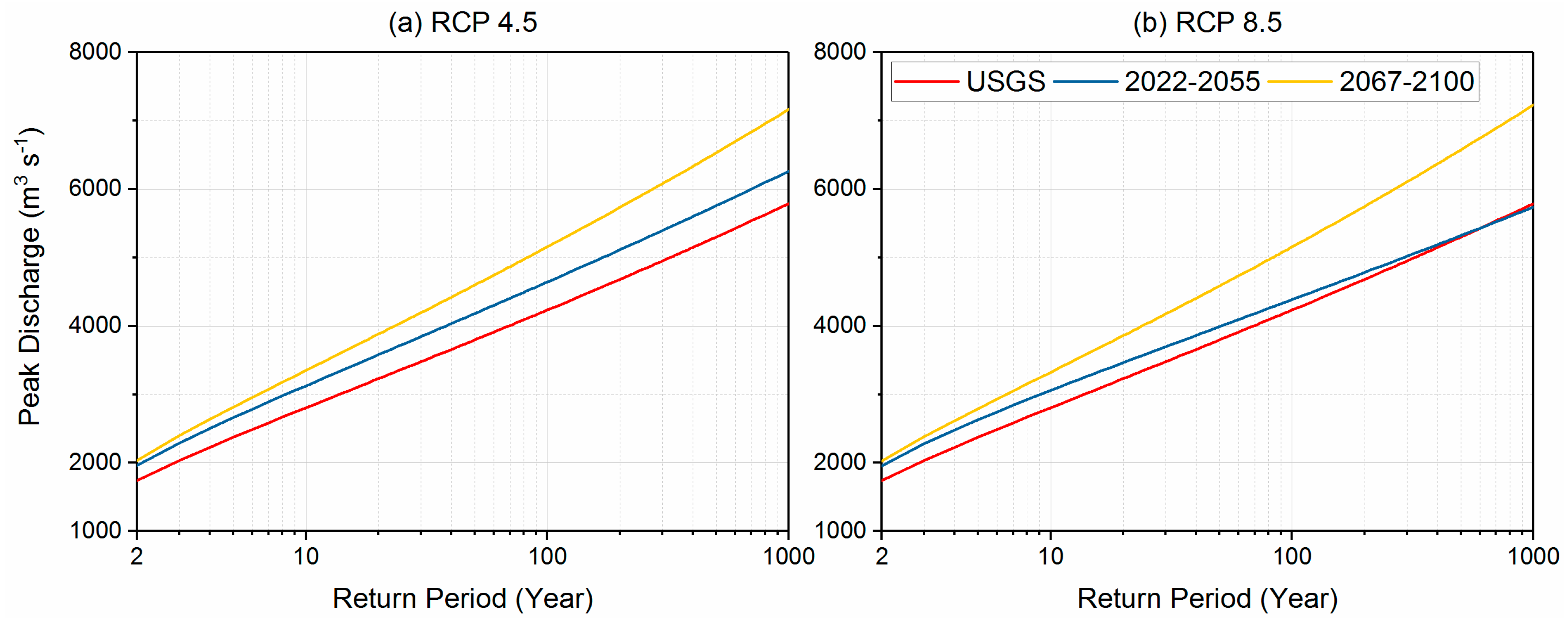
Using the frequency distributions developed using the Bulletin 17C method, the direct comparison of annual return period events can be made to quantify relative change in intensity and frequency of extreme flood events. A comparison of the two windows (2022–2055 and 2067–2100), therefore, could indirectly exhibit the non-stationarity of climate changes over longer time scales (not within the 30-year period) (Figure 7). A significant difference between the two future scenarios was found for the period 2022–2055. Compared to RCP4.5, RCP8.5 generally exhibits a smaller increase in peak flows and is especially pronounced for the more extreme return period events, consistent with previous findings [54]. Although the projected peak flows of our RCP8.5 scenario was slightly lower than the historic conditions for the largest return periods, this was also found by a previous study using 10 GCMs. Simulating rare events with large return periods using GCM meteorological data is a persistent challenge [54] (p. 181). Because the occurrence of precipitation peaks and runoff peaks are projected to be toward the winter months, this finding could be expected to be related to the timing of rain-on-snow events.
The latter future period (2067–2100) for both scenarios all show an increase in the peak river flow when compared to the early future period (2022–2055) (Figure 7). This exposes a non-stationary condition in the magnitude of peak discharges for a given flood probability, and conversely, a non-stationary reduction in the return interval for the given peak discharge. These non-stationary changes could be expected to be more intense for the rarer but more severe floods and, therefore, be associated with more significant consequences.
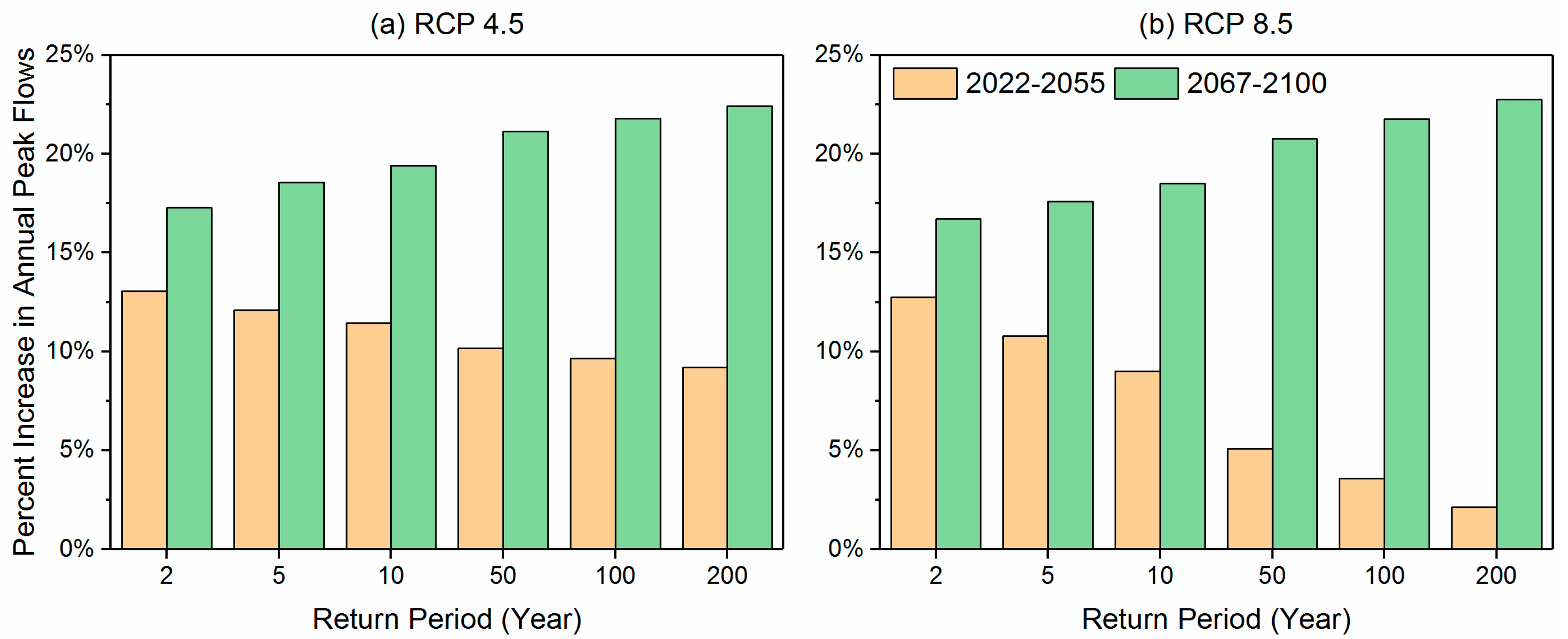
An example can be given to take a closer look at these non-stationary changes. The low end of the return periods is more closely aligned since they were established on a fair amount of historical events (and, therefore, more certainty) than the larger return periods which are established based on few, rare events (Figure 7). Among the selected six return periods shown in Figure 8, both climate scenarios projected a larger magnitude of peak flows compared to the historic period. That is, the new 10-year return period in RCP4.5 and RCP8.5 could have a more than 9% increase in the peak flows when compared historically. Conversely, the historic 10-year peak flow would be expected to happen, on average, every 5–7 years under both climate scenarios. Even within the selected 200-year return period time window, the non-stationarity was clearly exhibited with a reverse trend between the two periods. That is, the percent change in the peak discharges for both RCP4.5 and RCP8.5 scenarios were projected to decrease (overall a net increase) with the increasing return period during 2022–2055, while the percent change in the peak discharges for both scenarios increased with increasing return period during 2067–2100.
Given the general perception of increased impacts for more extreme climate scenarios, it may be non-intuitive to expect a reduced potential for flooding under warmer climate conditions as we see with the statistical distribution in this case study that has been post-bias corrected. Peak flows in a river system have a complex, nonlinear relationship with precipitation dynamics and other factors, including catchment size and topographic effects. This finding is not inconsistent with other findings in the literature where some studies have found a decrease in the peak flow magnitude with more extreme climate scenarios [55]. The purpose of this study is to demonstrate the ability to connect multiple models at multiple scales and resolutions, not necessarily to uncover the relationship between snow and rain dynamics on peak runoff. A worthy follow-on study should focus on uncovering this relationship by investigating the mechanisms governing runoff in this specific location (considering local effects such as topography) as influenced by the climate scenarios.
4.4. Quantification of Consequences
The end products of the integrated multi-scale, multi-model framework quantify the flood risk at a local scale. In this case for demonstration of the framework, only the latter time period (2067–2100) of RCP4.5 is considered when evaluating future flood risk since RCP4.5 is a middle-of-the-road representation for climate in the future.
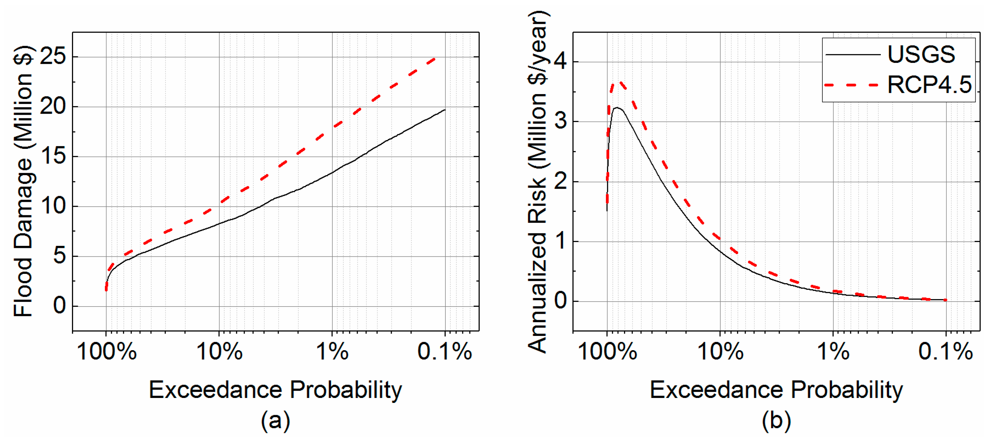
To capture a likely chance for change under future climate scenarios, only the USGS (used as a baseline) and RCP4.5 frequency distributions were used. Due to the projected climate change (from USGS to RCP4.5), the studied watershed would experience 24%, 33%, and 29% increases in both direct damage and annualized risk (with the same rates) for the 10-year, 100-year, and 1000-year floods (Figure 9). The maximum annualized flood risk was raised by 15% in the RCP4.5 scenario, while the peak of each annualized flood risk is at 1.2-years. The low return period with maximum annualized risk indicates that mitigation measures should target the repetitive, lower magnitude floods for this region. The damage caused by the current 10-year flood would be expected to be equivalent to damage of the future 5-year flood, while the damage caused by the current 100-year flood would be projected to be similar to the future 29-year flood. This further validates the need to include climate scenarios with a local-scale, actionable information when developing mitigation and adaptation plans in flood risk.
5. Conclusions
Floods are a persistent threat that is expected to increase in occurrence and damage as we move into an uncertain climate future. Methods are required to translate global-scale climate projections into actionable information. The objective of this study was to demonstrate an application of a multi-model, multi-scale approach whereby climate model output can be used to develop actionable information in flood risk management projects, a direct need relative to recent changes in flood risk management standards. To accomplish this, an RCM (1/8 degree), a distributed hydrologic model (150 m), and a hydrodynamic model (30 m) were integrated to develop flood risk estimates under current and future climate scenarios. The integrated approach applied to the Snohomish River Basin revealed several findings, including the following:
- (1)
- Precipitation and annual peak streamflow is projected to shift from the late spring and summer months to earlier in the winter season;
- (2)
- There is an observed non-stationarity of annual peak discharges as we move into future scenarios, both under the RCP 4.5 and RCP 8.5 scenarios. The magnitude of river discharge annual exceedance was shown to increase by as much as 22% and the annualized flood risk increasing by as much as 33% in the most extreme cases in future climate scenarios.
- (3)
- There are non-linearities associated with the hydrological response under climate scenarios. For example, in this river basin, the RCP 4.5 scenario projected overall higher peak flows compared to the RCP 8.5 scenario despite slight increases in the mean-monthly precipitation under RCP 8.5. This highlights a need to further understand the mechanics associated with runoff where there are potential impacts from changes in rain, snow, and rain-on-snow events.
This work successfully establishes an integrated framework to develop local-scale flood risk information. While this research did not rigorously address uncertainty in climate prediction, such an integrated approach provides opportunities to enable robust uncertainty quantification in flood risk management. For example, an uncertainty that could be further explored is the relative under-prediction of extreme precipitation events in GCMS and how this translates to decisions in flood risk management. This is not a new problem as previous studies have found that similar integrated modeling approaches have been limited by the under-performance of rainfall predictions [21,56,57]. The integrated approach provides an opportunity to easily incorporate multiple GCM/RCM models into the multi-scale, multi-model approach such that the ensembles of the simulations from a global to local scale can be completed and uncertainties associated with climate projections can be robustly evaluated.
Finally, this integrated approach has been shown to have application in flood risk management by looking at potential changes in damage associated with non-stationarity in flood frequency. The integrated approach can also be used to develop local-scale water management decisions relative to temporal shifts in annual runoff volume under water-stressed conditions.
Author Contributions
D.R.J. conceived and designed the project; D.R.J. and C.L.R. performed the model; S.R.W., D.R.J., Y.F., and C.L.R. analyzed the data; D.R.J., Y.F., and C.L.R. wrote the paper.
Acknowledgments
This work was mainly sponsored by Pacific Northwest National Laboratory (PNNL) Laboratory Directed Research and Development program. PNNL is operated for U.S. Department of Energy by Battelle Memorial Institute under contract DE-AC05-76RL01830. The work also received kind supports from the Snohomish County, WA, U.S.
Conflicts of Interest
The authors declare no conflict of interest.
References
- Fowler, H.J.; Wilby, R.L. Detecting changes in seasonal precipitation extremes using regional climate model projections: Implications for managing fluvial flood risk. Water Resour. Res. 2010, 46, W03525. [Google Scholar] [CrossRef]
- Falter, D.; Schröter, K.; Dung, N.V.; Vorogushyn, S.; Kreibich, H.; Hundecha, Y.; Apel, H.; Merz, B. Spatially coherent flood risk assessment based on long-term continuous simulation with a coupled model chain. J. Hydrol. 2015, 524, 182–193. [Google Scholar] [CrossRef] [Green Version]
- Cheng, L.; AghaKouchak, A. Nonstationary precipitation intensity-duration-frequency curves for infrastructure design in a changing climate. Sci. Rep. 2014, 4, 7093. [Google Scholar] [CrossRef] [PubMed]
- Mailhot, A.; Duchesne, S. Design Criteria of Urban Drainage Infrastructures under Climate Change. J. Water Resour. Plan. Manag. 2010, 136, 201–208. [Google Scholar] [CrossRef]
- Kim, B.S.; Kim, B.K.; Kwon, H.H. Assessment of the impact of climate change on the flow regime of the Han River basin using indicators of hydrologic alteration. Hydrol. Process. 2011, 25, 691–704. [Google Scholar] [CrossRef]
- Wood, A.W.; Leung, L.R.; Sridhar, V.; Lettenmaier, D.P. Hydrologic Implications of Dynamical and Statistical Approaches to Downscaling Climate Model Outputs. Clim. Chang. 2004, 62, 189–216. [Google Scholar] [CrossRef]
- Prudhomme, C.; Jakob, D.; Svensson, C. Uncertainty and climate change impact on the flood regime of small UK catchments. J. Hydrol. 2003, 277, 1–23. [Google Scholar] [CrossRef]
- Dulie, V.; Zhang, Y.; Salathe, E.P. Extreme precipitation and temperature over the U.S. Pacific Northwest: A comparison between observations, reanalysis data, and regional models. J. Clim. 2011, 24, 1950–1964. [Google Scholar] [CrossRef]
- Fowler, H.J.; Blenkinsop, S.; Tebaldi, C. Linking climate change modelling to impacts studies: Recent advances in downscaling techniques for hydrological modelling. Int. J. Climatol. 2007, 27, 1547–1578. [Google Scholar] [CrossRef]
- Xu, C.-Y. From GCMs to river flow: A review of downscaling methods and hydrologic modelling approaches. Prog. Phys. Geogr. 1999, 23, 229–249. [Google Scholar] [CrossRef]
- Prudhomme, C.; Reynard, N.; Crooks, S. Downscaling of global climate models for flood frequency analysis: Where are we now? Hydrol. Process. 2002, 16, 1137–1150. [Google Scholar] [CrossRef]
- Sunyer, M.A.; Hundecha, Y.; Lawrence, D.; Madsen, H.; Willems, P.; Martinkova, M.; Vormoor, K.; Bürger, G.; Hanel, M.; Kriaučiuniene, J.; et al. Inter-comparison of statistical downscaling methods for projection of extreme precipitation in Europe. Hydrol. Earth Syst. Sci. 2015, 19, 1827–1847. [Google Scholar] [CrossRef] [Green Version]
- Burton, A.; Fowler, H.J.; Blenkinsop, S.; Kilsby, C.G. Downscaling transient climate change using a Neyman-Scott Rectangular Pulses stochastic rainfall model. J. Hydrol. 2010, 381, 18–32. [Google Scholar] [CrossRef]
- Vormoor, K.; Lawrence, D.; Heistermann, M.; Bronstert, A. Climate change impacts on the seasonality and generation processes of floods—Projections and uncertainties for catchments with mixed snowmelt/rainfall regimes. Hydrol. Earth Syst. Sci. 2015, 19, 913–931. [Google Scholar] [CrossRef]
- Mizukami, N.; Clark, M.P.; Gutmann, E.D.; Mendoza, P.A.; Newman, A.J.; Nijssen, B.; Livneh, B.; Hay, L.E.; Arnold, J.R.; Brekke, L.D. Implications of the Methodological Choices for Hydrologic Portrayals of Climate Change over the Contiguous United States: Statistically Downscaled Forcing Data and Hydrologic Models. J. Hydrometeorol. 2016, 17, 73–98. [Google Scholar] [CrossRef]
- Camici, S.; Brocca, L.; Moramarco, T. Accuracy versus variability of climate projections for flood assessment in central Italy. Clim. Chang. 2017, 141, 273–286. [Google Scholar] [CrossRef]
- Khaliq, M.N.; Ouarda, T.B.M.J.; Ondo, J.C.; Gachon, P.; Bobée, B. Frequency analysis of a sequence of dependent and/or non-stationary hydro-meteorological observations: A review. J. Hydrol. 2006, 329, 534–552. [Google Scholar] [CrossRef]
- Teng, J.; Jakeman, A.J.; Vaze, J.; Croke, B.F.W.; Dutta, D.; Kim, S. Flood inundation modelling: A review of methods, recent advances and uncertainty analysis. Environ. Model. Softw. 2017, 90, 201–216. [Google Scholar] [CrossRef]
- Kalyanapu, A.; Judi, D.; McPherson, T.; Burian, S. Monte Carlo-based flood modelling framework for estimating probability weighted flood risk. J. Flood Risk Manag. 2012, 5, 37–48. [Google Scholar] [CrossRef]
- Falter, D.; Dung, N.; Vorogushyn, S.; Schröter, K.; Hundecha, Y.; Kreibich, H.; Apel, H.; Theisselmann, F.; Merz, B. Continuous, large-scale simulation model for flood risk assessments: Proof-of-concept. J. Flood Risk Manag. 2016, 9, 3–21. [Google Scholar] [CrossRef]
- Alfieri, L.; Dottori, F.; Betts, R.; Salamon, P.; Feyen, L. Multi-model projections of river flood risk in Europe under global warming. Climate 2018, 6, 6. [Google Scholar] [CrossRef]
- Kraucunas, I.; Clarke, L.; Dirks, J.; Hathaway, J.; Hejazi, M.; Hibbard, K.; Huang, M.; Jin, C.; Kintner-Meyer, M.; van Dam, K.K. Investigating the nexus of climate, energy, water, and land at decision-relevant scales: The Platform for Regional Integrated Modeling and Analysis (PRIMA). Clim. Chang. 2015, 129, 573–588. [Google Scholar] [CrossRef]
- Gao, Y.; Leung, L.R.; Lu, J.; Liu, Y.; Huang, M.; Qian, Y. Robust spring drying in the southwestern US and seasonal migration of wet/dry patterns in a warmer climate. Geophys. Res. Lett. 2014, 41, 1745–1751. [Google Scholar] [CrossRef]
- Skamarock, W.C.; Klemp, J.B.; Dudhia, J.; Gill, D.O.; Barker, D.M.; Duda, M.G.; Huang, X.-Y.; Wang, W.; Powers, J.G. A Description of the Advanced Research WRF Version 3; NCAR Technical Note; National Center for Atmospheric Research: Boulder, CO, USA, 2008. [Google Scholar]
- Xia, Y.; Mitchell, K.; Ek, M.; Sheffield, J.; Cosgrove, B.; Wood, E.; Luo, L.; Alonge, C.; Wei, H.; Meng, J.; et al. Continental-scale water and energy flux analysis and validation for the North American Land Data Assimilation System project phase 2 (NLDAS-2): 1. Intercomparison and application of model products. J. Geophys. Res. Atmos. 2012, 117, D03109. [Google Scholar] [CrossRef]
- Hejazi, M.I.; Voisin, N.; Liu, L.; Bramer, L.M.; Fortin, D.C.; Hathaway, J.E.; Huang, M.; Kyle, P.; Leung, L.R.; Li, H.-Y. 21st century United States emissions mitigation could increase water stress more than the climate change it is mitigating. Proc. Natl. Acad. Sci. USA 2015, 112, 10635–10640. [Google Scholar] [CrossRef] [PubMed]
- Van Vuuren, D.P.; Edmonds, J.; Kainuma, M.; Riahi, K.; Thomson, A.; Hibbard, K.; Hurtt, G.C.; Kram, T.; Krey, V.; Lamarque, J.-F.; et al. The representative concentration pathways: An overview. Clim. Chang. 2011, 109, 5–31. [Google Scholar] [CrossRef]
- Wigmosta, M.S.; Vail, L.W.; Lettenmaier, D.P. A distributed hydrology-vegetation model for complex terrain. Water Resour. Res. 1994, 30, 1665–1679. [Google Scholar] [CrossRef]
- Yang, Z.; Wang, T.; Voisin, N.; Copping, A. Estuarine response to river flow and sea-level rise under future climate change and human development. Estuar. Coast. Shelf Sci. 2015, 156, 19–30. [Google Scholar] [CrossRef]
- Maidment, D.R. Handbook of Hydrology; McGraw-Hill: New York, NY, USA, 1993; Volume 1. [Google Scholar]
- Yapo, P.O.; Gupta, H.V.; Sorooshian, S. Multi-objective global optimization for hydrologic models. J. Hydrol. 1998, 204, 83–97. [Google Scholar] [CrossRef]
- Moriasi, D.N.; Arnold, J.G.; Van Liew, M.W.; Bingner, R.L.; Harmel, R.D.; Veith, T.L. Model evaluation guidelines for systematic quantification of accuracy in watershed simulations. Trans. ASABE 2007, 50, 885–900. [Google Scholar] [CrossRef]
- England, J.F., Jr.; Cohn, T.A.; Faber, B.A.; Stedinger, J.R.; Thomas, W.O., Jr.; Veilleux, A.G.; Kiang, J.E.; Mason, R.R., Jr. Guidelines for Determining Flood Flow Frequency—Bulletin 17C; US Geological Survey: Reston, VA, USA, 2018.
- Cunderlik, J.M.; Burn, D.H. Non-stationary pooled flood frequency analysis. J. Hydrol. 2003, 276, 210–223. [Google Scholar] [CrossRef]
- Brigode, P.; Bernardara, P.; Paquet, E.; Gailhard, J.; Garavaglia, F.; Merz, R.; Mićović, Z.; Lawrence, D.; Ribstein, P. Sensitivity analysis of SCHADEX extreme flood estimations to observed hydrometeorological variability. Water Resour. Res. 2014, 50, 353–370. [Google Scholar] [CrossRef] [Green Version]
- Qi, W.; Zhang, C.; Fu, G.; Zhou, H.; Liu, J. Quantifying Uncertainties in Extreme Flood Predictions under Climate Change for a Medium-Sized Basin in Northeastern China. J. Hydrometeorol. 2016, 17, 3099–3112. [Google Scholar] [CrossRef]
- Hundecha, Y.; Sunyer, M.A.; Lawrence, D.; Madsen, H.; Willems, P.; Bürger, G.; Kriaučiūnienė, J.; Loukas, A.; Martinkova, M.; Osuch, M.; et al. Inter-comparison of statistical downscaling methods for projection of extreme flow indices across Europe. J. Hydrol. 2016, 541, 1273–1286. [Google Scholar] [CrossRef]
- Jiang, P.; Gautam, M.R.; Zhu, J.; Yu, Z. How well do the GCMs/RCMs capture the multi-scale temporal variability of precipitation in the Southwestern United States? J. Hydrol. 2013, 479, 75–85. [Google Scholar] [CrossRef]
- Camici, S.; Brocca, L.; Melone, F.; Moramarco, T. Impact of climate change on flood frequency using different climate models and downscaling approaches. J. Hydrol. Eng. 2014, 19, 04014002. [Google Scholar] [CrossRef]
- Condon, L.E.; Gangopadhyay, S.; Pruitt, T. Climate change and non-stationary flood risk for the upper Truckee River basin. Hydrol. Earth Syst. Sci. 2015, 19, 159–175. [Google Scholar] [CrossRef] [Green Version]
- Seidou, O.; Ramsay, A.; Nistor, I. Climate change impacts on extreme floods I: Combining imperfect deterministic simulations and non-stationary frequency analysis. Nat. Hazards 2012, 61, 647–659. [Google Scholar] [CrossRef]
- Kourgialas, N.N.; Dokou, Z.; Karatzas, G.P. Statistical analysis and ANN modeling for predicting hydrological extremes under climate change scenarios: The example of a small Mediterranean agro-watershed. J. Environ. Manag. 2015, 154, 86–101. [Google Scholar] [CrossRef] [PubMed]
- Jaw, T.; Li, J.; Hsu, K.L.; Sorooshian, S.; Driouech, F. Evaluation for Moroccan dynamically downscaled precipitation from GCM CHAM5 and its regional hydrologic response. J. Hydrol. Reg. Stud. 2015, 3, 359–378. [Google Scholar] [CrossRef]
- Lu, Y.; Qin, X.S.; Xie, Y.J. An integrated statistical and data-driven framework for supporting flood risk analysis under climate change. J. Hydrol. 2016, 533, 28–39. [Google Scholar] [CrossRef]
- Miller, W.P.; Butler, R.A.; Piechota, T.; Prairie, J.; Grantz, K.; DeRosa, G. Water management decisions using multiple hydrologic models within the San Juan River basin under changing climate conditions. J. Water Resour. Plan. Manag. 2012, 138, 412–420. [Google Scholar] [CrossRef]
- Judi, D.R.; Burian, S.J.; McPherson, T.N. Two-dimensional fast-response flood modeling: Desktop parallel computing and domain tracking. J. Comput. Civ. Eng. 2010, 25, 184–191. [Google Scholar] [CrossRef]
- Scawthorn, C.; Flores, P.; Blais, N.; Seligson, H.; Tate, E.; Chang, S.; Mifflin, E.; Thomas, W.; Murphy, J.; Jones, C.; et al. HAZUS-MH Flood Loss Estimation Methodology. II. Damage and Loss Assessment. Nat. Hazards Rev. 2006, 7, 72–81. [Google Scholar] [CrossRef]
- FEMA. Technical Bulletin 10: Ensuring that Structures Built on Fill in or near Special Flood Hazard Areas Are Reasonably Safe from Flooding; FEMA: Washington, DC, USA, 2001.
- Kalyanapu, A.J.; Judi, D.R.; McPherson, T.N.; Burian, S.J. Annualised risk analysis approach to recommend appropriate level of flood control: Application to Swannanoa river watershed. J. Flood Risk Manag. 2015, 8, 368–385. [Google Scholar] [CrossRef]
- Snohomish County Emergency Management. Snohomish County Hazard Mitigation Plan: Summary; Snohomish County Emergency Management: Everett, WA, USA, 2015.
- Hamlet, A.F. Assessing water resources adaptive capacity to climate change impacts in the Pacific Northwest Region of North America. Hydrol. Earth Syst. Sci. 2011, 15, 1427–1443. [Google Scholar] [CrossRef] [Green Version]
- Leclerc, M.; Ouarda, T.B.M.J. Non-stationary regional flood frequency analysis at ungauged sites. J. Hydrol. 2007, 343, 254–265. [Google Scholar] [CrossRef]
- Cheng, L.; AghaKouchak, A.; Gilleland, E.; Katz, R.W. Non-stationary extreme value analysis in a changing climate. Clim. Chang. 2014, 127, 353–369. [Google Scholar] [CrossRef]
- Snohomish County Emergency Management. Snohomish County Hazard Mitigation Plan: Volume 1 Risk Assessment; Snohomish County Emergency Management: Everett, WA, USA, 2015.
- Madsen, H.; Lawrence, D.; Lang, M.; Martinkova, M.; Kjeldsen, T.R. Review of trend analysis and climate change projections of extreme precipitation and floods in Europe. J. Hydrol. 2014, 519, 3634–3650. [Google Scholar] [CrossRef] [Green Version]
- Pappenberger, F.; Beven, K.J.; Hunter, N.M.; Bates, P.D.; Gouweleeuw, B.T.; Thielen, J.; De Roo, A.P.J. Cascading model uncertainty from medium range weather forecasts (10 days) through a rainfall-runoff model to flood inundation predictions within the European Flood Forecasting System (EFFS). Hydrol. Earth Syst. Sci. Discuss. 2005, 9, 381–393. [Google Scholar] [CrossRef] [Green Version]
- Betts, R.A.; Alfieri, L.; Bradshaw, C.; Caesar, J.; Feyen, L.; Friedlingstein, P.; Gohar, L.; Koutroulis, A.; Lewis, K.; Morfopoulos, C.; et al. Changes in climate extremes, fresh water availability and vulnerability to food insecurity projected at 1.5 °C and 2 °C global warming with a higher-resolution global climate model. Philos. Trans. R. Soc. A Math. Phys. Eng. Sci. 2018, 376. [Google Scholar] [CrossRef] [PubMed]
Figure 1.
The integrated multi-scale, multi-model framework for flood risk estimation.

Figure 2.
The Snohomish watershed (blue lines) and the location of the USGS stream gauge near Monroe, WA, USA.
Figure 2.
The Snohomish watershed (blue lines) and the location of the USGS stream gauge near Monroe, WA, USA.

Figure 3.
The DHSVM calibration and validation at Monroe, WA, USA.

Figure 4.
The mean monthly precipitation from seven climate data sets at seven Snohomish watershed locations.
Figure 4.
The mean monthly precipitation from seven climate data sets at seven Snohomish watershed locations.

Figure 5.
The timing of the five largest daily flows in each water year for different scenarios.

Figure 6.
The frequency distribution of annual peak flow with two combined periods (RCP4.5 and RCP8.5 period 1 and 2) and for USGS instantaneous observations using the Bulletin 17C method.
Figure 6.
The frequency distribution of annual peak flow with two combined periods (RCP4.5 and RCP8.5 period 1 and 2) and for USGS instantaneous observations using the Bulletin 17C method.

Figure 7.
The frequency curves of the annual peak flow at Monroe for USGS instantaneous observations (1964–2014), RCP4.5 (a); and RCP8.5 (b) made by the Bulletin 17C method.
Figure 7.
The frequency curves of the annual peak flow at Monroe for USGS instantaneous observations (1964–2014), RCP4.5 (a); and RCP8.5 (b) made by the Bulletin 17C method.

Figure 8.
The percentage increase of estimated future peak flows for bias-corrected RCP4.5 (a) and RCP8.5 (b) over the historic USGS instantaneous peak flows.
Figure 8.
The percentage increase of estimated future peak flows for bias-corrected RCP4.5 (a) and RCP8.5 (b) over the historic USGS instantaneous peak flows.

Figure 9.
The damage (a) and annualized risk (b) of USGS and RCP4.5 flow conditions.


Table 1.
The NOAA Daily Precipitation Sites. Only calendar years with at least 300 recorded days were included in the analysis.
Table 1.
The NOAA Daily Precipitation Sites. Only calendar years with at least 300 recorded days were included in the analysis.
| Station | Elevation | Water Years | Total of Years |
|---|---|---|---|
| Baring (47.7722° N, 121.4819° W) | 235 m | 1978–1998, 2000, 2002–2003 | 24 |
| Everett (47.9753° N, 122.1950° W) | 18 m | 1978–2003 | 26 |
| Monroe (47.8453° N, 121.9944° W) | 37 m | 1978–2003 | 26 |
| Snoqualmie Falls (47.5414° N, 121.8361° W) | 134 m | 1978–1995, 1997–2003 | 25 |
| Startup (47.8664° N, 121.7175° W) | 52 m | 1978–2003 | 26 |
| Stevens Pass (47.7372° N, 121.0914° W) | 1241 m | 1978–1980, 1995–1997, 1999, 2000 | 8 |
| Tolt S. Fork Reservoir (47.7000° N, 121.6908° W) | 610 m | 1978–1984, 1986–1988, 1990–1991, 1993, 1995–2000, 2002–2003 | 21 |
Table 2.
The water years used for flow frequency analysis.
| Scenarios | Years |
|---|---|
| USGS | 1964–2014 |
| Historic | 1978–2003 |
| RCP4.5 | 2022–2055 (T1), 2067–2100 (T2) |
| RCP8.5 | 2022–2055 (T1), 2067–2100 (T1) |
Table 3.
The results of the Mann-Kendall test for data non-stationarity on annual extreme flows.
| Time Period | p-Value for Upward Trend | p-Value for Downward Trend | Stationarity Outcome |
|---|---|---|---|
| Historic | 0.08 | 0.92 | Stationary |
| RCP45_T1 | 0.19 | 0.81 | Stationary |
| RCP45_T2 | 0.98 | 0.02 | Non-Stationary |
| RCP85_T1 | 0.46 | 0.54 | Stationary |
| RCP85_T2 | 0.59 | 0.41 | Stationary |
| RCP45_T1 + T2 | 0.49 | 0.51 | Stationary |
| RCP85_T1 + T2 | 0.35 | 0.65 | Stationary |
| Historic + RCP45_T1 + T2 | 0.01 | 0.99 | Non-Stationary |
| Historic + RCP85_T1 + T2 | 0.00 | 1.00 | Non-Stationary |
© 2018 by the authors. Licensee MDPI, Basel, Switzerland. This article is an open access article distributed under the terms and conditions of the Creative Commons Attribution (CC BY) license (http://creativecommons.org/licenses/by/4.0/).
Share and Cite
MDPI and ACS Style
Judi, D.R.; Rakowski, C.L.; Waichler, S.R.; Feng, Y.; Wigmosta, M.S. Integrated Modeling Approach for the Development of Climate-Informed, Actionable Information. Water 2018, 10, 775. https://doi.org/10.3390/w10060775
AMA Style
Judi DR, Rakowski CL, Waichler SR, Feng Y, Wigmosta MS. Integrated Modeling Approach for the Development of Climate-Informed, Actionable Information. Water. 2018; 10(6):775. https://doi.org/10.3390/w10060775
Chicago/Turabian StyleJudi, David R., Cynthia L. Rakowski, Scott R. Waichler, Youcan Feng, and Mark S. Wigmosta. 2018. "Integrated Modeling Approach for the Development of Climate-Informed, Actionable Information" Water 10, no. 6: 775. https://doi.org/10.3390/w10060775
Note that from the first issue of 2016, this journal uses article numbers instead of page numbers. See further details here.