Development and Application of Advanced Muskingum Flood Routing Model Considering Continuous Flow


1
Research Center for Disaster Prevention Science and Technology, Korea University, Seoul 02841, Korea
2
School of Civil, Environmental and Architectural Engineering, Korea University, Seoul 02841, Korea
*
Author to whom correspondence should be addressed.
Water 2018, 10(6), 760; https://doi.org/10.3390/w10060760
Submission received: 21 May 2018
/
Revised: 8 June 2018
/
Accepted: 9 June 2018
/
Published: 11 June 2018
(This article belongs to the Section Hydrology)
Abstract
:The Muskingum flood routing model is a representative flood routing model. The field applicability of the Muskingum flood routing model is known to be good, and the structure of input data is simple. However, accurate flood routing cannot be conducted using current Muskingum flooding routing models due to the structural limitation of equations. The advanced nonlinear Muskingum flood routing model is suggested for improving accuracy, considering continuous flow using weighted inflow. Continuous flow means the past continuous inflows, including first and secondary inflow over time. Five flood data were selected for a comparison between the results of this study and previous ones. The sum of squares, root mean square errors, and Nash-Sutcliffe efficiency are applied in order to calculate the error values. The vision correction algorithm was used to estimate parameters in the new model. Generally, the new method yields better results than those described in previous studies, though it shows similar results with the most recent methods (NLMM-L) in some flood data. Finally, the new method and NLMM-L are applied for the prediction of Daechung flood data in Korea. The new method is useful in the prediction of outflows, because it shows better results than NLMM-L.
1. Introduction
The fundamental purpose of flooding routing is the estimation of the discharge flowing at river sites of interest. The results of flood routing models can be used for the design of various hydraulic structures in streams and rivers. Dams, levees, and flood barriers have been constructed in order to prevent flood disasters. Flood routing methods can be classified into hydraulic flood routing and hydrologic flood routing. Hydraulic flood routing is based on computation considering boundary conditions, including the initial condition using the continuity and momentum equations, which govern equations of unsteady, non-uniform flow in upstream and downstream directions. It can exhibit high accuracy, but requires large amounts of data and complex calculations, because it has to set the change of water level, roughness, and cross section over time in a grid of streams and rivers. Hydrologic flood routing generates approximate results using the storage equation based on the continuous equation. Specific information, such as water level, roughness, and cross section is not available inside streams and rivers. Hydraulic flood routing is a microscopic routing method, whereas hydrologic flood routing is a macroscopic one [1]. In hydraulic flood routing, it is essential to check the changes of water level, roughness, and cross section, according to the time and space in the internal section (grid). In hydrologic flood routing, it is impossible to know specific information in the internal section (grid).
There are two kinds of representative hydrologic flood routing methods: storage function and Muskingum [2,3]. The Muskingum flood routing model with three parameters was suggested because the lateral flow cannot be considered in these two methods [4]. A study on river flooding routing using a nonlinear Muskingum method instead of linear Muskingum method was proposed, considering the nonlinear relationship between storage and discharge [5]. The outflow prediction errors subject to the satisfaction of the streamflow routing equations was minimized for an inflow hydrograph [6]. The Broyden–Fletcher–Goldfarb–Shanno technique based on mathematical gradients was applied to the parameter estimation in the nonlinear Muskingum model [7]. A nonlinear Muskingum flood routing model incorporating lateral flow (NLMM-L) was proposed considering a weighted average of inflow with additional parameters [8].
In this study, an advanced nonlinear Muskingum flood routing model considering continuous flow (ANLMM-L) is suggested for the estimation of outflow based on continuous inflow with six parameters. The new nonlinear Muskingum flood routing model, considering continuous flow, was applied to five flood data including Wilson flood data, flood data by Wang, flood data in the River Wye, UK, Sutculer flood data, and flood data for River Wyre October in 1982 [9,10,11,12,13]. A metaheuristic optimization algorithm inspired by a vision correction procedure was used for the calibration of the ANLMM-L. This metaheuristic optimization algorithm is called vision correction algorithm (VCA) and it was not applied to hydrologic problems in previous studies. The results of the ANLMM-L with VCA were compared with those of previous studies. The results in this study showed a minimum error for all the flood data and these results show that more accurate flood routing is possible using the proposed method. This study is suggested for the accurate prediction of outflows in various areas. The ANLMM-L will be used for flood management plan based on the flood in a downstream.
2. Materials and Methods
2.1. Overview
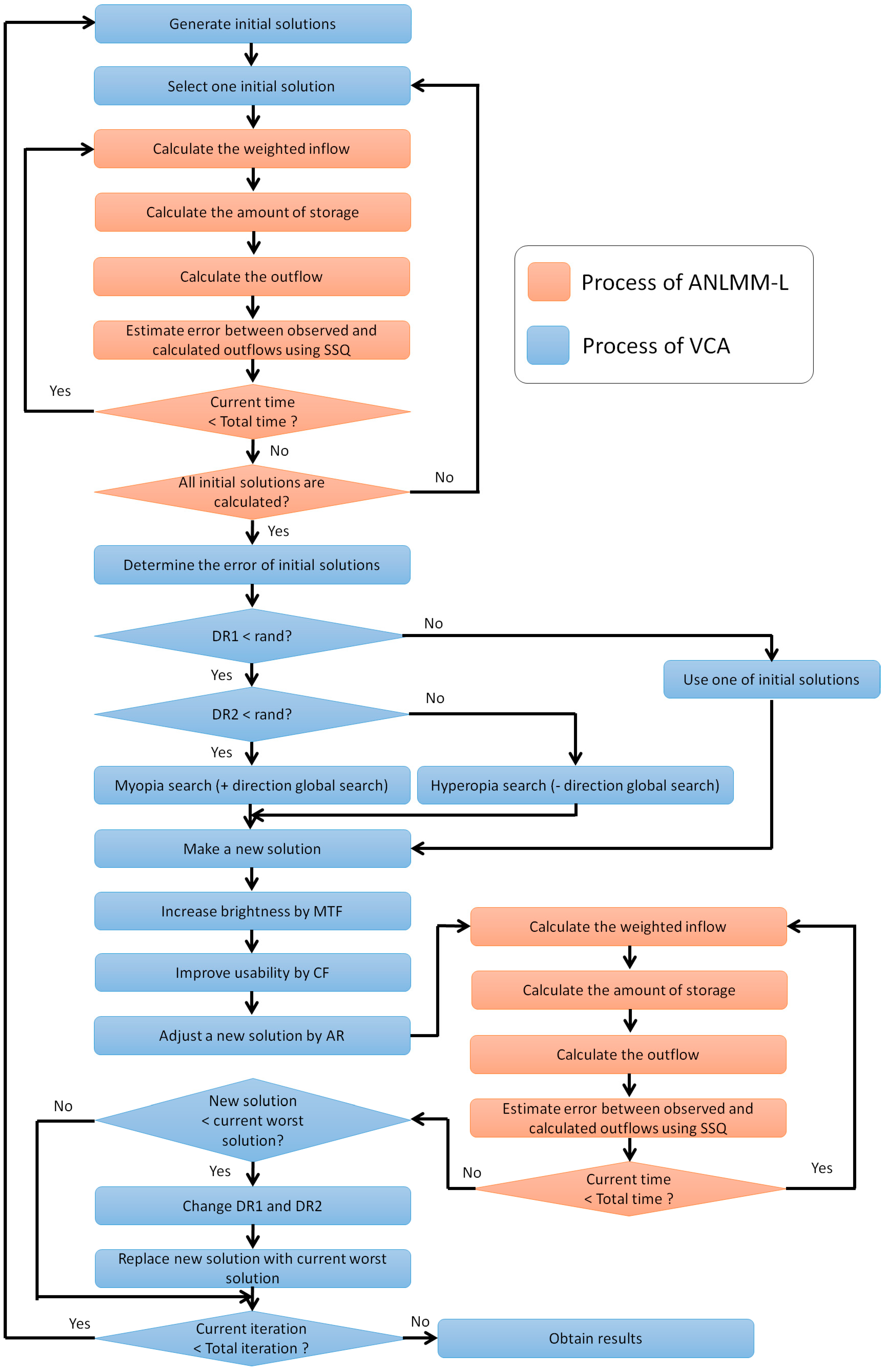
There are two procedures for the metaheuristic optimization algorithm (VCA) and new Muskingum flood routing model (ANLMM-L). In this process, the error metrics are the objective functions in optimization algorithms. This means that the error between observed and simulated flood data is minimized by the selected optimization algorithm. This is the method to code the computation process of ANLMM-L and to minimize the error using VCA. Initial solutions for parameters of ANLMM-L are generated and one initial solution is selected in the process of VCA. Then, the weighted inflow, amount of storage, and outflow are continuously calculated. The error between observed and calculated outflows using the sum of squares (SSQ) is estimated until total time.
If all initial solutions are calculated by the process of ANLMM-L, the error of initial solutions is determined and those are sorted by the error of initial solutions. It is determined whether to produce a new solution by global search, or select one of the initial solutions according to the division rate 1 (DR1). The global search direction is determined according to the division rate 2 (DR2). A new solution is generated and it is modified by modulation transfer function (MTF), compression factor (CF), astigmatic rate (AR).
Then, the process of ANLMM-L for a new solution is applied. The weighted inflow, amount of storage, and outflow are continuously calculated to estimate error between observed and calculated outflows using SSQ until total time. If the error of the new solution is smaller than it of the current worst solution, the new solution is replaced with the current worst solution and DR1/DR2 are changed. All this process is repeated until total iteration. The flowchart for the calculation of ANLMM-L and VCA is shown in Figure 1.
2.2. Advanced Nonlinear Muskingum Model Considering Continuous Flow
The initial flood routing procedure of NLMM-L was suggested by considering the current time inflow. Equation (1) was suggested for the calculation of outflow [5,7].
where Ot is the amount of outflow (m3/s) and χ is a weighting factor. St is the amount of storage (m3/s) and m is a parameter accounting for the nonlinearity of flood wave behavior. K is the storage factor, β is the factor for lateral flow, and It is the amount of inflow (m3/s). The current inflow with four parameters (K, χ, m, β) is included in this equation. Additionally, a method for considering the lateral flow with the previous inflow was proposed. The current inflow and the previous inflow are weighted to calculate the inflow. The calculation of weighted inflow is shown in Equation (2).
where Wt is the weighted inflow (m3/s), θ is the weighted factor, and It−1 is the amount of previous inflow (m3/s). The weighted inflow considering the current and previous inflows has five parameters (K, χ, m, β, θ) for the calculation of outflow. Equation (3) was suggested for the calculation of outflow using the current and previous inflows [14].
where K is the coefficient of storage (days). The time interval of the recorded measurements and the length of the investigated reach (that is linked to the wave travel time from the upstream section to the downstream section) are very important for the effect of the inflow at each time. The time interval of the recorded measurements is considered during the calculation of St (amount of storage) because the calculation of St includes the time interval. Equation (4) shows the equation of state using the continuity equations.
where St+1 is the amount of storage when the time is t + 1 (m3/s·day) and St is the amount of storage when the time is t (m3/s·day). It is the amount of inflow (m3/s) and Ot is the amount of outflow (m3/s). The length of the investigated reach is considered by the parameters of the weighted inflow. If the length of the investigated reach is long, the effects of inflows at previous time will be decreased. Conversely, if the length of the investigated reach is short, the effects of inflows at previous time will be increased.
This Muskingum routing method was applied to five flood data (Wilson flood data, flood data by Wang et al. [10], flood in the River Wye December, Sutculer flood, flood in River Wyre October). Four out of five results show that parameter θ is 0 (Wilson flood data, flood in the River Wye December, flood in River Wyre October) or 1 (Sutculer flood). This indicates that the previous and current inflows are only considered when θ is 0 and 1, respectively. A new method is required to overcome this phenomenon because these results show that both previous and current inflows is not fully applied to NLMM-L.
ANLMM-L in this study is suggested to improve NLMM-L by considering three types of inflows: first previous, second previous, and current inflows. Equation (5) shows the calculation of the new weighted inflow.
where θ1 is the weighted factor of the first previous inflow, θ2 is the weighted factor of the second previous inflow, and It−2 is the amount of second previous inflow (m3/s). The weighted inflow including first previous, second previous, and current inflows has six parameters (K, χ, m, β, θ1, θ2) for the calculation of outflow. Equation (3) in NLMM-L is also used for the calculation of outflow of ANLMM-L. The original Muskingum flood routing model perfectly preserves mass balance. Conversely, the Muskingum-Cunge (MC) contains a loss of mass because it increases with the flatness of the bed slope, reaching values of 8 to 10% at slopes of 10−4 [15]. The concept of ANLMM-L perfectly contains the mass conservations because it is based on Muskingum flood routing model.
2.3. Numerical Method for Parameter Estimation
The range of parameters is an important factor in the Muskingum flood routing model. The range of most parameters in ANLMM-L is equal to that in NLMM-L because ANLMM-L is a modified version of NLMM-L. The ranges of six parameters for ANLMM-L are given in Table 1.
The SSQ was applied to calculate the error values in each Muskingum flood routing method [8]. The SSQ of the difference between the observed and calculated outflows was used as an objective function. The six parameters (K, χ, m, β, θ1, θ2) were used as decision variables in the objective function. The objective function in ANLMM-L is shown in Equation (6).
where Oobs is the amount of observed outflow (m3/s) and Ocal is the amount of calculated outflow (m3/s). The root mean square error (RMSE) and Nash-Sutcliffe efficiency (NSE) as well as SSQ were added to compare the performance of the different models. The function of RMSE is shown in Equation (7).
where x1 is the amount of observed outflow (m3/s), x2 is the amount of calculated outflow (m3/s), and n is the number of data. The function of NSE is shown in Equation (8).
where x1 is the amount of observed outflow (m3/s), x2 is the amount of calculated outflow (m3/s), is the amount of average outflow (m3/s) and n is the number of data. The results of kinematic wave model (KWM), linear Muskingum method (LMM), linear Muskingum method incorporating lateral flow (LMM-L), nonlinear Muskingum method (NLMM), NLMM-L, and ANLMM-L are compared for verifying the effectiveness of ANLMM-L.
2.4. Vision Correction Algorithm
VCA, whose development was inspired from a vision correction procedure, was applied to several mathematical benchmark problems such as Rosenbrock’s valley, Easom, Goldstein price, Rastrigin, Griewank, and Ackley for verifying its performance [16]. VCA based on the optical characteristics for vision correction is inspired by the process of human vision. VCA includes several parameters such as DR1, DR2, modulate transfer function rate (MR), and AR. The process of VCA consists of several steps: (1) Generate initial solutions; (2) Generate a new solution (DR1 and DR2); (3) Apply MR and AR; (4) Replace the current worst solution with a new solution if the new solution is better than the current worst solution.
The initial solutions are randomly generated between the upper and lower boundaries. Each decision variable has a range and is determined within this range. A new solution can be generated in the selection of current solutions or random generation. In the selection of current solutions, each decision variable is chosen with a given probability according to the value of fitness. Random generation has two kinds of search directions: positive direction and negative direction. The new decision variable is searched in the positive direction (from the best decision variable to the upper boundary) when it is a myopia (nearsighted). In contrast, the new decision variable is determined in the negative direction (from the lower boundary to the best decision variable) when it is a hyperopia (farsighted). Equation (9) shows the generation of new decision variables.
where nx is the new decision variable, bx is the current best decision variable, and random (0, 1) is a random value from 0 to 1. The terms ub and lb indicate the upper and lower boundaries, respectively. The process of MR is applied after the generation of new decision variables. In this process, the concept of MTF is based on the distance between the decision variable of the current best solution and the new decision variable. Additionally, each decision variable has a different value of MTF. Equation (10) shows the calculation of MTF.
where MTFj is the value of MTF of the j-th decision variable and k is the total number of decision variables. dxj represents the distance ratio between A (xi − x1) and B (xn − x1) at the j-th decision variable (A: distance from the selected decision variable (xi) to the best decision variable (x1); B: distance from the worst decision variable (xn) to the best decision variable). Each decision variable is adjusted using the MR process as given in Equation (11).
where random (−1, 1) is a random value from −1 to 1 and CF is a compression factor between 0 and 100. The process of AR inspired by an astigmatic correction is used after the application of MR. The astigmatic correction of vertical and horizontal errors is conducted to view three-dimensional objects. Each decision variable is calculated using the AR process as given in Equation (12).
where ϕ is the astigmatic angle (AF). After all the processes including MR and AR are completed, the new solution with new decision variables is compared with the current worst solution. The current worst solution is replaced with the new solution if the new solution is better than the current worst solution. Five parameters—candidate glasses (CG), MR, CF, AR, and AF—were used in VCA. CG is the number of initial solutions and MR is the probability of the MR process. CF is the factor that reduces the local search range. AR is the probability of the AR process and AF is the astigmatic angle used in the AR process. The ranges of each parameter in VCA are selected as [10, 500] for CG, [0, 1] for MR, [0, 100] for CF, [0, 1] for AR, and [0, 180] for AF. The pseudo-code of VCA is presented in Table 2.
The number of function evaluations (NFEs) was used in the optimization process instead of the total iteration number. The NFE is the product of the number of new solutions in each iteration and the total iteration number. NFE was considered as 100,000 in all the flood data. The VCA used as an optimization technique has five parameters (CG, MR, CF, AR, and AF). The values of the five parameters are selected as 50, 0.1, 2, 0.1, and 45 for CG, MR, CF, AR, and AF, respectively, in all applications. The application procedure of ANLMM-L using VCA as follows:
- Generate initial solutions
- Calculate the fitness of solutions using the objective function
- Generate new solution
- Compare new solution with current worst solution
- Determine the replacement between two solutions
- Repeat steps 2–5 if iteration process is not finished.
The optimization algorithms in Muskingum routing models are only tools for quickly finding the optimum value and does not improve the optimum value. The results of all Muskingum routing models using optimization algorithms are based on the performance of each Muskingum routing model. The ANLMM-L will show the same results if other optimization algorithm are applied instead of VCA. The VCA was used in ANLMM-L and it is a kind of meta-heuristic optimization technique. Therefore, the VCA can be applied to a distributed model structure in which many spatial discretizations are used.
The choice of optimization algorithm is not an important issue in this study. It is also possible to select other optimization algorithms because the optimization in this study is only a tool for accurate Muskingum flood routing. The choice of optimization algorithms is not a problem if the proper parameters in Muskingum flood routing models can be selected. The purpose of this study is the prediction of the accurate outflows using one of optimization algorithms. The VCA has the advantage of finding the correct solutions; however, it is difficult to calibrate, because the VCA has many parameters.
3. Results
3.1. Application of Wilson Flood Data
The Wilson flood data were used in 1974 and the parameter estimation was conducted using the cuckoo search algorithm (CSA) [8]. The LMM-L [3], NLMM [17], and NLMM-L [8] were applied to the Wilson flood data. The optimal parameters of NLMM-L for the Wilson flood data were determined to be 0.5342 for K, 0.3005 for χ, 1.8642 for m, −0.0216 for β, and 0.0000 for θ using CSA [8]. The reason for choosing these values is that the value of θ becomes 0, and only the previous inflow is included in the calculation of outflow. The optimal parameters of ANLMM-L for the Wilson flood data were determined to be 0.933576 for K, 0.340998 for χ, 1.746706 for m, −0.020975 for β, 0.670453 for θ1, and 0.261739 for θ2 using VCA.
The VCA was applied to the LMM-L, NLMM, NLMM-L, and ANLMM-L for the comparison of computational time in each model. All results of average computational time are based on the average value of 20 simulations with 100,000 iterations. The results of average computational time for the Wilson flood data using VCA is shown in Table 3.
In Table 3, the average computational time at three measures (SSQ, RMSE and NSE) were estimated. The computational time of SSQ is shorter than other measures (RMSE and NSE) because the structure of the equation in SSQ is simple. The computational time of RMSE is shorter than NSE because the denominator of RMSE is the number of data and it of NSE should be calculated. The average computational time of LMM-L is shorter than other models because its equation is the simplest. The computational time increases greatly when the calculating process is added. It increases a little when additional variable was added. There are differences depending on the type of Muskingum flood routing and measures for error. The proper Muskingum flood routing model should be selected according to the accuracy of results because the computational time difference between each model is not huge. The results of LMM-L, NLMM, NLMM-L, and ANLMM-L are listed in Table 4.
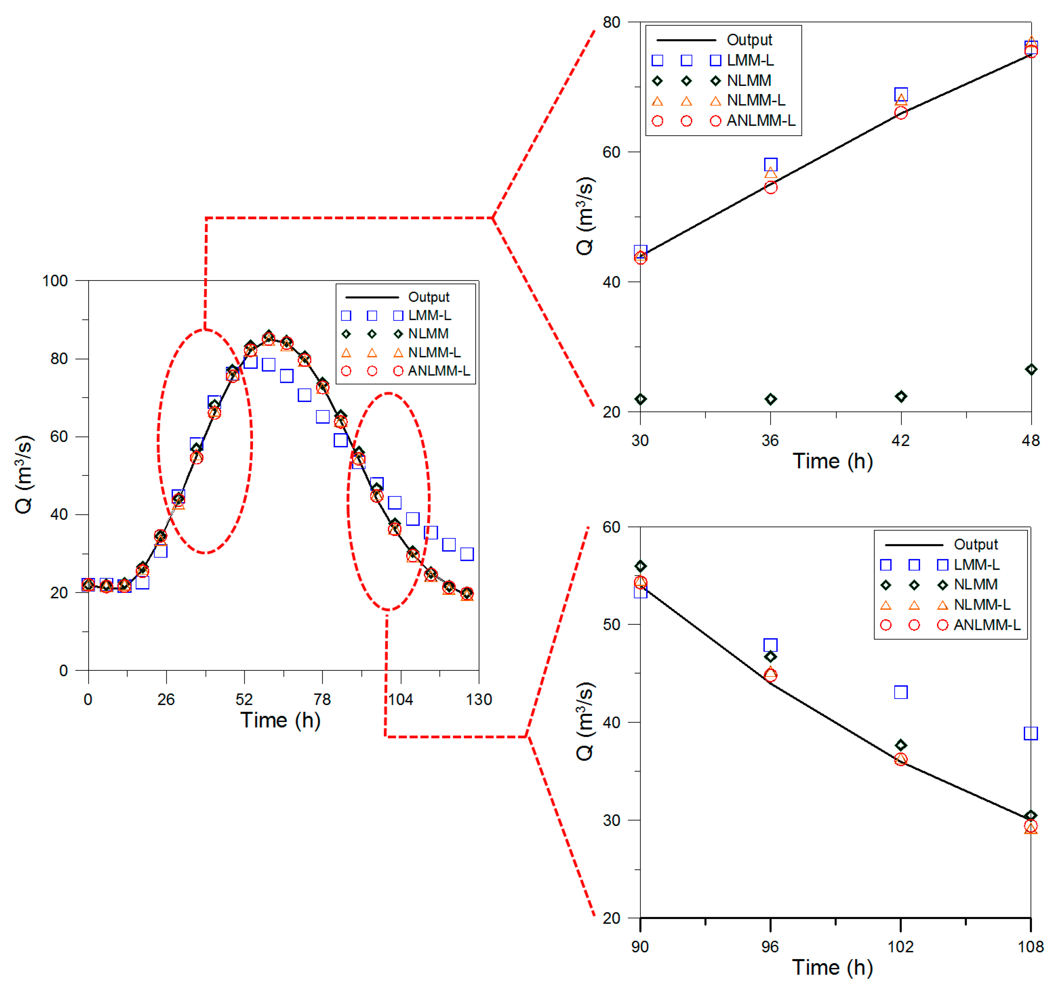
All the outflows at 0 h are equal to 22 m3/s, but the difference appears at 6 h. The values of outflow for LMM-L, NLMM, NLMM-L, and ANLMM-L are 22.1 m3/s, 22 m3/s, 21.71 m3/s, and 21.57 m3/s when the time is 6 h, respectively. The difference between the observed outflows and those calculated using each Muskingum method is apparent at 42 h although the error is larger or smaller at all times. The outflow for LMM-L, NLMM, NLMM-L, and ANLMM-L is 68.9 m3/s, 68.1 m3/s, 66.67 m3/s, and 66.01 m3/s when the observed outflow (output) at 42 h is 66 m3/s, respectively. The difference between the observed outflows and those calculated using LMM-L, NLMM, NLMM-L, and ANLMM-L is 2.9 m3/s, 2.1 m3/s, 0.67 m3/s, and 0.01 m3/s, respectively. The result obtained using ANLMM-L is better than those obtained using the other methods and this method shows the smallest value of SSQ, RMSE, and NSE. Figure 2 shows the comparison of results for the Wilson flood data.
In Figure 2, the results of LMM-L, NLMM, NLMM-L, and ANLMM-L were compared with the outflow data. The hydrograph of ANLMM-L and the hydrograph of outflow are very similar because the difference between the observed and calculated outflows at each time is less than 1 m3/s. This result shows that the ANLMM-L is much better than the previous models when applied to the Wilson flood data.
3.2. Application of Flood Data by Wang et al. (2009)
The flood data by Wang et al. [10] were used for the application of the hybrid genetic algorithm. The LMM [10], NLMM [14], and NLMM-L [8] were applied to the flood data by Wang et al. [10]. The optimal parameters of NLMM-L for the flood data by Wang et al. [10] were determined to be 0.2179 for K, −1.1304 for χ, 1.2207 for m, −0.0024 for β, and 0.7999 for θ using CSA [8]. The reason for choosing these data is different from that of choosing the Wilson flood data as the value of θ is not 0. The reason for selecting these data is to verify whether the ANLMM-L exhibits good performance even in the case where the NLMM-L operates without difficulties. The optimal parameters of ANLMM-L for the flood data by Wang et al. [10] were determined to be 0.178058 for K, −1.49182 for χ, 1.235281 for m, −0.00243 for β, 0.268097 for θ1, and 0.0384045 for θ2 using VCA. The results of LMM-L, NLMM, NLMM-L, and ANLMM-L are listed in Table 5.
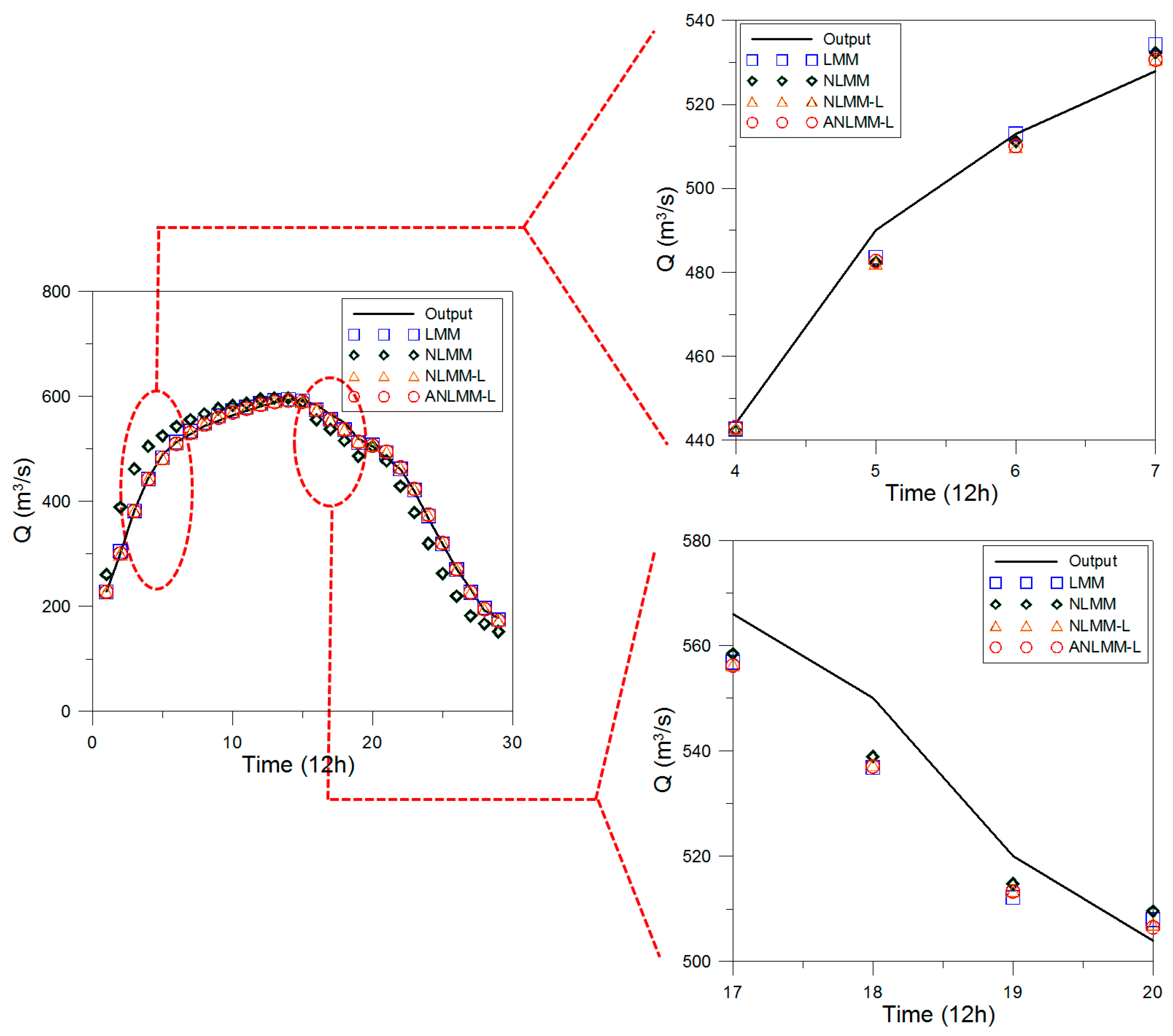
All the outflows at 12 h are equal to 228 m3/s and the initial difference between the observed outflows and those calculated using NLMM-L at 24 h is smaller than the corresponding value for the other methods. However, the magnitude of the difference between the observed and calculated outflows varies at each time. The ANLMM-L generally shows better results than the other methods although there is no significant difference at each time. Figure 3 shows the comparison of results for Wang et al.’s data [10].
The outflows of LMM-L, NLMM, NLMM-L, and ANLMM-L were compared with the output in Figure 3. In Wang et al.’s flood data [10], the hydrograph of outflow using ANLMM-L is slightly different from that of the output because the difference between the observed and calculated outflows occasionally exceeds 10 m3/s. The SSQ of ANLMM-L is better than that of the other methods with Wang et al.’s flood data [10].
3.3. Application of Flood Data for River Wye December in 1960
The River Wye, UK, with no tributaries, is linked from Erwood to Belmont; its total length is 69.75 km. The flood data for River Wye December in 1960 were suggested for the application of flood routing methods [11]. The LMM-L [4], NLMM [17], and NLMM-L [8] were applied to the flood data for River Wye December in 1960. The optimal parameters of NLMM-L for the flood data of River Wye December in 1960 were determined to be 0.3691 for K, 0.3830 for χ, 1.6141 for m, 0.0547 for β, and 0.0000 for θ using CSA [8]. The reason for choosing these data is to enable the comparison between ANLMM-L and the other methods to verify the improvement in flood routing owing to the new method for large outflows. The optimal parameters of ANLMM-L for the flood data of River Wye December in 1960 were determined to be 1.000000 for K, 0.473018 for χ, 1.478194 for m, 0.057214 for β, 0.799610 for θ1, and 0.212095 for θ2 using VCA. The results of LMM-L, NLMM, NLMM-L and ANLMM-L are listed in Table 6.
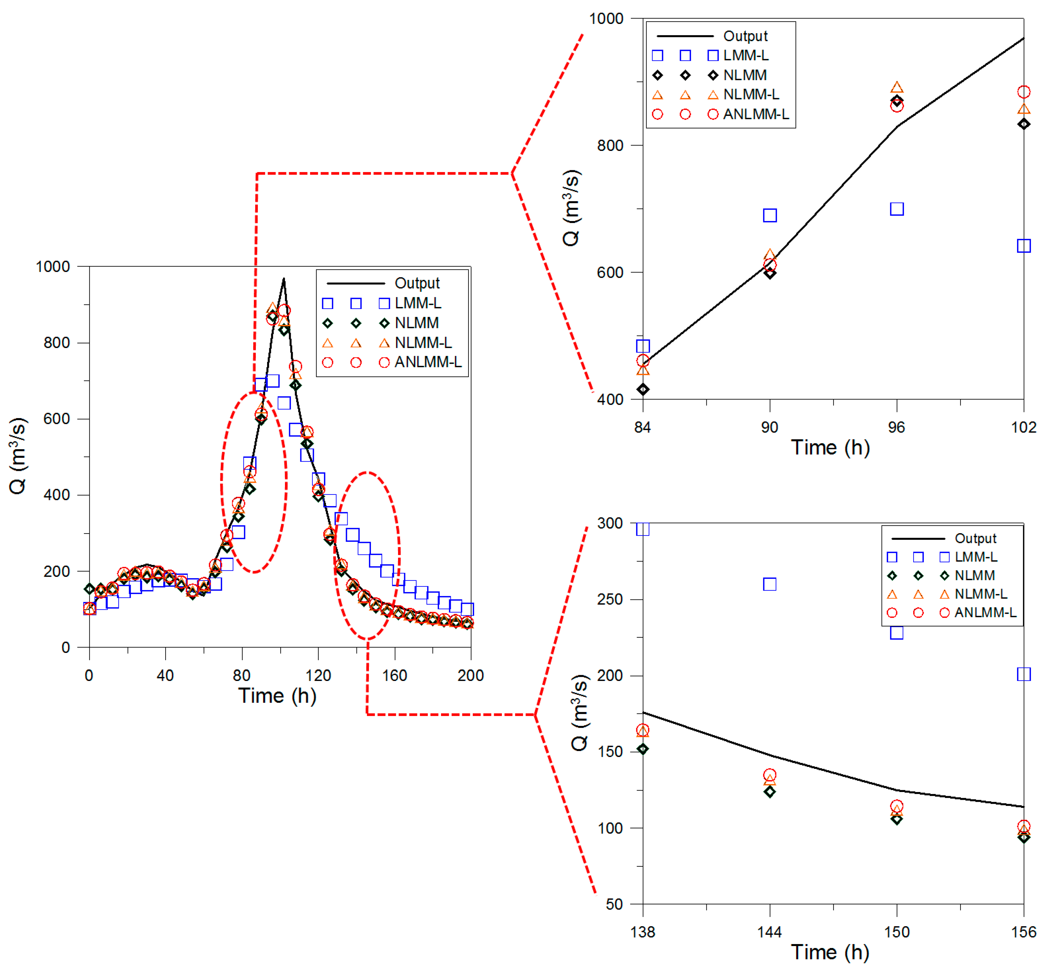
All the outflows at 0 h are equal to 102 m3/s except for that of NLMM (152 m3/s). The difference between the observed outflows and those calculated using ANLMM-L at 102 h is noticeably smaller than those of the other methods. The outflow of LMM-L, NLMM, NLMM-L, and ANLMM-L is 642 m3/s, 834 m3/s, 859.01 m3/s, and 884.60 m3/s when the observed outflow (output) at 102 h is 969 m3/s, respectively. The difference between the observed and calculated outflows of LMM-L, NLMM, NLMM-L, and ANLMM-L is 327 m3/s, 135 m3/s, 109.99 m3/s, and 84.40 m3/s, respectively. The result obtained using ANLMM-L is better than those obtained using the other methods and this method shows the smallest value of SSQ, RMSE, and NSE. Figure 4 shows the comparison of results for flood data of River Wye December in 1960.
In Figure 4, the outflows of LMM-L, NLMM, NLMM-L, and ANLMM-L were compared with the output for the River Wye December in 1960. The hydrograph of outflow using ANLMM-L is almost the same as the output, because the difference between the observed and calculated outflows is less than 100 m3/s. The ANLMM-L shows better performance than the other methods with the flood data of River Wye December in 1960.
3.4. Application of Sutculer Flood Data
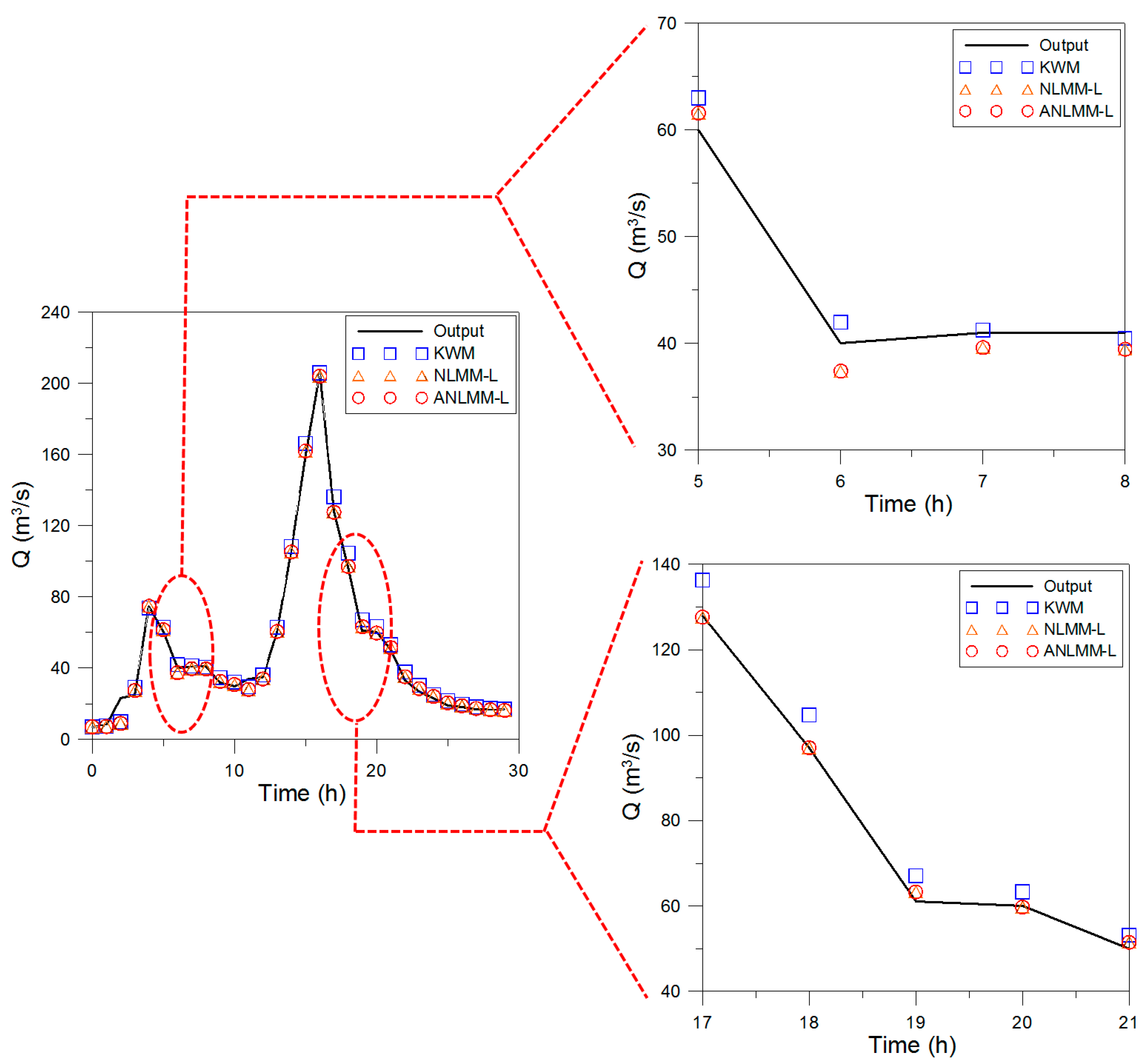
The Sutculer flood data on 4 November 1995 were recorded in Sutculer City, Turkey; it was suggested for the application of flood routing methods [12]. The kinematic wave model (KWM) was applied to the Sutculer flood data [13] and NLMM-L was compared with KWM [8]. The optimal parameters of NLMM-L for the Sutculer flood data were determined to be 0.9953 for K, −0.0196 for χ, 1.0029 for m, −0.0410 for β, and 1.0000 for θ using CSA [8]. The reason for choosing these data is to enable the comparison between ANLMM-L and the other methods. The optimal parameters of ANLMM-L for the Sutculer flood data were determined to be 0.973098 for K, −0.03454 for χ, 1.00263 for m, −0.04106 for β, 0.120753 for θ1, and 0.295127 for θ2 using VCA. The results of KWM, NLMM-L and ANLMM-L are listed in Table 7.
The difference between observed data and all simulated results becomes clear from 2 h. The peak time in all results is 16 h and the KWM has the most accurate result in the peak outflow. However, the results of KWM is larger than the observed data in the latter half. Conversely, the results of NLMM and ANLMM-L are smaller than the observed data in the first half. The result obtained using ANLMM-L is better than those obtained using the other methods and this method shows the smallest value of SSQ. The results of ANLMM-L is similar with those of NLMM-L in RMSE and NSE because the values of RMSE and NSE are smaller than those of SSQ. Figure 5 shows the comparison of results for Sutculer flood data.
In Figure 5, the outflows of KWM, NLMM-L, and ANLMM-L were compared with output for Sutculer flood data. The ANLMM-L shows better performance than the other methods with Sutculer flood data though the results of ANLMM-L are not much different from those of NLMM-L.
3.5. Application of the Flood Data for River Wyre October in 1982
In the River Wyre, flood occurred in October, 1982 and it was used for LMM-L [4]. Additionally, NLMM-L was applied to the flood data of River Wyre October in 1982 and compared with LMM-L [8]. The optimal parameters of NLMM-L for the flood data of River Wyre October in 1982 were determined to be 5.6765 for K, 0.2271 for χ, 0.9800 for m, 2.5298 for β, and 0.0000 for θ using CSA [8]. These data were chosen because these data have a multi-peak inflow. The optimal parameters of ANLMM-L for the flood data of River Wyre in October, 1982 were determined to be 6.129198 for K, 0.256363 for χ, 0.967245 for m, 2.532946 for β, 0.999999 for θ1, and 0.114425 for θ2 using VCA. The results of LMM-L, NLMM-L and ANLMM-L are listed in Table 8.
The difference between observed data and all simulated results becomes clear from 2 h. The outflow of LMM-L, NLMM-L, and ANLMM-L is 8.1 m3/s, 8.79 m3/s, and 9.94 m3/s when the observed outflow (output) at 2 h is 9.9 m3/s, respectively. The maximum error of ANLMM-L in each time does not exceed 4 unlike LMM-L and NLMM-L. Figure 6 shows the comparison of results for the flood data of River Wyre October in 1982.
In Figure 6, the outflows of LMM-L, NLMM-L, and ANLMM-L were compared with the output for the flood data of River Wyre October in 1982. The results of ANLMM-L is better than those of other models in SSQ, RMSE, and NSE. Additionally, the ANLMM-L shows better performance than the other models for the flood data of River Wyre October in 1982 because the maximum errors at each time using LMM-L, NLMM-L, and ANLMM-L are approximately 9.00 m3/s, 4.29 m3/s, 3.45 m3/s, respectively. The ANLMM-L was applied to the five flood data including the Wilson flood data, Wang et al.’s data [10], and the flood data of River Wye December in 1960, Sutculer flood data, and the flood data of River Wyre October in 1982 for overcoming the shortcoming of NLMM-L. It shows better results than other Muskingum flood routing methods (KWM, LMM, LMM-L, NLMM, and NLMM-L). Accurate Muskingum flood routing using ANLMM-L is possible for various flood data.
3.6. Application for the Prediction in Daechung Flood Data
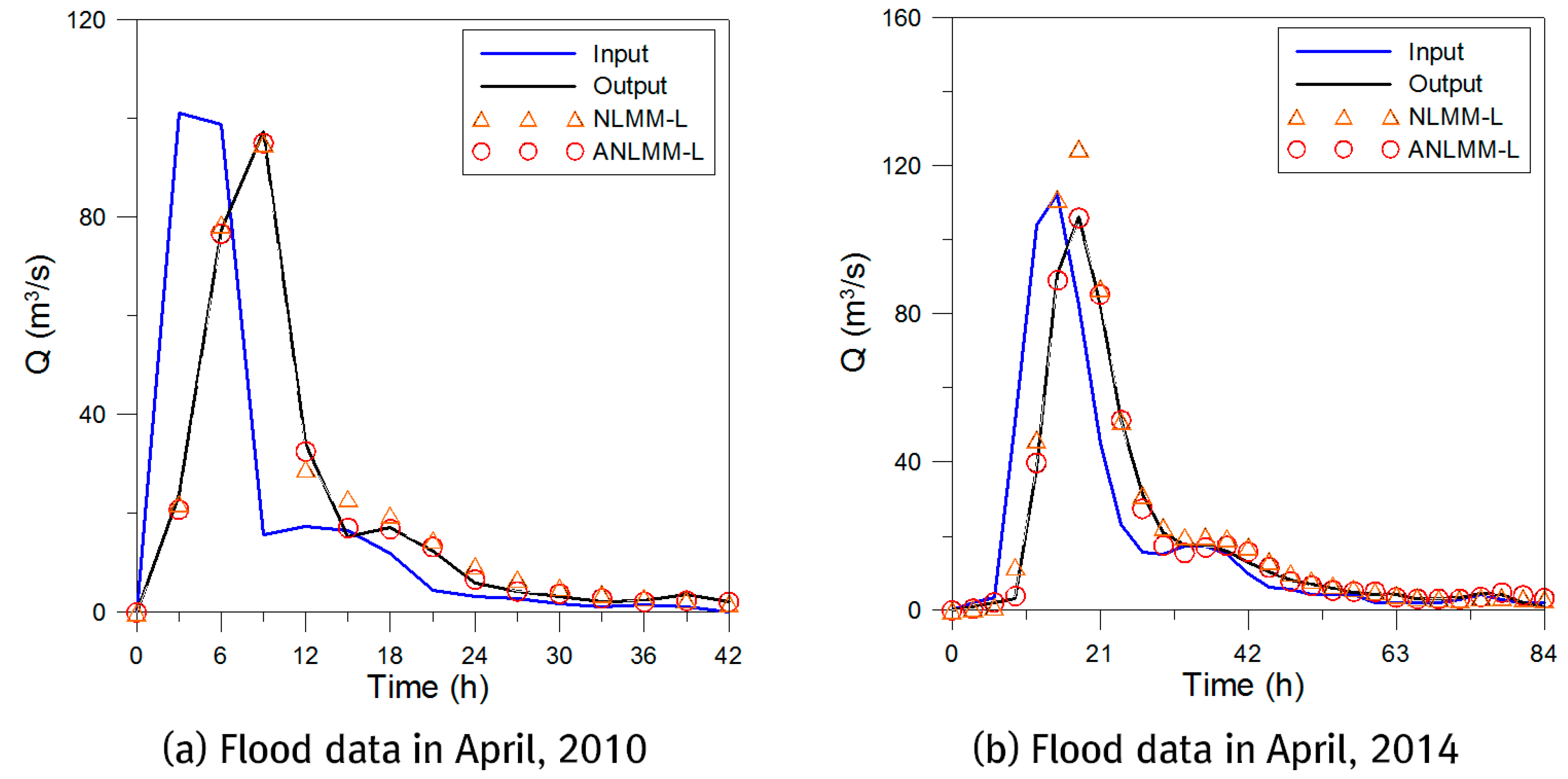
The ANLMM-L was applied to the Daechung flood data for the prediction of flood data. Daechung is the dam of Geum River in Chungcheongbuk-do, Korea. All flow data of rivers in Korea were provided by Han River Flood Control Office in Ministry of Construction and Transportation [18]. Initially, the ANLMM-L was applied to the Daechung flood data in April, 2010. The optimal parameters of ANLMM-L for the Daechung flood data in April, 2010 were determined to be 96.44027 for K, −0.47211 for χ, 7.883545 for m, 1.96461 for β, 0.78404 for θ1, and 0.21141 for θ2 using VCA. The optimal parameters of NLMM-L for the Daechung flood data in April, 2010 were determined to be 15.88463 for K, −0.23059 for χ, 0.68005 for m, 0.16082 for β, and 0.00000 for θ using VCA. Additionally, the ANLMM-L and NLMM-L were applied to the Daechung flood data in April, 2014 for the prediction of outflow. The parameters of ANLMM-L and NLMM-L for the Daechung flood data in April, 2014 were same with those for the Daechung flood data in April, 2010. The results of prediction are shown in Figure 7.
In Figure 7a, the parameter estimation was conducted with Daechung flood data in April, 2010. The results of error in 2010 were 67.60 (SSQ), 1.553773 (RMSE), and 0.997410 (NSE) using ANLMM-L. The results of error in 2010 were 131.6704 (SSQ), 2.168528 (RMSE), and 0.991726 (NSE) using NLMM-L. In Figure 7b, the same parameters were applied to the Daechung flood data in April, 2014 for the prediction of outflow. The results of error in 2014 were 23.93 (SSQ), 0.924386 (RMSE), and 0.998497 (NSE) using ANLMM-L. The results of error in 2014 were 981.20 (SSQ), 5.919692 (RMSE), and 0.962401 (NSE) using NLMM-L. It means that the ANLMM-L is significantly better than the NLMM-L in some flood data. The results of Daechung flood data show that the new method is required for accurate flood routing in real applications. The ANLMM-L can be useful for the prediction of outflow although the value of error slightly increased.
4. Discussion
The NLMM-L was suggested by the integration of the continuity and storage equations with the assumptions of O’Donnell’s nonlinear Muskingum model considering the lateral flow. The NLMM-L had a limitation, in that the weighted inflow was sometimes determined to be one of the two inflows (previous and current inflows). The most remarkable change in the new method is a new weighted inflow considering three types of inflows: the first previous, second previous, and current inflows. The two previous inflows (the first and second previous inflows) are proposed for the application of flood data, because the water flow is continuous. The weights of each inflow are determined according to two kinds of weighted factors. The outflow in Muskingum routing model should be determined by various inflows including the current inflow, first previous inflow and second previous inflows, because the outflow is affected by the continuous inflow. The ANLMM-L is applied to the Wilson flood data, the flood data by Wang et al. [10], the flood data of River Wye December in 1960, Sutculer flood data in Turkey, and the flood data of River Wyre Octorber in 1982 for the comparison between the previous and new Muskingum flood routing methods.
There is not much difference in each Muskingum flood method in five flood data. In particular, the difference between ANLMM-L and NLMM-L is not large for each flood data though the results of ANLMM-L are slightly better than those of NLMM-L. The reason for this is that one flood data is used for parameter adjustment in Muskingum flood routing methods. The parameters should be applicable to future flood data in the same place. The Daechung flood data was selected to verify two Muskingum flood routing models (NLMM-L and ANLMM-L) showing the closest results in five flood data. There was no significant difference in 2010 flood data for parameter validation, but there was large difference in 2014 flood data. Typically, there is a difference of the RMSE values by two Muskingum flood routing models. The values of RMSE in 2010 flood data are approximately 1.55 and 2.17, respectively. The difference between the two values is approximately 0.6. However, the values of RMSE in 2014 flood data are approximately 0.92 and 5.92, respectively. The RMSE value using NLMM is larger than six times of the RMSE value using ANLMM-L. This result implies that the new method can show better results as one of Muskingum flood routing models for predicting future flood data.
It can be used for more accurate flood routing and can be combined with various optimization algorithms that are easily applicable to users. In Muskingum routing models including ANLMM-L, it is not possible to estimate water level if a rating curve or river geometry is not present at a specific target point. However, such information is crucial in flood forecasting or design of hydraulic structures. The ANLMM-L does not provide more information than hydraulic flood routing models because it is a hydrologic flood routing model. The ANLMM-L was developed to estimate accurate flood routing using selected parameters based on observed flood data in a target area. The ANLMM-L is useful for flood forecasting in urban areas that have only flow information.
5. Conclusions
The Muskingum flood routing model is widely known for its simplicity, and it has been used by many water managers. The ANLMM-L can be also used for water managers that can use the original Muskingum flood routing model. The ANLMM-L has simplicity, and improves the accuracy of flood routing compared to the conventional Muskingum flood routing models. The ANLMM-L was suggested for accurate flood routing. The NLMM-L with the weighted inflow including the previous and current inflows was suggested [8].
The ANLMM-L was applied to the Wilson flood data, Wang et al.’s data [10], River Wye December in 1960, Sutculer flood data, and flood data of River Wyre October in 1982 for the comparison of new and other models. Three measures for the comparison are SSQ, RMSE, and NSE. Among three measures, SSQ was selected as the objective function in order to clearly distinguish between each Muskingum flood routing model because it shows the largest value in the application of each flood data. In the Wilson flood data, the SSQ of ANLMM-L is 4.530563 and it is the smallest value in applied Muskingum flood routing models. Additionally, The RMSE and NSE of each model showed differences. In Wang et al.’s data [10], the ANLMM-L shows better results than other models and the SSQ value of ANLMM-L was 909.2069. The SSQ values of each model showed a difference but RMSE and NSE values did not differ greatly. The ANLMM-L was compared with other models for the River Wye December in 1960. The error values in this flood data was the largest among all flood data. The SSQ value of ANLMM-L was 20,495.98 and it is the smallest value in all models. A clear difference was found in all error measures for applied Muskingum flood routing models. In Sutculer flood data, NLMM-L and ANLMM-L showed similar values. The Sutculer flood data has two peak values, and it can be seen that the ANLMM-L cannot show excellent results. In the case of Sutculer flood data with two peak outflows, the Muskingum flood routing model considering continuous inflows (ANLMM-L) cannot show better performance than NLMM-L because the value of outflow does not increase or decrease continuously. The SSQ value of ANLMM-L was 281.05 and it is similar to the SSQ value of NLMM-L, 281.11. Finally, the ANLMM-L was applied to the flood data of River Wyre October in 1982. The SSQ value of ANLMM-L is the smallest value (40.2099) in applied Muskingum flood routing models. The difference in RMSE was no large but perceivable and the difference in NSE was very small.
Daechung flood data were selected for the prediction of outflow, which is the purpose of this study. The ANLMM-L and NLMM-L, which showed the closest results in the five flood data, were applied to Daechung flood data in 2010 to estimate the parameters. Then, the prediction of outflow for Daechung flood data in 2014 was conducted by applying the same parameters for each model. There was slight difference in the process of parameter estimation, but there was big difference in the prediction of outflow. In 2014, the SSQ value of ANLMM-L was 23.93 and it of NLMM-L was 981.20. These results show that the accurate flood prediction is possible in Daechung flood data by ANLMM-L. Additionally, the ANLMM-L can be applied to the prediction of outflow in other areas.
Comprehensively, the ANLMM-L using VCA shows good results for all the flood data. The ANLMM-L, as a hydrologic flood routing model, is more accurate than conventional Muskingum flood routing models. In future studies, various methods for calculating the error of Muskingum flood routing can be added and used as an objective function in future studies. The VCA can be used not only for various flood routing models but also for parameter estimation of sewer network and for the optimal design of water distribution systems/urban drainage systems. The ANLMM-L can be used to predict flood in urban areas with only inflow and outflow data.
Author Contributions
E.H.L. and H.M.L. carried out the survey of previous studies. E.H.L. wrote the manuscript. E.H.L. conducted all simulations. E.H.L., J.H.K. and H.M.L. conceived the original idea of the proposed method.
Funding
This research was funded by National Research Foundation (NRF) of Korea in the Korean government (MISP) (No. 2016R1A2A1A05005306).
Acknowledgments
This work was supported by a grant from The National Research Foundation (NRF) of Korea in the Korean government (MSIP) (No. 2016R1A2A1A05005306).
Conflicts of Interest
The authors declare no conflict of interest.
Abbreviations
| ANLMM-L | Advanced nonlinear Muskingum flood routing model considering continuous flow |
| NLMM-L | Nonlinear Muskingum flood routing model incorporating lateral flow |
| VCA | Vision correction algorithm |
| SSQ | Sum of squares |
| DR1 | Division rate 1 |
| DR2 | Division rate 2 |
| MTF | Modulation transfer function |
| CF | Compression factor |
| AR | Astigmatic rate |
| RMSE | Root mean square error |
| NSE | Nash-Sutcliffe efficiency |
| KWM | Kinematic wave model |
| LMM | Linear Muskingum method |
| LMM-L | Linear Muskingum method incorporating lateral flow |
| NLMM | Nonlinear Muskingum method |
| AF | Astigmatic angle |
| CG | Candidate glasses |
| NFEs | Number of function evaluations |
| CSA | Cuckoo search algorithm |
References
- Jung, C.Y.; Jung, Y.H.; Kim, H.S.; Jung, S.W.; Jung, K.S. The estimation of parameter using Muskingum model in ank-dong river basin incorporating lateral inflow. In Proceedings of the 2008 Korea Water Resources Association Conference, Gyeongju, Korea, 17–18 May 2008. [Google Scholar]
- Kimura, T. The Flood Runoff Analysis Method by the Storage Function Model; The Public Works Research Institute, Ministry of Construction: Tsukuba, Japan, 1961. [Google Scholar]
- McCarthy, G.T. The unit hydrograph and flood routing. In Proceedings of the Conference of North Atlantic Division; US Army Corps of Engineers: Washington, DC, USA, 1938. [Google Scholar]
- O’Donnell, T. A direct three-parameter Muskingum procedure incorporating lateral inflow. Hydrol. Sci. J. 1985, 30, 479–496. [Google Scholar] [CrossRef] [Green Version]
- Tung, Y.K. River flood routing by nonlinear Muskingum method. J. Hydraul. Eng. 1985, 111, 1447–1460. [Google Scholar] [CrossRef]
- Das, A. Parameter estimation for Muskingum models. J. Irrig. Drain. E 2004, 130, 140–147. [Google Scholar] [CrossRef]
- Geem, Z.W. Parameter estimation for the nonlinear Muskingum model using the BFGS technique. J. Irrig. Drain. E 2006, 132, 474–478. [Google Scholar] [CrossRef]
- Karahan, H.; Gurarslan, G.; Geem, Z.W. A new nonlinear Muskingum flood routing model incorporating lateral flow. Eng. Optim. 2015, 47, 737–749. [Google Scholar] [CrossRef]
- Wilson, E.M. Engineering Hydrology; MacMillan Education: Hampshire, UK, 1974. [Google Scholar]
- Wang, W.; Xu, Z.; Qiu, L.; Xu, D. Hybrid chaotic genetic algorithms for optimal parameter estimation of Muskingum flood routing model. In Proceedings of the International Joint Conference on Computational Sciences and Optimization, Sanya, China, 24–26 April 2009; pp. 215–218. [Google Scholar]
- Bajracharya, K.; Barry, D.A. Accuracy criteria for linearised diffusion wave flood routing. J. Hydrol. 1997, 195, 200–217. [Google Scholar] [CrossRef]
- Ulke, A. Flood Routing Using Muskingum Method. Master’s Thesis, Suleyman Demirel University, Kaskelen, Kazakhstan, 2003. (In Turkish). [Google Scholar]
- Karahan, H.; Gurarslan, G. Modelling Flood Routing Problems Using Kinematic Wave Approach: Sutculer Example. In Proceedings of the 7th National Hydrology Congress, Isparta, Turkey, 26–27 September 2013. [Google Scholar]
- Geem, Z.W. Issues in optimal parameter estimation for the nonlinear Muskingum flood routing model. Eng. Optim. 2014, 46, 328–339. [Google Scholar] [CrossRef]
- Todini, E. A mass conservative and water storage consistent variable parameter Muskingum-Cunge approach. Hydrol. Earth Syst. Sci. 2007, 11, 1645–1659. [Google Scholar] [CrossRef] [Green Version]
- Lee, E.H.; Lee, H.M.; Yoo, D.G.; Kim, J.H. Application of a meta-heuristic optimization algorithm motivated by a vision correction procedure for civil engineering problems. KSCE J. Civ. Eng. 2017, 1–14. [Google Scholar] [CrossRef]
- Karahan, H.; Gurarslan, G.; Geem, Z.W. Parameter estimation of the nonlinear Muskingum flood-routing model using a hybrid harmony search algorithm. J. Hydrol. Eng. 2013, 18, 352–360. [Google Scholar] [CrossRef]
- Han River Flood Control Office. Available online: www.hrfco.go.kr (accessed on 30 April 2018).
Figure 1.
Flowchart for the calculation of ANLMM-L and VCA.

Figure 2.
Comparison of results for the Wilson flood data.

Figure 3.
Comparison of results for Wang et al.’s flood data [10].
Figure 3.
Comparison of results for Wang et al.’s flood data [10].

Figure 4.
Comparison of results for the flood data of River Wye December in 1960.

Figure 5.
Comparison of results for Sutculer flood data.

Figure 6.
Comparison of results for the flood data of River Wyre October in 1982.

Figure 7.
Results of prediction in Daechung flood data: (a) Flood data in April, 2010; (b) Flood data in April, 2014.
Figure 7.
Results of prediction in Daechung flood data: (a) Flood data in April, 2010; (b) Flood data in April, 2014.


Table 1.
Definition of parameters in ANLMM-L.
| Ranges of Parameters in ANLMM-L | K | χ | m | β | θ1 | θ2 |
|---|---|---|---|---|---|---|
| Wilson flood data | 0.01–1.00 | −0.50–0.50 | 1.00–3.00 | −0.10–0.10 | 0.00–1.00 | 0.00–1.00 |
| Flood data by Wang et al. [10] | 0.01–1.00 | −1.50–1.50 | 1.00–3.00 | −3.00–3.00 | 0.00–1.00 | 0.00–1.00 |
| Flood data for River Wye December in 1960 | 0.01–1.00 | −0.50–0.50 | 1.00–3.00 | −0.10–0.10 | 0.00–1.00 | 0.00–1.00 |
| Sutculer flood data | 0.01–1.00 | −0.50–0.50 | 1.00–3.00 | −0.10–0.10 | 0.00–1.00 | 0.00–1.00 |
| Flood data for River Wyre October in 1982 | 0.01–10.00 | −0.50–0.50 | 0.00–1.00 | −3.00–3.00 | 0.00–1.00 | 0.00–1.00 |
| Daechung flood data | 0.01–100.00 | −0.50–0.50 | 1.00–10.00 | −3.00–3.00 | 0.00–1.00 | 0.00–1.00 |
Table 2.
Pseudo-code of VCA.
| Objective function f(x), x = (x1, x2, …, xd)T |
| Generate initial glasses |
| While (t < Max number of iterations) |
| if (DR1 < rand) |
| ● Choose an existing glasses/generate new glasses |
| if (DR2 < rand) |
| ● Determine global search direction |
| end |
| end |
| if (new solution < current worst solution) |
| ● Replace new solution with current worst solution |
| end |
| ● Find the current best solution |
| End while |
Table 3.
Average computational time for the Wilson flood data using VCA.
| Measures | LMM-L | NLMM | NLMM-L | ANLMM-L |
|---|---|---|---|---|
| SSQ | 56 s | 63 s | 64 s | 66 s |
| RMSE | 60 s | 67 s | 68 s | 70 s |
| NSE | 68 s | 70 s | 72 s | 73 s |
Table 4.
Comparison of the outflow hydrographs calculated for the Wilson flood data.
| Time (h) | Input (m3/s) | Output (m3/s) | LMM-L (O’Donnell [4]) | NLMM (Karahan [17]) | NLMM-L (Karahan [8]) | ANLMM-L (This Study) |
|---|---|---|---|---|---|---|
| 0 | 22 | 22 | 22 | 22 | 22.00 | 22.00 |
| 6 | 23 | 21 | 22.1 | 22 | 21.71 | 21.57 |
| 12 | 35 | 21 | 21.7 | 22.4 | 22.02 | 21.67 |
| 18 | 71 | 26 | 22.6 | 26.6 | 26.08 | 25.46 |
| 24 | 103 | 34 | 30.7 | 34.5 | 33.51 | 34.59 |
| 30 | 111 | 44 | 44.7 | 44.2 | 42.83 | 43.73 |
| 36 | 109 | 55 | 58.1 | 56.9 | 55.44 | 54.59 |
| 42 | 100 | 66 | 68.9 | 68.1 | 66.67 | 66.01 |
| 48 | 86 | 75 | 76.1 | 77.1 | 75.77 | 75.52 |
| 54 | 71 | 82 | 79.2 | 83.3 | 82.12 | 82.16 |
| 60 | 59 | 85 | 78.5 | 85.9 | 84.78 | 85.04 |
| 66 | 47 | 84 | 75.6 | 84.5 | 83.42 | 84.00 |
| 72 | 39 | 80 | 70.7 | 80.6 | 79.44 | 79.62 |
| 78 | 32 | 73 | 65.1 | 73.7 | 72.48 | 72.63 |
| 84 | 28 | 64 | 59.1 | 65.4 | 64.08 | 63.80 |
| 90 | 24 | 54 | 53.4 | 56 | 54.58 | 54.31 |
| 96 | 22 | 44 | 47.9 | 46.7 | 45.22 | 44.80 |
| 102 | 21 | 36 | 43.1 | 37.7 | 36.34 | 36.25 |
| 108 | 20 | 30 | 38.9 | 30.5 | 29.21 | 29.45 |
| 114 | 19 | 25 | 35.4 | 25.2 | 24.21 | 24.63 |
| 120 | 19 | 22 | 32.3 | 21.7 | 20.96 | 21.39 |
| 126 | 18 | 19 | 29.9 | 20 | 19.41 | 19.81 |
| SSQ | - | - | 815.68 | 36.77 | 9.82 | 4.54 |
| RMSE | - | - | 6.232327 | 1.330234 | 0.683938 | 0.464948 |
| NSE | - | - | 0.965417 | 0.998424 | 0.999584 | 0.999808 |
Table 5.
Comparison of the outflow hydrographs calculated for Wang et al.’s flood data [10].
Table 5.
Comparison of the outflow hydrographs calculated for Wang et al.’s flood data [10].
| Time (12 h) | Input (m3/s) | Output (m3/s) | LMM (Wang et al. [10]) | NLMM (Geem [7]) | NLMM-L (Karahan et al. [8]) | ANLMM-L (This Study) |
|---|---|---|---|---|---|---|
| 1 | 261 | 228 | 228 | 228 | 228.00 | 228.00 |
| 2 | 389 | 300 | 305.19 | 303.8 | 299.74 | 300.92 |
| 3 | 462 | 382 | 382 | 382.3 | 382.57 | 381.51 |
| 4 | 505 | 444 | 442.7 | 442.4 | 442.76 | 443.15 |
| 5 | 525 | 490 | 483.6 | 482.4 | 482.16 | 482.69 |
| 6 | 543 | 513 | 513 | 511.2 | 509.89 | 510.09 |
| 7 | 556 | 528 | 534.29 | 532.3 | 530.72 | 530.66 |
| 8 | 567 | 543 | 550.44 | 548.5 | 546.77 | 546.62 |
| 9 | 577 | 553 | 563.53 | 561.7 | 559.96 | 559.77 |
| 10 | 583 | 564 | 573.16 | 571.6 | 569.94 | 569.80 |
| 11 | 587 | 573 | 580.02 | 578.7 | 577.07 | 576.95 |
| 12 | 595 | 581 | 587.32 | 586.2 | 584.39 | 584.22 |
| 13 | 597 | 588 | 592.14 | 591.2 | 589.68 | 589.60 |
| 14 | 597 | 594 | 594.59 | 593.9 | 592.34 | 592.30 |
| 15 | 589 | 592 | 592.02 | 591.8 | 590.33 | 590.34 |
| 16 | 556 | 584 | 574.89 | 575.7 | 574.68 | 574.86 |
| 17 | 538 | 566 | 556.85 | 558.5 | 556.41 | 556.23 |
| 18 | 516 | 550 | 536.93 | 539 | 537.43 | 537.13 |
| 19 | 486 | 520 | 512.18 | 514.8 | 513.47 | 513.35 |
| 20 | 505 | 504 | 507.96 | 509.6 | 507.07 | 506.51 |
| 21 | 477 | 483 | 493.22 | 494.9 | 494.86 | 494.95 |
| 22 | 429 | 461 | 462.34 | 464.8 | 464.39 | 464.94 |
| 23 | 379 | 420 | 421.87 | 425.1 | 423.97 | 424.15 |
| 24 | 320 | 368 | 372.34 | 376.1 | 375.05 | 375.07 |
| 25 | 263 | 318 | 318.97 | 322.4 | 321.35 | 321.35 |
| 26 | 220 | 271 | 270.39 | 272.5 | 271.42 | 271.40 |
| 27 | 182 | 234 | 226.99 | 227.5 | 226.94 | 227.09 |
| 28 | 167 | 193 | 197.2 | 195.7 | 194.92 | 195.13 |
| 29 | 152 | 178 | 174.87 | 172.6 | 172.46 | 172.76 |
| SSQ | - | - | 1086.84 | 979.96 | 917.06 | 909.35 |
| RMSE | - | - | 6.121869 | 5.820949 | 5.623120 | 5.599733 |
| NSE | - | - | 0.998180 | 0.998354 | 0.998464 | 0.998477 |
Table 6.
Comparison of the outflow hydrographs calculated for the River Wye December in 1960.
| Time (h) | Input (m3/s) | Output (m3/s) | LMM-L (O’Donnell [4]) | NLMM (Karahan et al. [17]) | NLMM-L (Karahan et al. [8]) | ANLMM-L (This Study) |
|---|---|---|---|---|---|---|
| 0 | 154 | 102 | 102 | 154 | 102.00 | 102.00 |
| 6 | 150 | 140 | 116 | 154 | 149.50 | 146.52 |
| 12 | 219 | 169 | 120 | 152 | 156.59 | 155.74 |
| 18 | 182 | 190 | 147 | 181 | 191.40 | 194.41 |
| 24 | 182 | 209 | 158 | 191 | 200.79 | 194.19 |
| 30 | 192 | 218 | 165 | 185 | 195.14 | 196.05 |
| 36 | 165 | 210 | 176 | 187 | 197.46 | 198.35 |
| 42 | 150 | 194 | 178 | 179 | 188.48 | 186.83 |
| 48 | 128 | 172 | 176 | 162 | 170.80 | 172.12 |
| 54 | 168 | 149 | 164 | 141 | 148.10 | 150.37 |
| 60 | 260 | 136 | 160 | 154 | 162.59 | 167.56 |
| 66 | 471 | 228 | 167 | 198 | 210.36 | 216.61 |
| 72 | 717 | 303 | 218 | 264 | 281.58 | 294.27 |
| 78 | 1092 | 366 | 303 | 344 | 367.75 | 378.29 |
| 84 | 1145 | 456 | 484 | 416 | 447.65 | 461.17 |
| 90 | 600 | 615 | 690 | 599 | 629.57 | 612.03 |
| 96 | 365 | 830 | 700 | 871 | 892.78 | 862.51 |
| 102 | 277 | 969 | 642 | 834 | 859.01 | 884.60 |
| 108 | 227 | 665 | 572 | 689 | 719.30 | 737.54 |
| 114 | 187 | 519 | 505 | 535 | 567.50 | 565.33 |
| 120 | 161 | 444 | 442 | 397 | 427.85 | 414.97 |
| 126 | 143 | 321 | 386 | 283 | 308.86 | 297.45 |
| 132 | 126 | 208 | 338 | 202 | 220.90 | 216.14 |
| 138 | 115 | 176 | 296 | 152 | 163.64 | 164.43 |
| 144 | 102 | 148 | 260 | 124 | 131.90 | 134.94 |
| 150 | 93 | 125 | 228 | 106 | 111.93 | 114.46 |
| 156 | 88 | 114 | 201 | 94 | 99.28 | 101.24 |
| 162 | 82 | 106 | 179 | 88 | 92.90 | 94.00 |
| 168 | 76 | 97 | 160 | 82 | 86.14 | 86.94 |
| 174 | 73 | 89 | 144 | 75 | 79.34 | 80.13 |
| 180 | 70 | 81 | 130 | 73 | 76.46 | 76.87 |
| 186 | 67 | 76 | 118 | 69 | 73.13 | 73.54 |
| 192 | 63 | 71 | 109 | 66 | 69.85 | 70.23 |
| 198 | 59 | 66 | 100 | 62 | 65.09 | 65.60 |
| SSQ | - | - | 251,802 | 37,944.15 | 25,915.27 | 20,494.98 |
| RMSE | - | - | 87.351953 | 33.900478 | 28.023846 | 24.921077 |
| NSE | - | - | 0.892983 | 0.983882 | 0.988986 | 0.991290 |
Table 7.
Comparison of the outflow hydrographs calculated for the Sutculer flood data.
| Time (h) | Input (m3/s) | Output (m3/s) | KWM (Karahan and Gurarslan [13]) | NLMM-L (Karahan et al. [8]) | ANLMM-L (This Study) |
|---|---|---|---|---|---|
| 0 | 7.53 | 7 | 7.00 | 7.00 | 7.00 |
| 1 | 9.06 | 8 | 7.62 | 7.24 | 7.26 |
| 2 | 28 | 23 | 9.98 | 9.00 | 9.01 |
| 3 | 79.8 | 25 | 29.16 | 27.35 | 27.35 |
| 4 | 64.3 | 75 | 73.78 | 74.84 | 74.81 |
| 5 | 38.2 | 60 | 63.01 | 61.57 | 61.59 |
| 6 | 41.4 | 40 | 41.98 | 37.40 | 37.41 |
| 7 | 41.3 | 41 | 41.25 | 39.63 | 39.62 |
| 8 | 33.8 | 41 | 40.48 | 39.47 | 39.47 |
| 9 | 32 | 32 | 34.64 | 32.57 | 32.58 |
| 10 | 29 | 30 | 32.13 | 30.68 | 30.68 |
| 11 | 35 | 34 | 29.52 | 28.00 | 28.00 |
| 12 | 63.1 | 35 | 36.16 | 33.93 | 33.93 |
| 13 | 110 | 60 | 62.98 | 60.62 | 60.62 |
| 14 | 170 | 105 | 108.45 | 105.25 | 105.25 |
| 15 | 216 | 160 | 166.29 | 162.06 | 162.07 |
| 16 | 131 | 206 | 206.02 | 204.11 | 204.11 |
| 17 | 101 | 128 | 136.31 | 127.58 | 127.61 |
| 18 | 65 | 97 | 104.68 | 97.14 | 97.10 |
| 19 | 62.4 | 61 | 67.14 | 63.33 | 63.32 |
| 20 | 53.8 | 60 | 63.35 | 59.78 | 59.76 |
| 21 | 36.3 | 50 | 53.18 | 51.51 | 51.50 |
| 22 | 29.6 | 33 | 37.84 | 35.16 | 35.16 |
| 23 | 25 | 27 | 30.34 | 28.49 | 28.48 |
| 24 | 21.3 | 23 | 25.11 | 24.03 | 24.03 |
| 25 | 19.6 | 19 | 21.68 | 20.49 | 20.49 |
| 26 | 18 | 18 | 19.71 | 18.81 | 18.81 |
| 27 | 17.3 | 17 | 18.1 | 17.29 | 17.29 |
| 28 | 17 | 17 | 17.39 | 16.60 | 16.60 |
| 29 | 16 | 17 | 16.97 | 16.29 | 16.29 |
| SSQ | - | - | 532.62 | 281.11 | 280.95 |
| RMSE | - | - | 4.213541 | 3.062067 | 3.060222 |
| NSE | - | - | 0.992271 | 0.995918 | 0.995923 |
Table 8.
Comparison of the outflow hydrographs calculated for the food data of River Wyre October in 1982.
Table 8.
Comparison of the outflow hydrographs calculated for the food data of River Wyre October in 1982.
| Time (h) | Input (m3/s) | Output (m3/s) | LMM-L (O’Donnell [4]) | NLMM-L (Karahan et al. [8]) | ANLMM-L (This Study) |
|---|---|---|---|---|---|
| 0 | 2.6 | 8.3 | 8.3 | 8.3 | 8.30 |
| 1 | 4.2 | 9 | 8.2 | 8.51 | 8.52 |
| 2 | 12.3 | 9.9 | 8.1 | 8.79 | 9.94 |
| 3 | 25.4 | 10.2 | 12.7 | 10.94 | 12.74 |
| 4 | 24.1 | 18.9 | 27.9 | 20.28 | 19.71 |
| 5 | 20.3 | 35.9 | 39.9 | 37.54 | 35.73 |
| 6 | 23.3 | 51.8 | 45.7 | 49.07 | 48.87 |
| 7 | 27.7 | 59.4 | 52.2 | 55.11 | 55.95 |
| 8 | 27.7 | 63.3 | 61.4 | 62.5 | 62.74 |
| 9 | 26.9 | 69.6 | 68.9 | 71.44 | 71.35 |
| 10 | 24.8 | 76.7 | 74.7 | 78.03 | 77.95 |
| 11 | 26.9 | 82 | 77.2 | 82.07 | 82.67 |
| 12 | 33.7 | 85.3 | 79.8 | 83.72 | 85.27 |
| 13 | 33.9 | 89 | 87.8 | 87.43 | 88.11 |
| 14 | 27.8 | 94.6 | 95.5 | 95.49 | 94.74 |
| 15 | 20.8 | 98.8 | 97.7 | 100.88 | 99.90 |
| 16 | 15.6 | 98 | 94.4 | 99.29 | 98.87 |
| 17 | 11.9 | 91.8 | 87.9 | 92.06 | 92.05 |
| 18 | 9.5 | 82.3 | 79.8 | 82.22 | 82.36 |
| 19 | 7.8 | 72 | 71.5 | 71.75 | 71.88 |
| 20 | 6.5 | 61.9 | 63.6 | 61.94 | 61.93 |
| 21 | 5.8 | 53 | 56.1 | 53.12 | 53.10 |
| 22 | 5.0 | 45.6 | 49.6 | 45.47 | 45.37 |
| 23 | 4.8 | 39.2 | 43.7 | 39.14 | 39.04 |
| 24 | 4.5 | 33.8 | 38.8 | 33.76 | 33.65 |
| 25 | 4.1 | 29.3 | 34.6 | 29.55 | 29.39 |
| 26 | 3.7 | 26.2 | 30.9 | 26.12 | 25.96 |
| 27 | 3.4 | 23.5 | 27.7 | 23.2 | 23.08 |
| 28 | 3.2 | 21.2 | 24.8 | 20.67 | 20.59 |
| 29 | 2.9 | 19.2 | 22.3 | 18.52 | 18.44 |
| 30 | 2.8 | 17.7 | 20.1 | 16.71 | 16.68 |
| 31 | 2.6 | 16.4 | 18.2 | 15.12 | 15.09 |
| SSQ | - | - | 468.84 | 53.66 | 40.16 |
| RMSE | - | - | 3.790780 | 1.263563 | 1.120320 |
| NSE | - | - | 0.989570 | 0.998842 | 0.999090 |
© 2018 by the authors. Licensee MDPI, Basel, Switzerland. This article is an open access article distributed under the terms and conditions of the Creative Commons Attribution (CC BY) license (http://creativecommons.org/licenses/by/4.0/).
Share and Cite
MDPI and ACS Style
Lee, E.H.; Lee, H.M.; Kim, J.H. Development and Application of Advanced Muskingum Flood Routing Model Considering Continuous Flow. Water 2018, 10, 760. https://doi.org/10.3390/w10060760
AMA Style
Lee EH, Lee HM, Kim JH. Development and Application of Advanced Muskingum Flood Routing Model Considering Continuous Flow. Water. 2018; 10(6):760. https://doi.org/10.3390/w10060760
Chicago/Turabian StyleLee, Eui Hoon, Ho Min Lee, and Joong Hoon Kim. 2018. "Development and Application of Advanced Muskingum Flood Routing Model Considering Continuous Flow" Water 10, no. 6: 760. https://doi.org/10.3390/w10060760
Note that from the first issue of 2016, this journal uses article numbers instead of page numbers. See further details here.