Hazard Assessment under Multivariate Distributional Change-Points: Guidelines and a Flood Case Study


1
Dipartimento di Matematica e Fisica, Università del Salento, 73100 Lecce, Italy
2
Dipartimento di Scienze dell’Economia, Università del Salento, 73100 Lecce, Italy
3
Department Civil and Environmental Eng., Politecnico di Milano, 20133 Milano, Italy
4
Department. of Statistical Sciences, University of Padua, 35121 Padua, Italy
*
Author to whom correspondence should be addressed.
†
These authors contributed equally to this work.
Water 2018, 10(6), 751; https://doi.org/10.3390/w10060751
Submission received: 20 April 2018
/
Revised: 25 May 2018
/
Accepted: 30 May 2018
/
Published: 8 June 2018
(This article belongs to the Special Issue Advances in Multivariate Analysis of Environmental Phenomena: Celebrating the 15th Anniversary of Copulas in Hydrology)
Abstract
:One of the ultimate goals of hydrological studies is to assess whether or not the dynamics of the variables of interest are changing. For this purpose, specific statistics are usually adopted: e.g., overall indices, averages, variances, correlations, root-mean-square differences, monthly/annual averages, seasonal patterns, maximum and minimum values, quantiles, trends, etc. In this work, a distributional multivariate approach to the problem is outlined, also accounting for the fact that the variables of interest are often dependent. Here, the Copula Theory, the Failure Probabilities, and suitable non-parametric statistical Change-Point tests are used in order to provide an assessment of the hazard. A hydrological case study is utilized to illustrate the issue and the methodology (viz., assessment of a dam spillway), considering the bivariate dynamics of annual maximum flood peak and volume observed at the Ceppo Morelli dam (located in the Piedmont region, Northern Italy) over a 50-year period. In particular, several problems—often present in hydrological analyses—are debated: namely, (i) the uncertainties due to the presence of heavy tailed random variables, and (ii) the hydrological meaning/interpretation of the results of statistical tests. Furthermore, the suitability of the procedures proposed to fulfill the goals of the study (viz., detecting and interpreting non-stationarity) is discussed. Overall, the main recommendation is that statistical (multivariate) investigations may represent a necessary step, though they may not be sufficient to assess hydrological (environmental) hazards.
1. Introduction
In the current hydrological practice, water engineering works, including dams, levees, detention basins, and sewers, are designed under the hypothesis of stationarity of the random variables at play. This assumption entails the time invariance of the probability distribution of the variables (strong stationarity), which implies that the family of distribution and its parameters are fixed and constant, or the time invariance of the statistical moments (weak stationarity)—see [1,2].
In hydrological literature, the stationarity assumption has mainly been investigated under a univariate framework [3]. For instance, this is the case of streamflow, traditionally considered as the design variable. In some cases, stationarity can be considered as a valuable working assumption, and as a valid approximation of the reality [4,5]. In turn, possible departures from stationarity are judged to slightly affect the results [3].
However, in addition to possible environmental factors, in [6], it is claimed that many human activities, like urbanization, deforestation, change of agricultural practice, anthropogenic emissions, and river engineering constructions, may contribute to introduce significant changes in the components of the hydrological cycle, including streamflow. In particular, it is argued that these activities might have compromised the assumption of stationarity in hydrology.
Should the stationarity assumption not be valid, then the probability distribution of the variables at play would be time-varying, with a possible presence of trends or abrupt shifts, entailing changes in hazard evaluation and assessment. In such a case, a revision of the design criteria may be necessary, in order to avoid underestimation or overestimation of design variables, with a consequent inadequacy of the designed works on the one hand, or an increase of costs of the structure on the other hand [7,8]. Thus, testing the stationarity may represent a fundamental step.
Several techniques are used to test stationarity in hydrologic time series: e.g., trend analysis, spectral analysis, multi-resolution methods, etc.—see [3] for a review. In this work, we outline a further possible approach of distributional nature, involving the multivariate probability distribution of the variables at play, by using statistical procedures recently introduced in literature—see the discussion after Equation (1) below: indeed, according to [9], the full distributional (probabilistic) features of hydrologic time series are rarely explored.
Furthermore, we focus the attention on the possible consequences of violating the stationarity assumptions from a hazard assessment perspective. Specifically, Change-Point identification and hazard management are carried out by exploiting the Theory of Copulas, and the notion of Failure Probability, respectively. Thanks to the separability of the dependence structure and the marginal distributions (via Sklar’s Theorem—see Equation (1) later), the copula approach may simplify the assessment of the impact of potential violations of the stationarity assumption on the joint hazard, as well as on the marginal profiles. As an illustration, maximum annual flood peak and volume are used as the variables of interest for the assessment of a dam spillway, and related problems typical of hydrological analyses are discussed (e.g., how heavy tailed variables may affect the analyses, and the interpretation of the statistical tests).
2. Materials
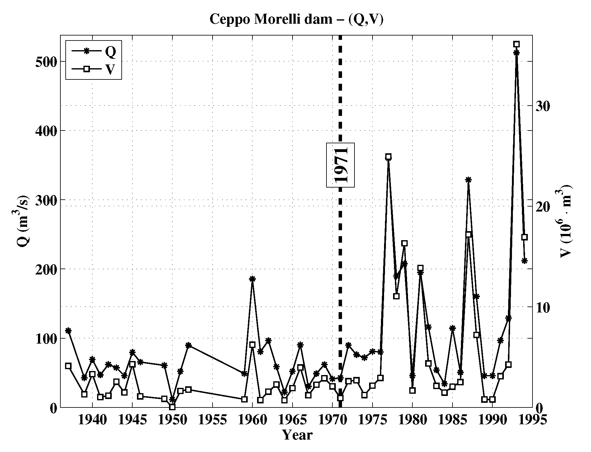
The hydrological data investigated in the following are collected at the Ceppo Morelli dam (Northern Italy), and are the same ones considered in [10,11,12,13], to which the reader is referred. Maximum annual flood peaks Q and volumes V are identified and selected for 49 years, from 1937 to 1994 (some years are missing—see Figure 1). In turn, the case study used to illustrate the general-purpose methodology outlined in this paper—which can be adopted for investigating any environmental hazard—concerns flood hazards involving the traditional variables peak and volume.
Interestingly enough, this database represents an exceptional case study as compared to traditional hydrological ones present in literature: in fact, in hydrological practice, usually the maximum annual flood peak is first selected as a design variable, and then the volume associated with the same flood event is considered, even if it does not represent the annual maximum volume—see, e.g., [14,15]. Instead, in our case, 48 out of 49 of the occurrence dates of the Qs and the Vs are the same (viz., they took place during the same flood episode). In turn, on the one hand, the use of a Block Maxima approach for the Extreme Value analysis is well justified (here, the blocks are the years), and, on the other hand, the “hydrological consistency” of the database is preserved.
3. Methods
A convenient way to deal with multivariate phenomena, where the variables at play are generally non-independent, is to use Copulas [16,17,18]. Since the publication of [19], a number of papers in hydrology, as well as in other environmental areas, have shown the theoretical and practical advantages of using a copula approach, and support its usage. For an overview concerning different ways of quantifying the hazard of compound events, see, among others, [20,21,22,23,24]. In particular, concerning selection/estimation/test statistical procedures for copulas, the interested reader may refer to [25,26,27,28,29,30], and references therein. Note that valuable software for working with copulas, developed for the R package [31], is freely available online [27,32]. The results presented later are obtained using the methodologies outlined in the cited works, to which the reader is referred. In particular, in the following, the same notation used in [11,12,13] is adopted.
Let be the random vector describing the phenomenon under investigation, with univariate marginals s, i.e., . According to Sklar’s Theorem [33], the joint distribution function of can be written as
where is the Copula (viz., the Dependence Structure) of the variables s, assumed to be continuous to ensure the unicity of (as is usually the case in hydrological applications).
As recently discussed in [34], the representation provided by Sklar’s Theorem provides a valuable theoretical tool in order to assess the presence of possible changes of the distributions of hydrological/climate variables (called Change-Points in Statistics)—see also [35,36,37,38] for previous different approaches. In particular, the non-stationarity of may be due to
- changes of any of the marginal distributions s, or
- changes of the copula , or
- both of the previous cases.
In turn, non-parametric Change-Point statistical tests recently outlined in [39,40,41,42] (as well as the corresponding software [43]) can be used to check whether the (multivariate) Null distributional assumption “: has no Change-Points” (viz., does not change with time) should be rejected or not, by investigating whether either the marginals, or the copula, or both, show Change-Points—see, later, Section 4.
Furthermore, let denote the unit interval , and let be the level set of at : practically, is the set of points in the d-dimensional Euclidean space such that —sometimes is also referred to as a “critical layer” of level t [11]. As will be made clear below, plays the role as of a (critical) multivariate threshold, with dimension .
Due to the assumption that the s are strictly increasing—as is the case of the distributions traditionally used in hydrological practice, the Probability Integral Transform (hereinafter, PIT) viz., the relations
and
are one-to-one, where the s are Uniform random variables on . These formulas map the vector living in onto the vector living in the d-dimensional Euclidean space (and vice-versa)—see [16,17,44]. Since copulas are invariant for strictly increasing transformations of the variables at play ([16] Theorem 2.4.3), and share the same copula. Note that the PIT uniquely maps the probabilities of the events in (as induced by the copula ) onto (as induced by ), and vice-versa. The role played by the univariate marginals is only to geometrically re-map such probabilities from onto suitable regions in the Euclidean space (and vice-versa), without affecting them. By the same token, also is uniquely mapped from onto (and vice-versa), thus becoming a level set of .
3.1. Hazard Scenarios
The notion of Hazard Scenario introduced in [13] is fundamental and is briefly recalled below.
Definition 1.
Let model the phenomenon of interest. A Hazard Scenario (hereinafter,HS) of level is any Upper Set such that the following relation holds:
A Hazard Scenario is simply a set containing occurrences s that may damage a structure. By the very definition of Upper Set, if and component-wise, then also could be considered as dangerous, since it “exceeds” .
Given a realization , there exist several ways [13] to associate with a suitable HS . Note that, via Equations (2) and (3), there exists a one-to-one correspondence between and a specific region . In turn, the knowledge of the copula at play may suffice to calculate the level of , and hence of (since they share the same probability).
In general (see, e.g., [13,23]), the choice of the HS should depend upon two criteria: (i) the type of dangerous events, and (ii) their probabilities of occurrence. The approach of interest here is the “OR” one [13], as defined below: in fact, it is sufficient that EITHER Q, OR V, OR both, be large in order to affect/damage the dam (spillway) of interest.
Definition 2.
Given , the associated d-dimensional “OR” Hazard Scenario is given by the region
or, equivalently,
where the function Ψ (introduced in [45]) models and rules the occurrence of dangerous events (viz., when ). The corresponding level α is given by
For the realization of the event it is sufficient that one (or more) of the variables s exceed the corresponding critical threshold (which, usually, is specified by the Regulation, or is inferred by the problem at hand).
3.2. The Failure Probability Approach
A consistent way to assess the hydrological hazard is to compute the corresponding Failure Probability (hereinafter, FP)—for a recent discussion, see [23,24,46]. In this section, the Failure Probability is calculated for the “OR” Hazard Scenario of interest here.
Let be the d-variate vectors describing the phenomenon of interest at times , where is an arbitrary design life time for a given structure: without loss of generality, here T is measured in years. As an example, think of a series of floods s, where and represent, respectively, the annual maximum flood peak and volume observed in the t-th year.
Now, let denote a bivariate critical design threshold (e.g., the one prescribed by the Regulation). Then, each occurrence s can be associated with a precise “OR” HS, given by the region in the plane where either the peak, or the volume, or both exceed the corresponding component of . In turn, a set of “OR” HSs is generated, and each has level given by Equation (7). From a practical point of view, the floods occurring in the complementary regions of the HS’s s could be labelled as “safe”.
In turn, considering the case of independent and identically distributed s, according to Equations (7) and (8), the FP corresponding to the “OR” HS (the one of interest here), for events sharing a common multivariate critical threshold , is given by:
or, equivalently,
In order to provide valuable information for the estimate of, e.g., suitable multivariate design quantiles, further work may be required. In fact, all the infinite realizations lying on the critical layer are associated with the same value of the Failure Probability, since is constant over the level set [13]. This may leave undetermined the assignment of a specific design occurrence, once T and have been chosen. In turn, valuable design values, associated with given Life Times and Failure Probabilities, could be calculated via suitable strategies, e.g., mimicking those outlined in [11,30,49,50,51]. A practical example is given below in Section 4.
4. Results and Discussion
A thorough statistical analysis indicates that Generalized Extreme Value (hereinafter, GEV) marginal distributions adequately fit the observations of both Q and V (see Table 1): this is coherent with the Extreme Value approach adopted, since the variables are annual maxima. The Monte Carlo p-Values of the Kolmogorov–Smirnov Goodness-of-Fit tests are larger than 10%, supporting the validity of the assumed model from a statistical point of view.
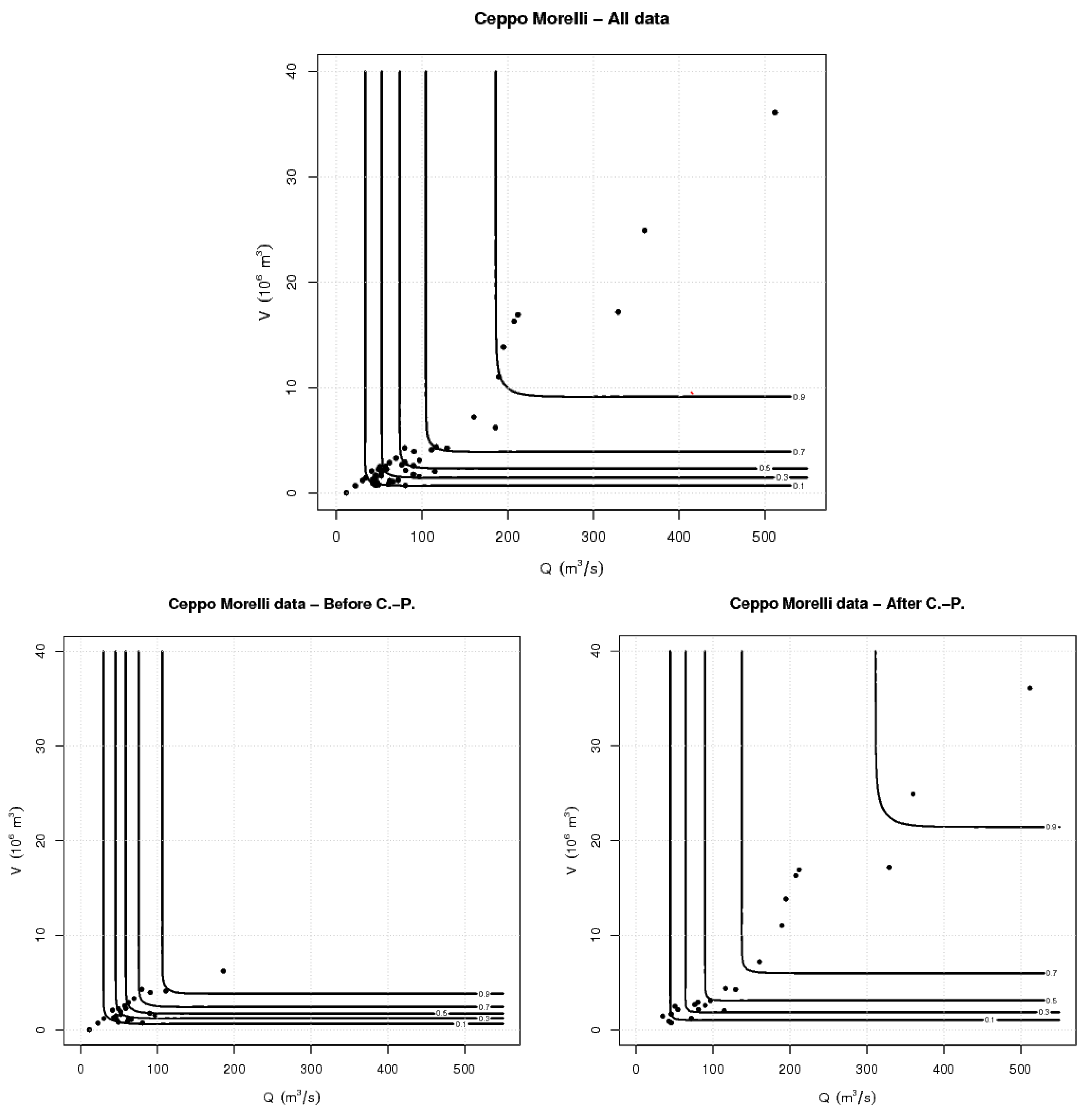
Concerning the bivariate dependence structure of the s, the two variables turn out to be non-independent: in fact, the estimates of the Kendall’s and the Spearman’s are both statistically significantly positive at a 5% level. Here, a survival-Clayton 2-copula is selected among dozens of competing bivariate models, and provides a valuable fit (as indicated by the results of the Goodness-of-Fit (GoF) tests shown in Table 2). Once the marginals and the copula have been fixed, the joint distribution can be computed via Sklar’s Theorem: Figure 2 shows selected isolines of .
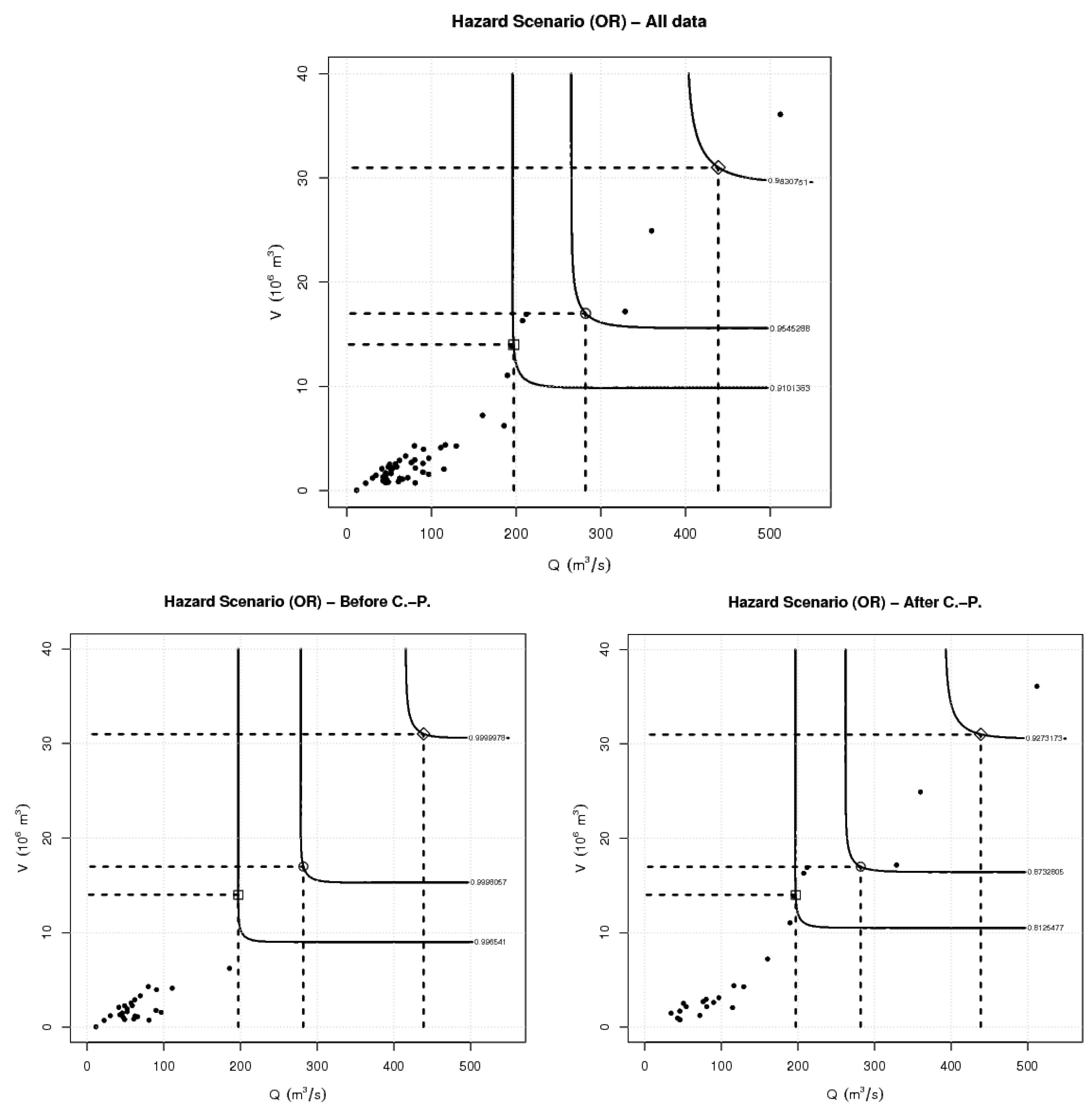
For the sake of illustration, critical bivariate design thresholds s, to be used in Equations (5), (7), and (9) for the calculation of the quantities of interest, are fixed as follows—clearly, other criteria could be adopted, and other values could be chosen. Here, and are assigned the empirical 90%, 95%, and 99% quantiles of, respectively, Q and V (see Table 3). Figure 3 shows the three design pairs s, as well as the corresponding critical layers and the “OR” Hazard Scenarios of interest. The corresponding approximate levels , with , can be calculated via Equation (7), and are reported in Table 3. As expected, (component-wise) “larger” s yield smaller scenario levels s.
As an example, in this work, a life time T, varying from one to 50 years, is chosen. In the first instance, here it is assumed that the occurrences are independent and identically distributed (i.i.d.): while physical and statistical reasons suggest accepting the independence of annual maxima, by contrast the stationarity of their joint distribution might be questionable (e.g., due to a changing climate or human activities), and will be discussed later.
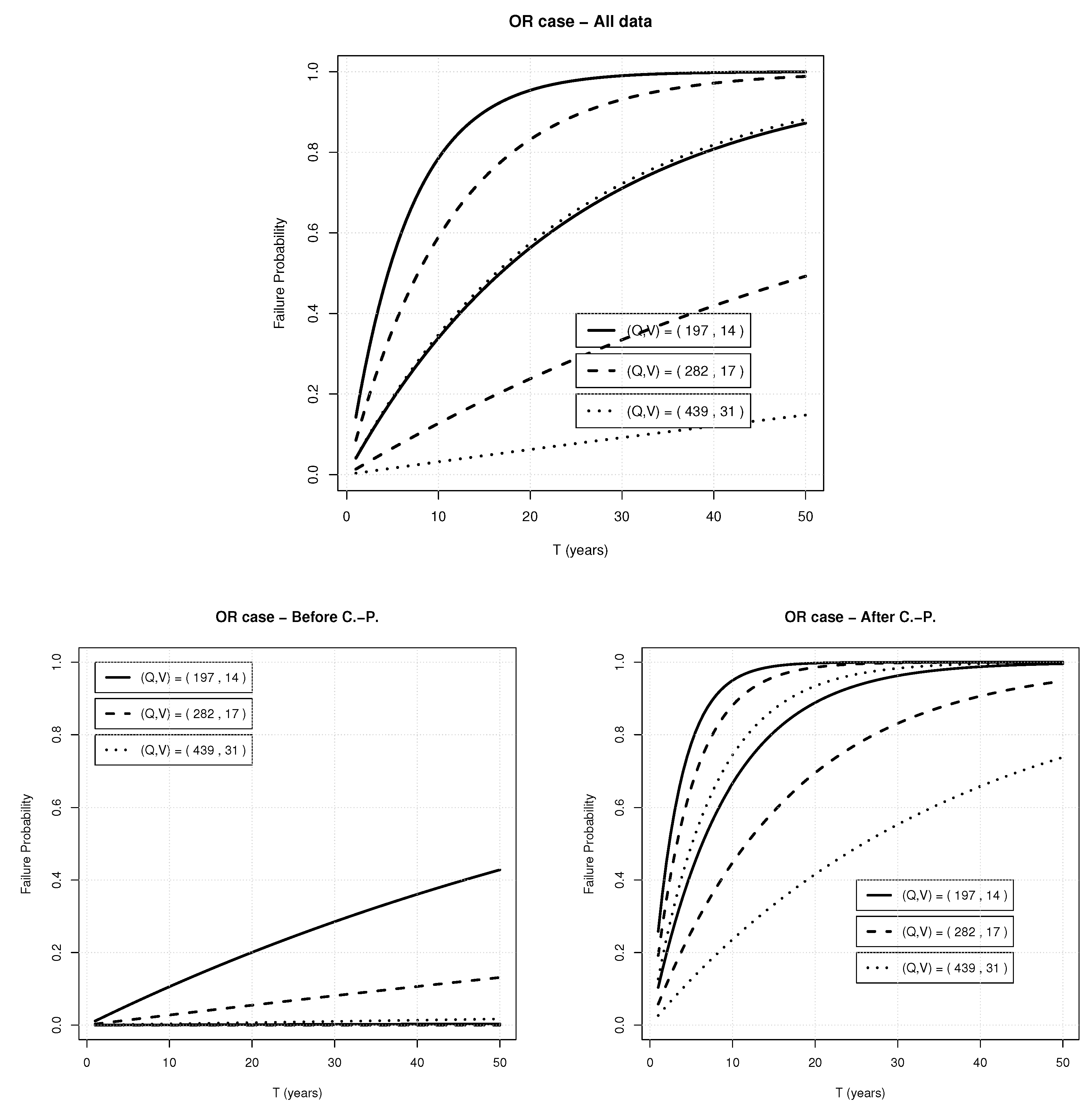
The results under the i.i.d. assumption are shown in Figure 4(top): here, Monte Carlo Confidence Bands (at a 90% level) for the Failure Probabilities s associated with the design pairs s are plotted. In all cases, the width of the bands is very large: the explanation is as follows. The shape parameters of the fitted GEV marginals are close to (or larger than) 1/2—see Table 1: interestingly enough, the parameters have also been estimated via the L-moments method, yielding comparable results (not shown). In turn, the existence of the second order moments (i.e., the variances) may be questionable, and large fluctuations during the simulations have to be expected, which may adversely affect the Monte Carlo procedure and yield very wide bands. Unfortunately, situations like these are common in hydrological practice, but little can be done to reduce the uncertainties shown in the plots: it is a problem intrinsic to the very structure of the available data.
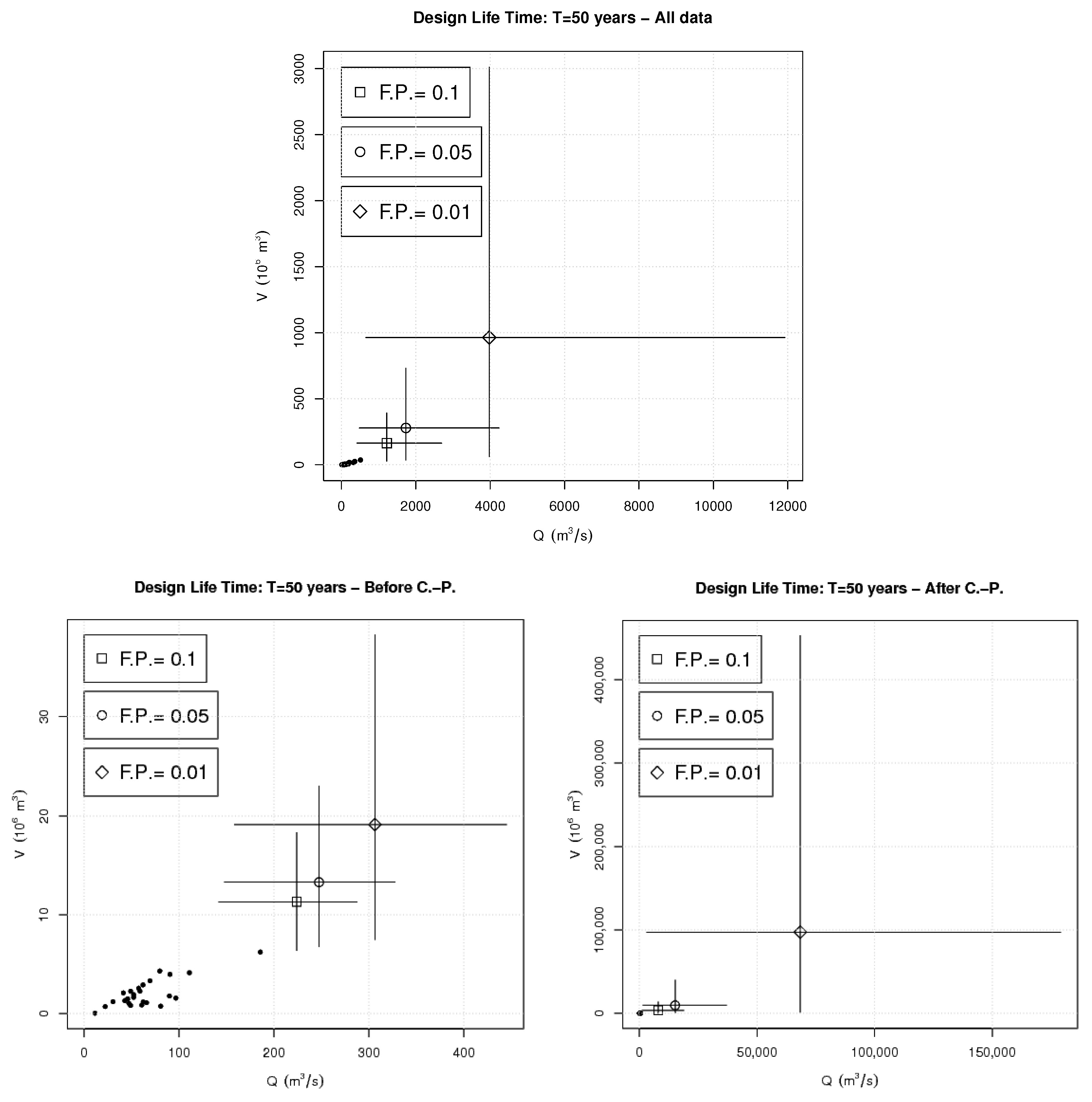
Concerning the computation of suitable multivariate design quantiles, here a Most Likely strategy is used [11,30]. Practically, the level set associated with selected values of T and is considered, and the occurrence which maximizes the density over , is taken as a design pair. Figure 5(top) shows the design pairs corresponding to a lifetime years and Failure Probabilities of order, respectively, 10%, 5%, and 1%, as well as Monte Carlo Confidence Intervals at a 90% level: as already discussed above, large unavoidable uncertainties are present.
As a second instance, it may be of interest to study how the previous results might be affected by a change of the joint distribution of the phenomenon under investigation (for a similar hydrological case study see, e.g., [9,52]). Specifically, a distributional change of the behavior of the pair may be due to:
- a change of the univariate distribution (respectively, ), or
- a change of the copula associated with , or
- both the previous instances.
Here, possible changes are detected according to different tests recently introduced in literature—see [39,40,41,42], and implemented in the R package npcp [43].
In the present case, apparently, the overall stochastic behavior shown in Figure 1 might have changed around the year 1971: see below, and Table 1 and Table 2. More precisely, according to the approximate p-Value of the test (about 4%), the Null hypothesis that the joint distribution has not changed could not be rejected at the standard 1% level, but should be rejected at the 5% and 10% ones. Actually, might also have changed around 1971 (the p-Value is about 3%), as well as around 1970 (the p-Value is about 2.5%), and around 1975 (the p-Value is about 2.8%). In turn, given the intrinsic uncertainties of the test [39], the critical year associated with the Change-Point is reasonably and practically assumed to be 1971 (also considering that, in hydrology, Q is traditionally indicated as the regulation variable). Apparently, this is consistent with the claims of [53], stating that “… the 1970s are known as a period of major climate and environmental changes observed in several proxies and several fields at the global scale, as attested to in many recent studies [54,55,56,57,58,59].”
Whether or not the dynamics of the phenomenon has really changed (concerning this latter issue, instructive is the recent work by [4]), it is however interesting to study the possible effects on the strategies of hazard assessment, e.g., in terms of the Failure Probabilities discussed in this work. For this purpose, both the marginals and the copula of the subsets of observations before and after 1971 were computed: the results are reported in Table 1 and Table 2, and illustrated in Figure 2 and Figure 6. In turn, both the GEV univariate laws and the survival-Clayton 2-copula still provide valuable models for these data sets, but the corresponding parameters have changed. More specifically, the observations can be fitted by distributions and copulas showing two distinct regimes (before and after 1971), and modeled by the same univariate and bivariate functions with different parameters. Note that no further Change-Points are detected in each of the two sub-periods before and after 1971.
The behavior of the FPs, assuming that the joint probability distribution has changed in 1971, is plotted in Figure 4(bottom): in general, the failure probabilities assuming stationarity are smaller than the ones after 1971, while the uncertainties are again large. Apparently, there is a remodeling of the dynamics of the temporal series of floods: actually, both univariate and multivariate parameters change. In particular, an increase of the statistical dependence between flood peak and flood volume may be likely. These results may indicate an intensification of the flood events in the period 1971–1994, both in the dependence structure and in the marginals, and consequently an increase of the corresponding failure probabilities. Similar conclusions can be drawn concerning the computation of suitable design pairs, as shown in Figure 5(bottom): again, for the same reasons mentioned above, large uncertainties are present.
5. Conclusions
The possible presence of a distributional Change-Point in a hydrologic bivariate dataset of maximum annual flood peaks and volumes has been investigated, in order to evaluate the consequences of possible violations of the stationarity assumption from a hazard assessment perspective. In particular, the assessment of the environmental hazard has been carried via the theory of Copulas and the Failure Probabilities. The impact is evaluated adopting a risk-manager perspective.
The investigation carried out in this work makes it evident that it may be important to test the stationarity assumption, viz. to check whether (or not) the stochastic behavior of the variables at play might have changed with time, in terms of a change of the families of marginal probability distributions, and/or a change of the associated copula family, and/or a change of the corresponding parameters’ values.
Apparently, considering the case study investigated here, the statistical analyses indicate that a distributional Change-Point might be present around 1971: actually, the estimates of the parameters of both the marginals and the copula are different in a time period before and after 1971 (whereas the families of the distributions might not have changed). In turn, a due analysis (in terms of Failure Probabilities) of the effects of the possible presence of a Change-Points on the hazard assessment has been carried out.
As a conclusion, under the assumption that the hydrological regime has really changed, the corresponding increase of the FPs yields a strengthening of the estimated threatening: clearly, neglecting such a dynamics might provide an unrealistic hazard assessment. However, such a diagnosis is essentially of a statistical nature: in our opinion, further physical considerations are needed in order to correctly guide the decisions of the Water Managers, which only a proper and correct engineering practice may provide. In our opinion, further analyses are needed in order to understand whether a similar behavior is present also in other neighboring sites, and to check whether analogous conclusions could be drawn also for, e.g., precipitation, droughts, etc. (see, e.g., the scenarios’ procedures outlined in [60,61], as well as [62] for recent multivariate characterizations). Actually, combined together, such pieces of information could provide valuable evidence concerning possible climate changes, and supply indications about plausible future hydrologic scenarios. Finally, the presence of heavy tailed marginals (a common situation in hydrological time series) further complicates the analyses by introducing additional uncertainties, as discussed in the paper.
As a general recommendation, it is important to stress that the statistical outcomes should always be “validated/supported/confirmed” via additional practical investigations, such as a regional analysis of other relevant hydrological variables like discharge, precipitation, etc. In terms of flood hazard management, the results presented here suggest that, for checking the adequacy and the functionality of existing water works, a statistical (multivariate) survey represents a necessary step, though it may not be sufficient.
Author Contributions
Data curation, C.D.M.; Formal analysis, G.S., F.D., C.D.M. and M.B.; Methodology, G.S., F.D. and M.B. The R software packages copula and npcp (cited in the manuscript) have been used to carry out the investigations. All authors analysed the results and reviewed the manuscript.
Acknowledgments
Helpful discussions with Christian Genest (McGill University, Montréal, Québec, Canada), Ivan Kojadinovic (Université de Pau et des Pays de l’Adour, Pau, France), and Carlo Sempi (Università del Salento, Lecce, Italy) are acknowledged. (GS) The support of the CMCC (Centro Euro-Mediterraneo sui Cambiamenti Climatici, Lecce (Italy)) is acknowledged.
Conflicts of Interest
The authors declare no conflicts of interest.
References
- Kantz, H.; Schreiber, T. Nonlinear Time Series Analysis, 2nd ed.; Cambridge University Press: Cambridge, UK, 2008. [Google Scholar]
- Bendat, J.; Piersol, A. Random Data: Analysis and Measurement Procedures, 4st ed.; John Wiley & Sons Inc.: Hoboken, NJ, USA, 2010. [Google Scholar]
- Rao, A.; Hamed, K.; Chen, H.L. Nonstationarities in Hydrologic and Environmental Time Series, 1st ed.; Kluwer Academic Publishers: Dordrecht, The Netherlands, 2003. [Google Scholar]
- Montanari, A.; Koutsoyiannis, D. Modeling and mitigating natural hazards: Stationarity is immortal! Water Resour. Res. 2014, 50, 9748–9756. [Google Scholar] [CrossRef] [Green Version]
- Koutsoyiannis, D.; Montanari, A. Negligent killing of scientific concepts: The stationarity case. Hydrol. Sci. J. 2015, 60, 1174–1183. [Google Scholar] [CrossRef]
- Milly, P.; Betancourt, J.; Falkenmark, M.; Hirsch, R.; Kundzewicz, Z.; Lettenmaier, D.; Stouffer, R. Climate change—Stationarity is dead: Whither water management? Science 2008, 319, 573–574. [Google Scholar] [CrossRef] [PubMed]
- Kundzewicz, Z.; Robson, A. Detecting Trend and Other Changes in Hydrological Data. Water, World Climate Programme Data and Monitoring; Volume WMO/TD—No. 1013; World Meteorological Organization: Geneva, Switzerland, 2000. [Google Scholar]
- Kundzewicz, Z.; Robson, A. Change detection in hydrological records—A review of the methodology. Hydrol. Sci. J. 2004, 49, 7–19. [Google Scholar] [CrossRef]
- Ben Aissia, M.A.; Chebana, F.; Ouarda, T.; Roy, L.; Bruneau, P.; Barbet, M. Dependence evolution of hydrological characteristics, applied to floods in a climate change context in Quebec. J. Hydrol. 2014, 519, 148–163. [Google Scholar] [CrossRef]
- De Michele, C.; Salvadori, G.; Canossi, M.; Petaccia, A.; Rosso, R. Bivariate statistical approach to check adequacy of dam spillway. ASCE J. Hydrol. Eng. 2005, 10, 50–57. [Google Scholar] [CrossRef]
- Salvadori, G.; De Michele, C.; Durante, F. On the return period and design in a multivariate framework. Hydrol. Earth Syst. Sci. 2011, 15, 3293–3305. [Google Scholar] [CrossRef] [Green Version]
- Salvadori, G.; Durante, F.; De Michele, C. Multivariate return period calculation via survival functions. Water Resour. Res. 2013, 49, 2308–2311. [Google Scholar] [CrossRef] [Green Version]
- Salvadori, G.; Durante, F.; De Michele, C.; Bernardi, M.; Petrella, L. A multivariate Copula-based framework for dealing with Hazard Scenarios and Failure Probabilities. Water Resour. Res. 2016, 52, 3701–3721. [Google Scholar] [CrossRef]
- Mediero, L.; Jimenez-Alvarez, A.; Garrote, L. Design flood hydrographs from the relationship between flood peak and volume. Hydrol. Earth Syst. Sci. 2010, 14, 2495–2505. [Google Scholar] [CrossRef] [Green Version]
- Gaál, L.; Szolgay, J.; Kohnová, S.; Hlavčová, K.; Parajka, J.; Viglione, A.; Merz, R.; Blöschl, G. Dependence between flood peaks and volumes: A case study on climate and hydrological controls. Hydrol. Sci. J. 2015, 60, 968–984. [Google Scholar] [CrossRef]
- Nelsen, R. An Introduction to Copulas, 2nd ed.; Springer: New York, NY, USA, 2006. [Google Scholar]
- Salvadori, G.; De Michele, C.; Kottegoda, N.; Rosso, R. Extremes in Nature. An Approach Using Copulas; Water Science and Technology Library; Springer: Dordrecht, The Netherlands, 2007; Volume 56. [Google Scholar]
- Durante, F.; Sempi, C. Principles of Copula Theory; CRC/Chapman & Hall: Boca Raton, FL, USA, 2016. [Google Scholar]
- De Michele, C.; Salvadori, G. A Generalized Pareto intensity-duration model of storm rainfall exploiting 2-Copulas. J. Geophys. Res. 2003, 108, 4067. [Google Scholar] [CrossRef]
- Gräler, B.; van den Berg, M.J.; Vandenberghe, S.; Petroselli, A.; Grimaldi, S.; Baets, B.D.; Verhoest, N.E.C. Multivariate return periods in hydrology: A critical and practical review focusing on synthetic design hydrograph estimation. Hydrol. Earth Syst. Sci. 2013, 17, 1281–1296. [Google Scholar] [CrossRef] [Green Version]
- Dutfoy, A.; Parey, S.; Roche, N. Multivariate Extreme Value Theory—A Tutorial with Applications to Hydrology and Meteorology. Depend. Model. 2014, 2. [Google Scholar] [CrossRef]
- Salas, J.; Obeysekera, J. Revisiting the Concepts of Return Period and Risk for Nonstationary Hydrologic Extreme Events. J. Hydrol. Eng. 2014, 19, 554–568. [Google Scholar] [CrossRef]
- Serinaldi, F. Dismissing return periods! Stoch. Environ. Res. Risk Assess. 2015, 29, 1179–1189. [Google Scholar] [CrossRef]
- Moftakhari, H.R.; Salvadori, G.; AghaKouchak, A.; Sanders, B.F.; Matthew, R.A. Compounding effects of sea level rise and fluvial flooding. Proc. Natl. Acad. Sci. USA 2017, 114, 9785–9790. [Google Scholar] [CrossRef] [PubMed] [Green Version]
- Genest, C.; Favre, A. Everything you always wanted to know about copula modeling but were afraid to ask. J. Hydrol. Eng. 2007, 12, 347–368. [Google Scholar] [CrossRef]
- Genest, C.; Rémillard, B.; Beaudoin, D. Goodness-of-fit tests for copulas: A review and a power study. Insur. Math. Econ. 2009, 44, 199–213. [Google Scholar] [CrossRef]
- Kojadinovic, I.; Yan, J. Modeling multivariate distributions with continuous margins using the copula R package. J. Stat. Softw. 2010, 34, 1–20. [Google Scholar] [CrossRef]
- Kojadinovic, I.; Yan, J.; Holmes, M. Fast large-sample goodness-of-fit tests for copulas. Stat. Sin. 2011, 21, 841–871. [Google Scholar] [CrossRef]
- Joe, H. Dependence Modeling with Copulas; Chapman & Hall/CRC: London, UK, 2014. [Google Scholar]
- Salvadori, G.; Tomasicchio, G.R.; D’Alessandro, F. Practical guidelines for multivariate analysis and design in coastal and off-shore engineering. Coast. Eng. 2014, 88, 1–14. [Google Scholar] [CrossRef]
- R Core Team. R: A Language and Environment for Statistical Computing; R Foundation for Statistical Computing: Vienna, Austria, 2016. [Google Scholar]
- Hofert, M.; Kojadinovic, I.; Maechler, M.; Yan, J. Copula: Multivariate Dependence with Copulas; R Package Version 0.999-17; R Package: Vienna, Austria, 2017. [Google Scholar]
- Sklar, A. Fonctions de répartition à n dimensions et leurs marges. Publ. Inst. Stat. Univ. Paris 1959, 8, 229–231. [Google Scholar]
- Vezzoli, R.; Salvadori, G.; De Michele, C. A distributional multivariate approach for assessing performance of climate-hydrology models. Nat. Sci. Rep. 2017, 7, 12071. [Google Scholar] [CrossRef] [PubMed] [Green Version]
- Chebana, F.; Ouarda, T.B.; Duong, T.C. Testing for multivariate trends in hydrologic frequency analysis. J. Hydrol. 2013, 486, 519–530. [Google Scholar] [CrossRef]
- Volpi, E.; Fiori, A.; Grimaldi, S.; Lombardo, F.; Koutsoyiannis, D. One hundred years of return period: Strengths and limitations. Water Resour. Res. 2015, 51, 8570–8585. [Google Scholar] [CrossRef]
- Xiong, L.; Jiang, C.; Xu, C.Y.; Yu, K.X.; Guo, S. A framework of change-point detection for multivariate hydrological series. Water Resour. Res. 2015, 51, 8198–8217. [Google Scholar] [CrossRef]
- Ye, L.; Zhou, J.; Zeng, X.; Tayyab, M. Hydrological Mann-Kendal Multivariate Trends Analysis in the Upper Yangtze River Basin. J. Geosci. Environ. Prot. 2015, 3, 34–39. [Google Scholar] [CrossRef]
- Holmes, M.; Kojadinovic, I.; Quessy, J.F. Nonparametric tests for change-point detection à la Gombay and Horváth. J. Multivar. Anal. 2013, 115, 16–32. [Google Scholar] [CrossRef]
- Bücher, A.; Kojadinovic, I.; Rohmer, T.; Segers, J. Detecting changes in cross-sectional dependence in multivariate time series. J. Multivar. Anal. 2014, 132, 111–128. [Google Scholar] [CrossRef] [Green Version]
- Bücher, A.; Kojadinovic, I. A dependent multiplier bootstrap for the sequential empirical copula process under strong mixing. Bernoulli 2016, 22, 927–968. [Google Scholar] [CrossRef] [Green Version]
- Kojadinovic, I.; Naveau, P. Nonparametric tests for change-point detection in the distribution of block maxima based on probability weighted moments. Extremes 2017, 20, 417–450. [Google Scholar] [CrossRef]
- Kojadinovic, I. npcp: Some Nonparametric CUSUM Tests for Change-Point Detection in Possibly Multivariate Observations; R Package Version 0.1-9.; R Package: Vienna, Austria, 2017. [Google Scholar]
- Embrechts, P.; Hofert, M. A note on generalized inverses. Math. Methods Oper. Res. 2013, 77, 423–432. [Google Scholar] [CrossRef] [Green Version]
- Bernardi, M.; Durante, F.; Jaworski, P.; Petrella, L.; Salvadori, G. Conditional risk based on multivariate hazard scenarios. Stoch. Environ. Res. Risk Assess. 2018, 32, 203–211. [Google Scholar] [CrossRef]
- Read, L.K.; Vogel, R.M. Reliability, return periods, and risk under nonstationarity. Water Resour. Res. 2015, 51, 6381–6398. [Google Scholar] [CrossRef] [Green Version]
- Chow, V.T.; Maidment, D.; Mays, L.W. Applied Hydrology, 1st ed.; McGraw-Hill: Singapore, 1988. [Google Scholar]
- Kottegoda, N.; Rosso, R. Applied Statistics for Civil and Environmental Engineers; Wiley-Blackwell: Oxford, UK, 2008. [Google Scholar]
- Chebana, F.; Ouarda, T.B.M.J. Multivariate quantiles in hydrological frequency analysis. Environmetrics 2011, 22, 63–78. [Google Scholar] [CrossRef] [Green Version]
- Corbella, S.; Stretch, D.D. Multivariate return periods of sea storms for coastal erosion risk assessment. Nat. Hazards Earth Syst. Sci. 2012, 12, 2699–2708. [Google Scholar] [CrossRef]
- AghaKouchak, A.; Cheng, L.; Mazdiyasni, O.; Farahmand, A. Global warming and changes in risk of concurrent climate extremes: Insights from the 2014 California drought. Geophys. Res. Lett. 2014, 41, 8847–8852. [Google Scholar] [CrossRef] [Green Version]
- Ben Aissia, M.A.; Chebana, F.; Ouarda, T.; Roy, L.; Desrochers, G.; Chartier, I.; Robichaud, É. Multivariate analysis of flood characteristics in a climate change context of the watershed of the Baskatong reservoir, Province of Québec, Canada. Hydrol. Process 2012, 26, 130–142. [Google Scholar] [CrossRef]
- Massei, N.; Laignel, B.; Deloffre, J.; Mesquita, J.; Motelay, A.; Lafite, R.; Durand, A. Long-term hydrological changes of the Seine River flow (France) and their relation to the North Atlantic Oscillation over the period 1950–2008. Int. J. Climatol. 2010, 30, 2146–2154. [Google Scholar] [CrossRef]
- Alexander, M.; Capotondi, A.; Miller, A.; Chai, F.; Brodeur, R.; Deser, C. Decadal variability in the northeast Pacific in a physical-ecosystem model: Role of mixed layer depth and trophic interactions. J. Geophys. Res. Oceans 2008, 113. [Google Scholar] [CrossRef] [Green Version]
- Alheit, J.; Niquen, M. Regime shifts in the Humboldt Current ecosystem. Prog. Oceanogr. 2004, 60, 201–222. [Google Scholar] [CrossRef]
- Daskalov, G. Long-term changes in fish abundance and environmental indices in the Black Sea. Mar. Ecol. Prog. Ser. 2003, 255, 259–270. [Google Scholar] [CrossRef] [Green Version]
- Dickson, B.; Osterhus, S. One hundred years in the Norwegian Sea. Norsk Geogr. Tidsskr. Nor. J. Geogr. 2007, 61, 56–75. [Google Scholar] [CrossRef] [Green Version]
- Schwing, F.; Murphree, T.; Green, P. The Northern Oscillation index (NOI): A new climate index for the northeast Pacific. Prog. Oceanogr. 2002, 53, 115–139. [Google Scholar] [CrossRef]
- Serreze, M.; Walsh, J.; Chapin, F.; Osterkamp, T.; Dyurgerov, M.; Romanovsky, V.; Oechel, W.; Morison, J.; Zhang, T.; Barry, R. Observational evidence of recent change in the northern high-latitude environment. Clim. Chang. 2000, 46, 159–207. [Google Scholar] [CrossRef]
- De Michele, C.; Salvadori, G.; Vezzoli, R.; Pecora, S. Multivariate assessment of droughts: Frequency analysis and Dynamic Return Period. Water Resour. Res. 2013, 49, 6985–6994. [Google Scholar] [CrossRef]
- Salvadori, G.; De Michele, C. Multivariate real-time assessment of droughts via Copula-based multi-site Hazard Trajectories and Fans. J. Hydrol. 2014. [Google Scholar] [CrossRef]
- Hao, Z.; AghaKouchak, A. Multivariate Standardized Drought Index: A parametric multi-index model. Adv. Water Resour. 2013, 57, 12–18. [Google Scholar] [CrossRef]
Figure 1.
Time series of the available Q and V data—see text. The vertical dashed line indicates the possible Change-Point year (1971).
Figure 1.
Time series of the available Q and V data—see text. The vertical dashed line indicates the possible Change-Point year (1971).

Figure 2.
Observed pairs s (markers), and selected isolines of the fitted distribution —see text: (Top panel) all data; (Bottom-left panel) the data before the Change-Point year; (Bottom-right panel) the data after the Change-Point year.
Figure 2.
Observed pairs s (markers), and selected isolines of the fitted distribution —see text: (Top panel) all data; (Bottom-left panel) the data before the Change-Point year; (Bottom-right panel) the data after the Change-Point year.

Figure 3.
Observed pairs s (full circles), “OR” Hazard Scenarios (the regions “above” the dashed lines), the design pairs indicated in Table 3 (respectively, empty square, circle, and diamond), and isolines of the fitted crossing the design pairs—see text: (Top panel) all data; (Bottom-left panel) the data before the Change-Point year; (Bottom-right panel) the data after the Change-Point year.

Figure 4.
Confidence bands (at a 90% level) for the Failure Probabilities s associated with the design pairs s plotted in Figure 3—see text: (Top panel) all data; (Bottom-left panel) before the Change-Point year; (Bottom-right panel) after the Change-Point year.
Figure 4.
Confidence bands (at a 90% level) for the Failure Probabilities s associated with the design pairs s plotted in Figure 3—see text: (Top panel) all data; (Bottom-left panel) before the Change-Point year; (Bottom-right panel) after the Change-Point year.

Figure 5.
Observed pairs s (full circles), and mean “Most Likely” design pairs s (markers) for different design Failure Probabilities—see text: (Top panel) all data; (Bottom-left panel) before the Change-Point year; (Bottom-right panel) after the Change-Point year. Also shown are Monte Carlo Confidence Intervals at a 90% level.

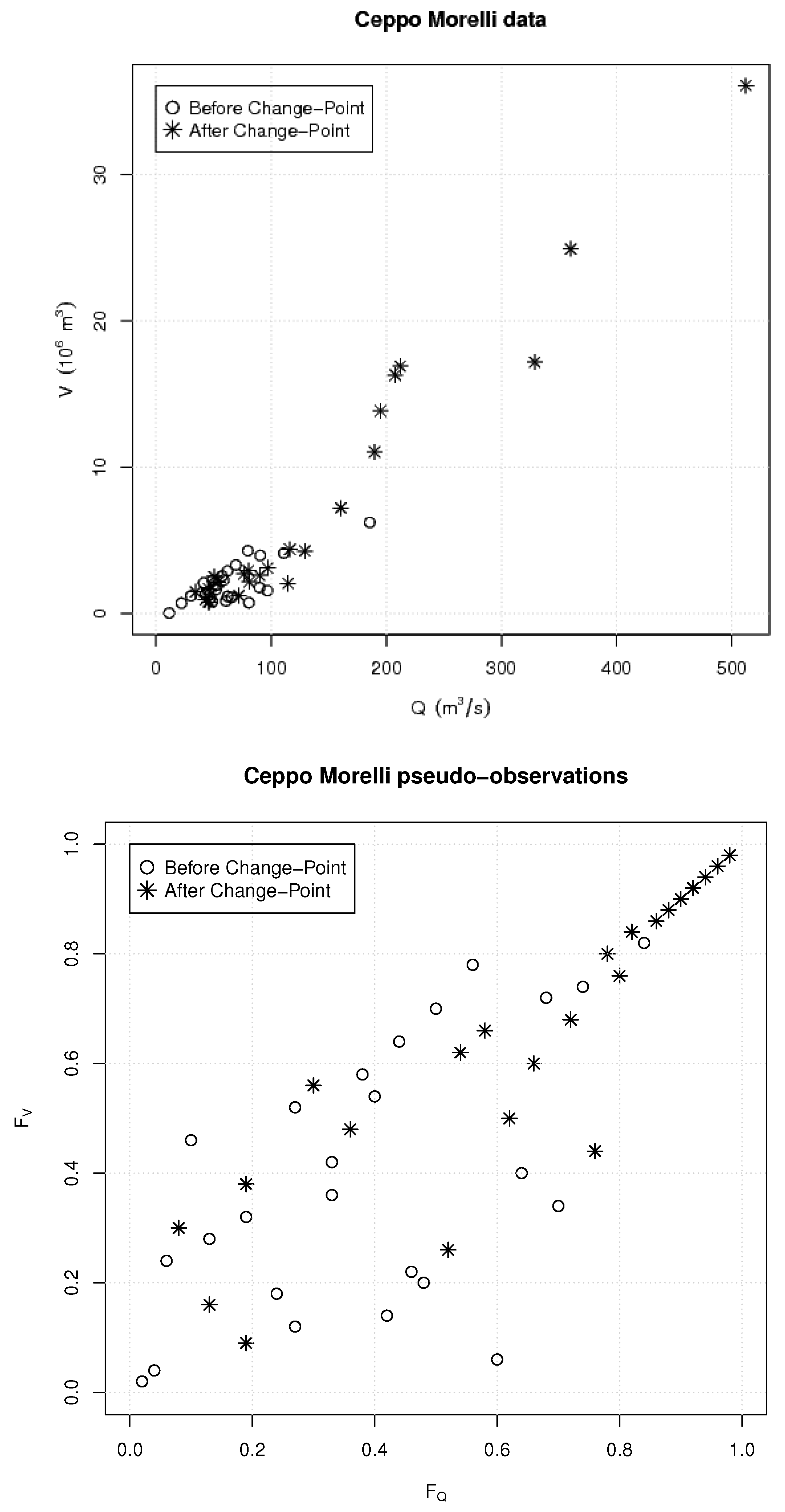
Figure 6.
The available observations—see text: (Top panel) the data; (Bottom panel) the pseudo-observations, viz. the normalized ranks. The occurrences before and after the possible Change-Point year are indicated via different markers.
Figure 6.
The available observations—see text: (Top panel) the data; (Bottom panel) the pseudo-observations, viz. the normalized ranks. The occurrences before and after the possible Change-Point year are indicated via different markers.


Table 1.
Maximum Likelihood estimates of the parameters of the GEV distributions fitting the variables Q (in m/s) and V (in 10 m), either considering all the data, or only those collected, respectively, before and after the Change-Point year (1971)—see text. Also shown are estimated standard errors and approximate Monte Carlo Goodness-of-Fit test p-Values (based on Kolmogorov–Smirnov statistics).
| Variable | Shape | Scale | Position | p-Value |
|---|---|---|---|---|
| All data | ||||
| Q | 0.37 | 36.21 | 59.36 | 77% |
| s.e. | 0.11 | 5.04 | 5.71 | |
| V | 0.61 | 1.52 | 1.72 | 91% |
| s.e. | 0.13 | 0.25 | 0.24 | |
| Before Change-Point | ||||
| Q | 0.02 | 24.46 | 50.05 | 87% |
| s.e. | 0.11 | 3.79 | 5.36 | |
| V | 0.12 | 0.95 | 1.39 | 99% |
| s.e. | 0.16 | 0.16 | 0.21 | |
| After Change-Point | ||||
| Q | 0.71 | 42.96 | 71.74 | 98% |
| s.e. | 0.30 | 11.75 | 10.92 | |
| V | 1.07 | 2.03 | 2.20 | 92% |
| s.e. | 0.34 | 0.67 | 0.50 | |
Table 2.
Maximum Likelihood estimates of the survival-Clayton 2-copula parameter fitting the pairs s, either considering all the data, or only those collected, respectively, before and after the Change-Point year (1971)—see text. Also shown are estimated standard errors and approximate p-Values (via a Multiplier Method) of the Cramér–von Mises Goodness-of-Fit test for Copulas based on the copula empirical process [32].
| All Data | Before Change-Point | After Change-Point | |
|---|---|---|---|
| 4.33 | 1.53 | 11.69 | |
| s.e. | 1.37 | 0.72 | 5.31 |
| p-Value | 9% | 47% | 44% |
Table 3.
The design pairs s—see text: the units are m/s for Q, and 10m for V. Also shown are the corresponding estimates of the “OR” HS levels s.
Table 3.
The design pairs s—see text: the units are m/s for Q, and 10m for V. Also shown are the corresponding estimates of the “OR” HS levels s.
| Quantile (%) | Q | V | ||
|---|---|---|---|---|
| 90% | 197 | 14 | 0.0880 | |
| 95% | 282 | 17 | 0.0453 | |
| 99% | 439 | 31 | 0.0172 |
© 2018 by the authors. Licensee MDPI, Basel, Switzerland. This article is an open access article distributed under the terms and conditions of the Creative Commons Attribution (CC BY) license (http://creativecommons.org/licenses/by/4.0/).
Share and Cite
MDPI and ACS Style
Salvadori, G.; Durante, F.; De Michele, C.; Bernardi, M. Hazard Assessment under Multivariate Distributional Change-Points: Guidelines and a Flood Case Study. Water 2018, 10, 751. https://doi.org/10.3390/w10060751
AMA Style
Salvadori G, Durante F, De Michele C, Bernardi M. Hazard Assessment under Multivariate Distributional Change-Points: Guidelines and a Flood Case Study. Water. 2018; 10(6):751. https://doi.org/10.3390/w10060751
Chicago/Turabian StyleSalvadori, Gianfausto, Fabrizio Durante, Carlo De Michele, and Mauro Bernardi. 2018. "Hazard Assessment under Multivariate Distributional Change-Points: Guidelines and a Flood Case Study" Water 10, no. 6: 751. https://doi.org/10.3390/w10060751
Note that from the first issue of 2016, this journal uses article numbers instead of page numbers. See further details here.