Influence of Climate Change on the Design of Retention Basins in Northeastern Portugal

Abstract

Retention basins are used to control the quantity and quality of stormwater runoff. Their design is based on Intensity-Duration-Frequency (IDF) curves and on the assumption that the rainfall distribution is stationary. The analysis of rainfall observed for recent past conditions and projected for the future suggests the existence of significant changes in the frequency and intensity of extreme rainfall events. This study aims to assess the potential impacts of climate change in the design of retention basins. The adopted multi- and interdisciplinary methodological approach comprises: Rainfall aggregation and disaggregation, distribution fitting for different climate change scenarios, durations and return periods, model bias correction, robust regression of rainfall intensity for different durations and, finally, engineering design based on IDF curves. Results obtained with IDF curves defined in the Portuguese law and estimated from the ECHAM5/MPI-OM1/COSMO-CLM regional climate model for recent past and future climate scenarios point to: (i) Increase in the volume of the retention basin, more expressive in the end of the XXI century; (ii) changes of different magnitude within the country and the same rainfall region; and (iii) increase of 20% to 23% on average, and 46% to 65% at most, for the conditions of B1 and A1B scenarios, respectively.

1. Introduction

Retention or detention basins are surface storage basins or facilities intended to attenuate and manage storm water runoff and control flooding by dampening the peak flows through temporary storage [1,2]. The main objectives of these waterworks are the protection of the environment by controlling water pollution by trapping and removing nutrients, metals, and pathogens and control ecotoxicity from urban and industrial catchments runoff, prevent downstream erosion, creating alternative water reserves for firefighting, irrigation and minimize droughts as well as creating water mirrors with recreational and aesthetic interest among many others [3,4,5,6]. Numerous studies have been performed to improve environmental and economic efficiency of these waterworks (e.g., [7,8,9,10,11,12,13,14,15]).

The design of storm water runoff drainage systems is mainly based on the relationship of Intensity-Duration-Frequency (hereafter, IDF) curves [16,17,18], which, in Portugal, are defined by law [19]. The use of these curves relied on the assumption that the statistical distribution of intense rainfall is statistically stationary, i.e., the statistical distribution is not changing over time, in quantity or condition. However, evidences of changes in the rainfall regime have been noticed all over the globe in recent past and projected for future conditions, especially in terms of the frequency and intensity of extreme events, suggesting the need to review, update and adapt the design of drainage systems for climate change [20,21,22,23,24].

Global Circulation Models (GCM) are the cornerstone tools to study climate change [25]. However, their spatial resolution, ranging from tens to hundreds of kilometers, is extremely high to capture small scale phenomena so that their simulations can be used at a local scale [26]. Furthermore, simulations of GCM are usually only available at daily scale, which are inadequate to study urban flooding that tends to occur with high rainfall intensity for shorter durations [27]. Projections of climate change with higher spatial-temporal resolution may be derived from different regionalization techniques [28], comprising high- and variable-resolution GCMs [29,30], statistical downscaling [31] and nested Regional Climate Models (RCM) [32]. A comprehensive review of downscaling methods and applications are available in the literature, including for hydrological modelling (e.g., [25,33,34]). Dynamical downscaling with RCMs is the best downscaling solution because their much higher resolution spatial grids can take into account the specific characteristics of the study area such as complex topography, land use/land cover inhomogeneities and land-sea distribution [35] as well as to simulate the sub-daily/hourly temporal evolution of the meteorological variables more accurately. Advantages and limitations of RCM to downscale climate change and their skill to forecast rainfall are comprehensively reviewed in [26]. RCMs forced by GCMs have been used in recent years to physically downscale GCM’s rainfall projections for different future climate scenarios for Portugal (e.g., [23,36,37]).

The typical sampling periods of observation networks and RCMs temporal resolution are usually too high to be directly used to estimate IDF curves. Consequently, it is often necessary to disaggregate the rainfall data to hourly and sub-hourly temporal scales. Available methodologies involve simulations of rainfall in sub-hourly duration in association with simulated series from stochastic models of disaggregation (e.g., [38,39]). For example, the software HYETOS R [40] was recently used to disaggregate rainfall in many regions and for different purposes [41,42,43]. However, the method of the fragments, introduced by Svanidze in the 60 s [44,45,46], is still one of the techniques most widely used nowadays (e.g., [23,47,48,49]).

The establishment of the IDF curves to estimate intense rainfall dates back to the 30’s [50] and, since then, several variant approaches have been developed for different regions of the world (e.g., [51,52,53,54]). In Portugal, the development of IDF curves to characterize rainfall intensity, in different geographic locations within mainland, started in the 80’s [16,55,56,57,58,59]. Reference [55] analyzed rainfall series from weather stations located in Continental Portugal to estimate the IDF curves for different durations (from 5 min to 6 h). These authors developed IDF curves from annual series of maximum rainfall intensity for Lisbon (located in rainfall region A) and suggested that the average rainfall intensity decreases 20% in the Northeast region (region B) and increases 20% in the mountainous regions with altitude greater than 700 m (region C) (Figure 1a). More recently, [23] examined the need to update the IDF curves in the light of current rainfall regime and projected climate change effects on extreme rainfall, as suggested in [20] and performed for New York City by [21].

In recent decades, the urban fabric increased significantly, and many highways were built in Portugal [60], which required and will continue to demand the construction of retention basins able to manage storm water runoff. Therefore, this study aims to evaluate the need to update current IDF curves, as a result of changes in the distribution of extreme rainfall already observed and projected for the future, as well as to assess the consequences of these changes in the design of retention basins. This study demanded a multi- and interdisciplinary approach combining expertise of hydrology and related disciplines of climatology and engineering. A social science perspective was also considered with the analysis of policies and legislation for the control and management of storm water.

The IDF curves were estimated using data observed in the weather stations and simulated by the COSMO-CLM RCM for recent past climatic conditions (C20) and for the two scenarios of future climate conditions (B1 and A1B) of the Special Report on Emissions Scenarios (SRES). The Intergovernmental Panel on Climate Change (IPCC) SRES scenario storylines [61] were used to produce the IPCC Fourth Assessment Report (AR4) and considered in the World Climate Research Program Coupled Model Intercomparison Project Phase 3 (CMIP3). More recently, a set of Representative Concentration Pathways (RCPs) of greenhouse gas emissions [62] was developed to serve as input to the next generation of climate projections (used in the IPCC Fifth Assessment Report, AR5) and in Coupled Model Intercomparison Project Phase 5 (CMIP5). Several studies have been conducted comparing results from both projections and it seems that the magnitude of global warming projections primarily depends on the socio-economic scenario considered [63] and that the new modelling systems do not appear to have appreciably reduced uncertainty or improve the robustness [64,65]. In fact, global temperature change from AR4 and AR5 is remarkably similar while the geographical patterns of temperature and rainfall change are very consistent and similar for different scenarios [63,64].

Finally, the pertinence and opportunity of this study and its findings is perfectly justified. According to [66], current topics on wetland restoration research has focused on hydrological, ecological and recreational functions of retention basins. In addition, the Horizon 2020 Program of the European Commission had a specific topic (“water cycle under future climate”) with the challenge to “improve the understanding of the impacts of climate change on the hydrological cycle… to better inform decision makers and ensure sustainable water supply and management of water systems, and quality of water bodies, in the EU”. Storm water can start to be viewed as a resource rather than a natural disaster to fear if properly dimensioned and integrated in flood management systems, with adequate hydrological and ecological functions, able to store excessive runoff and address both the problems of quantity and quality of water by increasing infiltration, controlling the flow and flood risk to downstream protected regions and areas for human use [66]. In addition, the projected increase of retention basin volumes triggered by climate change does not necessarily imply an increase of individual retention basin volumes. Alternatively, the excessive rainwater can be distributed among various (decentralized) retention basins, enabling the construction of sustainable infrastructures well integrated in the landscape. Examples on methods and applications of decentralized sustainable retention basins have been published recently [67,68].

2. Material and Methods

2.1. Study Area and Databases

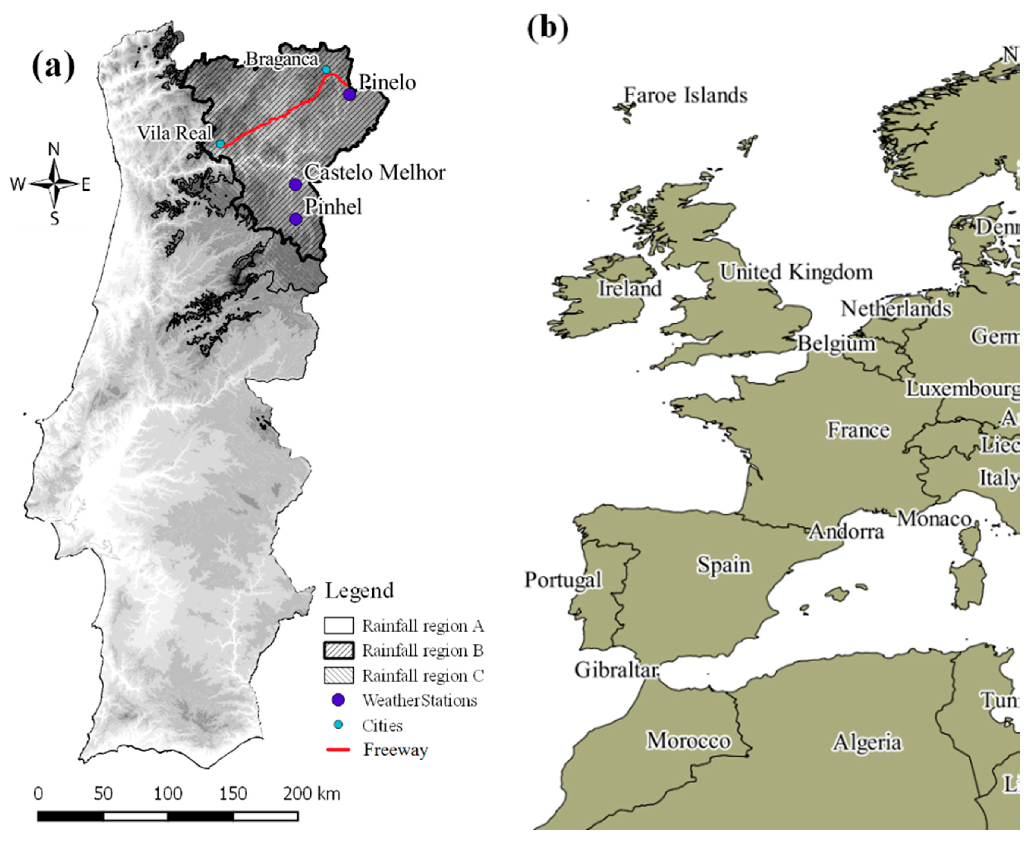
Portugal is located in the extreme southwest of Continental Europe (Figure 1a) with temperate type climate [69]. According to the Iberian Climate Atlas [70], annual average rainfall presents high spatial variability with the highest values (>2200 mm) in the mountainous areas of north-western Continental Portugal (Serra do Gerês) and the lowest values (400 mm) in the southern interior region. Monthly average rainfall presents high inter-annual variability and remarkable seasonality, more evident in the southern part of the country, characterized by: (i) Higher values (about 230 mm) in the NE corner during winter, especially in December; and (ii) the lower values (less than 5 mm) in the southern half of the country, observed during the summer months of July and August. The annual average number of days with rainfall above or equal to 10 mm also shows a strong seasonality, with the highest values of 50–75 days during winter and in a large northern area (NE and regions of central Portugal). The annual average number of days with rainfall above or equal 30 mm presents a similar spatial pattern and a strong seasonality, with the highest values (5–10 days) observed in the same season and region.

The approach adopted in this study is quite general but will be applied in the northeast region of Portugal, Figure 1a (rainfall region B) where more roads have been built recently. A section of a freeway (Auto-estrada Transmontana) which will connect two Portuguese district capitals (Vila Real and Bragança) with a total length of 186 km (130 km recently constructed) was selected as the case study (Figure 1a,b). Two distinct rainfall databases were used, namely: (i) historical observed data from the Portuguese Water Institute (SNIRH, http://snirh.pt); and (ii) RCM simulations for the recent past conditions and two future climate scenarios.

After a preliminary exploratory analysis to assess the quality of the historical time series (e.g., total number of missing values, number of months with failures), the weather stations of Castelo Melhor, Pinelo and Pinhel were selected to characterize the rainfall regime in the rainfall region B (Figure 1a). The rainfall time series contains 8 to almost 10 years of data (about 72,000 to 90,000 hourly records) and just 0% to 3.8% of missing data (

Table 1. Characteristics of the weather stations where the data used in this study were measured, including the code, name, altitude and geographical coordinates.

Name	Latitude (° N)	Longitude (° W)	Altitude (m)	Period (Year)	Missing Values (%)
Castelo Melhor	41.01	−7.06	286	2002/2008	0.0
Pinelo	41.63	−6.55	607	2003/2011	3.8
Pinhel	40.77	−7.06	606	2002/2011	1.6

). Portugal experienced significant land use/land cover changes (LULCC) in recent decades [60]. However, a recent study shows that the LULCC, especially those with higher impact on drainage coefficient (e.g., leading to the increase of the urban/artificial areas and consequently to change in soil permeability), are essentially concentrated in the central-north and south coastal areas coastal as well as in the metropolitan areas of Lisbon and Porto [71]. The LULC in study area (NE of the country) is essentially characterized by permanent crops, pastures, heterogeneous agricultural areas, scrubs and/or herbaceous vegetation associations, arable land and forests [72]. The LULCC in this region were essentially from Agricultural areas (AA) to Forest and semi natural areas (FSNA) and vice-versa [71]. This conversion between FSNA and AA appeared to be an active and dynamic process but at the country level and in relative terms, artificial surfaces registered a substantial increase of about 50%, forest and semi-natural areas remains almost constant (0.3%) and agricultural areas slightly decreased (−4.4%) [71]. The study case was developed in a rural area where substantial LULCC are not forecasted for the near future. It is, therefore, expected a conservation of runoff coefficients (C) across the study area in the short, medium and long term. The highways are characterized by C values higher than of surrounding areas but is the sole infra-structure of its kind linking the territories of Portugal and Spain in the region. For that reason, the higher C values of this road are barely capable to affect the average C within the studied region. Construction of similar infra-structures would contribute to enlarge C locally.

The rainfall projections for different future scenarios were simulated by the regional climate model Consortium for Small-Scale Modelling–Climate version of the Local Model (COSMO-CLM). This model was developed by the “COnsortium for Small-scale MOdelling” (COSMO) and the “Climate Limited-area Modelling Community” (CLM-community). COSMO-CLM has shown high ability to model weather conditions, specifically rainfall, in different regions of Europe. Consequently, this model’s simulations have been used in international projects such as PRUDENCE and ENSEMBLES [73,74] as well as in numerous climate changes’ studies [75,76,77]. The simulated rainfall was available at daily scale, on a grid of 0.2° of latitude × 0.2° of longitude for the spatial domain defined between 36.6° N–42.4° N and 6.2° W–9.8° W covering Portugal mainland. The data corresponds to three different simulations: one for the recent past conditions of the final of the 20th century (C20), for the 30-year period defined from 1971 to 2000; and two simulations corresponding to the B1 and A1B Special Report on Emissions Scenarios (SRES) [78] both covering the 21st Century. The SRES scenarios were developed to represent the driving forces and emissions described in the scenario literature, have been used to make projections of possible future climate change and were used in the IPCC Third and Fourth Assessment Report. There are four SRES storylines and scenario families [61], including: (i) The B1 which describes a more integrated and ecologically friendly convergent world with a population peak in 2050 and declining thereafter, with rapid changes in economic structures toward a service and information economy, with reductions in material intensity, the introduction of clean and resource-efficient technologies, emphasizing global solutions to economic, social, and environmental sustainability, improved equity, but without additional climate initiatives; and (ii) the A1 which describes a future world of very rapid economic growth, similar global population evolution, the rapid introduction of new and more efficient technologies, convergence among regions (in the per capita income and way of life), capacity building, extensive social and cultural interactions worldwide and (A1B) with a balance emphasis on all energy sources. Time series for the grid cells containing the locations of the weather stations previously selected (Figure 1a) were extracted.

2.2. Rainfall Disaggregation

The IDF curves need to be developed for ten different duration times, namely: 5 min, 10 min, 15 min, 30 min, 1 h, 2 h, 6 h, 12 h, 24 h and 48 h. This implies that: (i) The daily rainfall data simulated by the COSMO-CLM need to be disaggregated into sub-daily time scales; and (ii) both the simulated and observed rainfall data need to be disaggregate into sub-hourly time scales. The first disaggregation procedure was performed with the method of the fragments estimated with the observed hourly rainfall time series. A detailed description of this method may be easily found (e.g., [23,47]) but, in essence, it consists in computing and applying the various fragments defined by,

$$w_i=\frac{h_i}{d}$$

(1)

where $w_i$ represents the fragment calculated to the ith hour of the day, $h_i$ represents the value of rainfall in that hour and $d={{\displaystyle \sum }}_{i=1}^{24}{h}_i$ is the total rainfall of that day. Consequently, the sum of the fragments for each day is equal to one. Then, the disaggregation of the simulated rainfall data from daily to hourly times scales is performed by,

$$h_i^{\prime }=w_i\times d\prime$$

(2)

where $h_i^{\prime }$ is the simulated hourly rainfall for the ith hour disaggregated from the simulated daily rainfall ($d\prime$). The method of fragments has the advantage of being conservative which means that it allows performing the disaggregation preserving the total daily rainfall.

The values of the disaggregation coefficients were defined as the quotient between the values of rainfall for inferior durations in relation to the values of rainfall to higher durations. This study was not intended to cover the disaggregation of rainfall values but of maximum rainfall values. The process includes the following steps:

• Compute the maximum value of rainfall in each duration (1, 2, 6 and 12 h) on a daily basis and based on observed hourly data;
• Compute the disaggregation coefficient/fragment referring to the value of the maximum rainfall corresponding to each duration (1, 2, 6 and 12 h), for each day;
• For each duration (1, 2, 6 and 12 h) sort by descending order the disaggregation coefficient/fragments;
• Compute the mean coefficient for each duration using the first (50, 100 and 200) highest values that allows smoothing the fraction of the maximum rainfall values for the highest rainfall records for each duration.

The mean disaggregation coefficients computed for each duration reflect the relationship between the daily rainfall and the sub-daily maximum rainfall of the data observed in each season individually. The disaggregation of the rainfall for sub-hourly time scales (e.g., 5, 10, 15 and 30 min) was also performed with the methods of the fragments but, in this case, the fragments were estimated from the maps of relationships associated with the 50% percentile of maximum rainfall in 5, 10, 15, and 30 min and an hour, produced by [59]. It is important to underline that the coefficients used in this study to disaggregate the rainfall for sub-hourly scales are in line with those suggested in the Guide to Hydrological Practices of the World Meteorological Organization and studies performed by the Portuguese Institute of the Sea and the Atmosphere, which is the Portuguese Meteorological Office [56,57,58,79].

2.3. Intensity-Duration-Frequency Curves

The methodology adopted in this study for the design of IDF curves is based on [59] and described in [23]. In summary, it comprises: (i) The fitting of the extreme probability distribution function of type I (Gumbel law) to the annual time series of maximum rainfall intensity for each of the ten durations and; (ii) the linearization and subsequent regression analysis between the values of the logarithm of the intensity of the rainfall I (in mm/h) for each return period as a function of the logarithm of the rainfall duration t (in min), to estimate the values of the IDF parameters a and b, by linear regression of

$$\log \left(I\right)=\log \left(a\right)+b\times \log \left(t\right)$$

(3)

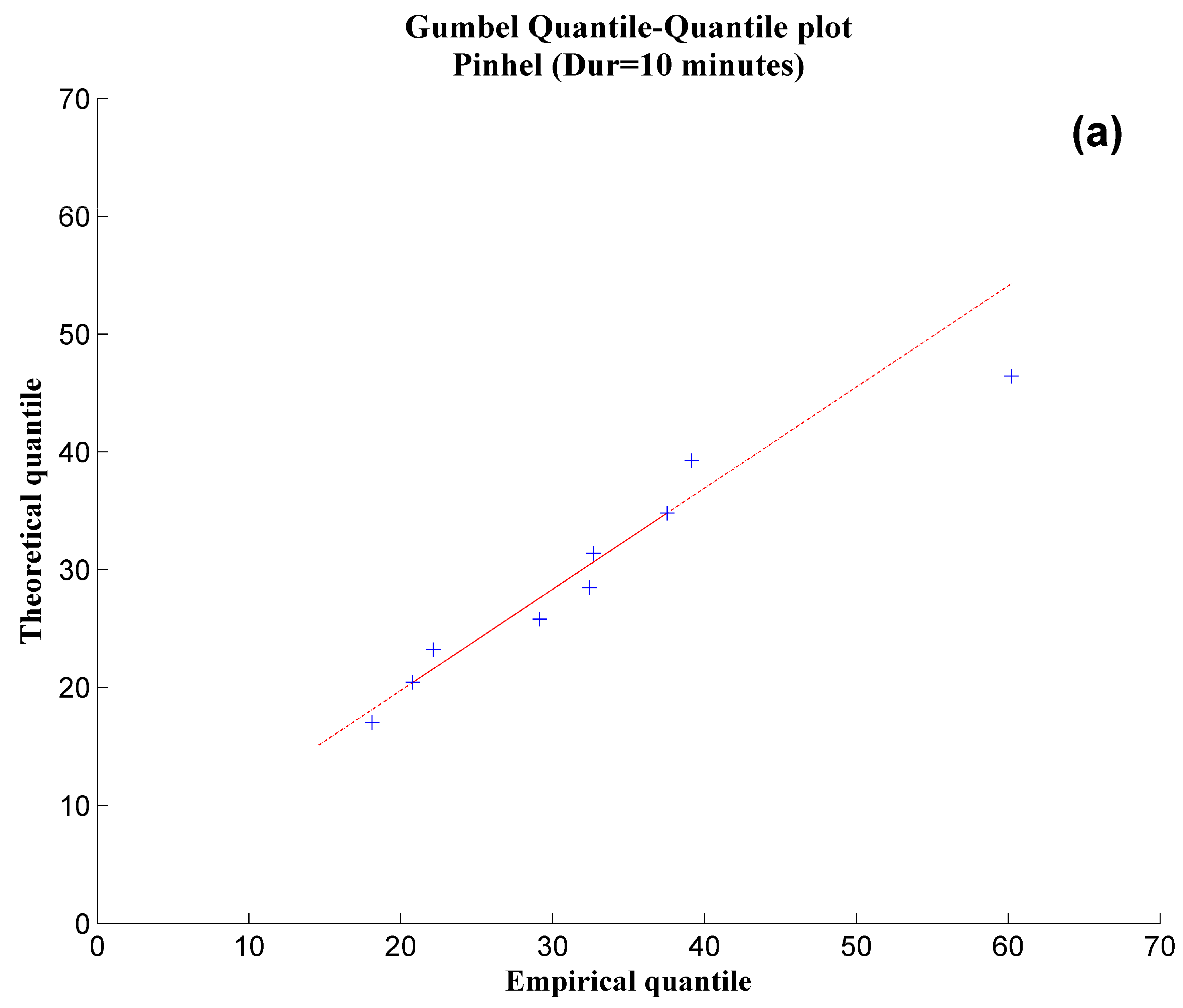
Other specificities of the methodology comprise: (i) The estimation of the Gumbel’s parameters (µ and σ) with the maximum likelihood method; (ii) the assessment of the goodness of fit of the data to the Gumbel distribution with the Kolmogorov-Smirnov test (KStest) and Quantile-Quantile (QQplot) or probability plots; and (iii) the estimation of the parameters a and b using robust regression (RR).

In general, global and regional climate models are not able to accurately reproduce the reality which results in a bias affecting the time series of the simulated meteorological variables. Consequently, the methodology includes a procedure to correct the bias in the rainfall series [80,81,82]. The bias correction is frequently performed by computing the bias between observed and simulated data for the same period (C20 scenario, in this case) and using that bias to correct the simulations for the future (B1 and A1B) scenarios [83]. Therefore, in this study the bias correction procedure consists in matching the parameters $a$ and $b$ obtained for the control scenario (C20) with those defined by law (DR) [19] and using the same factors to correct the parameters estimated for the future (FUT) scenarios as follows,

$$a_{FUTcorr}=\frac{a_{FUT}\times a_{DR}}{a_{C20}}$$

(4)

and

$$b_{FUTcorr}=\frac{b_{FUT}\times b_{DR}}{b_{C20}}$$

(5)

2.4. Design of Retention Basins

The specificities of the engineering design of retention basins (methods, procedures and data) were the following:

i.

flow rates were obtained by rational method,

$$Q_p=\frac{C\times I}{360}\times A$$

(6)

where $Q_p$ is the flood peak flow (m³/s), $C$ is the flow coefficient (dimensionless), $I$ is the rainfall intensity (mm/h) and $A$ the area of the watershed (ha). For the case study, the area of the watershed is 24.360 ha and the flow coefficient is 0.65 [84];

ii.

The rainfall intensity was calculated using the IDF curves for a duration of 15 min and a return period of 10 years, as recommended by the Drainage Manual of the contractor company of these basins;

iii.

The volume necessary to storage the effluent flow was calculated by the Dutch method, as recommended by the Portuguese legislation [19], so that the maximum flow effluent does not exceed the predetermined value obtained with Equation (6) and according to

$$V_a=10\times \left(-\frac{b\times q_s}{1+b}\right)\times {\left[\frac{60\times q_s}{a\times \left(1+b\right)}\right]}^{\frac{1}{b}}\times C\times A$$

(7)

with

$$q_s=\frac{6\times q}{C\times A}$$

(8)

where $V_a$ represents the storage volume (m³), $q_s$ is a specified effluent flow, i.e., the flow by unit of the active area of the drainage basin (mm/min), $q$ is the maximum effluent flow (m³/s), $b$ and $a$ are the parameters of the IDF curve.

3. Results and Discussion

The study was performed for periods of 30 years (1971–2000, 2011–2040, 2041–2070 and 2071–2100), which is the length of the climatological study period suggested by the World Meteorological Organization to properly characterize the climate [85]. The large number of cases studied as well as the huge amount of outputs from the curve fitting and regression analysis suggests, for sake of simplicity, to present only some of the results obtained, as illustrative examples.

The fitting of the Gumbel law to the series of maximum rainfall intensity for each of the ten durations was successfully performed with the maximum likelihood method as evidenced by the results of the KStest. Obtained results for the three weather stations (

Table 2. Results of the Gumbel distribution function fitting to time series of maximum rainfall intensity for ten different durations, using rainfall data observed in the 3 weather stations (Table 1), including: Maximum likelihood estimates of the location (μ) and scale (σ) parameters; 95% confidence interval (CI). The Kolmogorov-Smirnov statistical test was performed in all cases and the results confirm that the null hypothesis (maximum rainfall intensity is statistically distributed according to the Gumbel function) cannot be rejected at the 5% significance level (i.e., p-value < 0.05).

Weather Station	Duration	μ	CI (95%)	σ	CI (95%)
Castelo Melhor	5 min	−43.60	(−51.44; −35.76)	10.16	(5.23; 19.75)
	10 min	−31.90	(−37.64; −26.17)	7.44	(3.83; 14.45)
	15 min	−25.70	(−30.32; −21.08)	5.99	(3.08; 11.64)
	30 min	−16.73	(−19.37; −13.72)	3.90	(2.01; 7.58)
	1 h	−11.08	(−13.07; −9.09)	2.58	(1.33; 5.02)
	2 h	−7.85	(−9.12; −6.58)	1.66	(0.86; 3.21)
	6 h	−4.24	(−5.22; −3.27)	1.25	(0.70; 2.22)
	12 h	−2.66	(−3.25; −2.07)	0.74	(0.43; 1.28)
	24 h	−1.48	(−1.82; −1.14)	0.43	(0.24; 0.76)
	48 h	−0.88	(−1.02; −0.74)	0.18	(0.10; 0.32)
Pinelo	5 min	−43.66	(−50.31; −37.00)	9.72	(5.52; 17.10)
	10 min	−32.93	(−37.95; −27.91)	7.33	(4.16; 12.90)
	15 min	−25.81	(−29.75; −21.88)	5.75	(3.26; 10.11)
	30 min	−15.95	(−18.39; −13.52)	3.55	(2.02; 6.25)
	1 h	−10.16	(−11.71; −8.61)	2.26	(1.29; 3.98)
	2 h	−7.80	(−9.15; −6.44)	1.98	(1.13; 3.47)
	6 h	−4.45	(−5.12; −3.77)	0.98	(0.59; 1.63)
	12 h	−2.76	(−3.27; −2.24)	0.74	(0.44; 1.24)
	24 h	−1.69	(−1.94; −1.44)	0.36	(0.21; 0.61)
	48 h	−1.04	(−1.20; −0.89)	0.22	(0.14; 0.36)
Pinhel	5 min	−32.97	(−41.17; −24.76)	12.59	(7.64; 20.75)
	10 min	−24.98	(−31.19; −18.76)	9.54	(5.79; 15.72)
	15 min	−20.72	(−25.88; −15.56)	7.91	(4.80; 13.04)
	30 min	−13.97	(−17.44; −10.49)	5.33	(3.24; 8.79)
	1 h	−9.25	(−11.55; −6.95)	3.53	(2.14; 5.82)
	2 h	−6.70	(−8.06; −5.33)	2.10	(1.24; 3.57)
	6 h	−3.48	(−3.94; −3.02)	0.71	(0.43; 1.16)
	12 h	−2.14	(−2.51; −1.77)	0.57	(0.34; 0.94)
	24 h	−1.35	(−1.56; −1.13)	0.33	(0.19; 0.54)
	48 h	−0.82	(−0.93; −0.82)	0.17	(0.17; 0.29)

) shows KStest equal to zero for all durations, which means that the Gumbel distribution function provides a good fit to each of the series of maximum rainfall intensity. These good results are not surprising since the Gumbel distribution function have been selected to estimate IDF curves all over the world (e.g., [86,87,88,89,90]) and in the Iberian Peninsula in particular (e.g., [16,91]). Gumbel also provided the best IDF estimates for future climate conditions in Canada [92]. On the other hand, the KStest is widely used for assessing the goodness of fit in climate studies because it presents higher power than other methods for comparing robust measurement of location [93], is more efficient and less restrictive than the common chi-square test for small samples [94,95] or when the assumptions of the chi-square test are not all satisfied [96].

The quality assessment of the fit was also based on the analysis of the QQplots, which are the graphical representation of the theoretical quantiles as a function of the empirical quantiles. The closer the points are situated to the line of unit slope, the higher the quality of the fit, that is, the greater the confidence that the data fits a certain distribution [97]. As an example, the QQplots produced for the data observed in the weather station of Pinhel, for the durations of 10 min (Figure 2a) and 60 min (Figure 2b) reveals a linear and close distribution over the line $y=x$. The high quality of the fit was confirmed for all series of maximum rainfall intensity, for each of the durations, for both the observed and simulated data, and all the 30-year periods corresponding to C20, B1 and A1B scenarios.

The IDF parameters a and b are part of the linear regression results of RR and ordinary least squares (OLS). The advantage of using RR in relation to OLS method consists of reducing the effect of outliers and extremes, trying to preserve the shape, dispersion and symmetry of real data [98,99,100]. However, the analysis of the results obtained with the RR and OLS reveal residual and infrequent differences in the linear regression lines between rainfall intensity and duration. In most cases, the two regression lines appear superimposed and indistinguishable. However, a slight difference between the evolution of rainfall intensity for the durations of 30 min and 6 h was detected. In this regard, the values of the parameters a and b of the power law were estimated for all duration values simultaneously and separately for the three stretches: the first for durations of 5 to 30 min, the second between 30 min and 6 h and, the third for durations from 6 to 48 h. Also, as an example to illustrate the obtained results, values of the parameters a and b as well as of the set regression quality indicators performed with the RR for the three stations and a return period of ten years are presented in

Table 3. Values of the Intensity-Duration-Frequency (IDF) curves’ parameters a and b, estimated with robust regression and the following goodness of fit indicators: coefficient of determination (R²), F-test statistic (F-statistic) and correspondent p-value and error variance. Results for the 3 weather stations (Table 1) and return period of 10 years.

Weather Station	Duration	IDF Parameters		Quality Indicators
		a	b	R2	F-Statistic	p-Value	Error Variance
Castelo Melhor	All	186.852	−0.586	0.991	908.05219	0.00000	0.00326
	1st Excerpt	161.868	−0.535	0.993	281.45593	0.00353	0.00032
	2nd Excerpt	142.529	−0.516	0.996	442.75977	0.00225	0.00038
	3rd Excerpt	907.245	−0.818	0.996	508.68987	0.00196	0.00060
Pinelo	All	180.671	−0.581	0.995	1560.792	0.000	0.002
	1st Excerpt	171.094	−0.564	0.982	107.077	0.009	0.001
	2nd Excerpt	127.608	−0.500	0.989	180.910	0.005	0.001
	3rd Excerpt	458.768	−0.714	0.996	542.773	0.002	0.000
Pinhel	All	211.398	−0.633	0.995	1536.831	0.000	0.002
	1st Excerpt	136.223	−0.478	0.991	224.910	0.004	0.000
	2nd Excerpt	250.152	−0.656	0.996	511.454	0.002	0.001
	3rd Excerpt	314.511	−0.694	0.995	390.709	0.003	0.001

. The appropriateness of the linear behavior is substantiated by: (i) The high value of R² (greater than 99%), which measures the percentage of variance of the response variable explained by the model, for all stretches and return periods; (ii) the p-value of the F-statistic, which is the probability of rejecting the null hypothesis when it is true, is very close to zero (less than the level of 0.05) reflecting the high level of significance of the estimate [101]; and (iii) the extremely small value of the estimated error variance which confirms that the regression line is a good model for the values represented.

The volume of the retention basin was estimated by keeping unchanged all design conditions and varying only the maximum rainfall intensity (after bias correction) to ensure that differences between the volume computed for future 30-year period scenarios and C20 scenario only reflect changes in the rainfall regime. Results of the design of the retention basin for a return period of 10 years using data from the three weather stations located in the rainfall region B are shown in

Table 4. Differences in the size (relative volume change) of the retention basin for the rainfall region B, recurring to the rainfall intensity estimated with the Regulation-decree No. 23/1995 [19] (“Decreto Regulamentar No. 23/95”, DR No. 23/95 in Portuguese) and simulated data for periods of thirty years for the two future scenarios (A1B and B1).

Weather Station	Scenario	Data Period	Rainfall Intensity (mm/h)	Flow (m³/s)	Basin Volume (m3)	Volume Change (%)
Castelo Melhor	DR No. 23/95		52.50	2.31	593.20
	B1	2011–2040	64.96	2.86	733.96	24
		2041–2070	62.43	2.75	705.35	19
		2071–2100	76.61	3.37	865.53	46
	A1B	2011–2040	65.57	2.88	740.86	25
		2041–2070	61.71	2.71	697.17	18
		2071–2100	86.40	3.80	976.14	65
Pinelo	DR No. 23/95		52.50	2.31	593.20
	B1	201–2040	54.95	2.42	622.53	5
		2041–2070	60.74	2.67	620.24	5
		2071–2100	52.50	2.31	684.44	15
	A1B	2011–2040	47.27	2.08	532.69	−10
		2041–2070	52.87	2.33	597.29	1
		2071–2100	67.13	2.95	758.49	28
Pinhel	DR No. 23/95		52.50	2.31	593.20
	B1	2011–2040	61.21	2.69	691.55	17
		2041–2070	59.74	2.63	673.20	13
		2071–2100	70.26	3.09	791.75	33
	A1B	2011–2040	66.88	2.94	755.68	27
		2041–2070	52.33	2.30	589.66	−1
		2071–2100	81.85	3.60	924.80	56

. It is apparent a spatial variability between stations within the same region which could not be recognized with the design exclusively based on the Portuguese legislation which provides the same set of IDF parameter for each rainfall region.

The analysis of Table 4 reveals that, in general, the volume of the retention basin should be larger for all climate periods and scenarios. In fact, relative volume change is only negative in two cases, for the same scenario and for the first and second periods, namely: Pinelo, A1B 2011–2040; and, Pinhel, A1B 20141–2070. Coincidently, these two weather stations are located at higher and similar altitude (600 m) where the simulation of rainfall can be more affected by the model smoothed topography and spatial averaging. Nevertheless, higher relative volume changes are expected to occur in the regions of Castelo Melhor and Pinhel weather stations. This could be associated with the fact that the long-term 95th percentile of rainfall is much smaller in this region than in Pinelo while the difference between the increases is not so different [23]. Consequently, the average volume change for the three simulated periods is positive. For the B1 scenario, the average change is 30% for Castelo Melhor, 8% for Pinelo and 21% for Pinhel weather station. For the A1B scenario, the volume of the retention basin has a similar average increase of 36% for Castelo Melhor, 6% for Pinelo and 28% for Pinhel.

The increase in the volume of retention basins estimated for future climate conditions means the need to increase the capacity of existing retention basins, the construction of new larger retention basins or the construction of additional retention basins to contain and control the highest expected flood flow for the future. It is also worth noting that that the relative volume change of the retention basins is generally greater for scenario A1B than for B1 which is due to the characteristics of these climate scenarios briefly described in Section 2.1. In essence, A1B scenario (rapid convergent and economic growth and energy balanced between fossil fuels and other sources) is more severe scenario than B1 (convergence with global environmental emphasis) and, consequently, climate change impacts are usually much more significant for A1B than for B1 scenario [23].

There is also a general nonlinear increasing trend in the volume change characterized by low volume change in the interim period (2041–2070) and more significant volume increases in the late 30-year periods (2071–2100) and for the conditions of the A1B scenario. For example, in the stations of Pinelo and Pinhel the projected volume increase for the end of the XXI century is 28% and 56%, respectively, while the highest retention basin volume, corresponding to an increase of 65% (from 593.20 m³ to 976.14 m³), was obtained for Castelo Melhor. These results are also in line with the findings of previous studies [23]. In addition, our findings are in line the results of other studies with COSMO CLM model, which seems to simulate less rainfall (especially for spring months) for the same interim period in Portugal [102].

Finally, it is important to discuss some of the limitations and consequences of the data and methodology used in this study that may have some potential effect on the results and conclusions. The length of the time series of observed hourly rainfall is an important aspect of this study. Ideally, time series should be as long as possible to ensure the robustness of the results, namely estimates of specific values for return periods greater than the duration of the observed series. The quantity and quality of the data available tend to constrain the analysis and methodological procedures. This aspect is particularly important in studies evaluating the impacts of climate change, especially when the historical series are significantly shorter than the series of future projections, which could be a limiting factor of the robustness of the results and findings obtained. However, we believe that the use of official data and the methodology adopted, which includes the fit of the Gumbel distribution function to time series of rainfall intensity for different durations, and the use of the fitted distribution to generate rainfall intensity for different return periods, is able to provide robust estimate the IDF parameters, especially for the small durations and return periods required for the design of the retention basins. It is also important to underline that the spatial density of weather stations is about 3 × 10⁻⁴ stations·km⁻², of the same order of magnitude (e.g., 6.7 × 10⁻⁴ stations·km⁻² in [23]) or much higher than in other recent studies (about 9 × 10⁻⁵ stations·km⁻² in [103]; and 8.5 × 10⁻⁶ stations·km⁻² in [104]). Disaggregation of observed hourly to sub-hourly durations and simulated daily to sub-daily and sub-hourly durations using the method of the fragments implies that rainfall for shorter durations is a (fixed) fraction of rainfall for the longer durations, which has an obvious impact on the results (e.g., the similarity between some QQplots). In addition, it is assumed that rainfall patterns on sub-daily scales are predicted to be proportionally the same in future climate change scenarios, i.e., rainfall events will occur in proportion to the way they currently occur. We believe that an exhaustive assessment of how the COSMO model predicts extreme rainfall events is outside the scope and objectives of this study. Furthermore, rainfall simulations of this model have been used in different studies, namely in Portugal [23,102] including for precipitation extremes [36]. However, these aspects must be considered in the analysis and use of the results obtained.

4. Conclusions

This study focused on the validity of the design of retention basins for the control and management of storm water for different future climate change scenarios. Model’s projections for the future scenarios suggest that climate change will comprise significant modification on the distribution of extreme rainfall intensity, as suggested by several previous studies (e.g., [36,105,106]). These changes have a profound impact in the IDF curves for most periods of future scenarios and, consequently, in the design/size of retention basins. Comparing the retention basin volume computed with the IDF curves estimated for future climate scenarios and proposed by for the study region, which corresponds to rainfall region B [19], the results point to the need to increase their volume in near, mid and late future and reveal that this increase is not identical for the entire rainfall region B and more significant in the end than in the beginning of the 21st century as well as for A1B than the B1 scenario. The retention basin under study undergoes an average volume increase of around 20% during the 21st century for the conditions of B1 scenario while the correspondent average change for the A1B scenarios is even slightly higher (23%). However, maximum volume increases of the retention basin for a return period of 10 years can be of about 30% for Pinelo area and 60% for the region of Castelo Melhor and Pinhel.

In summary, the results obtained for the recent past climatic conditions and future climate scenarios suggest: (i) The existence of changes in the distribution of extreme rainfall intensity; (ii) a decrease in the return period of extreme events; (iii) high spatial variability in the rainfall within the same rainfall region; (iv) increase in the volume of the retention basins already from the near future (2011–2040); and (v) the need to discuss the eventual update of the current IDF curves in the national legislation. Despite the robustness of the methodology adopted and the quality of the database, these conclusions should be taken with caution due to some limitations imposed, such as the length of the rainfall time series observed, the minimum sampling time of one hour and the consequences of the disaggregation process.

References

- Bellu, A.; Fernandes, L.F.S.; Cortes, R.M.; Pacheco, F.A.L. A framework model for the dimensioning and allocation of a retention basin system: The case of a flood-prone mountainous watershed. J. Hydrol. 2016, 533, 567–580. [Google Scholar] [CrossRef]
- Vieira, I.; Barreto, V.; Figueira, C.; Lousada, S.; Prada, S. The use of detention basins to reduce flash flood hazard in small and steep volcanic watersheds–a simulation from Madeira Island. J. Flood Risk Manag. 2016, 11, S930–S942. [Google Scholar] [CrossRef]
- Bărăiac, O.; Arad, V. Study on sustainable landscape design and functionality of mining wastelands from jiu valley. Rev. Min./Min. Rev. 2014, 20, 21–27. [Google Scholar]
- Sébastian, C.; Barraud, S.; Gonzalez-Merchan, C.; Perrodin, Y.; Visiedo, R. Stormwater retention basin efficiency regarding micropollutant loads and ecotoxicity. Water Sci. Technol. 2014, 69, 974–981. [Google Scholar] [CrossRef] [PubMed]
- Maksimović, Č.; Kurian, M.; Ardakanian, R. Rethinking Infrastructure Design for Multi-Use Water Services; Springer International Publishing: Basel, Switzerland, 2015. [Google Scholar]
- Kim, G.; Yur, J.; Kim, J. Diffuse pollution loading from urban stormwater runoff in Daejeon city, Korea. J. Environ. Manag. 2007, 85, 9–16. [Google Scholar] [CrossRef] [PubMed]
- Muschalla, D.; Vallet, B.; Anctil, F.; Lessard, P.; Pelletier, G.; Vanrolleghem, P.A. Ecohydraulic-driven real-time control of stormwater basins. J. Hydol. 2014, 511, 82–91. [Google Scholar] [CrossRef] [Green Version]
- Yang, Q.; Shao, J.; Scholz, M.; Boehm, C.; Plant, C. Multi-label classification models for sustainable flood retention basins. Environ. Model. Softw. 2012, 32, 27–36. [Google Scholar] [CrossRef]
- Robinson, M.; Scholz, M.; Nicolas, B.; Jennifer, C. Classification of different sustainable flood retention basin types. J. Environ. Sci. 2010, 22, 898–903. [Google Scholar] [CrossRef]
- McMinn, W.R.; Yang, Q.; Scholz, M. Classification and assessment of waterbodies as adaptive structural measures for flood risk management planning. J. Environ. Manag. 2010, 91, 1855–1863. [Google Scholar] [CrossRef] [PubMed]
- Scholz, M.; Adam, J.S. Conceptual Classification Model for Sustainable Flood Retention Basins. J. Environ. Manag. 2009, 90, 624–633. [Google Scholar] [CrossRef] [PubMed]
- Liu, Y.; Bralts, V.F.; Engel, B.A. Evaluating the effectiveness of management practices on hydrology and water quality at watershed scale with a rainfall-runoff model. Sci. Total Environ. 2015, 511, 298–308. [Google Scholar] [CrossRef] [PubMed]
- Li, Y.; Zhu, G.; Ng, W.J.; Tan, S.K. A review on removing pharmaceutical contaminants from wastewater by constructed wetlands: Design, performance and mechanism. Sci. Total Environ. 2014, 468–469, 908–932. [Google Scholar] [CrossRef] [PubMed]
- Todeschini, S.; Papiri, S.; Ciaponi, C. Placement strategies and cumulative effects of wet-weather control practices for intermunicipal sewerage systems. Water Resour. Manag. 2018, 32, 2885–2900. [Google Scholar] [CrossRef]
- Todeschini, S.; Papiri, S.; Ciaponi, C. Performance of stormwater detention tanks for urban drainage systems in northern Italy. J. Environ. Manag. 2012, 101, 33–45. [Google Scholar] [CrossRef] [PubMed]
- Brandão, C. Análise de Precipitações Intensas; Dissertação para obtenção do Grau de Mestre em Engenharia Civil do Instituto Superior Técnico da Universidade Técnica de Lisboa: Lisboa, Portugal, 1995. [Google Scholar]
- Santos, G.G.; Figueiredo, C.C.; Oliveira, L.F.C.; Griebeler, N.P. Intensidade-duração-frequência de chuvas para o Estado de Mato Grosso do Sul. Rev. Bras. Eng. Agríc. Ambient. 2009, 13, 1–6. [Google Scholar] [CrossRef]
- El-Sayed, E.A.H. Generation of Precipitation Intensity Duration Frequency Curves For Ungauged Sites—Nile Basin. Water Sci. Eng. J. 2011, 4, 112–124. [Google Scholar]
- DR “Decreto Regulamentar no 23/95 (Regulation-decree no. 23/1995).” Diário da República, 194/95 (I-B).
- Moreira, M.M.; Corte-Real, J. Adaptação das Obras Hidráulicas às Alterações Climáticas; Workshop Internacional sobre Clima e Recursos Naturais nos Países de Língua Portuguesa: Ilha do Sal, Cabo Verde, 2008. [Google Scholar]
- Rosenzweig, C.; Major, D.C.; Demong, K.; Stanton, C.; Horton, R.; Stults, M. Managing climate change risks in New York City’s system: Assessment and adaptation planning. Mitig. Adapt. Strat. Glob. Chang. 2007, 12, 1391–1409. [Google Scholar] [CrossRef]
- Rosenberg, E.A.; Keys, P.W.; Booth, D.B.; Hartley, D.; Burkey, J.; Steinemann, A.C.; Lettenmaier, D.P. Precipitation extremes and the impacts of climate change on stormwater infrastructure in Washington State. Clim. Chang. 2010, 102, 319–349. [Google Scholar] [CrossRef] [Green Version]
- Pereira, M.G.; Sanches Fernandes, L.; Barros Macário, E.; Gaspar, S.; Pinto, J. Climate Change Impacts in the Design of Drainage Systems: Case Study of Portugal. J. Irrig. Drain Eng. 2014, 142, 05014009. [Google Scholar] [CrossRef]
- Todeschini, S. Trends in long daily rainfall series of Lombardia (Northern Italy) affecting urban stormwater control. Int. J. Climatol. 2012, 32, 900–919. [Google Scholar] [CrossRef]
- Christensen, J.H.; Hewitson, B.; Busuioc, A.; Chen, A.; Gao, X.; Held, I.; Jones, R.; Kolli, R.K.; Kwon, W.T.; Laprise, R.; et al. Regional Climate Projections. In Climate Change: The Physical Science Basis. Contribution of Working Group I to the 4th Assessment Report of the Intergovernamental Panel on Climate Change; Solomon, S., Qin, D., Manning, M., Chen, Z., Marquis, M., Averyt, K.B., Tignor, M., Miller, H.L., Eds.; Cambridge University Press: Cambridge, UK, 2007. [Google Scholar]
- Maraun, D.; Wetterhall, F.; Ireson, A.M.; Chandler, R.E.; Kendon, E.J.; Widmann, M.; Brienen, S.; Rust, H.W.; Sauter, T.; Themeßl, M.; et al. Precipitation downscaling under climate change: Recent developments to bridge the gap between dynamical models and the end user. Rev. Geophys. 2010, 48. [Google Scholar] [CrossRef] [Green Version]
- Cowpertwait, P.; Isham, V.; Onof, C. Point process models of rainfall: Developments for fine-scale structure. Proc. R. Soc. Lond. A 2007, 463, 2569–2587. [Google Scholar] [CrossRef]
- Jacob, D.; Bärring, L.; Christensen, O.B.; Christensen, J.H.; de Castro, M.; Deque, M.; Giorgi, F.; Hagemann, S.; Hirschi, M.; Jones, R.; et al. An inter-comparison of regional climate models for Europe: Model performance in present-day climate. Clim. Chang. 2007, 81, 31–52. [Google Scholar] [CrossRef]
- Cubasch, U.; Waszkewitz, J.; Hegerl, G.; Perlwitz, J. Regional climate changes as simulated in time-slice experiments. Clim. Chang. 1995, 31, 273–304. [Google Scholar] [CrossRef]
- Déqué, M.; Piedelievre, J.P. High resolution climate simulation over Europe. Clim. Dyn. 1995, 11, 321–339. [Google Scholar] [CrossRef]
- Wilby, R.L.; Wigley, T.M.L.; Conway, D.; Jones, P.D.; Hewitson, B.C.; Main, J.; Wilks, D.S. Statistical downscaling of general circulation model output: A comparison of methods. Water Resour. Res. 1998, 34, 2995–3008. [Google Scholar] [CrossRef] [Green Version]
- Giorgi, F.; Mearns, L.O. Introduction to special section: Regional climate modeling revisited. J. Geophys. Res. 1999, 104, 6335–6352. [Google Scholar] [CrossRef]
- Fowler, H.J.; Blenkinsop, S.; Tebaldi, C. Linking climate change modelling to impacts studies: Recent advances in downscaling techniques for hydrological modelling. Int. J. Climatol. 2007, 27, 1547–1578. [Google Scholar] [CrossRef]
- Hanssen-Bauer, I.; Achberger, C.; Benestad, R.E.; Chen, D.; Førland, E.J. Statistical downscaling of climate scenarios over Scandinavia. Clim. Res. 2005, 29, 255–268. [Google Scholar] [CrossRef] [Green Version]
- Gao, X.; Xu, Y.; Zhao, Z.; Pal, J.S.; Giorgi, F. On the role of resolution and topography in the simulation of East Asia precipitation. Theor. Appl. Climatol. 2006, 86, 173–185. [Google Scholar] [CrossRef]
- Costa, A.C.; Santos, J.A.; Pinto, J.G. Climate change scenarios for precipitation extremes in Portugal. Theor. Appl. Climatol. 2012, 108, 217–234. [Google Scholar] [CrossRef]
- Santos, F.D.; Miranda, P. Alterações Climáticas em Portugal: Cenários, Impactos e Medidas de Adaptação—Projecto SIAM II; Gradiva: Lisboa, Portugal, 2006. [Google Scholar]
- Koutsoyiannis, D.; Xanthopoulos, T. A dynamic model for short-scale precipitation disaggregation. Hydrol. Sci. J. 1990, 35, 303–322. [Google Scholar] [CrossRef]
- Rodriguez-Iturbe, I.; Cox, D.R.; Isham, V. A point process model for precipitation: Further developments. Proc. R. Soc. Lond. A 1997, 417, 283–298. [Google Scholar] [CrossRef]
- Koutsoyiannis, D.; Onof, C. A computer program for temporal rainfall disaggregation using adjusting procedures (HYETOS). In 25th General Assembly of the European Geophysical Society, Geophysical Research Abstracts; European Geophysical Society: Nice, France, 2000; Volume 2. [Google Scholar]
- Abdellatif, M.; Atherton, W.; Alkhaddar, R. Application of the stochastic model for temporal rainfall disaggregation for hydrological studies in north western England. J. Hydroinform. 2013, 15, 555–567. [Google Scholar] [CrossRef] [Green Version]
- Gaspar, S.; Macário, E.; Pereira, M.G.; Sanches Fernandes, L. Desagregação da precipitação em Portugal Continental com Hyetos. In Proceedings of the R. Física 2012, 18º Conferência Nacional de Física, 22º encontro Ibérico para o Ensino da Física, Aveiro, Portugal, 6 September 2012. [Google Scholar]
- Hanaish, I.S.; Ibrahim, K.; Jemain, A.A. Daily rainfall disaggregation using HYETOS model for Peninsular Malaysia. In Proceedings of the 5th International Conference on Applied Mathematics, Simulation, Modelling (ASM ‘11), Corfu Island, Greece, 14–16 June 2011; pp. 146–150, ISBN 978-1-61804-016-9. [Google Scholar]
- Svanidze, G.G. Principles of Estimating River Flow Regulation by the Monte Carlo Method; Metsniereba Press: Tbilisi, Georgia, 1964; p. 271. [Google Scholar]
- Svanidze, G.G. Mathematical Modeling of Hydrologic Series; for Hydroelectric and Water Resources Computations; Water Resources Publications: Fort Collins, CO, USA, 1980. [Google Scholar]
- Wey Karen, M. Temporal Disaggregation of Daily Precipitation Data in a Changing Climate; Tese apresentada à Universidade de Waterloo para obtenção do grau de mestre em Ciências Aplicadas em Engenharia Civil: Waterloo, ON, Canada, 2006. [Google Scholar]
- Gaspar, S.M. Influência das Alterações Climáticas em Bacias de Retenção; Dissertação apresentada à Universidade de Trás-os-Montes e Alto Douro para obtenção do grau de mestre em Engenharia Civil: Vila Real, Portugal, 2013. [Google Scholar]
- Wójcik, J.; Buishand, T.A. Simulation of 6-hourly rainfall and Temperature by Two Resampling Schemes. J. Hydrol. 2003, 273, 69–80. [Google Scholar] [CrossRef]
- Pui, A.; Sharma, A.; Mehrotra, R. A Comparison of Alternatives for Daily to Sub-Daily Precipitation Disaggregation. J. Hydrol. 2012, 470, 138–157. [Google Scholar] [CrossRef]
- Bernard, M.M. Formulas for precipitation intensities of long duration. Trans. ASCE 1932, 96, 592–624. [Google Scholar]
- Bell, F.C. Generalized precipitation-duration-frequency relationship. ASCE J. Hydraulic Eng. 1969, 95, 311–327. [Google Scholar]
- Chen, C.L. Precipitation intensity-duration-frequency formulas. ASCE J. Hydraulic Eng. 1983, 109, 1603–1621. [Google Scholar] [CrossRef]
- Koutsoyiannis, D.; Kozonis, D.; Manetas, A. A mathematical framework for studying precipitation intensity-duration-frequency relationships. J. Hydrol. 1998, 206, 118–135. [Google Scholar] [CrossRef]
- Okonkwo, G.I.; Mbajiorgu, C.C. Precipitation Intensity-Duration-Frequency Analyses for South Eastern Nigeria. Agric. Eng. Int. CIGR J. 2010, 12, 22–30. [Google Scholar]
- Matos, R.; Silva, M. Estudos de Precipitação com Aplicação no Projeto de Sistemas de Drenagem Pluvial. Curvas Intensidade-Duração-Frequência da Precipitação em Portugal; ITH24, LNEC: Lisboa, Portugal, 1986. [Google Scholar]
- Godinho, S. “Valores Máximos Anuais da Quantidade da Precipitação. Estimativa dos Valores Relativos a Durações Inferiores a 24 horas/Annual Maximums on the Amount of Rainfall. Estimate of Values Related to Durations less than 24 hours”; INMG: Lisbon, Portugal, 1984. [Google Scholar]
- Godinho, S. “Valores Máximos Anuais da Quantidade da Precipitação. Estimativa dos Valores Relativos a Durações Inferiores a 24 horas/Annual Maximums on the Amount of Rainfall (ii)”. Estimate of Values Related to Durations less than 24 hours”; INMG: Lisbon, Portugal, 1987. [Google Scholar]
- Godinho, S. “Valores Máximos Anuais da Quantidade da Precipitação. Estimativa dos Valores Relativos a Durações Inferiores a 24 horas/Annual Maximums on the Amount of Rainfall (ii)”. Estimate of Values Related to Durations less than 24 hours”; INMG: Lisbon, Portugal, 1989. [Google Scholar]
- Brandão, C.; Rodrigues, R.; Costa, J.P. Análise de Fenómenos Extremos, Precipitações Intensas em Portugal Continental; DSRH-INAG, Instituto da Água: Lisboa, Portugal, 2001. [Google Scholar]
- Pereira, M.G.; Aranha, J.; Amraoui, M. Land cover fire proneness in Europe. For. Syst. 2014, 23, 598–610. [Google Scholar] [CrossRef]
- Nakicenovic, N.; Alcamo, J.; Davis, G.; de Vries, B.; Fenhann, J.; Gaffin, S.; Gregory, K.; Grübler, A.; Jung, T.Y.; Kram, T.; et al. IPCC Special Report on Emissions Scenarios; Cambridge University Press: Cambridge, UK, 2000; p. 599. [Google Scholar]
- Moss, R.H.; Edmonds, J.A.; Hibbard, K.A.; Manning, M.R.; Rose, S.K.; van Vuuren, D.P.; Carter, T.R.; Emori, S.; Kainuma, M.; Kram, T.; et al. The next generation of scenarios for climate change research and assessment. Nature 2010, 463, 747–756. [Google Scholar] [CrossRef] [PubMed]
- Dufresne, J.L.; Aumont, M.-A.; Foujols, S.; Denvil, A.; Caubel, O.; Marti, O.; Balkanski, Y.; Bekki, S.; Bellenger, H.; Benshila, R.; et al. Climate change projections using the IPSL-CM5 Earth System Model: From CMIP3 to CMIP5. Clim. Dyn. 2013, 40, 2123–2165. [Google Scholar] [CrossRef] [Green Version]
- Knutti, R.; Sedláček, J. Robustness and uncertainties in the new CMIP5 climate model projections. Nat. Clim. Chang. 2013, 3, 369–373. [Google Scholar] [CrossRef]
- Stroeve, J.C.; Kattsov, V.; Barrett, A.; Serreze, M.; Pavlova, T.; Holland, M.; Meier, W.N. Trends in Arctic sea ice extent from CMIP5, CMIP3 and observations. Geophys. Res. Lett. 2012, 39, L16502. [Google Scholar] [CrossRef]
- Zhang, X.; Song, Y. Optimization of wetland restoration siting and zoning in flood retention areas of river basins in China: A case study in Mengwa, Huaihe River Basin. J. Hydrol. 2014, 519, 80–93. [Google Scholar] [CrossRef]
- Terêncio, D.P.S.; Fernandes, L.S.; Cortes, R.M.V.; Pacheco, F.A.L. Improved framework model to allocate optimal rainwater harvesting sites in small watersheds for agro-forestry uses. J. Hydrol. 2017, 550, 318–330. [Google Scholar] [CrossRef]
- Terêncio, D.P.S.; Fernandes, L.S.; Cortes, R.M.V.; Moura, J.P.; Pacheco, F.A.L. Rainwater harvesting in catchments for agro-forestry uses: A study focused on the balance between sustainability values and storage capacity. Sci. Total Environ. 2018, 613, 1079–1092. [Google Scholar] [CrossRef] [PubMed]
- Rubel, F.; Kottek, M. Observed and projected climate shifts 1901–2100 depicted by world maps of the Köppen-Geiger climate classification. Meteorol. Z. 2010, 19, 135–141. [Google Scholar] [CrossRef]
- AEMET. Iberian Climate Atlas; Agencia Estatal de Meteorología (España) and Instituto de Meteorología (Portugal): Madrid, Spain, 2011. [Google Scholar]
- Tonini, M.; Parente, J.; Pereira, M. Global assessment of land cover changes and rural-urban interface in Portugal. Nat. Hazards Earth Syst. Sci. Discuss. 2018. [Google Scholar] [CrossRef]
- Parente, J.; Pereira, M.G. Structural fire risk: The case of Portugal. Sci. Total Environ. 2016, 573, 883–893. [Google Scholar] [CrossRef] [PubMed]
- Rockel, B.; Will, A.; Hense, A. The Regional Climate Model COSMO-CLM (CCLM). Meteorol. Z. 2008, 17, 347–348. [Google Scholar] [CrossRef]
- Van der Linden, P.; Mitchell, J.F.B. ENSEMBLES: Climate Change and Its Impacts: Summary of Research and Results from the ENSEMBLES Project; Met Office Hadley Centre: Exeter, UK, 2009; p. 160. [Google Scholar]
- Dobler, A.; Ahrens, B. Four climate change scenarios for the Indian summer monsoon by the regional climate model COSMO-CLM. J. Geophys. Res. 2011, 116, D24104. [Google Scholar] [CrossRef]
- Haslinger, K.; Anders, I.; Hofstätter, M. Regional Climate Modelling over complex terrain: An evaluation study of COSMO-CLM hindcast model runs for the Greater Alpine Region. Clim. Dyn. 2013, 40, 511–529. [Google Scholar] [CrossRef]
- Kotlarski, S.; Bosshard, T.; Lüthi, D.; Pall, P.; Schär, C. Elevation gradients of European climate change in the regional climate model COSMO-CLM. Clim. Chang. 2012, 112, 189–215. [Google Scholar] [CrossRef]
- Nakicenovic, N.; Swart, R. Special Report on Emissions Scenarios; Nakicenovic, N., Robert Swart, R., Eds.; Cambridge University Press: Cambridge, UK, 2000; p. 612. ISBN 0521804930. [Google Scholar]
- World Meteorological Organization (WMO). Guide to Hydrological Practice: Data Acquisition and Processing, Analysis, Forecasting and Other Applications; WMO: Geneva, Switzerland, 1994. [Google Scholar]
- Kilsby, C.G.; Jones, P.D.; Burton, A.; Ford, A.C.; Fowler, H.J.; Harpham, C.; James, P.; Smith, A.; Wilby, R.L. A daily weather generator for use in climate change studies. Environ. Model. Softw. 2012, 22, 1705–1719. [Google Scholar] [CrossRef]
- Davin, E.L.; Stockli, R.; Jaeger, E.B.; Levis, S.; Seneviratne, S.I. COSMO-CLM2: A new version of the COSMO-CLM model coupled to the Community Land Model. Clim. Dyn. 2011, 37, 1889–1907. [Google Scholar] [CrossRef]
- Pereira, M.G.; Calado, T.J.; Da Camara, C.C.; Calheiros, T. Effects of regional climate change on rural fires in Portugal. Clim. Res. 2013, 57, 187–200. [Google Scholar] [CrossRef] [Green Version]
- Fowler, H.J.; Kilsby, C.G. Using regional climate model data to simulate historical and future river flows in northwest England. Clim. Chang. 2007, 80, 337–367. [Google Scholar] [CrossRef]
- Chow, V.T. Handbook of Applied Hydrology; McGraw-Hill: New York, NY, USA, 1964. [Google Scholar]
- Intergovernmental Panel on Climate Change (IPCC). Managing the Risks of Extreme Events and Disasters to Advance Climate Change Adaptation. A Special Report of Working Groups I and II of the Intergovernmental Panel on Climate Change; Field, C.B., Barros, V., Stocker, T.F., Qin, D., Dokken, D.J., Ebi, K.L., Mastrandrea, M.D., Mach, K.J., Plattner, G.-K., Allen, S.K., et al., Eds.; Cambridge University Press: Cambridge, UK; New York, NY, USA, 2012. [Google Scholar]
- Dame, R.d.C.F.; Teixeira, C.F.A.; Terra, V.S.S. Comparison of different methodologies to estimate intensity-duration-frequency curves for pelotas—RS, Brazil. Eng. Agric.-Jaboticabal. 2008, 28, 245–255. [Google Scholar] [CrossRef]
- Ariff, N.M.; Jemain, A.A.; Ibrahim, K.; Zin, W.Z.W. IDF relationships using bivariate copula for storm events in Peninsular Malaysia. J. Hydrol. 2012, 470, 158–171. [Google Scholar] [CrossRef]
- Ben-Zvi, A. Rainfall intensity-duration-frequency relationships derived from large partial duration series. J. Hydrol. 2009, 367, 104–114. [Google Scholar] [CrossRef]
- Kuo, C.-C.; Gan, T.Y.; Chan, S. Regional Intensity-Duration-Frequency Curves Derived from Ensemble Empirical Mode Decomposition and Scaling Property. J. Hydrol. Eng. 2013, 18, 66–74. [Google Scholar] [CrossRef]
- Lumbroso, D.M.; Boyce, S.; Bast, H.; Walmsley, N. The challenges of developing rainfall intensity-duration-frequency curves and national flood hazard maps for the Caribbean. J. Flood Risk Manag. 2011, 4, 42–52. [Google Scholar] [CrossRef]
- Llasat, M.C. An objective classification of rainfall events on the basis of their convective features: Application to rainfall intensity in the northeast of Spain. Int. J. Climatol. 2001, 21, 1385–1400. [Google Scholar] [CrossRef]
- Das, S.; Millington, N.; Simonovic, S.P. Distribution choice for the assessment of design rainfall for the city of London (Ontario, Canada) under climate change. Can. J. Civ. Eng. 2013, 40, 121–129. [Google Scholar] [CrossRef]
- Wilcox, R.R. Some practical reasons for reconsidering the Kolmogorov-Smirnov test. Br. J. Math. Stat. Psychol. 1997, 50, 9–20. [Google Scholar] [CrossRef]
- Campos, H. Estatística Não Paramétrica, 4th ed.; ESALQ/USP: Piracicaba, Brazil, 1983; p. 349. [Google Scholar]
- Horn, S.D. Goodness-of-fit tests for discrete data: A review and an application to a health impairment scale. Biometrics 1977, 33, 237–247. [Google Scholar] [CrossRef] [PubMed]
- Mitchell, B. A comparison of chi-square and Kolmogorov-Smirnov tests. Area 1971, 3, 237–241. [Google Scholar]
- Hartmann, M.; Moala, F.A.; Mendonça, M.A. Estudo das precipitações máximas anuais em Presidente Prudente. Rev. Bras. Meteorol. 2011, 26, 561–568. [Google Scholar] [CrossRef]
- Li, G. Robust regression. In Exploring Data Tables, Trends, and Shapes; Hoaglin, D.C., Mosteller, C.F., Tukey, J.W., Eds.; Wiley: New York, NY, USA, 1985; pp. 281–340. [Google Scholar]
- Montgomery, D.C.; Peck, E.A.; Vining, G.G. Introduction to Linear Regression Analysis; John Wiley & Sons: Hoboken, NJ, USA, 2012; Volume 821. [Google Scholar]
- Phillips, G.R.; Eyring, E.M. Comparison of conventional and robust regression in analysis of chemical data. Anal. Chem. 1983, 55, 1134–1138. [Google Scholar] [CrossRef]
- Matos, M.A. Manual Operacional para a Regressão Linear; FEUP: Porto, Portugal, 1995. [Google Scholar]
- Santos, J.A.; Malheiro, A.C.; Karremann, M.K.; Pinto, J.G. Statistical modelling of grapevine yield in the Port Wine region under present and future climate conditions. Int. J. Biometeorol. 2011, 55, 119–131. [Google Scholar] [CrossRef] [PubMed]
- Mirhosseini, G.; Srivastava, P.; Stefanova, L. The impact of climate change on rainfall Intensity–Duration–Frequency (IDF) curves in Alabama. Reg. Environ. Chang. 2013, 13, 25–33. [Google Scholar] [CrossRef]
- Mohymont, B.; Demarée, G.R.; Faka, D.N. Establishment of IDF-curves for precipitation in the tropical area of Central Africa-comparison of techniques and results. Nat. Hazards Earth Syst. Sci. 2004, 4, 375–387. [Google Scholar] [CrossRef]
- Panferov, O.; Sogachev, A.; Ahrends, B. Changes of Forest Stands Vulnerability to Future Wind Damage Resulting from Different Management Methods. Open Geogr. J. 2010, 3, 80–90. [Google Scholar] [CrossRef]
- Ahrends, B.; Penne, C.; Panferov, O. Impact of Target Diameter Harvesting on Spatial and Temporal Pattern of Drought Risk in Forest Ecosystems Under Climate Change Conditions. Open Geogr. J. 2010, 3, 91–102. [Google Scholar] [CrossRef]
Figure 1.
Location of (a) the highway “Auto-Estrada Transmontana” linking two Portuguese districts’ capitals (Vila Real and Bragança), three rainfall regions legally defined for Portugal by [55], three weather stations within rainfall region B and (b) of Portugal in western Europe.
Figure 2.
QQplots produced for the data observed in the weather station of Pinhel, for the durations of 10 min (a) and 60 min (b).