An Integration Approach for Mapping Field Capacity of China Based on Multi-Source Soil Datasets

Abstract

Field capacity is one of the most important soil hydraulic properties in water cycle, agricultural irrigation, and drought monitoring. It is difficult to obtain the distribution of field capacity on a large scale using manual measurements that are both time-consuming and labor-intensive. In this study, the field capacity ensemble members were established using existing pedotransfer functions (PTFs) and multiple linear regression (MLR) based on three soil datasets and 2388 in situ field capacity measurements in China. After evaluating the accuracy of each ensemble member, an integration approach was proposed for estimating the field capacity distribution and development of a 250 m gridded field capacity dataset in China. The spatial correlation coefficient (R) and root mean square error (RMSE) between the in situ field capacity and ensemble field capacity were 0.73 and 0.048 m³·m⁻³ in region scale, respectively. The ensemble field capacity shows great consistency with practical distribution of field capacity, and the deviation is revised when compared with field capacity datasets provided by previous researchers. It is a potential product for estimating field capacity in hydrological and agricultural practices on both large and fine scales, especially in ungauged regions.

1. Introduction

There is an urgent demand for high-precision soil information data due to the increase of environmental, ecological, and food problems [1,2]. As a critical soil property, field capacity is defined as the volumetric water content retained in a uniform soil profile, two or three days after having been completely wetted with water and after free drainage beyond the root zone has become negligible [3,4]. It is a critical parameter of soil hydraulic properties for runoff, evaporation, and infiltration calculations in a land surface model and is applied in the determination of agricultural irrigation and drought monitoring indicators [5,6,7,8]. In large scale hydrology, drought, and agriculture studies, accurate field capacity data is essential [9].

Various approaches have been used to obtain the field capacity and its distribution, among which the pedotransfer functions (PTFs) are the most widely used and effective [10,11]. For field measurements, PTFs are used to transfer most basic soil information, such as soil texture, structure, and pH into other more laborious and expensively determined soil properties, such as hydraulic conductivity and field capacity [12]. Multiple linear regression (MLR) and artificial neural networks (ANNs) are usually used as techniques to build up PTFs [13,14,15,16]. For large scale research, PTFs are also used to map the distribution of laboriously measured soil properties based on basic soil information maps. Reynolds et al. [17] developed a worldwide field capacity distribution for 10 km grids using the PTFs based on the digital soil map of the world from the Food and Agriculture Organization of the United Nations (FAO). Dai et al. [18] calculated the field capacity for 1 km grids in China using a median of ten established PTFs based on the soil dataset released by Beijing Normal University (BNU). Sun and Yang [19] used the numerical approach along with PTFs to map the distribution of field capacity in China using contour diagrams.

The above-mentioned researches have improved our understanding of the spatial distribution of field capacity in China. However, there are still some problems to be solved. First, the PTFs adopted in the researches were developed using soil profiles sampled outside of China [20,21], and therefore, the variation in the climate and soil type would certainly cause uncertainty in the application of these PTFs in China [22]. Second, most of previous studies used soil properties from a single soil dataset, either FAO or BNU, to calculate the field capacity [17,23,24], and the accuracy of the results was influenced by the accuracy of the soil dataset itself. Third, most previous studies lacked the validation work using the in situ field capacity, which may increase the uncertainty in the application of the field capacity dataset [17,18]. Thus, the method for how to build a reliable field capacity dataset on a large scale in China is still to be investigated.

The aim of this study is to solve the aforementioned problems and investigate how to develop a reliable field capacity product in China. In this study, the in situ field capacity of 2388 stations were measured as the reference data. The in situ field capacity is first used to evaluate the suitability of the existing PTFs for calculating field capacity. The ensemble members [25,26] of field capacity is then built using existing PTFs and new PTFs developed by MLR method. On this basis, an integration approach was proposed to simulate the field capacity distribution for 250 m grids based on multi-source soil datasets. Lastly, we analyze the spatial characteristics of the field capacity distribution in China and validate the ensemble field capacity.

2. Materials and Methods

2.1. Study Area and Data

2.1.1. Study Area

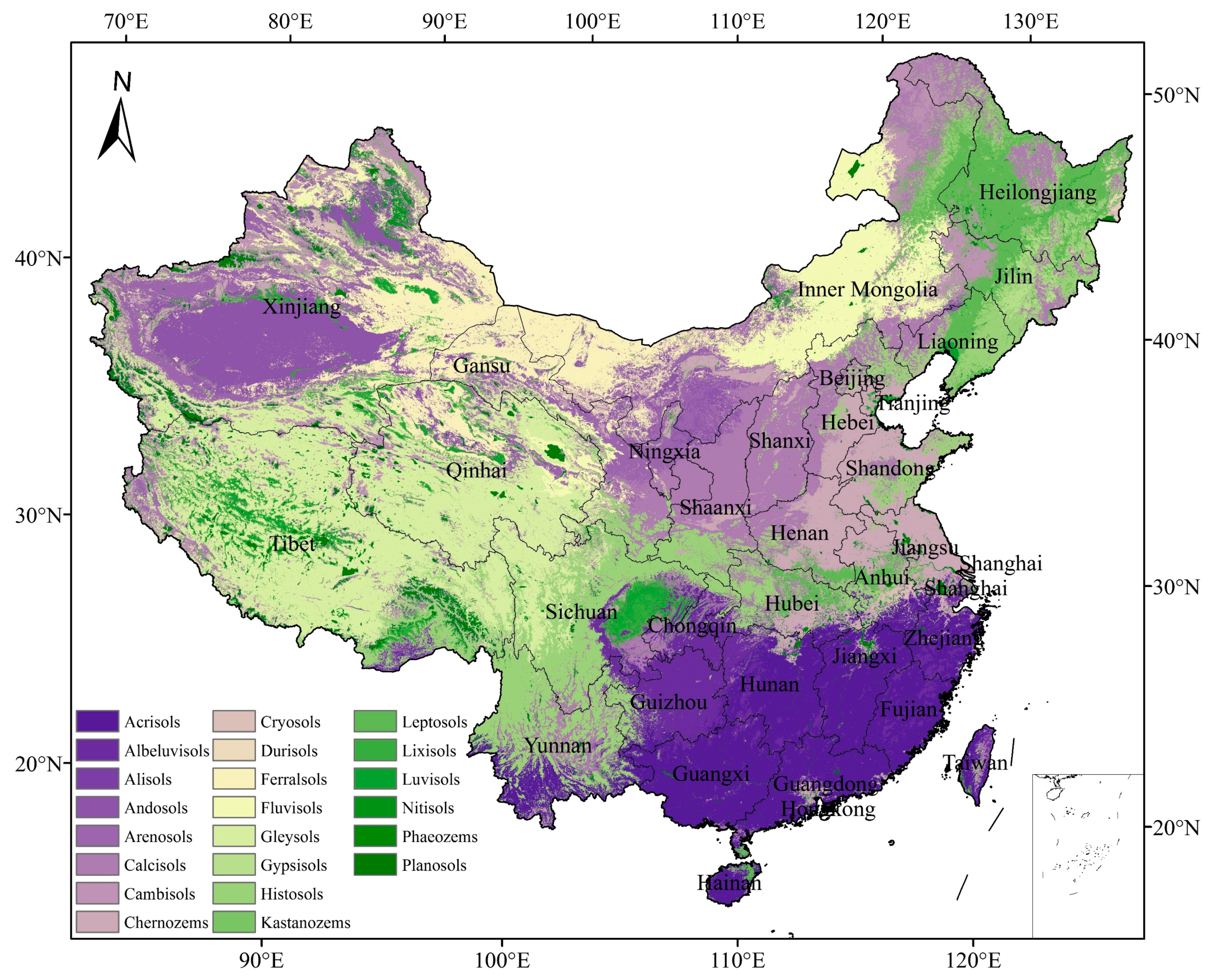
China is located in the eastern part of the Eurasian continent with a land area greater than 9.6 million km². In general, it is composed of three ladders with increasing altitude from eastern plains to western Tibetan Plateau [27] and has complex climates (e.g., monsoon climate, temperate continental climate, and alpine climate) [28]. The annual average temperature is 9.6 °C, and the annual precipitation ranges from 2000 mm in the southeast to 50 mm in the northwest [29]. Figure 1 shows a map of soil types from SoilGrids [30] (https://soilgrids.org/) classified according to the World Reference Base [31].

2.1.2. In Situ Field Capacity

The in situ field capacity data was obtained from the Ministry of Water Resources of China. The in situ field capacity values were measured using a time-based method [19] at 2388 stations, i.e., soil samples were artificially wetted to saturation and the mass of soil samples was measured every hour. When the mass difference between the two measurements was less than 0.5 g, then the soil moisture of the sample is measured and considered as the field capacity. At each station, soil samples were collected from depths of 0–10 cm, 10–20 cm, and 20–40 cm, respectively, and the in situ field capacity was calculated as a weighted average using Equation (1):

$$\overline{FC}=\frac{{{\displaystyle \sum }}_{i=1}^3\left(F{C}_i\times h_i\right)}{H}$$

(1)

where FC_i is the field capacity measured at the i depth, h_i is the representative thickness of the i depth, and H is the thickness of the entire soil sample.

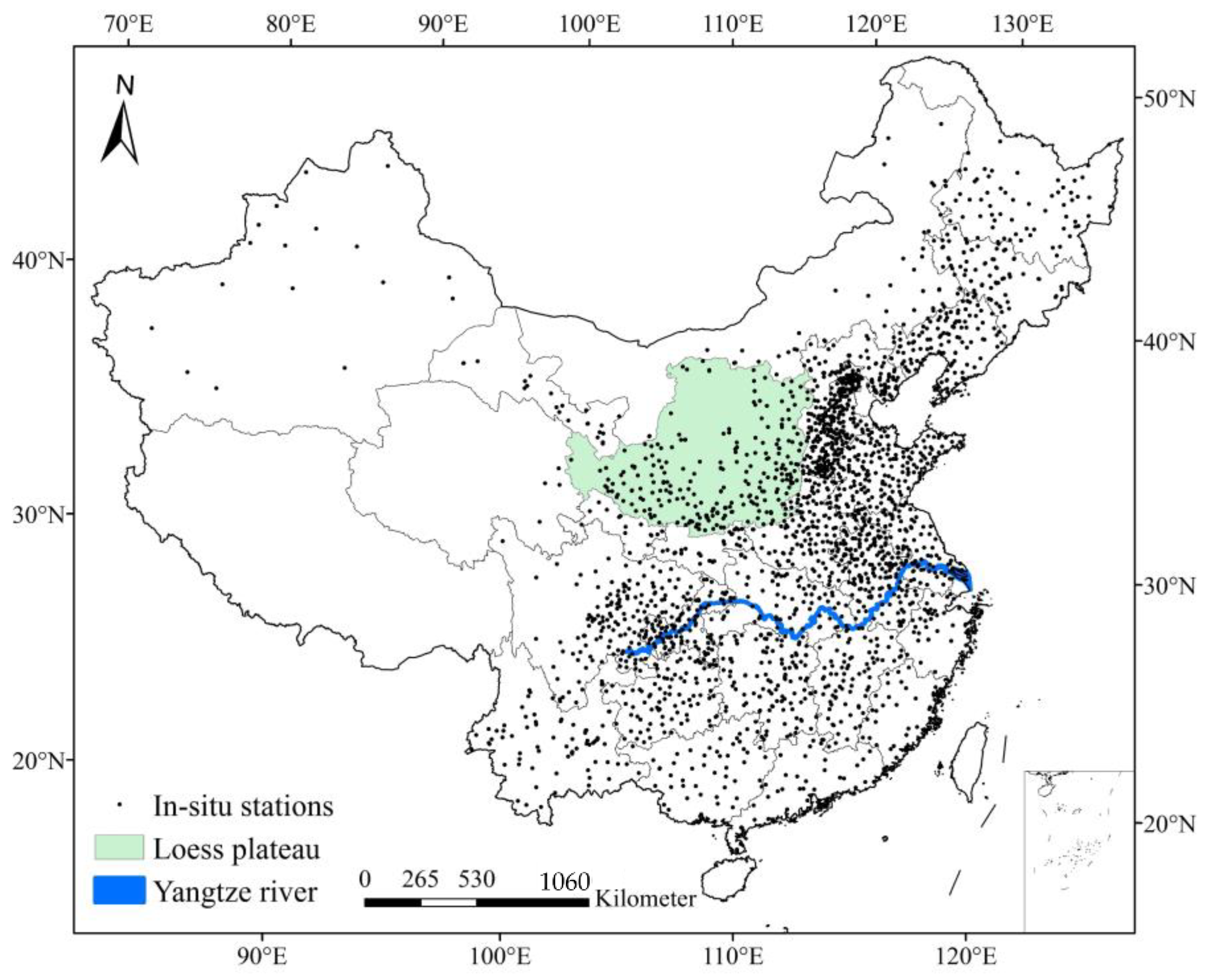
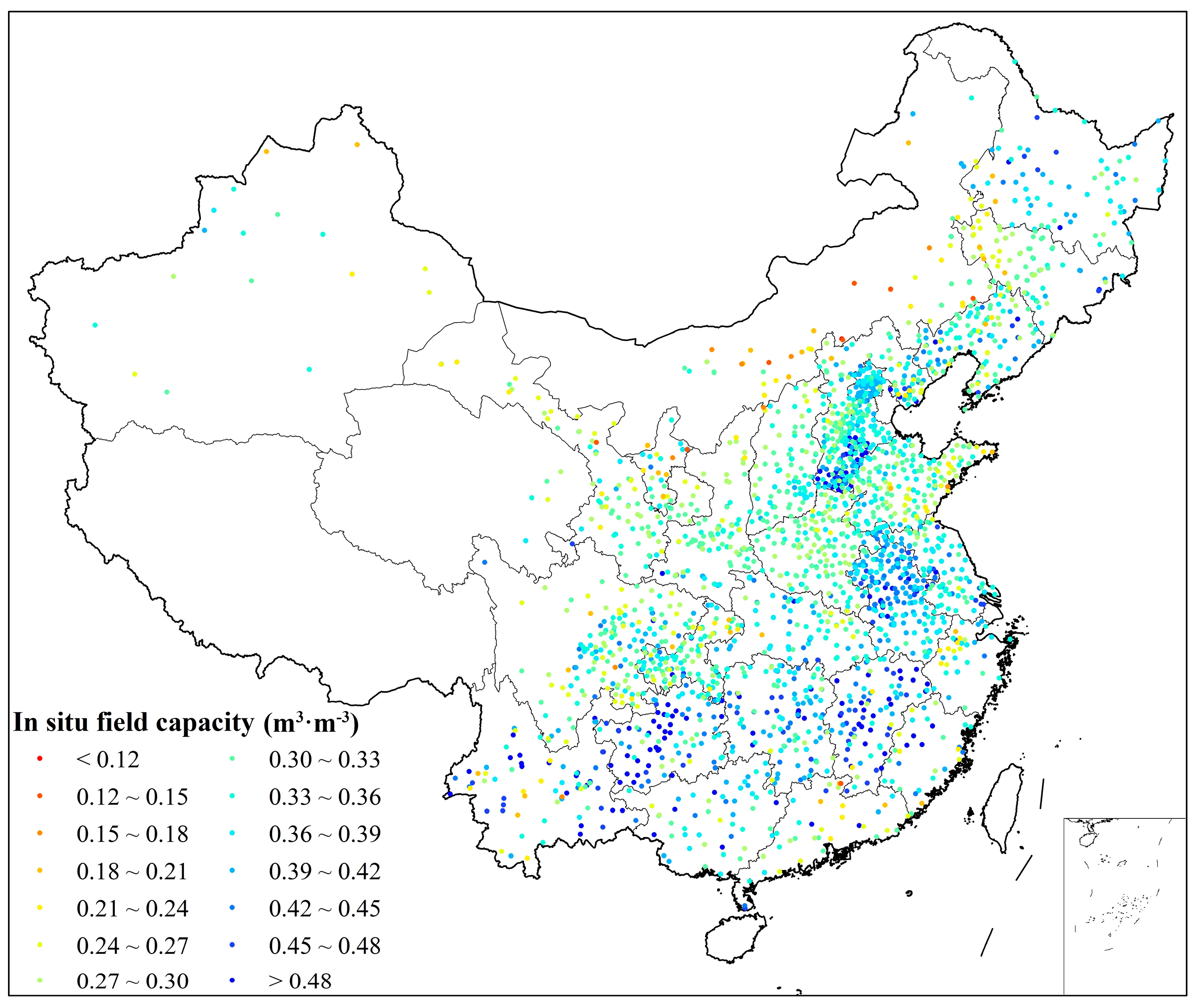
In total, 2388 in situ station-based measurements of the field capacity were adopted in this paper. Figure 2 shows the distribution of the 2388 stations in China. The stations covered the entire study area comprehensively with the exclusion of the Qinghai–Tibet Plateau, northern Inner Mongolia province, and southern Xinjiang province.

2.1.3. FAO Dataset

Reynolds et al. [17] developed a 10 km gridded soil dataset (hereafter FAO dataset) (http:// fao.org/soils-portal/) based on the FAO soil database and World Inventory of Soil Emission potentials (WISE). The dataset included soil texture (e.g., sand content, clay content, silt content), soil organic matter (SOM), and soil bulk density (BD). The soil in the dataset was divided into two layers, 0–30 cm for the upper layer and 30–100 cm for the lower layer. A variety of soil datasets were developed based on the FAO dataset, e.g., the harmonized world soil database (HWSD) in 2009 and more recently the WISE30sec [32], which demonstrated its robustness and reliability in obtaining the large-scale distribution of soil properties [33].

2.1.4. BNU Dataset

Dai et al. [18] collected 8595 soil profiles from the second national soil survey and reclassified the soil profiles into consistent soil types [34]. Based on these representative soil profiles and a 1:1,000,000 soil map of China, Dai et al. [18] calculated 1 km gridded soil characteristics datasets using the polygon link method (http://westdc.westgis.ac.cn/). The soil dataset (hereafter BNU dataset) included several soil properties (e.g., sand, clay, silt, SOM, BD, and pH). The vertical variation of the dataset was captured by using seven-layer depths, i.e., 0–4.5 cm, 4.5–9.1 cm, 9.1–16.6 cm, 16.6–28.9 cm, 28.9–49.3 cm, 49.3–82.9 cm, and 82.9–138.3 cm [35]. Hu et al. [36] used the BNU dataset to calculate the 1 km spatiotemporal distribution of evapotranspiration in the Heihe River basin in northwest China and proved its robustness in China.

2.1.5. SoilGrids Dataset

SoilGrids (http://soilgrids.org) is the most recent globally complete soil information dataset currently available, released by the International Soil Reference and Information Center (ISRIC). This dataset was driven by globally distributed soil profiles data modeled relative to environmental co-variables. In 2015, the 1.0 version of SoilGrids dataset, produced based on geostattistics, provided the 1 km gridded maps of physical soil properties (e.g., sand, clay, silt, BD, coarse fragments), bio-chemical soil properties (i.e., SOM, soil pH and cation exchange capacity), and soil classification map [37]. In version 2.0, which was produced based on machine learning and released in 2016, the resolution was further improved from 1 km to 250 m as well as the accuracy [30]. The soil in the SoilGrids dataset (hereafter SG dataset) was divided into six layers from top to bottom at depths of 0–5 cm, 5–15 cm, 15–30 cm, 30–60 cm, 60–100 cm, and 100–200 cm. As a global statistical model, the SG dataset provided an estimate of the soil properties, biased solely by the bias in the soil profiles data available and used on a global scale. At the regional scale, the SG dataset can be used as auxiliary variables to improve the estimation of the soil hydraulic parameters [37], as shown for sub-Saharan Africa by Leenarars et al. [38], which is the theoretical foundation of the following downscale algorithm in this paper. Mantel et al. [39] validated the dataset to ensure the robustness in its application.

Table 1. Summary of soil datasets in China, the number in parentheses represents the publication year of the dataset: global soil data task (GSDT); coarse fragments (CF); cation exchange capacity (CEC); total nitrogen (TN); total phosphorus (TP); basic saturation (BS); saturated volumetric water content (SWC); field capacity (FC).

Soil Dataset	Resolution	Depths (cm)	Soil Properties
FAO (2000)	10 km × 10 km	0–30, 30–100	Sand, clay, silt, SOM, BD, pH, FC
SG (2017)	250 m × 250 m	0–5, 5–15, 15–30, 30–60, 60–100, 100–200	Sand, clay, silt, SOM, BD, CF, pH, CEC
BNU (2013)	1 km × 1 km	0–4.5, 4.5–9.1, 9.1–16.6, 16.6–28.9, 28.9–49.3, 49.3–82.9, 82.9–138.3	Sand, clay, silt, SOM, BD, FC, TN, TP, etc.
HWSD (2014)	1 km × 1 km	0–30, 30–100	Sand, clay, silt, SOM, BD, BS, etc.
GSDT [40] (2000)	10 km × 10 km	0–30, 30–100	Sand, clay, silt, SWC, etc.

summarizes the recent soil datasets in China and the information corresponding to resolution, depths and soil properties.

2.2. Methods

In this paper, an integration approach was proposed to estimate the 250 m gridded field capacity in China. The approach mainly involved two steps: Establishing the field capacity ensemble members and estimating the field capacity based on those ensemble members.

2.2.1. Establishment of Field Capacity Ensemble Members

As the three datasets have different grid resolutions and grid positions, the SG 250 m grid was first defined as the benchmark grid and the FAO and BNU datasets were then resampled to the benchmark grid using nearest neighbor interpolation. In addition, owing to the inconsistent layers of soil in the three datasets, the layer closest to the soil depth of the in situ field capacity (0–40 cm) was selected, i.e., 0–30 cm for the FAO, 0–28.9 cm for the BNU, and 0–30 cm for the SG datasets. Data were calculated by weighted average method (Equation (1)).

Each station was matched up with the benchmark grid using the nearest neighbor method and obtained station-based soil properties from three datasets, respectively. For each station, we calculated the field capacity using seven existing PTFs based on the three datasets, and 21 groups of field capacity ensemble members were then obtained. The details of the seven PTFs are shown as follows. The sand, silt, and clay denote percentages (%) of textural fractions according to the USDA textural classification. SOM is the soil organic matter content (g/1000 g), and BD is the bulk density (g·m⁻³).

PTF1 [41]:	$fc=\left(0.043+0.004\times clay\right)/\left(0.471+0.00411\times clay\right)$
PTF2 [42]:	$\begin{array}{ll}fc=& 0.01\times BD\times [2.65+1.105\times clay-0.018968\times cla{y}^2+0.0001678\times cla{y}^3+\\ & 15.12\times BD-6.745\times B{D}^2-0.1975\times \left(clay\right)\times \left(BD\right)]\end{array}$
PTF3 [43]:	$\begin{array}{ll}fc=& 0.003075\times sand+0.005886\times silt+0.008039\times clay+0.002208\times SOM-\\ & 0.1434\times BD\end{array}$
PTF4 [44]:	$fc=0.2081+0.0045\times clay+0.0013\times silt-0.0595\times BD$
PTF5 [45]:	$fc=0.1183+0.0096\times clay-0.00008\times cla{y}^2$
PTF6 [46]:	$fc=0.04046+0.00426\times silt+0.00404\times clay$
PTF7 [21]:	$\begin{array}{ll}a=& \exp [-4.396-0.0715\times clay-4.88\times {10}^{-4}\times san{d}^2-4.285\times {10}^{-5}\times \left(san{d}^2\right)\times \\ & \left(clay\right)]\\ b=\hfill & -3.14-0.00222\times clay-3.484\times {10}^{-5}\times \left(san{d}^2\right)\times \left(clay\right)\\ fc=\hfill & {\left(0.33/a\right)}^{\left(1/b\right)}\end{array}$

Moreover, considering the suitability of these PTFs in China, we also developed new PTFs using MLR between the in situ field capacity and soil properties (i.e., sand content, clay content, silt content, bulk density, and soil organic matter) based on the three datasets. Different ratios of training and testing data (90%/10%, 80%/20%, 70%/30%, 60%/40%) were attempted. It was found that the regression model was quite stable and reliable (with the increase of training data, the training R decreased slightly while the test R increased largely). Thus, it is suitable to use all the in situ field capacity values for training the regression model in order to realize an optimal prediction ability. ANNs were also used to train PTFs, however, the performance showed a slight difference considering R (approximately 5%) from that obtained with MLR. To simplify the calculation and reduce the calculation time, only MLR was used as a training model. Together with the three groups of MLR results (i.e., FAO, BNU, and SG) to the former 21 ensemble members, a total of 24 groups of field capacity ensemble members were finally obtained. For each ensemble member, the standard deviation (σ), mean values (mean), coefficient of variance (CV), R, and RMSE between the ensemble members and in situ field capacity were calculated.

In practice, different multiple regression equations can be determined for different regions. It is also feasible to establish a regression field capacity group using several multiple regressions corresponding to the various regions of China. It has been demonstrated that the precision of this method is superior to that obtained when using only one multiple regression equation. However, as we are focused more on the larger scale study, in this study, we decided to use only one multiple regression equation for each dataset for the whole of China to make the integration approach simple and robust. Theoretically, region-specific regression would increase the field capacity estimation accuracies and the related researches can be carried out in the future.

2.2.2. Integration of Ensemble Members

The commonly used integration approaches are the average method, weighted averaged method, and machine learning method [21]. In this paper, we proposed an integration approach based on statistical indicators. The deterministic coefficients (R²) were used as the weight factors, and the R and RMSE were used as evaluation metrics. The calculation formulas are as follows, i represents each station, n represents total number of stations, x represents in situ field capacity, and y represents estimated field capacity:

$$\mathrm{R}=\frac{{{\displaystyle \sum }}_{i=1}^n\left(x_i-\overline{x}\right)\left(y_i-\overline{y}\right)}{\sqrt{{{\displaystyle \sum }}_{i=1}^n{\left(x_i-\overline{x}\right)}^2}\sqrt{{{\displaystyle \sum }}_{i=1}^n{\left(y_i-\overline{y}\right)}^2}}$$

(2)

$$\mathrm{RMSE}=\sqrt{\frac{{{\displaystyle \sum }}_{i=1}^n{\left(x_i-y_i\right)}^2}{n}}$$

(3)

First, the R² of the ensemble members were used as the weight factors, and the results were then revised according to the ratio of standard deviation. Finally, each ensemble member was added and the bias between the average field capacity of the weighted ensemble members and the in situ field capacity was subtracted. After the integration process, the unbiased field capacity estimation for the whole of China was obtained. In the following formulas, i represents the ensemble member, n represents the number of ensemble members, σ represents the standard deviation, R² represents the deterministic coefficient, $\overline{f{c}_i}$ represents the average values of the corresponding field capacity groups, obs represents the observed field capacity, and fc_ensemble represents ensemble field capacity:

$$f{c}_{ensemble}={\displaystyle \sum }_{i=0}^n\frac{{\sigma }_{obs}}{{\sigma }_i}\times \frac{R_i^2}{{{\displaystyle \sum }}_{i=0}^n{R}_i^2}\times f{c}_i-\Delta fc$$

(4)

$$\Delta fc={\displaystyle \sum }_{i=0}^n\frac{{\sigma }_{obs}}{{\sigma }_i}\times \frac{R_i^2}{{{\displaystyle \sum }}_{i=0}^n{R}_i^2}\times \overline{f{c}_i}-\overline{f{c}_{obs}}$$

(5)

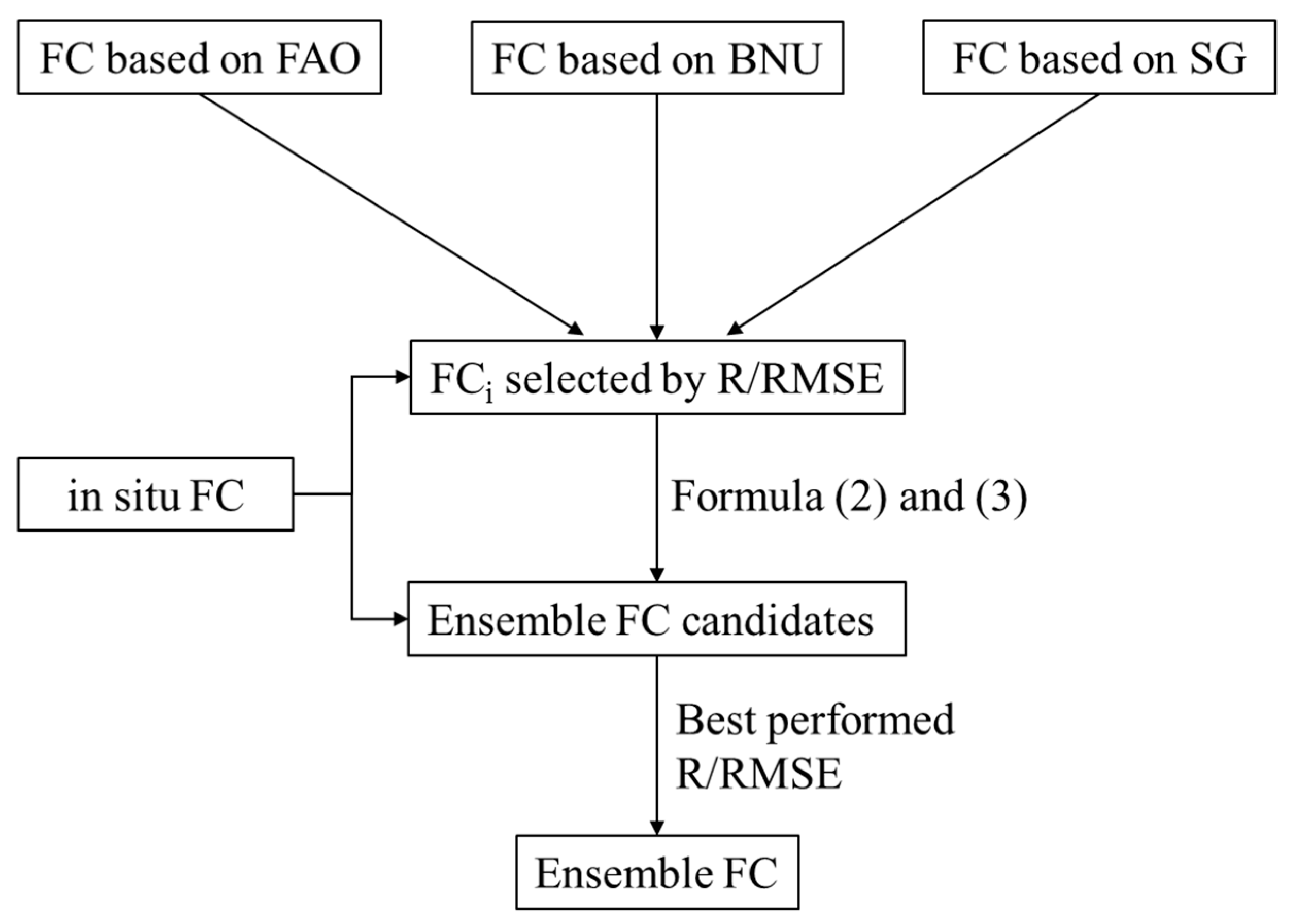
In order to determine the best combination to establish ensemble field capacity, an algorithm (Figure 3) was designed. First, three ensemble members (one for each soil dataset) were selected considering the R and RMSE values. Then the ensemble field capacity candidates were calculated using Equations (4) and (5), and they are validated with the in situ field capacity. R and RMSE were considered as two evaluation indicators for each combination. Finally, the combination that had the best performing R and RMSE were selected.

2.2.3. Spatial Resolution Matchup

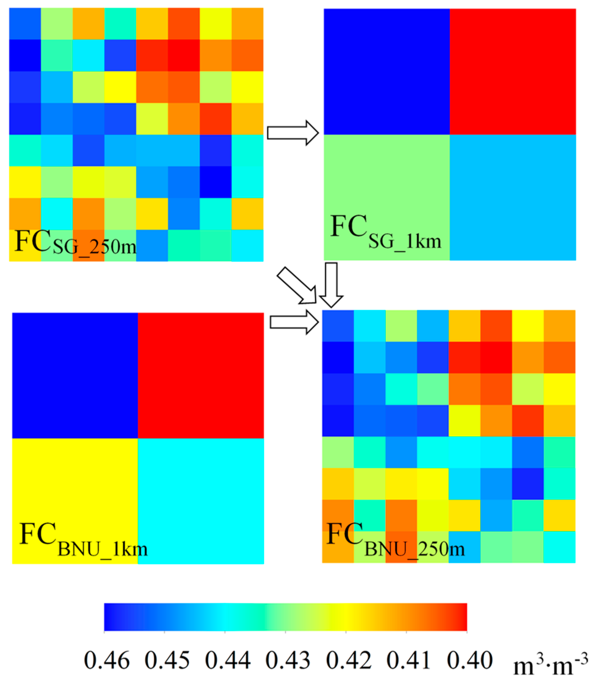
Although resampled to 250 m benchmark grids, the effective resolution of the FAO and BNU datasets was still 10 km and 1 km, respectively. As a result, the resolution of the ensemble members that were calculated based on the FAO and SG datasets were 10 km and 1 km, respectively. In order to matchup each ensemble member to a consistent scale, the SG-based field capacity ensemble member was used to downscale the FAO-/BNU-based field capacity ensemble members [47]. Figure 4 shows the scale matching process for two datasets of different resolutions. On considering a BNU-based ensemble member as an example, for a specific FC_{BNU_1km} grid, first we calculated the average values of FC_{SG_250m} within the grid, and then estimated FC_{BNU_250m} using Equation (6):

$$F{C}_{BNU\_250\mathrm{m}}=F{C}_{SG\_250\mathrm{m}}\times F{C}_{BNU\_1\mathrm{km}}/F{C}_{SG\_1\mathrm{km}}$$

(6)

The downscale algorithm only changed the distribution of the field capacity in the grid and kept the average values consistent.

2.2.4. Simulation in Desert Regions

For desert regions, such as the Taklamakan in south Xinjiang, the ensemble algorithm was driven only based on the BNU and SG datasets owing to the missing values of the FAO dataset for such areas. Furthermore, the sand content in the desert areas was higher than that in other areas, and there was no in situ station in these areas. Thus, it would be unreasonable to estimate the field capacity in desert areas using an ensemble formula established using samples of other soil types. We therefore extracted the desert areas using Maryland (UMD) landcover data [48] and selected a PTF [41] that was most suitable to simulate the field capacity of a desert based on the SG and BNU datasets (refer to the previous field capacity studies for desert areas). Finally, the integration approach was used to map the field capacity for the desert areas.

2.2.5. Validation Methods of Ensemble Field Capacity

Except for station-based validation, to further illustrate the simulation capability of the ensemble field capacity at the regional scale, we divided the whole of China into 217 soil units to evaluate its applicability. The 217 soil units were divided based on 14 climate sub regions, 139 geomorphology sub regions, and 64 soil type sub regions [49]. The climate, geomorphology, and soil type in a specific soil unit are relatively consistent, and therefore the field capacity within each unit would be close as well. For each soil unit, the mean values of the in situ field capacity and grid ensemble field capacity were calculated.

Further, to improve the reliability of the ensemble field capacity, comparison with BNU field capacity was also carried out. The field capacity in the BNU datasets was estimated using the median of ten established PTFs. The 250 m gridded ensemble field capacity was first upscaled to the BNU 1-km grids using the area-weighted average. We then calculated three statistical indicators, i.e., R, bias, and RMSE between ensemble field capacity and BNU field capacity.

3. Results

3.1. Distribution of Ensemble Field Capacity and Station Validation

Table 2. Evaluation statistical indicators for 24 groups of ensemble members. Bold text indicates the best behavior among each dataset. MLR represents multiple linear regression field capacity.

Datasets	Indicators	PTF1	PTF2	PTF3	PTF4	PTF5	PTF6	PTF7	MLR
FAO	σ	0.038	0.015	0.051	0.039	0.036	0.041	0.046	0.018
	Mean	0.273	0.323	0.344	0.300	0.330	0.302	0.306	0.357
	CV	0.138	0.045	0.148	0.131	0.110	0.137	0.151	0.052
	R	0.219	0.211	0.178	0.199	0.219	0.126	0.198	0.236
	RMSE	0.113	0.082	0.085	0.096	0.081	0.098	0.095	0.075
BNU	σ	0.047	0.032	0.066	0.049	0.051	0.069	0.057	0.020
	Mean	0.221	0.277	0.343	0.277	0.274	0.304	0.273	0.354
	CV	0.214	0.116	0.193	0.176	0.186	0.227	0.208	0.055
	R	0.201	0.210	0.159	0.183	0.196	0.155	0.192	0.258
	RMSE	0.157	0.110	0.094	0.114	0.116	0.108	0.119	0.074
SG	σ	0.024	0.015	0.032	0.022	0.027	0.031	0.024	0.025
	Mean	0.239	0.297	0.386	0.290	0.297	0.323	0.295	0.356
	CV	0.102	0.052	0.082	0.077	0.090	0.095	0.081	0.069
	R	0.279	0.256	0.255	0.309	0.278	0.290	0.321	0.320
	RMSE	0.137	0.094	0.081	0.098	0.094	0.081	0.094	0.073

shows the σ, mean, CV, and R values between the in situ field capacity and ensemble members. In general, from among the three datasets, the best simulation result was obtained for the SG dataset with an average R of 0.289 (p < 0.001). In particular, the MLR was the best one among the eight PTFs for both FAO, SG, and BNU datasets. The σ, mean, and CV values of the in situ field capacity were 0.08, 0.36 m³∙m⁻³, and 0.22, respectively. All the 24 ensemble members had a lower σ than the in situ field capacity, indicating the weakness of these PTFs in simulating high and low field capacities. Except for the MLR equation of each dataset, almost every PTF had lower mean values than the in situ field capacity, thus demonstrating the system’s bias in applying these existing PTFs which were developed based on soil samples collected outside of China. The R for the SG dataset was remarkably higher than those of the FAO and BNU datasets. This was probably due to the lowest representative error of the SG dataset among the three datasets and the scale effect in the matching of these soil datasets with the in situ stations, considering the SG dataset had the highest spatial resolution among the three datasets.

The details of the three MLR equations are shown as follows.

FAO_MLR:	$\begin{array}{ll}fc=& -0.3294+0.0077\times sand+0.0091\times clay+0.0067\times silt+0.0066\times SOM-\\ & 0.0715\times BD\end{array}$
BNU_MLR:	$fc=-0.0513+0.0017\times clay-0.00003\times silt+0.0088\times SOM+0.1926\times BD$
SG_MLR:	$\begin{array}{ll}fc=& -0.5287-0.0043\times sand+0.0003\times clay-0.0022\times silt+0.0026\times SOM+\\ & 0.0235\times BD\end{array}$

After operating the algorithm, we selected FAO_MLR, BNU_MLR, and SG_MLR as the optimal combination of ensemble members. The R and RMSE between ensemble field capacity and in situ field capacity were 0.37 and 0.073 m³·m⁻³, respectively. Thus, the R and RMSE performances had been improved compared with a single ensemble member.

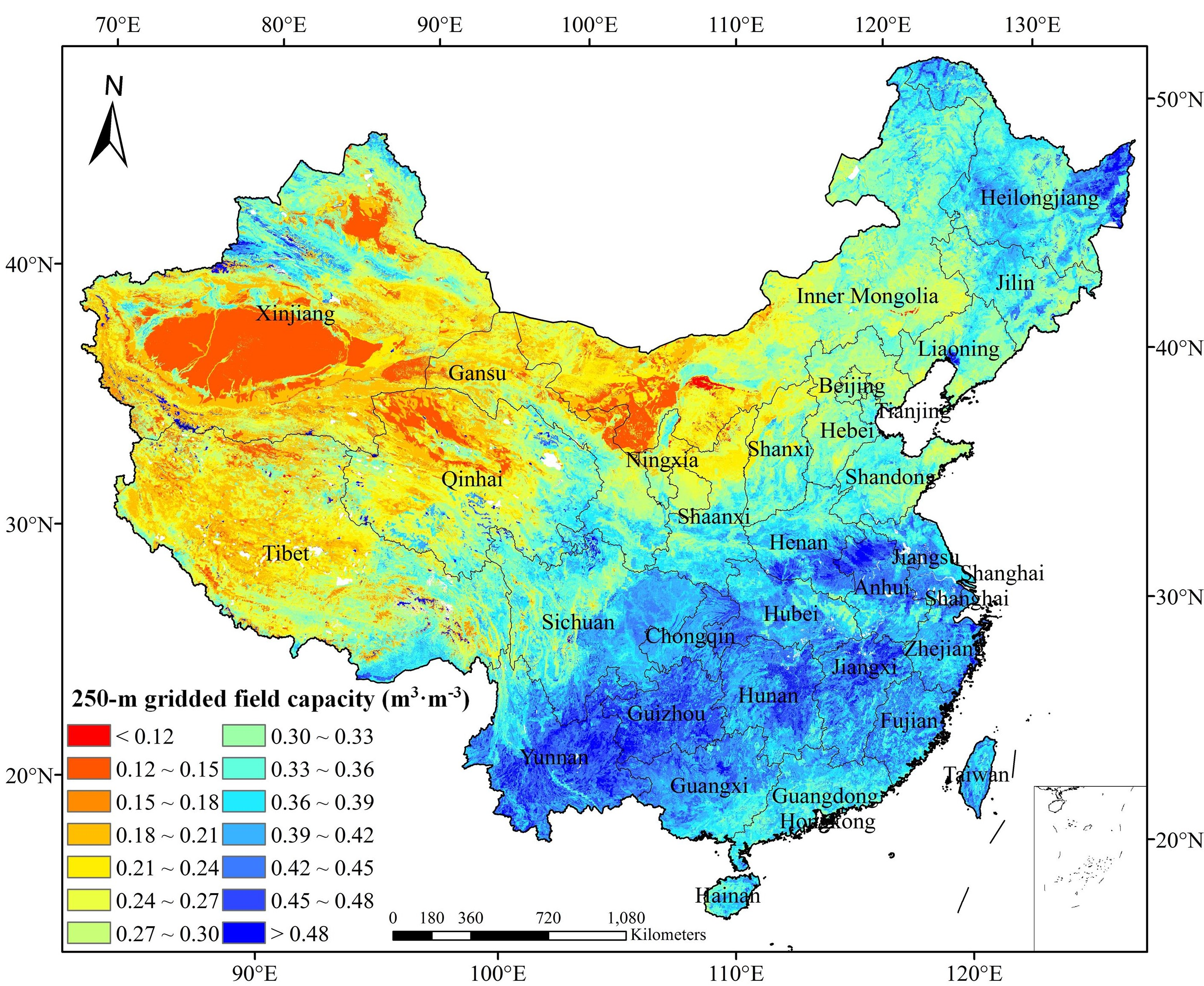
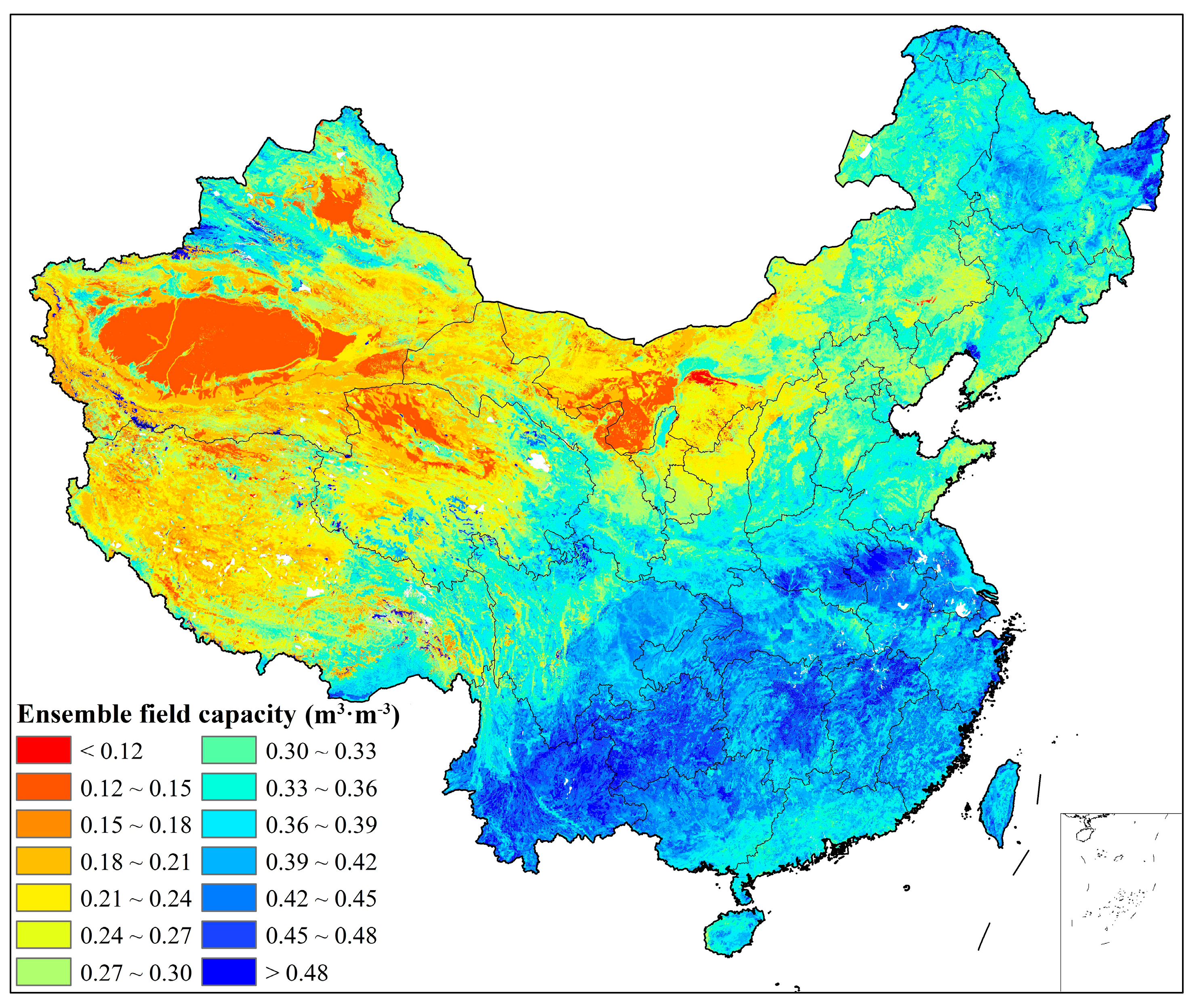
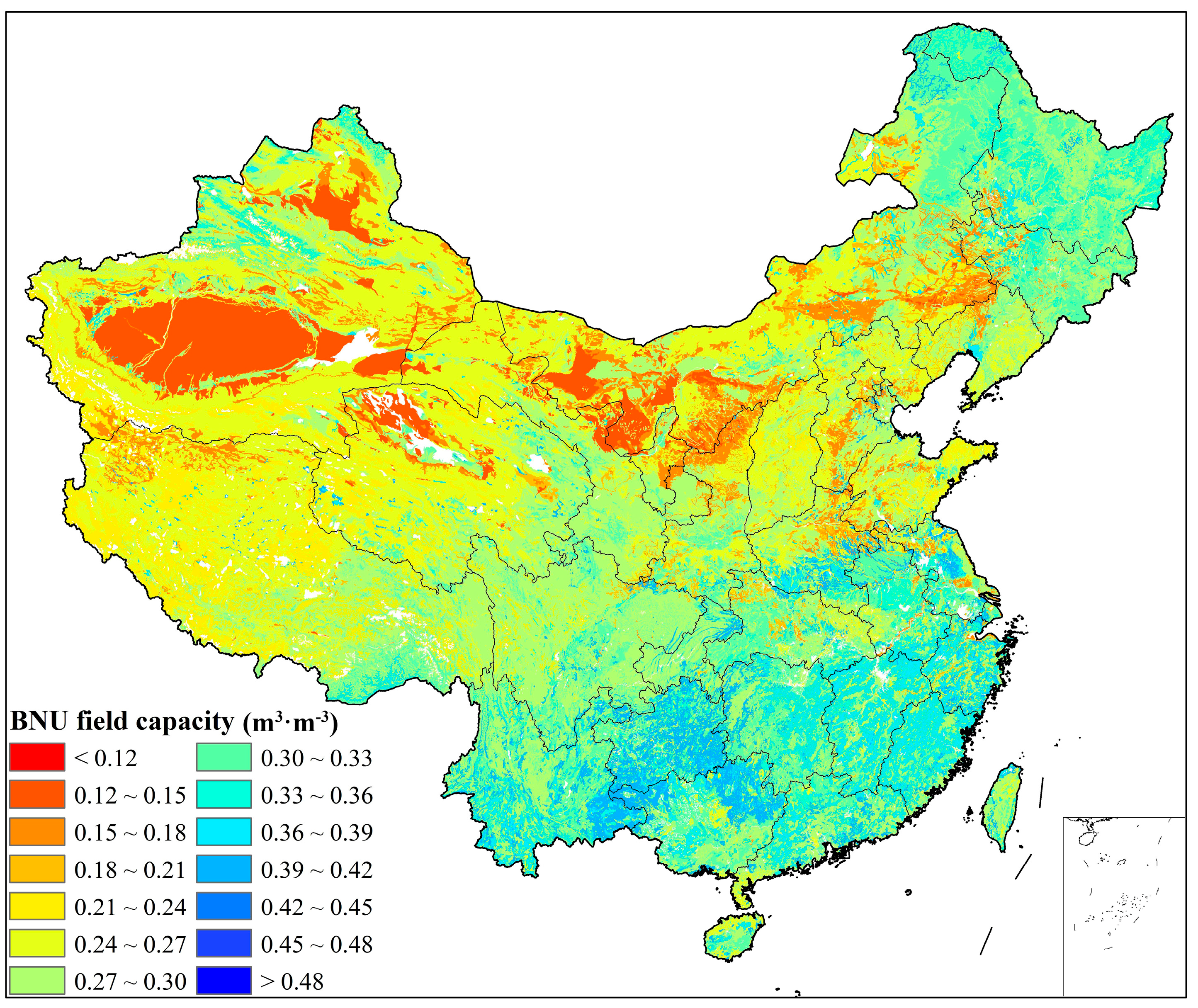
Figure 5 shows the distribution of the field capacity mapped using the integration approach. The minimum value of the ensemble field capacity was 0.08 m³·m⁻³, which was found in the Taklamakan (southern Xinjiang province) and Alashan (northern Gansu province) desert areas. The maximum value of the ensemble field capacity was 0.60 m³·m⁻³, which was found in the Yangtze River basin in southwestern China and the eastern Heilongjiang province. The average ensemble field capacity was 0.31 m³∙m⁻³, which was slightly less than the mean value of the in situ field capacity (owing to the missing values of the low field capacity areas, e.g., the Tibet Plateau). The field capacity map illustrated that the field capacity values in north China were generally below 0.36 m³∙m⁻³ (expect in the Heilongjiang province owing to it being rich in forest resources and black soil). The field capacity values increased gradually from northwest to southeast, and they were generally greater than 0.40 m³∙m⁻³ in South China.

Figure 6 shows the in situ field capacity. Figure 5 and Figure 6 show great consistency in field capacity distribution. The regions that have maximum and minimum field capacities were very close, and the spatial distribution tendency of these two sets of field capacities were quite similar. However, there was a clear difference between the two maps in the southern Henan and southern Hebei province. The reasons contributing to this difference may include the following two aspects: One possible reason was the measurement error in the in situ field capacity in this region, which results in the in situ field capacity being generally higher than the true field capacity. Further field experiment is needed to determine whether it is true. The error may have also come from the regression model itself for incomplete generalization of effect factors. For example, there were other dominant factors that impacted the field capacity in this region, i.e., long-term irrigation or human activities, which influenced the accuracy of the PTFs suitability in a specific region.

3.2. Validation of Ensemble Field Capacity at the Regional Scale

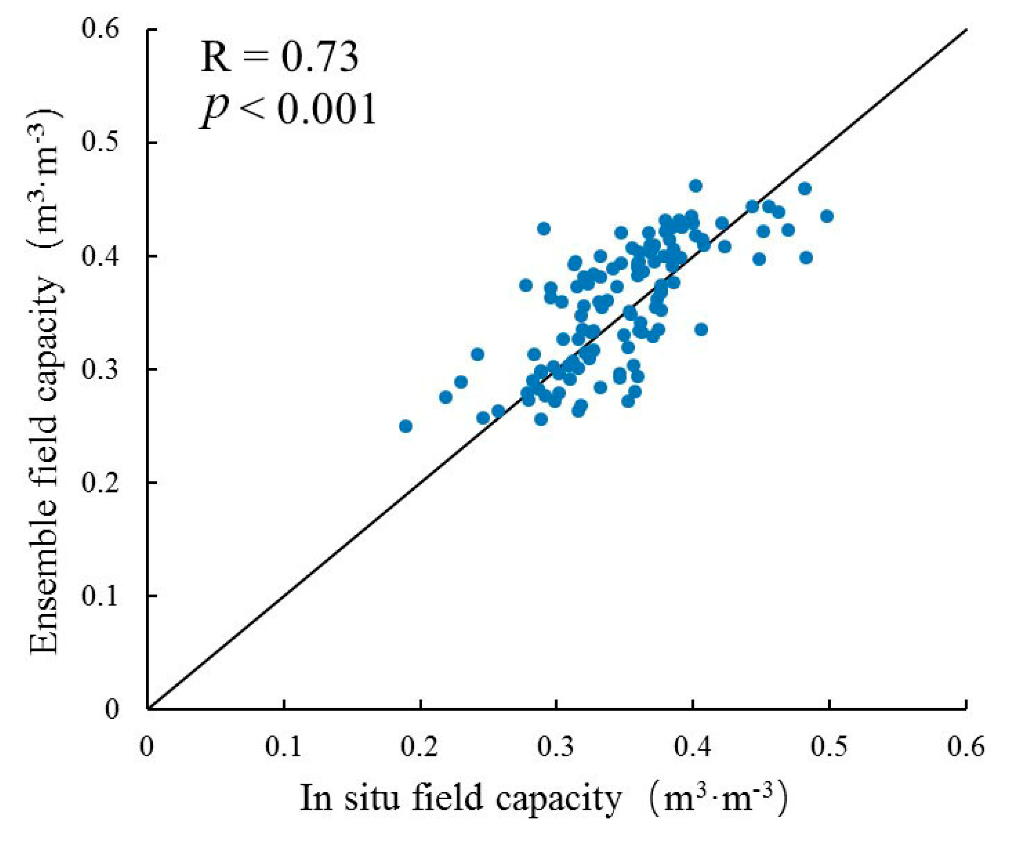
Figure 7 shows the scatterplot of the mean in situ field capacity and ensemble field capacity in 217 soil units. The R and RMSE between these two field capacities were 0.73 (n = 133 and p < 0.001) and 0.048 m³∙m⁻³, respectively, which demonstrates that the ensemble field capacity was simulated well at regional scale. Among these soil units, over 75% of the bias between the two mean field capacities was less than 0.05 m³∙m⁻³, while over 50% of the bias was less than 0.025 m³∙m⁻³.

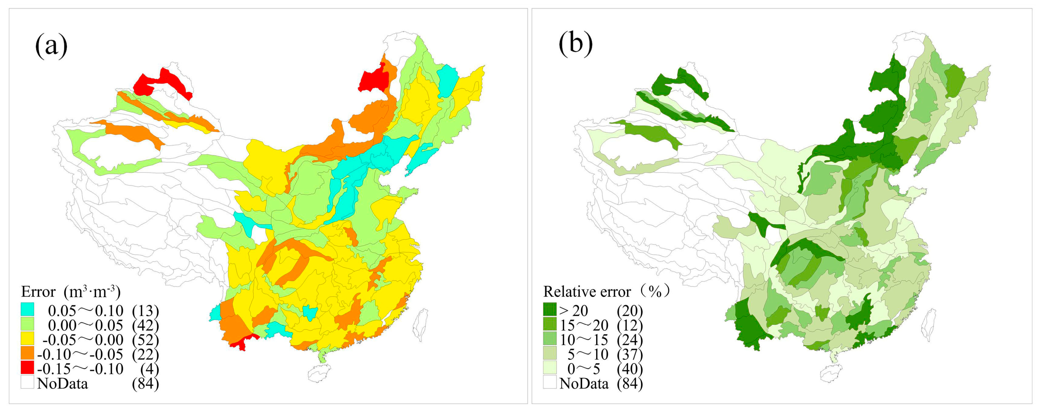
Figure 8a shows the distribution of the error between the in situ field capacity and ensemble field capacity at the regional scale (217 sub regions totally), wherein the error was calculated by subtracting ensemble field capacity from in situ field capacity. The error distribution showed an obvious regional regularity with the Yangtze River basin being the boundary, and the ensemble field capacity was generally greater than the in situ field capacity in the area south of the boundary. The error distributed north of the boundary was more complicated than that south of the boundary. A majority of the areas had an ensemble field capacity lower than the in situ field capacity, except in the cases of central Heilongjiang, Inner Mongolia, and north Xinjiang provinces. The maximum error appeared in the Shanxi, Hebei, and Liaoning provinces. The maximum negative error appeared in north Inner Mongolia, southwest Yunnan, and north Xinjiang provinces. Central and eastern China would be the most suitable for using the ensemble field capacity as they exhibited the lowest error from the whole of China.

Figure 8b shows the distribution of the relative error between the in situ and ensemble field capacities. The relative error of the majority of the soil units was less than 10%. This shows that the northeast Inner Mongolia, north Xinjiang, and southwest Yunnan provinces had the highest relative error among all the soil units, the values of which were greater than 20%. The relative error in the Jiangsu, Anhui, and Gansu provinces were the lowest with their values being less than 5%, which is acceptable for hydrology studies [50].

The reasons that contribute to the error distribution may be multi-aspects. From the model aspect, when the field capacity in a region was close to the average in situ field capacity of China, the simulation effect will be improved in theory. And it may also be affected by the distribution of soil properties and representative error of in situ stations. In brief, the error will be greater if the field capacity in a region varies greatly and the number of in situ stations is less. For example, in northeastern Inner Mongolia and northern Xinjiang provinces, low density and high heterogeneity of station field capacity may bring more error.

3.3. Comparison with BNU Field Capacity

Other than the physical and chemical properties, the BNU China soil datasets also provided soil hydraulic parameters, e.g., field capacity and hydraulic conductivity. Three statistical indicators (R, bias, and RMSE) between ensemble field capacity and BNU field capacity were calculated. The results show that the R values was 0.745, average bias was 0.039 m³∙m⁻³ (BNU field capacity was lower), and RMSE was 0.0739 m³∙m⁻³. Figure 9 shows the distribution of the BNU field capacity. The spatial trends in Figure 9 were similar to those in Figure 5. The ensemble and BNU field capacities in Southwest China, Jiangxi province, Hunan province, and north Anhui province were both relatively high, while those in the Qinghai-Tibet Plateau, Loess Plateau, and Gansu province were both lower than the other regions except in the case of the desert regions. However, there were significant differences (the BNU field capacity was lower) between the two field capacities in some regions such as the Hebei province. In order to figure out the reasons for this difference, examination of the BNU soil physical properties datasets revealed that BNU had higher sand content than other two datasets in Hebei province. The average sand contents of SG, FAO, and BNU were 35.4%, 36.8%, and 44.5%, respectively. Soil profiles from the second national soil survey (http://vdb3.soil.csdb.cn/extend/jsp/introduction) showed that the main soil composition in Hebei province were cinnamon soil, moisture soil, and brown soil, and the sand content in these soils were both not very high. The maximum sand content of SG, FAO, and BNU in Hebei province was 50%, 53%, and 83%, respectively. However, in BNU dataset, 14% of the grid had more than 70% sand content. Thus, the field capacity estimated using the BNU soil datasets in this region was significantly lower than the ensemble field capacity. This also indicated the importance of using multi-source soil datasets to reduce uncertainty.

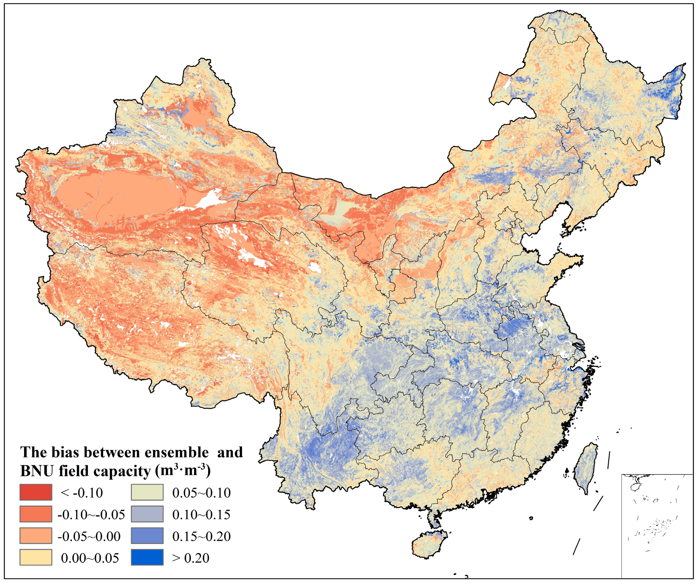
Figure 10 shows the bias between the ensemble field capacity and BNU field capacity. Except in the case of the north Qinghai-Tibet Plateau, west Inner Mongolia and south Xinjiang province, the ensemble field capacity was higher than the BNU field capacity in most regions of China. The highest bias was observed in the east Heilongjiang province, southwest China, and central China, where the field capacity was high. We first compared the basic soil datasets of SG and BNU. The overall distribution trends of these two datasets were similar, and the relative errors of sand, clay, silt, SOM, and BD between SG and BNU datasets were 0.12, 0.13, 0.15, 0.10, and 0.05, respectively. It was observed that the overall distribution trends on a large scale of these two datasets were similar. Considering that the BNU field capacity was calculated using PTFs trained by foreign soil samples, it was assumed that the specific regional climatic characteristics and soil characteristics in these regions caused the inapplicability of these PTFs.

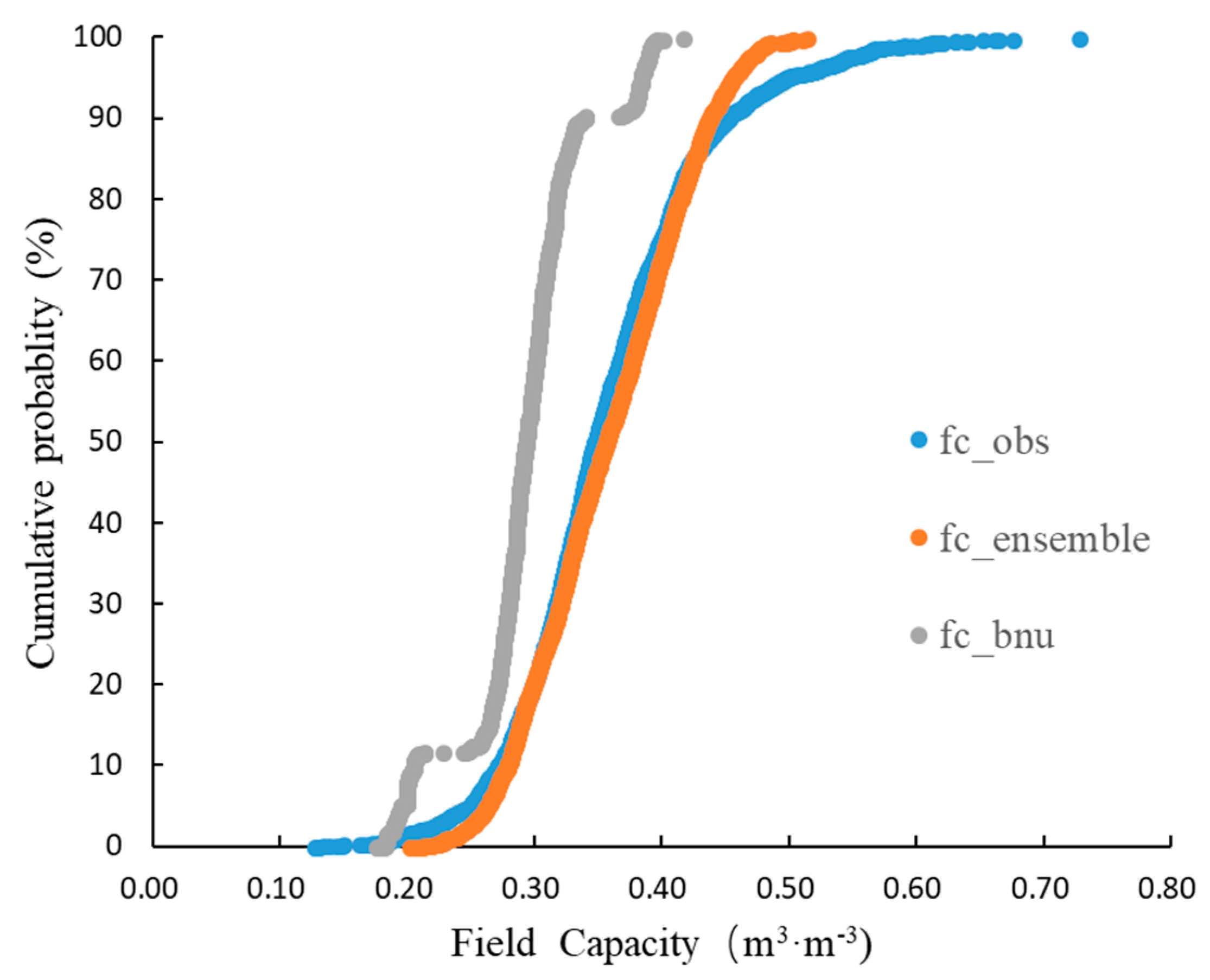
Figure 11 shows the cumulative distribution function of the in situ, ensemble, and BNU field capacity. The cumulative distribution curve of in situ field capacity was continuous and close to the normal distribution, which was consistent with Wang’s research result [51]. It demonstrates that the ensemble field capacity between 0.30–0.45 m³∙m⁻³ had same cumulative probability curve as the in situ field capacity. When the field capacity was greater than 0.45 m³∙m⁻³ or less than 0.30 m³∙m⁻³, the simulation effect will be relatively insufficient. This also demonstrated that more effort should be focused on estimating high/low values of field capacity. However, the BNU field capacity was lower than the other two field capacity, and the BNU FC curve was discontinuous at 10 and 88 cumulative probability (%), which was not reasonable in a field capacity cumulative distribution function. Compared with the BNU FC curve, in situ FC, and ensemble FC curves were closer to the normal distribution.

4. Discussion

As mentioned above, only one ensemble formula was used to map the field capacity over China. To evaluate the accuracy and reliability of the ensemble field capacity in a specific small region, some comparisons with previous studies were made. The core purpose of the comparisons was to compare the consistency in spatial distribution and analyze the reasons that contribute to the discrepancy in the mapped field capacity between the various methods.

Table 3. Summary of regional validation. The specific location information of these four places can be found in Figure 1.

Researcher	Region	Field Capacity Mapping Method	Field Capacity Distribution Trend	Validation with Ensemble Field Capacity
Wang [51]	Loess Plateau	Geostatistical method	Reduces from southeast to northwest	Consistent with Spatial trend and quantity
Yang et al. [52]	North and northeast China	AMSR-E-based model	Highest in north Henan	Consistent with spatial trend, different in quantity
Zhang [53]	Shaanxi	Qualitative and quantitative analysis	Fluctuating change from south to north	Consistent with spatial trend and quantity
Wang et al. [54]	Middle Heilongjiang	PTFs based on HWSD	Decreases from west to east	Overall similar, different in part of the area

summarizes the results of the regional validation.

Overall, the ensemble field capacity was similar considering the distribution of field capacity with their studies, however, there were some differences in the quantity. Yang et al. [52] counted the maximum values for each grid in the North China Plain and in northeast China using Advanced Microwave Scanning Radiometer-EOS (AMSR-E) soil moisture product from 2003 to 2007 and estimated the field capacity using soil moisture one day after the counted date. The overall field capacity values of Yang’s research were lower than the ensemble field capacity values. We suppose that there may be two reasons for this. One reason is that the observation depth of the AMSR-E was not sufficient. The second reason is that it was difficult for the soil moisture in this region to reach the maximum values in the period of 2003 to 2007, which resulted in lower values when the field capacity was estimated using this method. Wang et al. [54] estimated the 1 km gridded field capacity in the Hulan River basin, Heilongjiang province using PTFs established by Duan et al. [55] based on the HWSD, and there was an apparent difference in the middle of the basin, which may be caused by different PTFs or soil datasets.

Moreover, the integration approach proposed in this paper was flexible and extensible. On one hand, more accurate soil datasets could be added to the ensemble to enhance its robustness and reduce the uncertainty in the estimation of the field capacity. On the other hand, besides the PTFs and the regression equation, new modeling methods, e.g., a support vector machine (SVM), can also be used to improve the ensemble members [14,56]. Focusing on a specific small region as the study area in order to calibrate the parameters of the integration approach would help to improve the simulation capability.

The ensemble field capacity simulated well in gauged areas, and it also has the potential for application in ungauged areas. It is a product that has the potential for practical applications. However, there are still some uncertainties to be solved: (1) The representativeness error due to the scale problem includes various spatial resolutions of the three soil datasets and the scale mismatch in determining the station soil properties; (2) the vertical distribution of the field capacity. In this paper, we only calculated the average field capacity for a soil depth of 0–40 cm while simulating the vertical distribution and extending the field capacity to the root-zone area is still a problem; and (3) more soil properties or human activities can be considered in the integration approach.

5. Conclusions

In this paper, 2388 in situ field capacity data from 2388 sites in China were collected to develop an integration approach for mapping a 250 m gridded field capacity distribution. The obtained results are summarized as follows:

(1)

The accuracy and applicability of the existing PTFs based on the FAO, BNU, and SG soil datasets were analyzed in China. The results demonstrate the relatively unreliable performance of these PTFs or products. Almost all of them underestimated the field capacity with the average bias between 0.02 to 0.10 m³∙m⁻³.

(2)

An integration approach was proposed for estimating the 250 m gridded field capacity based on the field capacities of 2388 in situ stations and multi-source soil datasets. Three soil datasets were used to determine 24 ensemble members; after the algorithm progress, three best ensemble members were selected and included into the ensemble formula to obtain the ensemble field capacity at 250 m grids in China.

(3)

The ensemble field capacity was validated using in situ data and existing field capacity products. The validation result demonstrated that the ensemble field capacity had identical spatial characteristics with that of the in situ data and other products, and it can be used to revise the systematic error in the BNU field capacity and existing PTFs in China. It is a potential field capacity product for future practical applications.

References

- Sanchez, P.A.; Ahamed, S.; Carré, F.; Hartemink, A.E.; Hempel, J.; Huising, J.; Lagacherie, P.; Mcbratney, A.B.; Mckenzie, N.J.; Mendonça-Santos, M.D.L.; et al. Digital Soil Map of the World. Science 2009, 325, 680–681. [Google Scholar] [CrossRef] [PubMed]
- Piedallu, C.; Gégout, J.C.; Bruand, A.; Seynave, I. Mapping soil water holding capacity over large areas to predict potential production of forest stands. Geoderma 2011, 160, 355–366. [Google Scholar] [CrossRef] [Green Version]
- Filho, T.B.O.; Leal, I.F.; Macedo, J.R.D.; Reis, B.C.B. An Algebraic Pedotransfer Function to Calculate Standardized in situ Determined Field Capacity. J. Agric. Sci. 2016, 8, 158. [Google Scholar] [CrossRef]
- Cassel, D.K.; Nielsen, D.R.; Klute, A. Methods of Soil Analysis; American Society of Agronomy: Madison, WI, USA, 1986; pp. 901–926. [Google Scholar]
- Martínez-Fernández, J.; González-Zamora, A.; Sánchez, N.; Gumuzzio, A. A soil water based index as a suitable agricultural drought indicator. J. Hydrol. 2015, 522, 265–273. [Google Scholar] [CrossRef]
- Markovic, M.; Filipovic, V.; Legovic, T.; Josipovic, M.; Tadic, V. Evaluation of different soil water potential by field capacity threshold in combination with a triggered irrigation module. Soil Water Res. 2015, 10, 164–171. [Google Scholar] [CrossRef]
- Cong, Z.T.; Lü, H.F.; Guang-Heng, N.I. A simplified dynamic method for field capacity estimation and its parameter analysis. Water Sci. Eng. 2014, 7, 351–362. [Google Scholar]
- Arslan, H.; Tasan, M.; Yildirim, D.; Koksal, E.S.; Cemek, B. Predicting field capacity, wilting point, and the other physical properties of soils using hyperspectral reflectance spectroscopy: Two different statistical approaches. Environ. Monit. Assess. 2014, 186, 5077–5088. [Google Scholar] [CrossRef] [PubMed]
- Twarakavi, N.K.C.; Sakai, M.; Šimůnek, J. An objective analysis of the dynamic nature of field capacity. Water Resour. Res. 2009, 45, 82–90. [Google Scholar] [CrossRef]
- Patil, N.G.; Singh, S.K. Pedotransfer Functions for Estimating Soil Hydraulic Properties: A Review. Pedosphere 2016, 26, 417–430. [Google Scholar] [CrossRef]
- Wösten, J.H.M.; Pachepsky, Y.A.; Rawls, W.J. Pedotransfer functions: Bridging the gap between available basic soil data and missing soil hydraulic characteristics. J. Hydrol. 2001, 251, 123–150. [Google Scholar] [CrossRef]
- Zhao, C.; Shao, M.A.; Jia, X.; Nasir, M.; Zhang, C. Using pedotransfer functions to estimate soil hydraulic conductivity in the Loess Plateau of China. Catena 2016, 143, 1–6. [Google Scholar] [CrossRef] [Green Version]
- Yi, X.; Li, G.; Yin, Y. Comparison of three methods to develop pedotransfer functions for the saturated water content and field water capacity in permafrost region. Cold Reg. Sci. Technol. 2013, 88, 10–16. [Google Scholar] [CrossRef]
- Ghorbani, M.A.; Shamshirband, S.; Haghi, D.Z.; Azani, A.; Bonakdari, H.; Ebtehaj, I. Application of firefly algorithm-based support vector machines for prediction of field capacity and permanent wilting point. Soil Tillage Res. 2017, 172, 32–38. [Google Scholar] [CrossRef]
- Haghverdi, A.; Cornelis, W.M.; Ghahraman, B. A pseudo-continuous neural network approach for developing water retention pedotransfer functions with limited data. J. Hydrol. 2012, 442–443, 46–54. [Google Scholar] [CrossRef]
- Aitkenhead, M.J.; Coull, M.C. Mapping soil carbon stocks across Scotland using a neural network model. Geoderma 2016, 262, 187–198. [Google Scholar] [CrossRef]
- Reynolds, C.A.; Jackson, T.J.; Rawls, W.J. Estimating soil water-holding capacities by linking the Food and Agriculture Organization Soil Map of the World with global pedon databases and continuous pedotransfer functions. Water Resour. Res. 2000, 36, 3653–3662. [Google Scholar] [CrossRef]
- Dai, Y.; Shangguan, W.; Duan, Q.; Liu, B.; Fu, S.; Niu, G. Development of a China Dataset of Soil Hydraulic Parameters Using Pedotransfer Functions for Land Surface Modeling. J. Hydrometeorol. 2013, 14, 869–887. [Google Scholar] [CrossRef]
- Sun, H.; Yang, J. Modified Numerical Approach to Estimate Field Capacity. J. Hydrol. Eng. 2013, 18, 431–438. [Google Scholar] [CrossRef]
- Saxton, K.E.; Rawls, W.J. Soil water characteristic estimates by texture and organic matter for hydrologic solutions. Soil Sci. Soc. Am. J. 2006, 70, 1569–1578. [Google Scholar] [CrossRef]
- Saxton, K.E.; Rawls, W.J.; Romberger, J.S.; Papendick, R.I. Estimating generalized soil-water characteristics from texture. Soil Sci. Soc. Am. J. 1986, 50, 1031–1036. [Google Scholar] [CrossRef]
- Li, Y.; Chen, D.; White, R.E.; Zhu, A.; Zhang, J. Estimating soil hydraulic properties of Fengqiu County soils in the North China Plain using pedo-transfer functions. Geoderma 2007, 138, 261–271. [Google Scholar] [CrossRef]
- Tóth, B.; Weynants, M.; Nemes, A.; Makó, A.; Bilas, G.; Tóth, G. New generation of hydraulic pedotransfer functions for Europe. Eur. J. Soil Sci. 2015, 66, 226–238. [Google Scholar] [CrossRef] [PubMed]
- Wösten, J.H.M.; Lilly, A.; Nemes, A.; Bas, C.L. Development and use of a database of hydraulic properties of European soils. Geoderma 1999, 90, 169–185. [Google Scholar] [CrossRef]
- Toth, Z. Ensemble forecasting at NMC: The generation of perturbations. Am. Meteorol. Soc. 1993, 74, 2317–2330. [Google Scholar] [CrossRef]
- Toth, Z.; Kalnay, E. Ensemble Forecasting at NCEP and the Breeding Method. Mon. Weather Rev. 1997, 125, 3297–3319. [Google Scholar] [CrossRef] [Green Version]
- Zhou, W.; Liu, G.; Pan, J.; Feng, X. Distribution of available soil water capacity in China. J. Geogr. Sci. 2005, 15, 3–12. [Google Scholar] [CrossRef]
- Zhang, J.; Lin, Z. Climate of China; Shanghai Scientific and Technical Publishers: Shanghai, China, 1992; pp. 301–304. [Google Scholar]
- Wang, S.; Mo, X.; Liu, S.; Lin, Z.; Hu, S. Validation and trend analysis of ECV soil moisture data on cropland in North China Plain during 1981–2010. Int. J. Appl. Earth Obs. Geoinf. 2016, 48, 110–121. [Google Scholar] [CrossRef] [Green Version]
- Hengl, T.; Mendes, D.J.J.; Heuvelink, G.B.; Ruiperez, G.M.; Kilibarda, M.; Blagotić, A.; Shangguan, W.; Wright, M.N.; Geng, X.; Bauermarschallinger, B. SoilGrids250m: Global gridded soil information based on machine learning. PLoS ONE 2017, 12, e169748. [Google Scholar] [CrossRef] [PubMed]
- Wrb, I.W.G. World Reference Base for Soil Resources. A Framework for International Classification, Correlation and Communication; World Soil Resources Reports; Food and Agriculture Organization: Rome, Italy, 2006. [Google Scholar]
- Batjes, N.H. Harmonized soil property values for broad-scale modelling (WISE30sec) with estimates of global soil carbon stocks. Geoderma 2016, 269, 61–68. [Google Scholar] [CrossRef]
- Nachtergaele, F.O.; Velthuizen, H.; Verelst, L.; Batjes, N.H.; Dijkshoorn, K.; Engelen, V.; Fischer, G.; Jones, A.; Montanarella, L. Harmonized World Soil Database, version 1.2; FAO: Rome, Italy; IIASA: Laxenburg, Austria, 2012. [Google Scholar]
- Shangguan, W.; Dai, Y.; Liu, B.; Ye, A.; Yuan, H. A soil particle-size distribution dataset for regional land and climate modelling in China. Geoderma 2012, 171–172, 85–91. [Google Scholar] [CrossRef]
- Shangguan, W.; Dai, Y.; Liu, B.; Zhu, A.; Duan, Q.; Wu, L.; Ji, D.; Ye, A.; Yuan, H.; Zhang, Q.; et al. A China data set of soil properties for land surface modeling. J. Adv. Model. Earth Syst. 2013, 5, 212–224. [Google Scholar] [CrossRef] [Green Version]
- Hu, G.; Jia, L. Monitoring of Evapotranspiration in a Semi-Arid Inland River Basin by Combining Microwave and Optical Remote Sensing Observations. Remote Sens. 2015, 7, 3056–3087. [Google Scholar] [CrossRef] [Green Version]
- Hengl, T.; de Jesus, J.M.; Macmillan, R.A.; Batjes, N.H.; Heuvelink, G.B.; Ribeiro, E.; Samuelrosa, A.; Kempen, B.; Leenaars, J.G.; Walsh, M.G.; et al. SoilGrids1km—Global Soil Information Based on Automated Mapping. PLoS ONE 2014, 9, e105992. [Google Scholar] [CrossRef] [PubMed]
- Leenaars, J.G.B.; Claessens, L.; Heuvelink, G.B.M.; Hengl, T.; González, M.R.; Bussel, L.G.J.V.; Guilpart, N.; Yang, H.; Cassman, K.G. Mapping rootable depth and root zone plant-available water holding capacity of the soil of sub-Saharan Africa. Geoderma 2018, 324, 18–36. [Google Scholar] [CrossRef]
- Mantel, S.; Caspari, T.; Kempen, B.; Schad, P.; Eberhardt, E.; Ruiperez Gonzalez, M. Evaluation of automated global mapping of Reference Soil Groups of WRB2015. In Proceedings of the 19th EGU General Assembly, Vienna, Austria, 23–28 April 2017; p. 16641. [Google Scholar]
- Global Soil Data Task. Available online: http://daac.ornl.gov/ (accessed on 6 April 2000).
- Bruand, A.; Baize, D.; Hardy, M. Prediction of water retention properties of clayey soils: Validity of relationships using a single soil characteristic. Soil Use Manag. 1994, 10, 99–103. [Google Scholar] [CrossRef]
- Canarache, A. Technological soil maps, a possible product of soil survey for direct use in agriculture. Soil Technol. 1993, 6, 3–15. [Google Scholar]
- Gupta, S.C.; Larson, W.E. Estimating soil water retention characteristics from particle size distribution, organic matter percent, and bulk density. Water Resour. Res. 1979, 15, 1633–1635. [Google Scholar] [CrossRef] [Green Version]
- Hall, D.G.M.; Reeve, M.J.; Thomasson, A.J.; Wright, V.F. Water Retention, Porosity and Density of Field Soils; Soil Survey Technical: Harpenden, UK, 1977; p. 75. [Google Scholar]
- Petersen, G.W.; Cunningham, R.L.; Matelski, R.P. Moisture Characteristics of Pennsylvania Soils: I. Moisture Retention as Related to Texture. Soil Sci. Soc. Am. J. 1968, 32, 271–275. [Google Scholar] [CrossRef]
- Tomasella, J.; Hodnett, M.G. Estimating soil water retention characteristics from limited data in Brazilian Amazonia. Soil Sci. 1998, 163, 190–202. [Google Scholar]
- Xu, C.Y. From GCMs to river flow: A review of downscaling methods and hydrologic modelling approaches. Prog. Phys. Geogr. 1999, 23, 229–249. [Google Scholar] [CrossRef]
- Hansen, M.; Defries, R.; Townshend, J.R.G.; Sohlberg, R. UMD Global Land Cover Classification, 1 Kilometer, 1.0; University of Maryland: College Park, MD, USA, 1998. [Google Scholar]
- Chen, X.; Ye, J.; Lu, G.; Qin, F. Study on field capacity distribution about soil of China. Water Resour. Hydropower Eng. 2004, 35, 113–119. [Google Scholar]
- Wei, H.; Shao, M.; Wang, Q.; Reichardt, K. Time stability of soil water storage measured by neutron probe and the effects of calibration procedures in a small watershed. Catena 2009, 79, 72–82. [Google Scholar]
- Wang, Y. Distribution and Influence Factors of Dried Soil Layers across the Loess Plateau. Ph.D. Thesis, Chinese Academy of Sciences, Shaanxi, China, 2010. [Google Scholar]
- Yang, S.; Wu, B.; Yan, N. Estimation of Soil Field Capacity in North China Plain and Northeast China Based on AMSR-E Data. Chin. J. Soil Sci. 2012, 43, 301–305. [Google Scholar]
- Zhang, K. Analysis of soil water holding capacity in Shaanxi province. Shaanxi Water Conserv. 2014, 2, 19–21. [Google Scholar]
- Wang, B.; Huang, J.; Gong, X. Grid Soil Moisture Constants Estimation based on HWSD over Basin. Hydrology 2015, 35, 8–11. [Google Scholar]
- Duan, Q.; Gupta, H.V.; Sorooshian, S.; Rousseau, A.N.; Turcotte, R. Use of a Priori Parameter Estimates in the Derivation of Spatially Consistent Parameter Sets of Rainfall-Runoff Models; American Geophysical Union: Washington, DC, USA, 2013; pp. 239–254. [Google Scholar]
- Khlosi, M.; Alhamdoosh, M.; Douaik, A.; Gabriels, D.; Cornelis, W.M. Enhanced pedotransfer functions with support vector machines to predict water retention of calcareous soil. Eur. J. Soil Sci. 2016, 67, 276–284. [Google Scholar] [CrossRef]
Figure 1.
Soil types map based on World Reference Base classification standard. The colorbar represents different soil types, and the names of the corresponding provinces are labelled.
Figure 2.
Overview of the study area and the distribution of in situ field capacity measurement stations.
Figure 3.
Algorithm for selecting field capacity ensemble members. FC represents field capacity.
Figure 4.
Scale matching for field capacity ensemble members. FCBNU_1km represents original BNU-based field capacity, FCSG_250m represents original SG-based field capacity, FCSG_1km represents upscaled mean values of FCSG_250m in corresponding grid, and FCBNU_250m represents downscaled field capacity based on BNU.
Figure 5.
Distribution of ensemble field capacity in China. Field capacity is mapped in a 250 × 250 m grid cell.
Figure 6.
Distribution of in situ field capacity in China. Color bar is same as that in Figure 5.
Figure 7.
Comparison of in situ field capacity and ensemble field capacity at the region scale. Here p values represent confidence interval. Soil units in which the number of stations was no more than two are excluded.
Figure 8.
Distribution of (a) error and (b) relative error between in situ field capacity and ensemble field capacity. Blank regions represent areas in which number of station was less than two. Numbers in parentheses represent the sum of corresponding regions. Error was calculated by subtracting ensemble field capacity from in situ field capacity.
Figure 9.
Distribution of BNU field capacity. Color bar is the same as that in Figure 5.
Figure 10.
Bias between ensemble field capacity and BNU field capacity. Bias was calculated by subtracting the BNU field capacity from ensemble field capacity.
Figure 11.
Cumulative distribution function of in situ, ensemble, and BNU field capacities. The fc_obs, fc_ensemble, and fc_bnu represent in situ, ensemble, and BNU field capacities, respectively.