Impacts of Climate Change on Soil Erosion in the Great Lakes Region

Abstract

Quantifying changes in potential soil erosion under projections of changing climate is important for the sustainable management of land resources, as soil loss estimates will be helpful in identifying areas susceptible to erosion, targeting future erosion control efforts, and/or conservation funding. Therefore, the macro-scale Variable Infiltration Capacity—Water Erosion Prediction Project (VIC-WEPP) soil erosion model was utilized to quantify soil losses under three climate change scenarios (A2, A1B, B1) using projections from three general circulation models (GFDL, PCM, HadCM3) for the Great Lakes region from 2000 to 2100. Soil loss was predicted to decrease throughout three future periods (2030s, 2060s, and 2090s) by 0.4–0.7 ton ha⁻¹ year⁻¹ (4.99–23.2%) relative to the historical period (2000s) with predicted air temperature increases of 0.68–4.34 °C and precipitation increases of 1.74–63.7 mm year⁻¹ (0.23–8.6%). In the forested northern study domain erosion kept increasing by 0.01–0.18 ton ha⁻¹ year⁻¹ over three future periods due to increased precipitation of 9.7–68.3 mm year⁻¹. The southern study domain covered by cropland and grassland had predicted soil loss decreases of 0.01–1.43 ton ha⁻¹ year⁻¹ due to air temperature increases of 1.75–4.79 °C and reduced precipitation in the summer. Fall and winter had greater risks of increased soil loss based on predictions for these two seasons under the A2 scenario, with the greatest cropland soil loss increase due to increased fall precipitation, and combined effects of increases in both precipitation and air temperature in the winter. Fall was identified with higher risks under the A1B scenario, while spring and summer were identified with the greatest risk of increased soil losses under the B1 scenario due to the increases in both precipitation and air temperature.

1. Introduction

It is critically important to clarify climate change impacts on soil loss to support the large-scale policies of land resource management and soil conservation in the U.S. Great Lakes region, which suffers from water quality degradation caused by agricultural nonpoint source pollution. Climate change studies of the Great Lakes region indicate projected increases in both precipitation and air temperatures [1,2,3]. By the end of the 21st century, annual precipitation is projected to increase up to 20% across the Great Lakes region [2] with precipitation increases in both winter and spring and decreases in summer [1,2]. Mean annual air temperature is projected to increase by 2.2 °C to 5.8 °C with more frequently occurring extreme heat events and more common heavy precipitation events [4,5,6].

Changes in air temperatures affect soil erosion processes through their influence on erosion driving factors: rates of runoff generation and soil infiltration [7,8,9,10,11]. Air temperature changes the soil evapotranspiration (ET) rate and soil moisture content, which in turn affects runoff generation and soil infiltration both of which control erosion processes [9,10]. Air temperature also changes the Leaf Area Index (LAI) of plants, which can change the soil’s exposure to precipitation and direct raindrop splash erosion processes. It can also affect biomass production and residue decomposition, which in turn may influence the infiltration and runoff processes [9,11]. Finally, increased air temperature changes cold season processes in the Midwest U.S. through increased snow melt and freeze-thaw cycles, and a decrease in the number of days with soil frost, which can increase soil loss in the winter and spring [12].

Changes in precipitation amount and patterns will influence the soil loss generation process by affecting runoff generation and rainfall erosivity. Increases in precipitation quantity will increase the probability of greater runoff generation, which in turn can increase soil loss under bare soil scenarios. Precipitation intensity and frequency are other factors increasing soil loss, as more than 50% of annual soil loss is caused by a few daily erosive events with high intensity [13,14]. Greater projected increases in rainfall intensities and storm energies will change the rainfall erosivity and create disparity in spatial trends between precipitation amount and rainfall erosivity [8]. Nearing et al. [15] conducted an investigation into the response of several different soil erosion models to changes in precipitation and land cover through a sensitivity analysis. They found that relative results from models were better than absolute predictions, and that soil erosion is more affected by changes in rainfall and canopy cover than runoff.

In a study by O’Neal et al. [11] with the Water Erosion Prediction Project (WEPP) [16,17] model, for 10 of 11 regions in the Midwestern U.S., runoff was projected to increase from 10% to 310%, and soil loss was projected to increase from 33% to 274% in 2040–2059 relative to 1990–1999. Increased precipitation and decreasing canopy cover from temperature-stressed maize were identified as important controlling factors. Zhang et al. [7] studied climate effects on runoff and soil erosion in southeastern Arizona rangelands for the 2050s and 2090s with the Rangeland Hydrology and Erosion Model (RHEM) [18] and found that while there were no significant changes in annual precipitation quantities across the region the projected mean annual runoff and soil loss increased significantly, ranging from 79% to 92% and from 127% to 157%, respectively, relative to 1970 to 1999. The increases in runoff and soil loss were attributed to the increase in the frequency and intensity of extreme events in the study area. Zhang and Nearing [19] studied climate change impacts on soil loss in central Oklahoma and found that annual precipitation was projected to decrease, while annual runoff and soil loss were projected to increase or be about the same by the latter part of this century depending on the future climate scenario. The increases in both soil loss and runoff were attributed to greater variability in monthly precipitation, which led to increased frequency of large storms.

Few papers have studied the climate change impacts on soil erosion in the Great Lakes region, much less take the spatial heterogeneity into consideration in clarification of future soil loss changes. Therefore, this paper studies the predicted runoff and soil loss changes under climate change impacts at annual and seasonal time steps as a result of projected changes in precipitation and air temperatures for the entire Great Lakes region and the three major land covers. A macro scale soil erosion model, the Variable Infiltration Capacity—Water Erosion Prediction Project (VIC-WEPP) model [20] was utilized in this study to estimate soil loss for the Great Lakes region in the historical period and in three future periods under three climate change scenarios.

2. Materials and Methods

2.1. Study Region

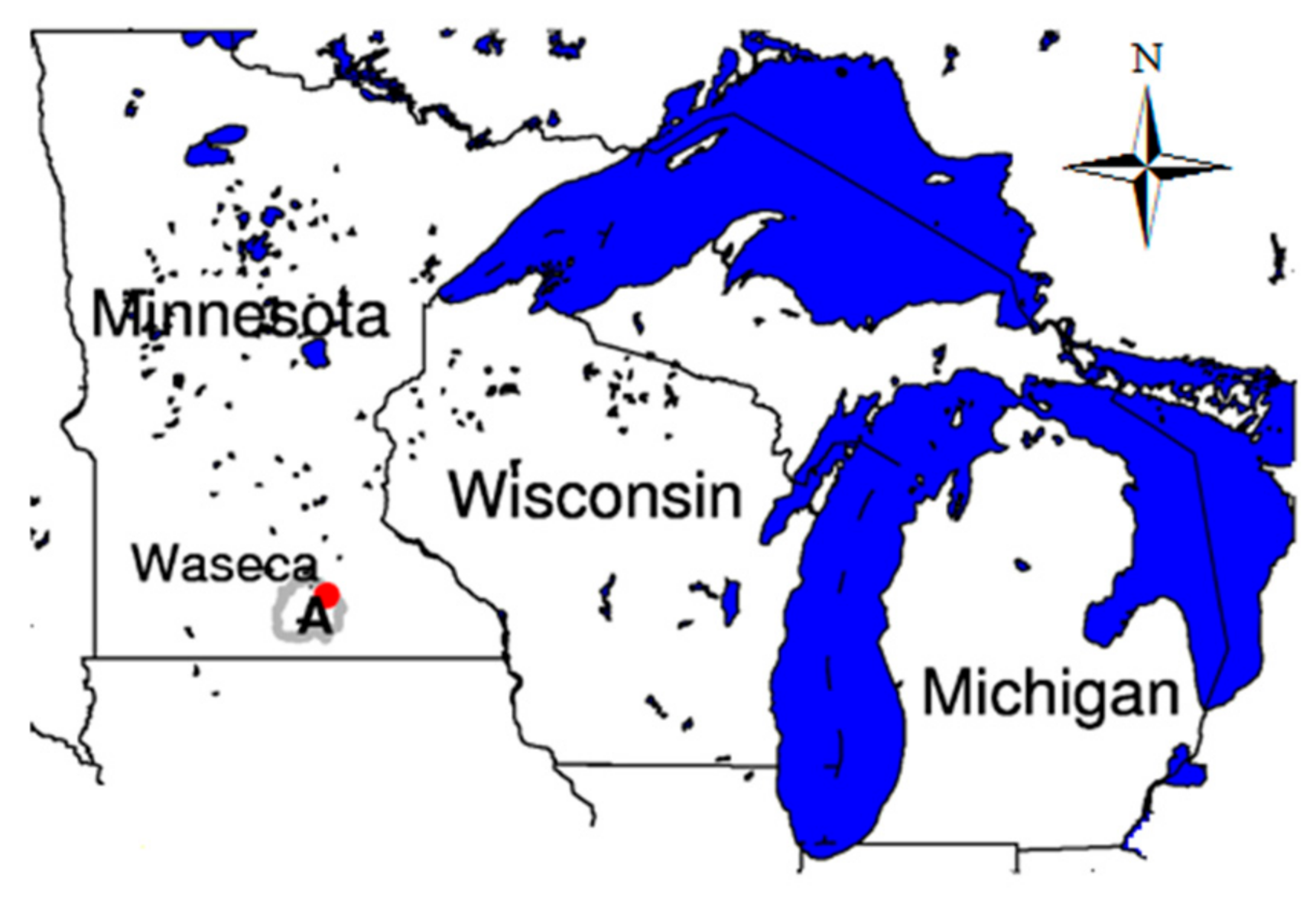
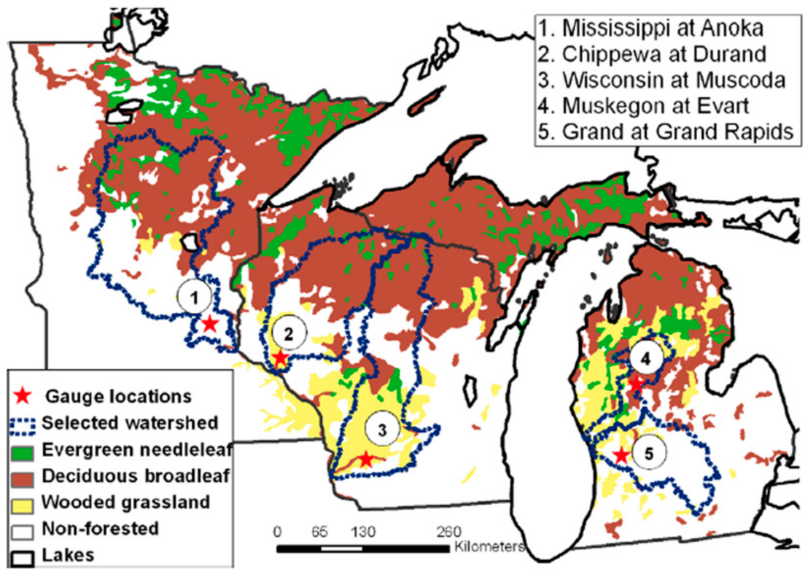
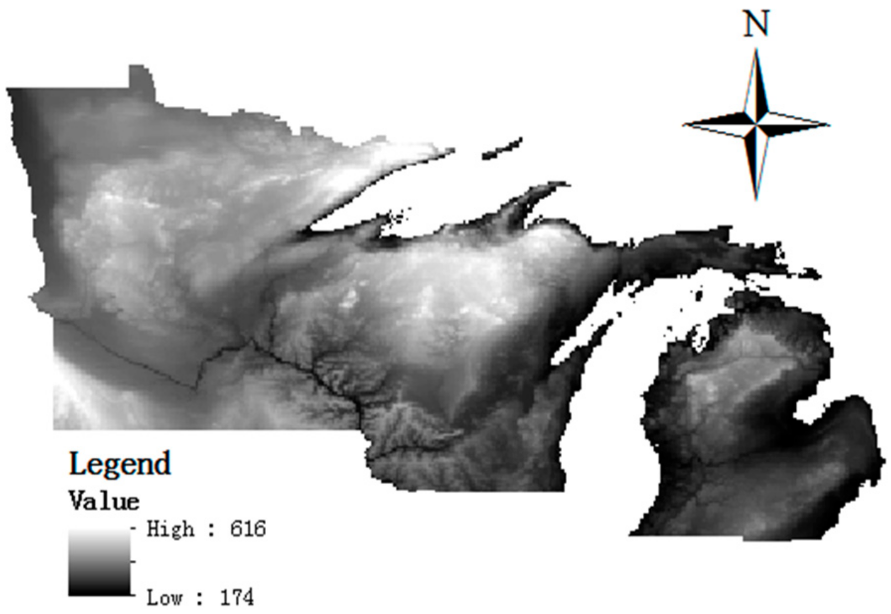
The study region covers three Great Lakes states: Wisconsin, Minnesota, and Michigan, with a total area of approximately 645,300 km² and a population of about 20 million (2010 U.S. census; Figure 1). It has a typical continental climate with a hot, wet summer and a cold, long winter, as the average summer precipitation is about 288 mm with air temperature of 20 °C, and winter precipitation is about 81 mm with an average air temperature around −8 °C. Annual average precipitation increases from western Minnesota (483 to 889 mm) to the eastern part of Michigan (762 to 1016 mm), with greater precipitation changes around the border between Wisconsin and Minnesota. Annual average temperatures increase gradually from the north border of Minnesota at about 2 °C to the south boundary of Michigan at about 10 °C. The study domain comprises parts of the upper Mississippi River basin (Wisconsin, Michigan), and parts of the Great Lakes drainage basin (Minnesota). 41% of the study domain is forest land, 9% is grassland, and 50% is cropland/non-forested area. The northern part of the study area is heavily forested with coniferous trees and broad leaf trees (Figure 2) [21]. The middle part is covered with grasses and the southern part is non-forested with agricultural land use in corn production [5,18]. The slopes of the study domain are flat except for those in the southern area, as the Mississippi Valley is located here with a high frequency of steep slopes (Figure 3).

2.2. Model Description

The coupled VIC-WEPP model is a macro scale soil erosion model, details of which can be found in Mao et al. [20]. For clarity, a brief introduction is provided here. The VIC-WEPP model is a coupled soil erosion model between the VIC model [21,22,23] and the WEPP-Hillslope Erosion (WEPP-HE) model [17,24,25]. This model can be used to estimate soil loss of grid cells with 1/8th degree latitude by longitude. In the VIC-WEPP model, WEPP-HE estimates soil loss of hill slopes within a grid cell based on the hydrologic parameters provided by VIC. The VIC-WEPP model was applied in this study instead of the WEPP model because the application scale of the VIC-WEPP model is much larger than the small agricultural fields which are appropriate for WEPP model utilization [24].

The VIC-WEPP model needs inputs of climate, slope, soil, and land cover for each grid cell within the study domain. Slope inputs were extracted from a 30 × 30 m DEM map downloaded from the U.S. seamless data server. Soil data was derived from the Conterminous United States Soil Characteristics Dataset [26] which is based on the State Soil Geographic Data Base (STATSGO) data and has been aggregated to the resolution of an eighth-degree grid cell. Land cover inputs were extracted from the land cover map in Mao and Cherkauer [27]. Cropland is dominated by corn (Zea mays) production and managed with fall chisel plow tillage method as it is the major operational tillage practice [18]. Soil loss was estimated for each one of the 4760 grid cells which composed the Great Lakes region.

2.3. General Circulation Models (GCMs) and Green House Gas (GHG) Scenarios

The climate dataset was from the Coupled Model Intercomparison Project 3 (CMIP3) datasets instead of the CMIP5 datasets [28], due to the inadequate representation of precipitation variability of the CMIP5 datasets in the Midwestern U.S. found by Wubble et al. [29] and the failure in capturing the increased intensity, duration and frequency of precipitation extremes described by Mohammed et al. [30] in the Champlain Basin. Three emission scenarios (A2, A1B, and B1) were selected based on the different characteristics of each scenario about the global economy, population, technology development, and energy consumption (the Special Report on Emission Scenarios SRES) [31]. The three GCMs were selected based on their sensitivity to GHG emissions from high to low. They were the GFDL-CM2 (Geophysical Fluid Dynamics Laboratory Version 1.1) [32,33], HADCM3 (Hadley Centre climate model Version 3.1) [34,35], and PCM (Parallel Climate Model Version 1.3) [36] models. The projected climate dataset from multiple model ensembles have been found to diminish spatial biases from individual GCMs [37].

Projected climate data was corrected and downscaled from monthly to daily data for each grid cell with the method of Wood et al. [38] and the support of historical Probability Density Functions (PDFs) from Sinha and Cherkauer [12]. In this study, the daily precipitation dataset from 2000 to 2099 was disaggregated into an hourly time step with the CLIGEN model (CLImate GENeration) [39] as soil erosion happens in a short time and near instantaneous rainfall intensity is important for infiltration excess runoff and soil erosion [40]. The historical period in this study is defined from 2000 to 2009, early century period is from 2030 to 2039, middle century period is from 2060 to 2069, and late century period is from 2090 to 2099.

2.4. Calibration and Validation

Calibration of the VIC-WEPP model in this study included two parts. The first part was the runoff calibration conducted by adjusting the hydrologic parameters in the VIC model. The second step was to assess soil loss estimates through comparison of the simulated and observed soil losses. Model streamflow calibration and evaluation of the Great Lakes region were conducted by Mao and Cherkauer [27] in five watersheds (Figure 2) which represent a large part of the study domain with satisfactory results for the Nash-Sutcliffe coefficient of efficiency [41] and the agreement index [42]. The calibrated model setting of streamflow by Mao and Cherkauer [27] was applied in this study. Soil loss calibration and validation of the VIC-WEPP model for the study domain was done through comparison between the simulated and observed soil losses of two sites (Waseca, MN and Morris, MN) by Mao et al. [20] with parameters obtained for the base inputs from the VIC model for each site.

2.5. Uncertainty Analysis

Model uncertainty analysis was performed in this study to make sure that the estimated soil loss of a grid cell was within the acceptable range with the clarified uncertainty. The General Likelihood Uncertainty Estimation (GLUE) approach [43] with Markov Chain Monte Carlo simulation was applied to quantify the VIC-WEPP model uncertainty in estimating soil loss at Waseca, MN (Figure 1). Monte Carlo sampling from a parameter space with normal distribution was done for five parameters of the VIC-WEPP model. The parameter Nash-Sutcliffe Efficiency (NSE) was used as the likelihood function with 0.5 as the threshold,

$$NSE=1-\frac{\sum {(Q_{obs}-Q_{sim})}^2}{\sum {(Q_{obs}-\overline{Q_{obs}})}^2}$$

(1)

where Q_obs is the observed value, Q_sim is the simulated value, $\overline{Q_{obs}}$ is the average observed value. The next three steps included calculation of likelihood values of behavioral parameter sets, rescaling these values to formulate a cumulative distribution, and derivation of quintiles of uncertainty from the cumulative distribution.

Climate change impacts on soil erosion were studied by analyzing the precipitation, air temperature, runoff, and soil loss changes between the historical period and the three future periods. To identify the areas susceptible to soil loss, the analysis was conducted for the entire study domain and the three major land covers over the three future periods under the three SRES scenarios. To identify the seasons with high risks of soil losses, the four parameters analysis was performed at annual and seasonal time steps in the three future periods (2030s, 2060s, 2090s) under the three SRES scenarios (A2, A1B, and B1) based on the characteristics of each scenario in the SRES report.

3. Results

3.1. Uncertainty Analysis of VIC-WEPP Model with GLUE Method

Though model calibration and validation is done in Mao and Cherkaur [27], to make sure the model reliability in estimating the soil loss, parameter uncertainty analysis is done in Waseca, IN with five parameters: the variable infiltration curve parameter, the maximum baseflow, fraction of dsmax where non-linear baseflow begins, fraction of the maximum soil moisture where non-linear baseflow occurs, and the saturated hydrologic conductivity. The five parameters are frequently used in the VIC model application studies to calibrate model for streamflow estimation [5,12,44] and used for VIC-WEPP model evaluation [27] about soil loss estimation. Parameters about soil erodibility and critical shear stress are calculated with the equations in WEPP-HE model based on the inputs from VIC model for the grid cell. Posterior distributions of the five parameters are obtained through analyzing the behavioral parameter sets and shown in

Table 1. Summary of posterior distribution for each parameter.

Statistics	Binf * (-)	Dsmax * (-)	Ds * (-)	Ws * (m m−1)	Ksat * (mm h−1)
Minimum	0.12	1.02	0	0.51	16.06
Maximum	0.40	35.50	0.93	1	29.52
Mean	0.30	1.31	0.10	0.85	23.82
Variance	0.01	69.56	0.04	0.02	15.88
Skewness	−0.50	3.05	2.14	−0.65	−0.21

* Note: B_inf denotes variable infiltration curve parameter; D_smax denotes maximum velocity of base flow; D_s denotes fraction of Dsmax where non-linear baseflow begins; W_s denotes fraction of maximum soil moisture where non-linear baseflow occurs; K_sat denotes saturated hydraulic conductivity.

. Three parameters about the variable infiltration curve parameter, the fraction of dsmax where non-linear baseflow begins, and the fraction of the maximum soil moisture where non-linear baseflow occurs are well identifiable parameters with less parameter uncertainty due to the small values of variances, while the rest two parameters with larger variance values indicate more scatter and larger parameter uncertainty.

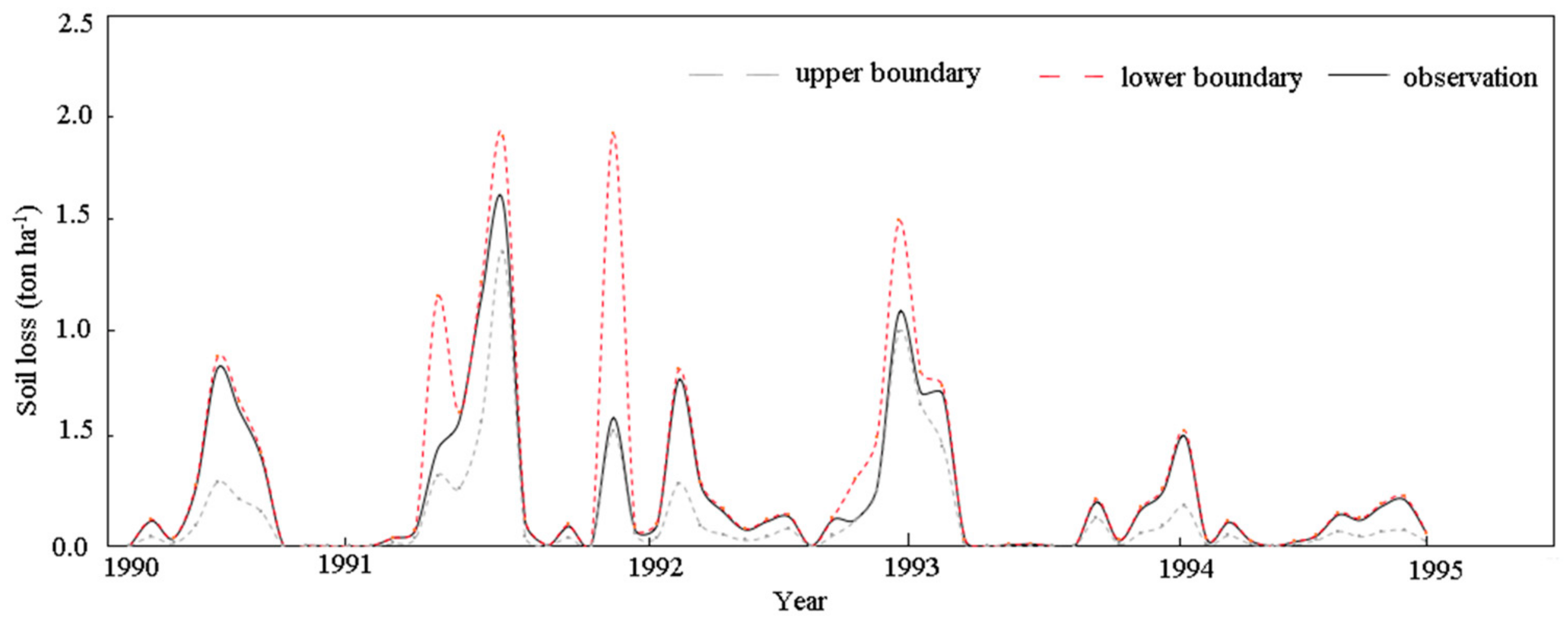
The GLUE method is applied to conduct a parameter uncertainty analysis using a threshold of NSE greater than or equal to 0.5 for the selection of behavioral parameter settings that ensure the model simulation effectiveness. The 95% confidence intervals are indicated in Figure 4 highlighted the uncertainty range caused by the parameters. The observed soil loss values are mostly within the 95% confidence intervals (Figure 4). The uncertainty is lower for the months with low soil loss quantity, while greater for months with great soil loss. The evaluation results demonstrate that the parameter settings for the VIC-WEPP model produce reasonable estimates of soil loss estimation in the grid cell of Waseca site, MN.

3.2. Analysis of Climate Change for the Great Lakes Region

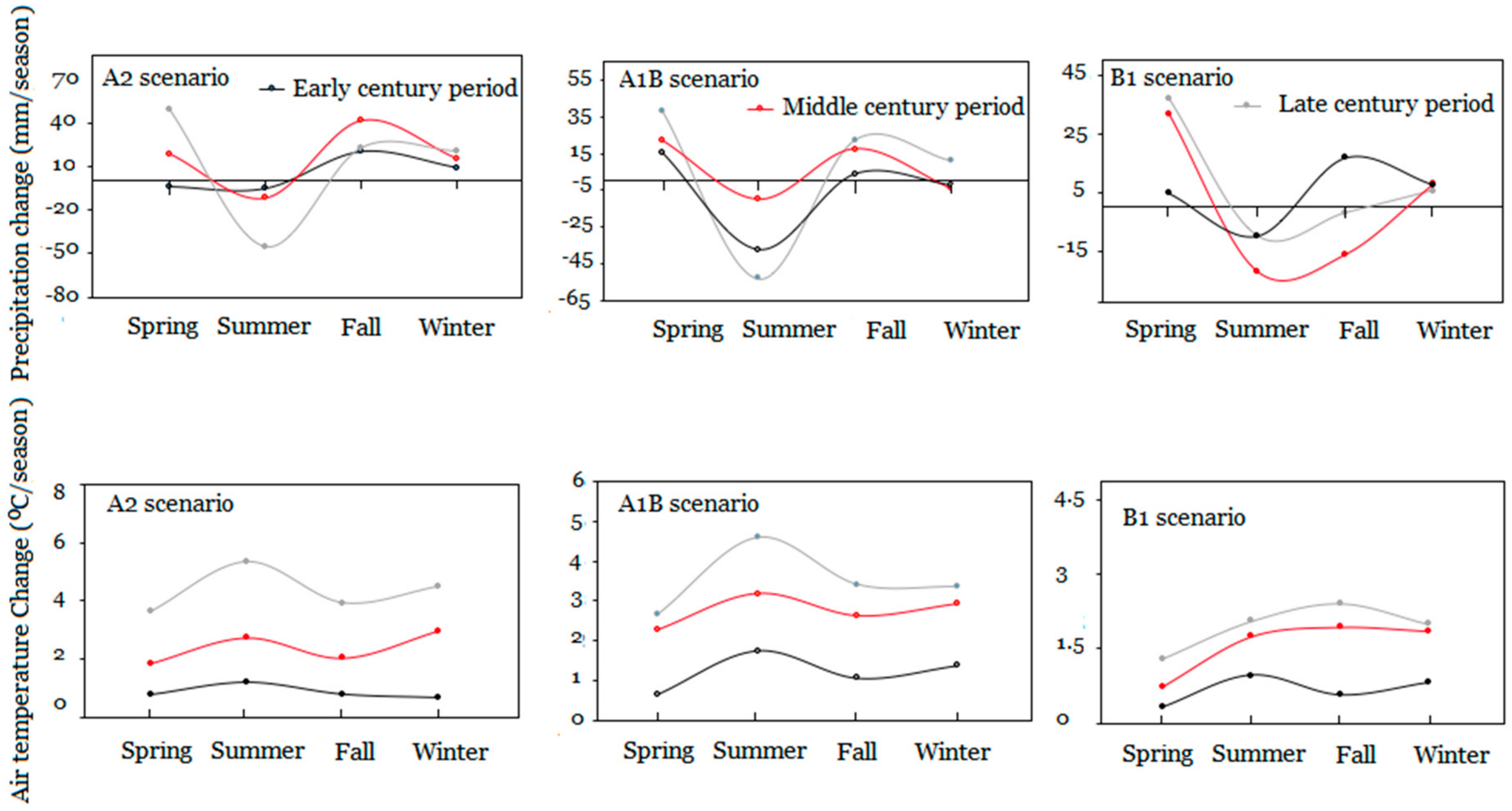
For the entire Great Lakes region, annual precipitation is projected to increase constantly by 1.74 (0.23%) to 63.71 mm (8.07%) over three future periods with the greatest increase in the middle century period under the A2 and A1B scenarios (

Table 2. Annual changes of precipitation and air temperature of the entire Great Lakes region over three future periods under three climate change scenarios.

Entire Region	A2			A1B			B1
	Early	Middle	Late	Early	Middle	Late	Early	Middle	Late
∆ Prec. (mm year−1)	20.11	63.71	47.42	20.71	25.41	18.72	19.01	1.74	30.80
%	2.55	8.07	6.01	2.61	3.21	2.36	2.51	0.23	4.12
∆ Temp. (°C)	0.85	2.39	4.34	1.47	2.76	3.52	0.68	1.57	1.94

, Figure 5). Spatially, croplands have the greatest increase of annual precipitation followed by the forest and grass areas (Figure S1,

Table 3. Annual changes of precipitation of three major land covers in three future periods under three SRES scenarios.

∆Prec. (mm Year−1)	A2			A1B			B1
	Early	Middle	Late	Early	Middle	Late	Early	Middle	Late
Crop land	26.65	65.33	50.57	−27.89	18.35	11.95	15.84	5.69	30.77
Forest land	10.99	61.04	41.25	−11.99	34.58	25.32	23.24	−1.72	30.71
Grass land	24.66	67.31	58.70	−19.24	24.70	28.38	18.58	−7.04	30.71

). Seasonal precipitation for the entire study domain decreases in summer, and increases in the other three seasons with the greatest increase in the fall over the three future periods under the A2 and A1B scenarios (Figure 5). Spatially, seasonal precipitation changes for the three land covers were consistent with the precipitation changes of the entire study domain with increases in the fall and decreases in the summer over the three future periods, and croplands have the greatest fall increase and summer decrease among the three land covers under the A2 scenario (Table 3).

Annual air temperature is projected to increase by 0.85 to 4.34 °C with the greatest increase in the late century period under the three SRES scenarios (Table 2). It increases evenly over the entire study domain with three the three major land covers (Figure S1,

Table 4. Seasonal changes of precipitation and air temperature of three land covers over three future periods under A2 scenario.

∆Precipitation (mm Season−1)	Cropland			Forestland			Grassland
	Early	Middle	Late	Early	Middle	Late	Early	Middle	Late
Spring	−9.94	45.01	96.74	−2.17	19.79	71.99	−2.73	5.23	14.85
Summer	−5.53	−27.55	−89.68	−12.62	−11.71	−69.28	−1.61	−4.14	−11.83
Fall	45.14	79.3	52.75	22.53	61.85	26.23	8.08	13.61	7.89
Winter	21.51	28.65	36.09	8.99	22.92	33.8	4.00	6.44	7.52
Sum	51.18	125.41	95.9	16.73	92.85	62.74	7.74	21.14	18.43
∆T (°C)	Cropland			Forestland			Grassland
	Early	Middle	Late	Early	Middle	Late	Early	Middle	Late
Spring	0.75	1.83	3.67	0.76	1.89	3.53	0.72	1.81	3.74
Summer	1.23	2.84	5.52	1.27	2.56	5.07	1.22	2.83	5.42
Fall	0.76	2.05	3.91	1.12	2.01	3.94	0.81	2.09	3.84
Winter	0.60	2.87	4.42	2.56	3.09	4.56	0.73	2.84	4.43
Average	0.84	2.40	4.38	1.43	2.39	4.28	0.87	2.39	4.36

). Air temperature increases through the four seasons with the greatest increases in summer by 1.22 to 5.52 °C followed by the fall, winter, and spring under the A2 and A1B scenarios, while it has the greatest increase over fall seasons under the B1 scenario (Figure 5).

3.3. Analysis of Runoff under Climate Change

Annual runoff of the entire study domain has different changing trends with precipitation and air temperature, as it is projected to decrease by −0.6 mm (−0.64%) to −6.91 mm (−6.39%) over three future periods under three SRES scenarios due to the air temperature rise which elevates the ET and decreases soil moisture (Figure 6,

Table 5. Annual changes of ET, soil moisture, runoff, and soil loss of the entire Great Lakes region over three future periods under three SRES scenarios.

Entire Region	A2			A1B			B1
	Early	Middle	Late	Early	Middle	Late	Early	Middle	Late
∆ET (mm year−1)	18.29	22.76	10.75	8.10	22.30	22.78	9.15	7.14	18.17
∆SM (mm year−1)	−0.57	−0.58	−1.13	−0.40	−0.96	−1.05	−0.23	−0.65	−2.88
∆R (mm year−1)	−6.91	−3.40	−4.49	−1.81	−8.51	−7.35	−0.60	−3.19	−6.59
%	−6.39	−3.15	−4.15	−1.72	−8.11	−7.01	−0.64	−3.42	−7.06
∆SL (ton ha−1 year−1)	−0.71	−0.43	−1.40	−0.91	−1.63	−1.80	−0.71	−0.72	−1.70
%	−8.71	−4.98	−17.42	−10.51	−19.70	−21.41	−9.27	−9.21	−22.5

Note: SM denotes soil moisture; R denotes runoff; SL denotes soil loss.

). Spatially, annual runoff increases in the forest areas in the northern study domain, and decreases in the crop and grass areas located in the middle and southern study domains, particularly the areas around the Mississippi Valley over three future periods (

Table 6. Annual changes of runoff and soil loss of three major land covers in three future periods under three SRES scenarios.

∆ Runoff (mm Year−1)	A2			A1B			B1
	Early	Middle	Late	Early	Middle	Late	Early	Middle	Late
Cropland	−9.26	−5.26	−13.33	−5.20	−15.40	−15.30	−2.01	−0.84	−10.99
Forestland	−2.88	8.15	10.00	7.21	2.10	4.67	4.01	8.26	0.62
Grassland	−12.86	−10.13	−22.74	−1.65	−19.18	−18.31	−0.14	2.64	−16.47
∆ Soil Loss (Ton ha−1 Year−1)	A2			A1B			B1
	Early	Middle	Late	Early	Middle	Late	Early	Middle	Late
Cropland	−0.58	−0.37	−1.43	−0.74	−1.22	−1.37	−0.42	−0.19	−0.6
Forestland	0.03	0.08	0.17	0.1	0.05	0.08	0.002	0.01	0.01
Grassland	−0.05	0.01	−0.03	−0.15	−0.62	−0.56	−0.41	−0.12	−0.56

, Figure S1). It has the greatest decreases in the croplands followed by the grasslands over three future periods under the three SRES scenarios (Table 6).

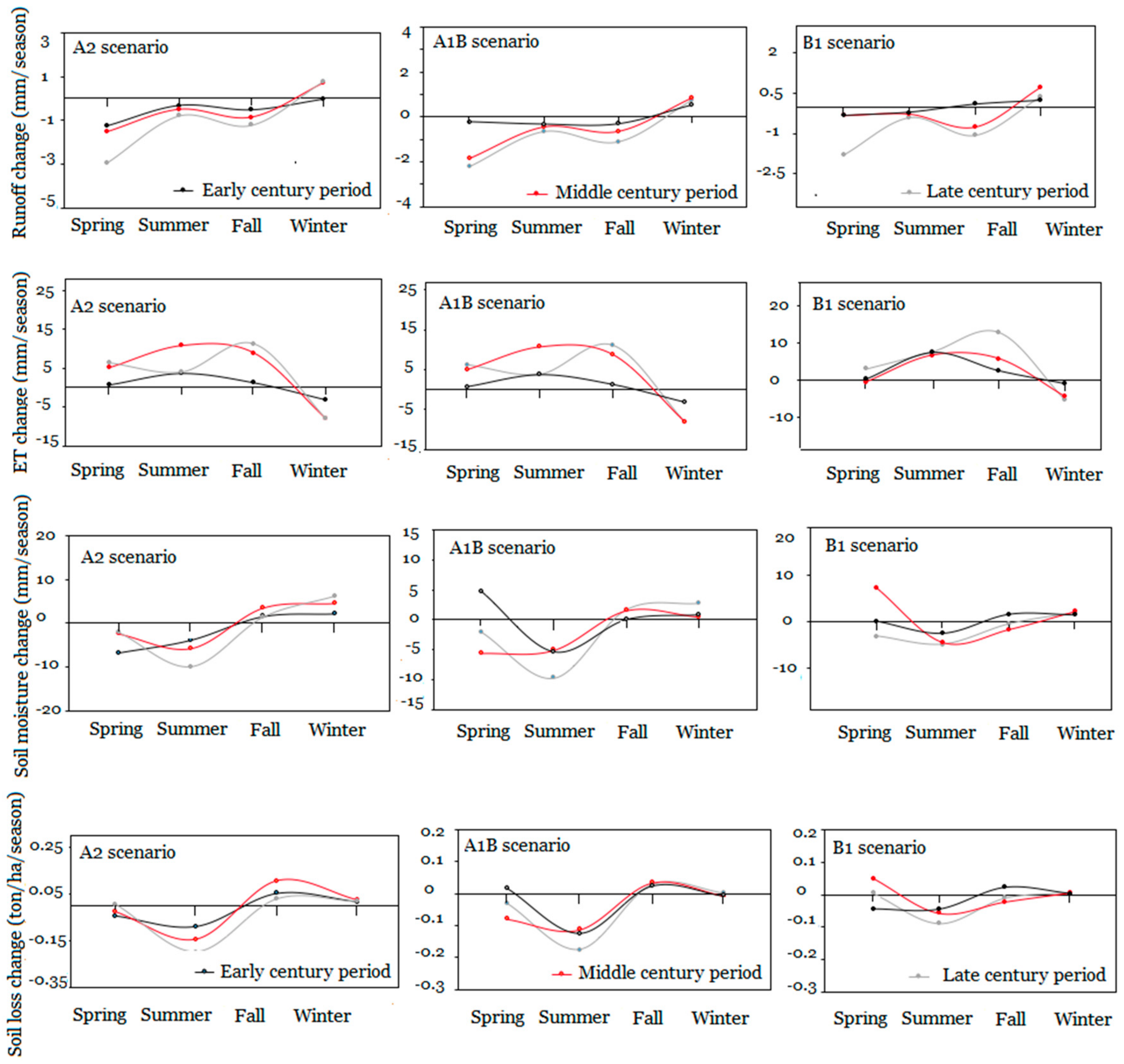
Temporally, seasonal runoff of the entire study domain has similar changing trends with precipitation, as it is projected to decrease in spring and summer, and increase in fall and winter through three future periods under the A2 and A1B scenarios, while runoff increases only in winter under the B1 scenario. Summer runoff decreases due to the precipitation reductions and air temperature increases which elevate the ET and decrease the soil moisture over three future periods (Figure 6). Spring runoff reduction is attributed to the air temperature rise as well. Winter runoff has the greatest increase over the four seasons as the result of the increased precipitation and air temperatures over three future periods. Increased winter air temperature changes precipitation from snow toe rainfall [12,45]. Snow is predicted to decrease around 31.4% to 44.7% by Bosch et al. [45] in four watersheds around Lake Erie in the early and middle century periods. Fall runoff has the second greatest increase over the four seasons, even though fall precipitation increases were greatest, as increased fall air temperatures greatly elevate ET and decrease soil moisture (Figure 6). The projected seasonal runoff increase in fall and winter is lower than the decrease in summer and spring, therefore, the annual runoff is reduced as a result of the uneven seasonal distribution of precipitation changes and air temperature rise, even though the annual precipitation increases over the three future periods.

Spatially, forestland runoff has the same changing trend with the precipitation change, as it increases annually with seasonal increases in spring, fall, and winter and decreases in summer. Runoff from croplands and grasslands decreases annually due to the greater decreases in spring and summer and lower increase in fall and winter. The runoff decline in spring and summer is caused by the combined effects of the air temperature increase and precipitation reduction, while lower runoff increases in fall and winter are caused by the precipitation increase and air temperature rise (

Table 7. Seasonal changes of runoff and soil loss over three future periods under A2 scenario.

Runoff (mm Season−1)	Cropland			Forestland			Grassland
	Early	Middle	Late	Early	Middle	Late	Early	Middle	Late
Spring	−17.53	−9.85	−13.86	−4.11	4.00	11.70	−3.85	−3.36	−6.10
Summer	−8.69	−14.72	−23.44	−4.19	−4.62	−10.85	−1.65	−2.30	−3.15
Fall	3.57	7.15	3.00	1.72	4.75	1.76	0.55	0.98	0.38
Winter	5.15	7.00	9.05	2.19	8.27	12.60	0.91	1.50	1.73
Sum	−17.51	−10.42	−25.25	−4.39	12.41	15.21	−4.04	−3.18	−7.14
Soil Loss (Ton ha−1 Season−1)	Cropland			Forestland			Grassland
	Early	Middle	Late	Early	Middle	Late	Early	Middle	Late
Spring	-0.15	−0.10	−0.03	0.01	0.02	0.07	−0.02	−0.03	−0.03
Summer	−0.30	−0.49	−0.67	−0.01	−0.02	−0.03	−0.03	−0.03	−0.04
Fall	0.18	0.36	0.10	0.01	0.02	0.01	0.01	0.02	0.01
Winter	0.06	0.08	0.05	0.002	0.01	0.01	0.003	0.01	0.01
Sum	−0.21	−0.15	−0.55	0.012	0.03	0.06	-0.037	−0.03	−0.05

). Therefore, the uneven seasonal changes of precipitation and air temperature rise are the major reasons for the runoff decreases of croplands and grasslands.

3.4. Analysis of Soil Loss under Climate Change

Annual soil loss has consistently changing trends with runoff, as it is projected to decrease over three future periods by 0.43 ton ha⁻¹ (4.98%) to 1.80 ton ha⁻¹ (21.41%) with the greatest decrease in the late century period under the three SRES scenarios (Table 5). Temporally, the seasonal soil loss of the entire study domain increases in fall and winter, while it decreases in spring and fall over the three future periods. The magnitude of seasonal soil loss increased in fall and winter is less than the reduction in summer and winter, therefore, the annual soil loss decreases under A2 scenario (Figure 6). Spatially, annual soil loss increases in the forest areas, while it decreases in the crop and grass areas through the three future periods (Table 6), particularly, in the areas around the Mississippi Valley covered with grasses and crops (Figure S1). The increased soil loss in the forest areas of lesser magnitude than the soil loss reduction in the crop and grass areas, therefore, the annual soil loss of the entire study domain decreases over the three future periods.

Temporally, projected seasonal soil losses of the entire study domain have the same changing trends with runoff and precipitation with increases in fall and winter and decreases in summer over three future periods under the A2 scenario (Table 7, Figure 6). Fall and winter have increased soil loss due to the increase of precipitation and runoff (Table 7). Soil loss has a greater increase in the fall than in winter with the lower fall runoff, due to the increase of extreme storm events in intensity and frequency in the fall [44]. Summer soil loss reductions mainly occur due to the precipitation decrease over the three future periods (Table 7). Spring soil loss decreases were mainly due to air temperature increases that decreased runoff because of greater ET and lower soil moisture levels (Figure 6). The magnitude of soil loss reductions in the summer and spring are greater than the soil loss increases in the fall and winter, therefore, the annual soil loss decreased. Both the A1B and B1 scenarios have soil loss increases in the fall and winter respectively, which were different from the two seasons of soil loss increases for A2.

Spatially, projected seasonal soil loss changes of forestlands are the same as the precipitation and runoff changes, with soil loss increases in spring, fall, and winter due to the precipitation increase, and decreases in the summer due to the precipitation decrease (Table 7). Seasonal soil loss of the grass and crop areas has similar changing trends with runoff, as it increases in the fall and winter, while it decreases in the spring and summer. Soil loss decreases in the spring and summer are mainly due to the air temperature rise and precipitation reduction respectively, and increases in fall and winter are a result of precipitation increases. Annual soil loss of forestlands increases due to the precipitation increase, while crop and grass areas have decreased soil loss as a result of precipitation decreases in summer and air temperature rise (Table 7). As the annual soil loss reduction of crop and grass areas is greater than the increased quantity of forestlands, projected annual soil loss over the three land covers decreases throughout the three future periods.

3.5. Impacts of Steep Slopes on Soil Loss Responses to Climate Change

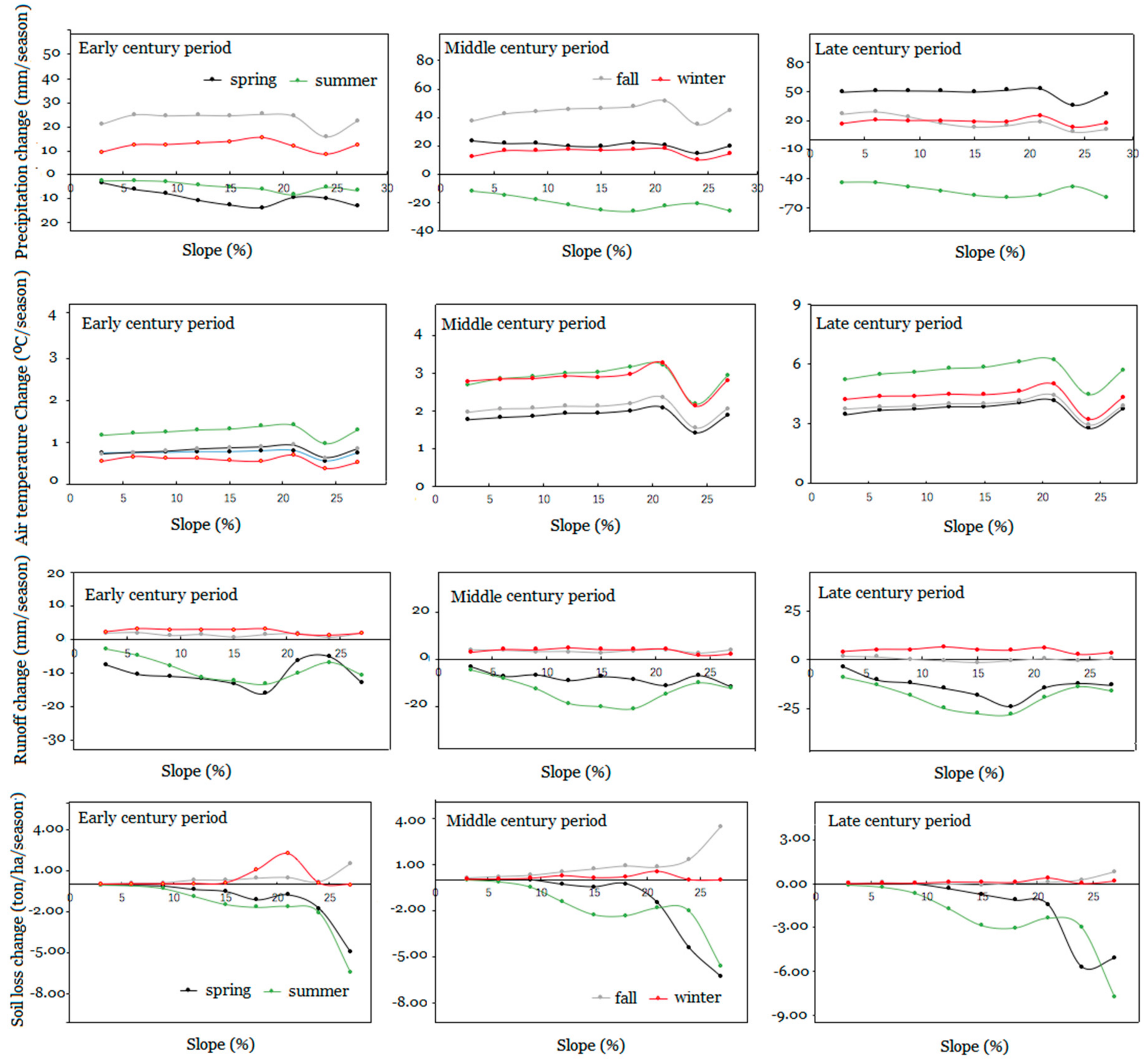
Greater projected changes in soil loss were predicted in the southern study domain where the Mississippi River Valley is located (Figure S1). Therefore, changes in precipitation, air temperatures, runoff, and soil loss are plotted with the slopes in Figure 7 under the A2 scenario. No obvious precipitation changes are indicated with slope variation, while air temperatures show greater increases over steep slopes (>10%) than flat slopes (<10%). Runoff in spring and summer decreases with the slope gradient and has greater reductions over steep slopes than flat slopes, and no obvious changes are detected for runoff in the fall and winter. The greater runoff decrease over steep slopes in spring and summer is attributed to the greater air temperature rise which decreases the soil moisture and increases the ET over steep slopes.

Soil loss has greater projected decreases on the steeper slopes than the flatter slopes in the spring and summer, particularly in the late century periods due to the greater air temperature rise. Fall and winter soil losses were greater on the steeper slopes than the flatter ones, even though they have slight increases in the late century period. Steep slopes make soil loss more sensitive to climate changes, particularly, in the spring and summer over the three future periods (Figure 7). Therefore, it makes sense that areas around the Mississippi River Valley with greater soil loss are projected to decrease in the spring and summer, but increase in the fall and winter (Figure S2).

4. Discussion

The projected annual precipitation of the Great Lakes region increases under three SRES scenarios and seasonal precipitation increases in spring, fall, and winter, while it decreases in summer over three future periods under the A2 and A1B scenarios. Air temperature increases constantly over the three future periods with the greatest increase in summer over all four seasons. Annual runoff decreases over the three future periods due to the air temperature increase together with unequal precipitation changes over the four seasons. Runoff decreases in spring and summer as a result of the precipitation reduction and air temperature rise, while it increases in the fall and winter due to the precipitation increase. This finding is close to that of Cousino et al. [46] where they projected annual flow decreases and precipitation increases in the Maumee River watershed in the Great Lakes region. Cousino et al. [46] attributed the runoff reduction to the ET increases led by the air temperature increase, as the runoff decreases for three seasons in the late century period due to the substantially greater ET increases and smaller annual precipitation increases, though no seasonal analysis was provided about precipitation and runoff.

Projected annual soil loss of the Great Lakes region has similar changing trends as runoff, as it decreases over the three future periods under the three SRES scenario. Seasonal soil loss has greater decreases in spring and summer due to the combined effects of reduced precipitation and increased air temperature and it has smaller increases in fall and winter resulting from precipitation increases. Therefore, annual soil loss decreases over the entire study domain. Our finding is similar to the conclusions of Verma et al. [47] who predicted decreased annual soil loss by 3.3% to 25.8% in the middle century period based on a precipitation decrease of 3.2% with soil loss decreases in spring, summer, and fall in the Maumee River watershed of the Great Lakes region. Cousino et al. [46] found that soil losses in the same watershed were projected to decrease over the four seasons due to significantly increased ET led by the air temperature increase even though precipitation increases slightly in the middle and late century period. O’Neal et al. [11] obtained similar findings in northern Indiana with soil loss projected to decrease by 3.0% based on a runoff decrease of 26% and precipitation increase of 6.8% with a decrease in July and an increase in October.

Spatially, annual soil loss of the Great lakes region decreases due to the smaller increase in the forest areas and greater decreases in the crop and grass areas. Forest areas have increased annual soil loss mainly due to the precipitation increase, and seasonal soil loss increases in spring, fall, and winter for the same reason over three future periods under the three SRES scenarios. Crop and grass areas have decreased annual soil loss mainly due to the air temperature rise with greater seasonal soil loss decreases in spring and summer and lower increases in the fall and winter. Therefore, soil conservation management practices should be planned to reduce the impacts of precipitation increases with attention focused on the spring, fall, and winter in the forestlands, and in the fall and winter for the grasslands and croplands. Steep slopes make soil loss more sensitive to the climate change, as areas of steeper slopes had greater soil loss reductions due to the air temperature rise. The southern study domain located in the Mississippi River Valley with steeper slopes had greater projected soil loss reductions in summer due to precipitation decreases, and smaller soil loss increases in the remainder of the year due to the combined effects of increased air temperatures and precipitation.

Uncertainties exist in this study about the exact land uses and field managements in the Great Lakes region; they were held constant in this study for the future and base periods to isolate the climate change impacts on soil losses. The tillage methods, tillage dates, crops, and cropping dates may change in the future instead of being fixed for the simulations in this study. A shift to earlier crop planting dates would leave fields protected by crop canopy cover for longer time periods that likely would act to reduce runoff and soil erosion in the spring [11]. Agricultural areas are major sources of soil losses, but it is uncertain that the land use type area percentages will not change [11]. Uncertainties coming from the VIC-WEPP model application related to the model structure, inputs, and parameters are present in the estimation of soil losses. In addition, uncertainties also come from the climate model results used to make the predictions.

5. Conclusions

Response of soil loss towards future climate change was studied in the U.S. Great Lakes region for three future periods under three climate scenarios to clarify the temporal and spatial distributions of soil loss. The VIC-WEPP model was utilized to estimate the soil loss after a parameter uncertainty analysis was performed with the GLUE method at Waseca, MN. Changes in projected precipitation, air temperature, runoff, and soil loss were analyzed at seasonal and annual time steps for the entire study domain and for three major land covers.

Annual precipitation is projected to increase constantly by 0.23% to 8.6% over three future periods with seasonal precipitation increases in the spring, fall, and winter, and decreases in the summer. Air temperature is projected to increase by 0.68 °C to 4.34 °C with the greatest increase in summer followed by fall, winter, and spring. Annual runoff is projected to decrease by 0.64% to 6.39% with seasonal runoff increases in the fall and winter and decreases in the spring and summer. Runoff from the forestland in the northern study domain is projected to increase in the spring, fall, and winter due to precipitation increases and to decrease in the summer due to decreased precipitation. Runoff from crop and grass areas in the middle and southern study domain has greater projected decreases in the spring and summer and lower projected increases in the fall and winter due to the combined effects of air temperature and precipitation increases.

Annual soil loss is projected to decrease by 4.99% to 23.2% over three future periods with seasonal soil loss increases in the fall and winter and decreases in the spring and summer. Summer soil loss decline is due to the precipitation reduction and fall soil loss increase is caused by increased precipitation. Annual soil loss from forestland increases with seasonal soil loss increases in the spring, fall, and winter, and decreases in the summer. Soil loss from the cropland and grassland areas decreases with seasonal soil loss increases in spring and summer, and decreases in fall and winter. Soil loss from steep slopes is more sensitive to climate change as steep hillslopes have greater soil loss reductions than the flat ones in the spring and summer due to the air temperature rise.

To reduce soil loss in the Great Lakes region, soil conservation efforts should focus on the fall and winter seasons in reducing the effects of increased precipitation on cropland and grassland areas. Efforts also should be exerted in forestlands in the spring to reduce the increased soil loss caused by the precipitation increases. In future studies, the land cover changes need to be considered in the soil loss predictions and soil loss conservation strategies, as soil loss will increase at a greater rate if forestland is replaced with grassland in the northern study domain, and grassland is replaced with cropland in the southern study domain in the future, based on the hydrological responses toward land cover change of Mao and Cherkauer [27].

References

- Kling, G.W.; Hayhoe, K.; Johnson, L.B.; Magnuson, J.J.; Polasky, S.; Robinson, S.K.; Shuter, B.J.; Wander, M.M.; Wuebbles, D.J.; Zak, D.R. (Eds.) Confronting Climate Change in the Great Lakes Region: Impacts on Our Communities and Ecosystems; UCS Publications: Cambridge, MA, USA, 2003. [Google Scholar]
- Hayhoe, K.; Dorn, J.V.; Croley, T.; Schlegal, N.; Wuebbles, D. Regional climate change projections for Chicago and the U.S. Great Lakes. J. Great Lakes Res. 2010, 36, 7–21. [Google Scholar] [CrossRef]
- Cruce, T.; Yurkovich, E. Adapting to Climate Change: A Planning Guide for State Castal Managers—A Great Lakes Supplement; NOAA Office of Ocean and Coastal Resource Management: Silver Spring, MD, USA, 2011. [Google Scholar]
- Chagnon, F.J.F.; Bras, R.L. Contemporary climate change in the Amazon. Geophys. Res. Lett. 2005, 32, 1–4. [Google Scholar] [CrossRef]
- Cherkauer, K.A.; Sinha, T. Hydrologic impacts of projected future climate change in the Lake Michigan region. J. Great Lakes Res. 2010, 36, 33–50. [Google Scholar] [CrossRef]
- Trapp, R.J.; Deffenbaugh, N.S.; Brooks, H.E.; Baldwin, M.E.; Robinson, E.D.; Pal, J.S. Changes in severe thunderstorm environment frequency during the 21st century caused by anthropogenically enhanced global radiative forcing. Proc. Natl. Acad. Sci. USA, 2007, 104, 19719–19723. [Google Scholar] [CrossRef] [Green Version]
- Zhang, Y.; Hernandez, M.; Anson, E.; Nearing, M.A.; Wei, H.; Stone, J.J.; Heilman, P. Modeling climate change effects on runoff and soil erosion in southeastern Arizona rangelands and implications for mitigation with conservation practices. J. Soil Water Conserv. 2012, 67, 390–405. [Google Scholar] [CrossRef] [Green Version]
- Zhang, Y.G.; Nearing, M.A.; Zhang, X.C.; Xie, Y.; Wei, H. Projected rainfall erosivity changes under climate change from multimodel and multiscenario projections in Northeast China. J. Hydrol. 2010, 384, 97–106. [Google Scholar] [CrossRef]
- Pruski, F.F.; Nearing, M.A. Climate-induced changes in erosion during the 21st century for eight U.S. locations. Water Resour. Res. 2002, 38, 1298. [Google Scholar] [CrossRef]
- Pruski, F.F.; Nearing, M.A. Runoff and soil loss responses to changes in precipitation: A computer simulation study. J. Soil Water Conserv. 2002, 57, 7–16. [Google Scholar]
- O’Neal, R.M.; Nearing, M.A.; Vining, R.C.; Southworth, J.; Pfeifer, R.A. Climate change impacts on soil erosion in Midwest United States with changes in crop management. Catena 2005, 61, 165–184. [Google Scholar] [CrossRef]
- Sinha, T.; Cherkauer, K.A. Impacts of future climate change on soil frost in the Midwestern United States. J. Geophys. Res. 2010, 115, 1–16. [Google Scholar] [CrossRef]
- Edwards, W.M.; Owens, L.B. Large storm effects on total soil erosion. J. Soil Water Conserv. 1991, 46, 75–78. [Google Scholar]
- González-Hidalgo, J.G.; Peña-Monné, J.L.; de Luis, M. A review of daily soil erosion in Western Mediterranean areas. Catena 2007, 71, 193–199. [Google Scholar] [CrossRef]
- Nearing, M.A.; Jetten, V.; Baffaut, C.; Cerdan, O.; Couturier, A.; Hernandez, M.; le Bissonnais, Y.; Nichols, M.H.; Nunes, J.P.; Renschler, C.S.; et al. Modeling response of soil erosion and runoff to changes in precipitation and cover. Catena 2005, 61, 131–154. [Google Scholar] [CrossRef]
- Flanagan, D.C.; Nearing, M.A. (Eds.). USDA—Water Erosion Prediction Project Hillslope Profile and Watershed Model Documentation; NSERL Report No. 10; USDA-ARS National Soil Erosion Research Laboratory: West Lafayette, IN, USA, 1995. [Google Scholar]
- Flanagan, D.C.; Gilley, J.E.; Franti, T.G. Water Erosion Prediction Project (WEPP): Development history, model capabilities, and future enhancements. Trans. Am. Soc. Agric. Biol. Eng. 2007, 50, 1603–1612. [Google Scholar] [CrossRef]
- Nearing, M.A.; Wei, H.; Stone, J.J.; Pierson, F.B.; Spaeth, K.E.; Weltz, M.A.; Flanagan, D.C.; Hernandez, M. A rangeland hydrology and erosion model. Trans. Am. Soc. Agric. Biol. Eng. 2011, 54, 901–908. [Google Scholar] [CrossRef]
- Zhang, X.C.; Nearing, M.A. Impact of climate change on soil erosion, runoff, and wheat productivity in central Oklahoma. Catena 2005, 61, 185–195. [Google Scholar] [CrossRef]
- Mao, D.; Cherkauer, K.A.; Flanagan, D.C. Development of a coupled soil erosion and large-scale hydrology modeling system. Water Resour. Res. 2010, 46, 1–15. [Google Scholar] [CrossRef]
- Liang, X.; Lettenmaier, D.P.; Wood, E.F.; Burges, S.J. A simple hydrologically based model of land surface water and energy fluxes for general circulation models. J. Geophys. Res. 1994, 99, 14415–14428. [Google Scholar] [CrossRef]
- Liang, X.; Lettenmaier, D.P.; Wood, E.F. One-dimensional statistical dynamic representation of subgrid variability of precipitation in the two-layer variable infiltration capacity model. J. Geophys. Res. 1996, 101, 403–422. [Google Scholar] [CrossRef]
- Cherkauer, K.A.; Bowling, L.C.; Lettenmaier, D.P. Variable infiltration capacity cold land process model updates. Glob. Planet. Chang. 2003, 38, 151–159. [Google Scholar] [CrossRef]
- Flanagan, D.C.; Frankenberger, J.R.; Ascough, J.C., II. WEPP: Model use, calibration, and validation. Trans. Am. Soc. Agric. Biol. Eng. 2012, 55, 1463–1477. [Google Scholar] [CrossRef]
- Flanagan, D.C.; Nearing, M.A. Sediment particle sorting on hillslope profiles in the WEPP model. Trans. Am. Soc. Assoc. Eng. 2000, 43, 573–583. [Google Scholar] [CrossRef]
- Miller, D.A.; White, R.A. A conterminous United States multi-layer soil characteristics data set for regional climate and hydrology modeling. Earth Interact. 1998, 2, 1–26. [Google Scholar] [CrossRef]
- Mao, D.; Cherkauer, K.A. Impacts of land-use change on hydrologic responses in the Great Lakes region. J. Hydrol. 2009, 374, 71–82. [Google Scholar] [CrossRef]
- Knutti, R.; Sedlacek, J. Robustness and uncertainties in the new CMIP5 climate model projections. Nat. Clim. Chang. 2013, 3, 369–373. [Google Scholar] [CrossRef]
- Wuebbles, D.; Meehl, G.; Hayhoe, K.; Karl, T.R.; Kunkel, K.; Santer, B.; Wehner, M.; Colle, B.; Fischer, E.M.; Fu, R.; et al. CMIP5 climate model analyses: climate extremes in the United States. In Climate Change 2013: The Physical Science Basis. Working Group 1 (WG1) Contribution to the 5th Assessment Report (AR5) of the Intergovernmental Panel on Climate Change (IPCC); Bulletin of the American Meteorological Society; Stocker, T.F., Qin, D., Plattner, G.-K., Tignor, M.M.B., Allen, S.K., Boschung, J., Nauels, A., Xia, Y., Bex, V., Midgley, P.M., Eds.; Cambridge University Press: Cambridge, UK, 2013. [Google Scholar]
- Mohammed, I.N.; Bomblies, A.; Wemple, B.C. The use of CMIP5 data to simulate climate change impacts on flow regime within the Lake Champlain Basin. J. Hydrol. Reg. Stud. 2015, 3, 160–186. [Google Scholar] [CrossRef]
- Nakicenovic, N.; Grübler, A.; Gaffin, S.; Jung, T.-T.; Kram, T.; Morita, T.; Pitcher, H.; Riahi, K.; Schlesinger, M.; Shukla, P.R.; et al. IPCC SRES revisited: a response. Energy Environ. 2003, 14, 187–214. [Google Scholar] [CrossRef]
- Stouffer, R.J.; Broccoli, A.J.; Delworth, T.L.; Dixon, K.W.; Gudgel, R.; Held, I.; Hemler, R.; Knutson, T.; Lee, H.-C.; Schwarzkopf, M.D.; et al. GFDL’s CM2 global coupled climate models. Part IV: Idealized climate response. J. Clim. 2006, 19, 723–740. [Google Scholar] [CrossRef]
- Delworth, T.L.; Broccoli, A.J.; Rosati, A.; Stouffer, R.J.; Balaji, V.; Beesley, J.A.; Cooke, W.F.; Dixon, K.W.; Dunne, J.; Dunne, K.A.; et al. GFDL’s CM2global coupled climate models. Part I: Formulation and simulation characteristics. J. Clim. 2006, 19, 643–674. [Google Scholar] [CrossRef]
- Gordon, C.; Cooper, C.; Senior, C.A.; Banks, H.; Gregory, J.M.; Johns, T.C.; Mitchell, J.F.B.; Wood, R.A. The simulation of SST, sea ice extents and ocean heat transports in a version of the Hadley Centre coupled model without flux adjustments. Clim. Dyn. 2000, 16, 147–168. [Google Scholar] [CrossRef]
- Pope, V.D.; Gallani, M.L.; Rowntree, P.R.; Stratton, R.A. The impact of new physical parameterizations in the Hadley Centre climate model: HadAM3. Clim. Dyn. 2000, 16, 123–146. [Google Scholar] [CrossRef]
- Washington, W.M.; Weatherly, J.W.; Meehl, G.A.; Semtner, A.J., Jr.; Bettge, T.W.; Craig, A.P.; Strand, W.G., Jr.; Arblaster, J.M.; Wayland, V.B.; James, R.; et al. Parallel Climate Model (PCM) control and transient simulations. Clim. Dyn. 2000, 16, 755–774. [Google Scholar] [CrossRef]
- Bhat, K.B.; Haran, M.; Terando, A.; Keller, K. Climate projections using Bayesian model averaging and space-time dependence. J. Agric. Biol. Environ. Stat. 2011, 16, 606–628. [Google Scholar] [CrossRef]
- Wood, A.W.; Leung, L.R.; Sridhar, V.; Lettenmaier, D.P. Hydrologic implications of dynamical and statistical approaches to downscaling climate model outputs. Clim. Chang. 2004, 62, 1–3. [Google Scholar] [CrossRef]
- Nicks, A.D.; Lane, L.J.; Gander, G.A. Weather generator. In USDA-Water Erosion Prediction Project: Hillslope Profile and Watershed Model Documentation; Flanagan, D.C., Nearing, M.A., Eds.; USDA-ARS National Soil Erosion Research Laboratory: West Lafayette, IN, USA, 1995. [Google Scholar]
- Kandel, D.D.; Western, A.W.; Grayson, R.B.; Turral, H.N. Process parameterization and temporal scaling in surface runoff and erosion modeling. Hydrol. Process. 2004, 18, 1423–1446. [Google Scholar] [CrossRef]
- Nash, J.E.; Sutcliffe, J.V. River flow forecasting through conceptual models: Part 1. A discussion of principles. J. Hydrol. 1970, 10, 282–290. [Google Scholar] [CrossRef]
- Willmott, C.J. On validation of models. Phys. Geogr. 1981, 2, 184–194. [Google Scholar]
- Beven, K.J.; Binley, A. The future of distributed hydrological models: model calibration and uncertainty prediction. Hydrol. Process. 1992, 6, 279–298. [Google Scholar] [CrossRef]
- Wang, L.; Cherkauer, K.A.; Flanagan, D.C. The role of cold season process on soil erosion in Great Lakes Region. In Proceedings of the American Society of Agronomy, Crop Science Society of America and Soil Science Society of America (ASA-CSSA-SSSA) International Annual Meeting, Cincinnati, OH, USA, 23 October 2012. [Google Scholar]
- Bosch, N.S.; Evans, M.A.; Scavia, D.; Allan, J.D. Interacting effects of climate change and agricultural BMPs on nutrient runoff. J. Great Lakes Res. 2014, 40, 581–589. [Google Scholar] [CrossRef]
- Cousino, L.K.; Becker, R.H.; Zmijewski, K.A. Modeling the effects of climate change on water, sediment, and nutrient yields from the Maumee River watershed. J. Hydrol. Reg. Stud. 2015, 4, 762–775. [Google Scholar] [CrossRef]
- Verma, S.; Bhattarai, R.; Bosch, N.S.; Markus, M. Climate change impacts on flow, sediments and nutrient export in a Great Lakes watershed using SWAT. Clean Soil Air Water 2015, 11, 1464–1474. [Google Scholar] [CrossRef]
Figure 1.
Great Lakes region states.
Figure 2.
Modern land cover map of three states within the Great Lakes region together with watersheds and gauge stations for model hydrological calibration [21].
Figure 3.
DEM of the Great Lakes region.
Figure 4.
Uncertainty analysis of VIC-WEPP model in simulating soil loss at Waseca, MN.
Figure 5.
Seasonal changes of precipitation and air temperature over four seasons throughout three future periods under three SRES scenarios.
Figure 6.
Seasonal changes of soil moisture, ET, runoff, and soil loss changes over three future periods under three SRES scenarios.
Figure 7.
Seasonal changes of precipitation, air temperature, runoff, and soil loss with slope gradients in cropland under the A2 scenario.