Improvement of Hydroclimatic Projections over Southeast Spain by Applying a Novel RCM Ensemble Approach


1
Department of Civil Engineering, R&D Group of Water Resources Management, Universidad Politécnica de Cartagena, Paseo Alfonso XIII, 52, 30203 Cartagena, Spain
2
Departmento de Ingeniería Civil, Grupo de Investigación Ciencia e Ingeniería del Agua y el Ambiente, Facultad de Ingeniería, Pontificia Universidad Javeriana, Carrera 7 No. 40-62, 110231 Bogotá, Colombia
*
Author to whom correspondence should be addressed.
Water 2018, 10(1), 52; https://doi.org/10.3390/w10010052
Submission received: 28 November 2017
/
Revised: 27 December 2017
/
Accepted: 7 January 2018
/
Published: 10 January 2018
(This article belongs to the Special Issue Sustainable Water Management within Inland River Watershed)
Abstract
:Climate model outputs can be used as climate forcing for hydrological models to study the impact of climate change on the water cycle. This usually propagates cumulative uncertainties, transferring the errors from the climate models to the hydrological models. Then, methodologies are needed to evaluate the impact of climate change at basin scale by reducing the uncertainties involved in the modeling chain. The paper aims to assess the impact of climate change on the runoff, considering a novel approach to build a Regional Climate Model (RCM) ensemble as climate forcing for a parsimonious spatially distributed hydrological model. A semiarid basin of southeast of Spain was selected for the study. The RCM ensembles were built based on seasonal and annual variability of rainfall and temperature. If the runoff projections for 2021–2050 are compared to the 1961–1990 observed period, a significant decrease in runoff equal to −20% (p-value t-test 0.05) was projected. However, by changing the observed period to 1971–2000, a despicable change (2.5%) is identified. This fact demonstrates that trends based on short records are very sensitive to the beginning and end dates, due to the natural variability. Special attention should be paid to the selection of the period for impact studies.

1. Introduction
Numerous studies identified the Mediterranean region as one of the most vulnerable areas to climatic and anthropogenic changes and to water crisis [1,2,3,4]. During the latter half of the 20th century, cumulative discharge from many mid-latitude rivers decreased by 60%, while high-latitude rivers experienced increased discharge [5]. The impacts of climate change can be exacerbated when occurring in regions with imbalances between water demands and available water resources [1], such as the southeast of Spain. Moreover, climate change has a larger effect than human activities on decreases in runoff [6], so it must be studied carefully.
For understanding the plausible impacts of climate change on hydrological processes and water availability, the regional climate models (RCMs) and the global climate models (GCMs) are valuable tools, simulating precipitation, temperature and wind speed, among other variables. Nevertheless, the uncertainties in the climate projections, such as unknown future greenhouse gas emissions [7] and the simplified representation of processes, are still high [8,9].
Usually, two approaches are used to characterize the uncertainties of climate projections: perturbed physics ensembles [10] and multi-model ensembles generated with different initial and boundary conditions [11,12]. On the one hand, some authors calculate multi-model ensembles as a simple mean of several models [13]. On the other hand, the use of weighted averages where the model weight depends on some measure of performance, and several techniques to assess the performance of each model, are widely applied [14,15,16,17,18,19,20,21,22]. Considering this last approach, the performance of two novel approaches to build RCM ensembles of monthly precipitation over Spain was evaluated [23]. While [23] found the best ensemble approximation was based on the modified Reliability Ensemble average method [16,21] for weighting the ensemble RCM members.
Another problem with climate model output is the systematic error or bias between historical observations and climate model hindcast [24]. Bias correction methods are increasingly applied in climate model studies and serve to overcome this error [24,25]. The mean bias of the statistics of daily precipitation simulated by five RCMs was evaluated by [24]. While [25] applied a bias correction of projected precipitation, provided by three RCMs and potential evapotranspiration projections, as input to a simple hydrological model. However, when many climate models are considered and the interdependency is important, other solutions should be taken into account. The building of RCM ensembles based on the performance to reproduce a historical period implicitly penalizes (less weight in the ponderation) those RCMs which exhibit higher bias in relation to the historical dataset. Therefore, it should be considered as an indirect method to take into account the bias or systematic errors, with the advantages of spatial assessment.
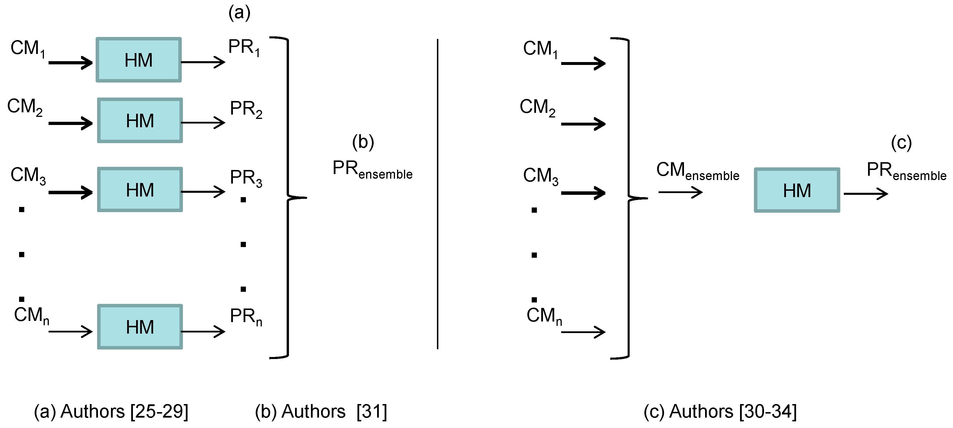
Due to both problems of uncertainty of climate projections, there are different strategies in reducing uncertainties (Figure 1). On the one hand, many researchers [25,26,27,28,29] investigate the impact of climate change on future water resources employing a hydrological model (HM) driven by one specific climate model (CM), as it is presented in Figure 1a. Then, a hydrological projection ensemble (PRensemble) could be built from the results of each simulation (Figure 1b). However, the effects of variability of precipitation and temperature from all available CMs have not been evaluated.
On the other hand, the assessment of climate change impacts on water resources using RCM and GCM ensembles and hydrological models has become an important challenge around the world [30,31,32,33,34] (Figure 1c). A multi-model average ensemble approach from 11 GCMs was used by [30] to drive a macroscale hydrology model in the Colorado River Basin. While [32] assessed actual evapotranspiration and streamflow with the Soil and Water Assessment Tool (SWAT) model in a subtropical Chinese basin for the 21st century. These authors used multi-model average ensemble approach from six GCMs (where each member is assigned by an equal probability of occurrence). An increase of the annual mean actual evapotranspiration ensemble and decrease of the annual mean streamflow compared to the baseline period (1971–1999) were projected [32]. In these works, although attempts to reduce climatic uncertainties have been made using average climate ensembles, the main weaknesses are related to the large hydrological uncertainties due to the parameterization of complex hydrological models. For example, both SWAT model used by [32,34], and Variable Infiltration Capacity (VIC) used by [30,33], present a large number of parameters and some of them are difficult to obtain.
However, there is no systematic approach available for reducing the combined uncertainty in streamflow projections from both climate projections and hydrological models [31]. These authors proposed three different approaches, and concluded that reducing climate input uncertainty (combining climate models, Figure 1c) provides better results than multi-model streamflow forecasts (Figure 1b). Since the multi-model streamflow is obtained by combining the results from a single hydrological model driven by individual climate projections (Figure 1b).
In the present work, robust RCM ensembles of rainfall, minimum and maximum temperature were built based on the revisited REA method proposed by [24], giving different weights to RCMs according to their performance in simulating the yearly and seasonal present climate. In other words, the time series of the selected meteorological variables were built on seasonal and yearly timescales, then empirical Cumulative Density Functions (CDFs) were fitted. The reliability factors for each RCM were computed as the p-value of the two sample Smirnov–Kolmogorov tests (TSSK) between the RCM data and the observed dataset. Finally, the greater TSSK p-value defines the higher weight of the RCM in the final ensemble, because the final performance criterion is a combination of the reliability factors.
Then, with the aim to reduce the uncertainties in the hydroclimatic projections, a hydrological distributed model with only four parameters was forced by the climate ensemble (monthly precipitation and temperature) over the semiarid Segura River Basin (southeast of Spain). This basin presents the greater water scarcity of Spain, and it is usually affected by severe droughts.
In addition, the sensitivity of hydrometeorological projections to historical period selection has been evaluated. Two time periods have been considered for the analysis, the common 1961–1990 and 1971–2000. The latter one was affected by a strong El Niño event according to [35], and it was employed by several authors [32]. The authors [36] found good predictability when El Niño–Southern Oscillation (ENSO) indexes were used to forecast dry events in the Mediterranean coast of Spain. Several authors summarize the influence of some climatic indexes over the Iberian Peninsula, and pointed out that the positive phase of North Atlantic Oscillation (NAO) index is related with below normal rainfall amounts over the Iberian Peninsula [37]. Also, [37] indicated that the warming trends of climate would lead in more positive phases of NAO, which likely explain the precipitation negative trends over the Iberian Peninsula.
To the best of our knowledge, there are no published works considering distributed hydrological models driven by RCM ensembles based on seasonal and annual variability of meteorological variables, in semiarid water-stressed basins with strong problems relating to water scarcity and droughts. This type of approach constitutes a way to reduce the uncertainties involved in the climate and hydrological models, giving more support to the decision-making process. This is especially important in semiarid basins, such as the Segura River Basin and its headwaters basin, which have a high vulnerability to water stress and a fragile balance between water resources and demands. A particular case study was selected among the several headwaters of Segura River Basin: the Fuensanta Basin, which is one of the most important sources of water resources for the Murcia region in Spain.
The present work is organized into five sections. The description of the used dataset and a deeper description of the study area are presented in Section 2. Section 3 discusses the methodological aspects of the climate model ensemble building, hydrological model and calibration and validation procedures. The main results of the research are presented in Section 4, and finally the conclusions are presented in Section 5.
2. Study Area and Datasets
2.1. Study Area
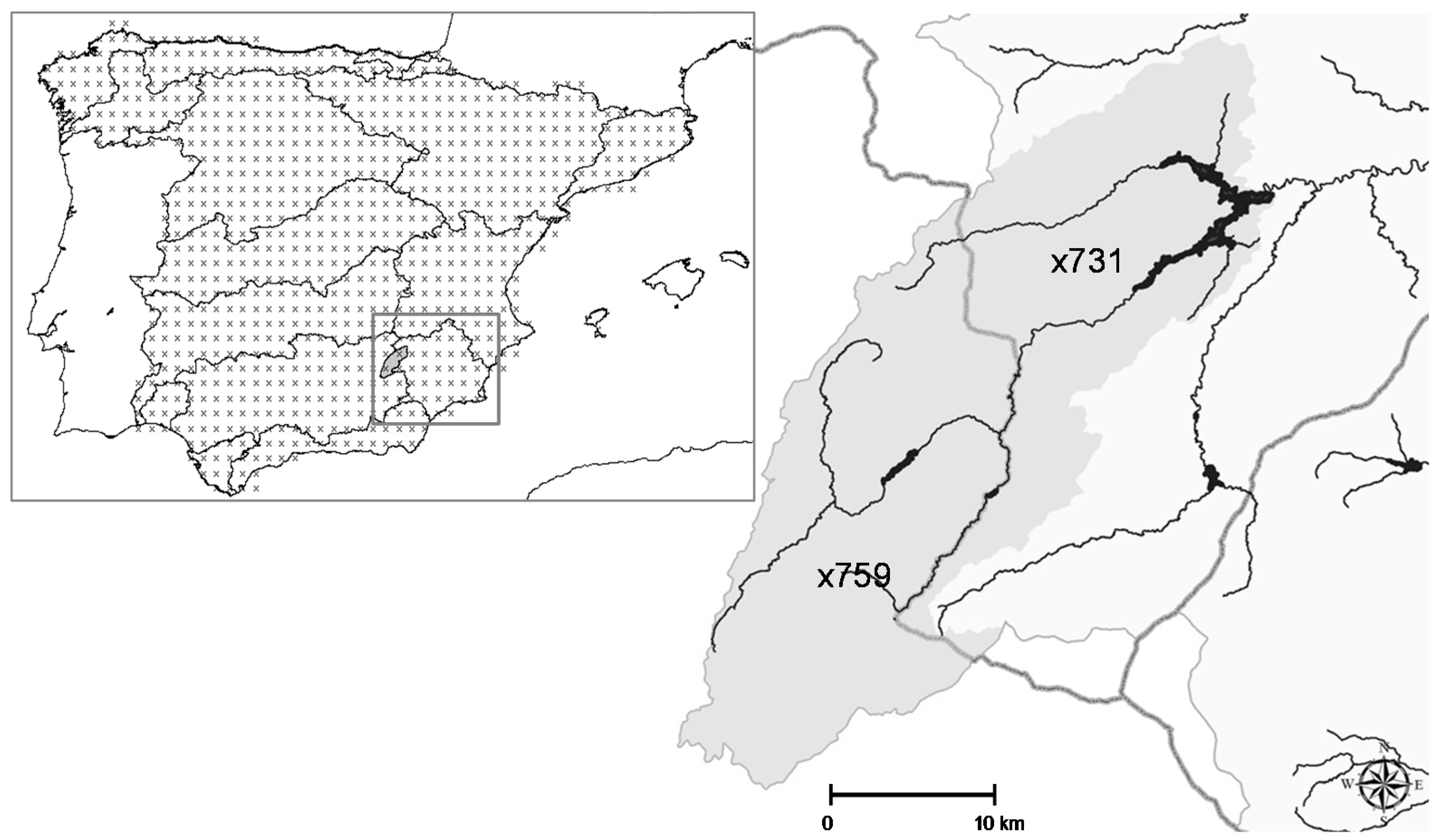
The variability of rainfall in the southeast of Spain can reach extreme irregularity. Rains are more frequent in autumn (between October and December). The study region corresponds to the Segura River Basin (SRB), with a surface area of 18,900 km2; it is located in the semiarid southeast corner of the Iberian Peninsula (Figure 2). Average precipitation in the region ranges from 1000 mm/year in the headwater areas to 300 mm/year in the driest lowlands, while the potential average evapotranspiration is approximately 1400 mm/year. The main characteristic of the SRB is its water scarcity, considering the available water resources and the high agricultural and urban demands. The water exploitation index with a value of 237.2% [1], estimated from the mean annual runoff and mean annual total water demand, is the highest of all Spanish basins. The available water resource per inhabitant is only 442 m3/inhabitant/year for SRB, therefore the gap between water supply and demand is extremely high. In consequence, this basin is considered as one of the most water-stressed regions in the western Mediterranean basin. Consequently, the water transfers from other basins together with desalinization are considered the most attractive options to increase water availability in the basin. Moreover, recurrent and frequent drought periods (1980–1982, 1993–1995, and 2005–2008) have generated important crises and greatly complicated water management.
Once the RCM ensembles were obtained for temperature and rainfall projections over SRB, the impact analyses on hydrological projections were focused on the contribution of the basin to the Fuensanta River Reservoir (named Fuensanta Basin). Fuensanta Basin, located in the headwater of the Segura River Basin (Figure 2), covers an area of 1220.6 km2 with an average altitude of 1263 m. This basin is one of the main sources of water for the whole Segura River Basin. Therefore, the strategic location of the Fuensanta Basin makes it one of the most suitable for studies of impacts on runoff generation, and thus for improving the understanding of the climate change impacts in all economic activities and livelihoods of the region.
2.2. Datasets
The high-resolution observational dataset of temperature and rainfall (1961–2007), named Spain02, was provided by [38]. The regular grid presents 0.2° of spatial resolution. This dataset was extended in the Segura River Basin, for the period 2008–2013, considering the meteorological stations provided by several institutions such as SIAM (Sistema de Información Agraria de Murcia) [39], SIAR (Servicio Integral de Asesoramiento al Regante de Castilla La Mancha) [40], and IVIA (Instituto Valenciano de Investigaciones Agrarias) [41].
Sixteen RCMs from ENSEMBLES European project [42], driven by different GCMs for scenario A1B [7], were used (Table 1). This dataset presents 0.25° of spatial resolution for the 1961–2050 period. Considering the climate effects of SRES (Special Reports on Emission Scenarios) and RCP (Representative Concentration Pathways) scenarios, [43] indicate that the median of the projected warming to the end of the century under the SRES A1B scenario is found between RCP6 and RCP8.5 scenarios. Analyzing mean temperature and precipitation change, [44] found a very high spatial correlation between RCP8.5 and A1B results, with 0.82–0.97 for temperature changes and 0.59–0.92 for precipitation changes depending on the region for mid-century, and even stronger correlation for both parameters towards the end of the century.
The data of observed runoff for calibration in the Fuensanta Basin was provided by the Segura River Basin authority (CHS, Hydrographic Confederation of Segura River Basin).
3. Method
3.1. Building PDF Ensemble
The ensemble probability density function (PDF) was built following the next steps. Firstly, the monthly time series of precipitation and temperature were obtained for each grid point from the RCMs and observed data. Secondly, the reliability factor (R) was calculated using a measure to compare the agreement among the cumulative density functions (CDFs) of each RCM and from observed data on 1961–1990. Thirdly, R was used to obtain the normalized reliability factor (Pm). Finally, the ensemble PDF was estimated using the normalized reliability factor Pm as the weighting factor.
The revisited REA method [23] was proposed to build the RCM ensembles of temperature and precipitation. The REA method has been applied in several studies [16,45,46,47]. This method is a flexible tool to assess the mean, uncertainty range, and the production of probabilistic outcomes of the ensemble climate change from both GCMs and RCMs.
The original REA method [15,16] calculates reliability weights (Ri) for different models as a product of two reliability factors: model performance criterion (RB), which represents the capability of each model to represent observed climate; and convergence criterion (RD), which evaluate the distance of a projected change to the ensemble average. Therefore, the reliability factor for model i is calculated as follows [15]:
where the parameters m and n are the criterion weights.
Due to the difficulty for assessing the convergence criterion, because the reference probability density functions (PDFs) for future climate are not known, several authors [21,23,48] eliminated RD from the definition of reliability factor.
In the present work, the estimation of the reliability factor Ri is addressed by a novel approach based on seasonal and yearly cumulative density probabilities (CDFs), proposed by [23] as follows:
where 1 ≤ i ≤ number of RCMs.
Equation (2) states that each model weight is given by the multiplication of five functional factors (RWinter, RSpring, RSummer, RAutumn and RYearly) to measure the model ability as a function of the model bias for reproducing the seasonal (winter, spring, summer and autumn) and annual mean variability of present climate. Furthermore, the bias analysis is based in the assessment of p-value from the well-known two sample Smirnov–Kolmogorov test [49], between RCM CDFs and observed data CDFs for the historical period (1961–1990). Therefore, the p-value is considered as a metric to compute the reliability factors Rwinter, Rspring, Rsummer, Rautumn and Ryearly. Previous works successfully considered this metric to build RCM ensembles for the analysis of dry spell lengths [25,45].
The CDFs from the observational datasets represent the reference in this period. The inverse of the Weibull equation was used to compute the empirical quantiles of CDF.
The values of Ri were estimated in the grid points defined over Segura River Basin with a 0.25° of spatial resolution (Figure 2), and were interpolated applying the Kriging method for each model. The spatial distribution of the normalized reliability factor (Pmi) was obtained for each RCM from the maps of Ri, as follows [16]:
where j = 1 to N, and N is the number of RCMs.
The Pmi is the likelihood of each RCM. Then, based on Pmi as a weighting factor, the PDF ensembles (or CDF ensembles) was built on site 2021–2050 horizons, giving greater weight to RCMs with a high value of the Pm. The spatial interpolations methods named inverse distance weighting (IDW) and ordinary kriging presented a similar performance in the case of scarce spatial autocorrelation of the studied variable for complex terrain areas [50], because both are distance-based methods. The weights for the IDW are usually proportional to the inverse of the squared distance between the prediction point and the observation points. The precision of this geometric method is affected by the number of the closest neighboring samples. While kriging calculates the values of weights by estimating the spatial structure of the variable’s distribution represented by a sample semivariogram. In the present case, the spatial representation of the studied variable obtained by the geostatistical method (kriging) was more realistic, therefore it was the selected method for the spatial interpolations. The assumption about the spatial correlation of the data implies that the closer the points are, the more similar are their values. Another relevant strength of kriging method is the ability to take into account the directional bias of data, which was expected because of the complex topography of studied region. Finally, the kriging method is a statistical method which computes the most likely value to interpolate, according to the spatial correlation which is considered trough the semivariogram. On the other hand, the IDW method does not take into account that spatial structure of data.
3.2. Hydrological Model and Its Calibration and Validation
A continuous, conceptual, and distributed hydrological model with few parameters, named the Témez model developed by [51], is applied. This model, which is widely applied in Spain [52], simulates monthly average flows in natural regime at any point of the drainage network.
The total runoff is produced from the rainfall not retained in the soil’s upper layer, and not evaporated. The monthly model reproduces the essential water transport processes that occur in the different phases of the hydrological cycle, and establishes the principle of continuity and sharing laws and water transfers between different storages.
The meteorological input to the model corresponds to the datasets of precipitation (P) and potential evapotranspiration (PET). Information about sub-basins and maps of hydrogeological units are also required for model parameterization (Hmax: maximum soil holding capacity; Imax: maximum infiltration rate; C: runoff coefficient; and α: aquifer discharge coefficient). As output, the model generates the spatial distributions of runoff, infiltration, soil water, and actual evapotranspiration.
In this study, before calibration, three parameters (Hmax, Imax and α) were specified considering recommendations from [53]. The parameter C was defined according to [54] guidelines.
Observed hydrometeorological datasets were considered to calibrate and validate the Témez model in the Fuensanta Basin. For calibrating the model, a representative period of six years (2000–2005) was used, where land cover was provided by CORINE Land Cover 2006 [55]. During the time period 2000–2005, dry and wet years were observed with maximum and minimum flow rate fluctuations. In consequence, the parameters obtained in calibration phase are considered more robust and better able to represent both wet and dry years.
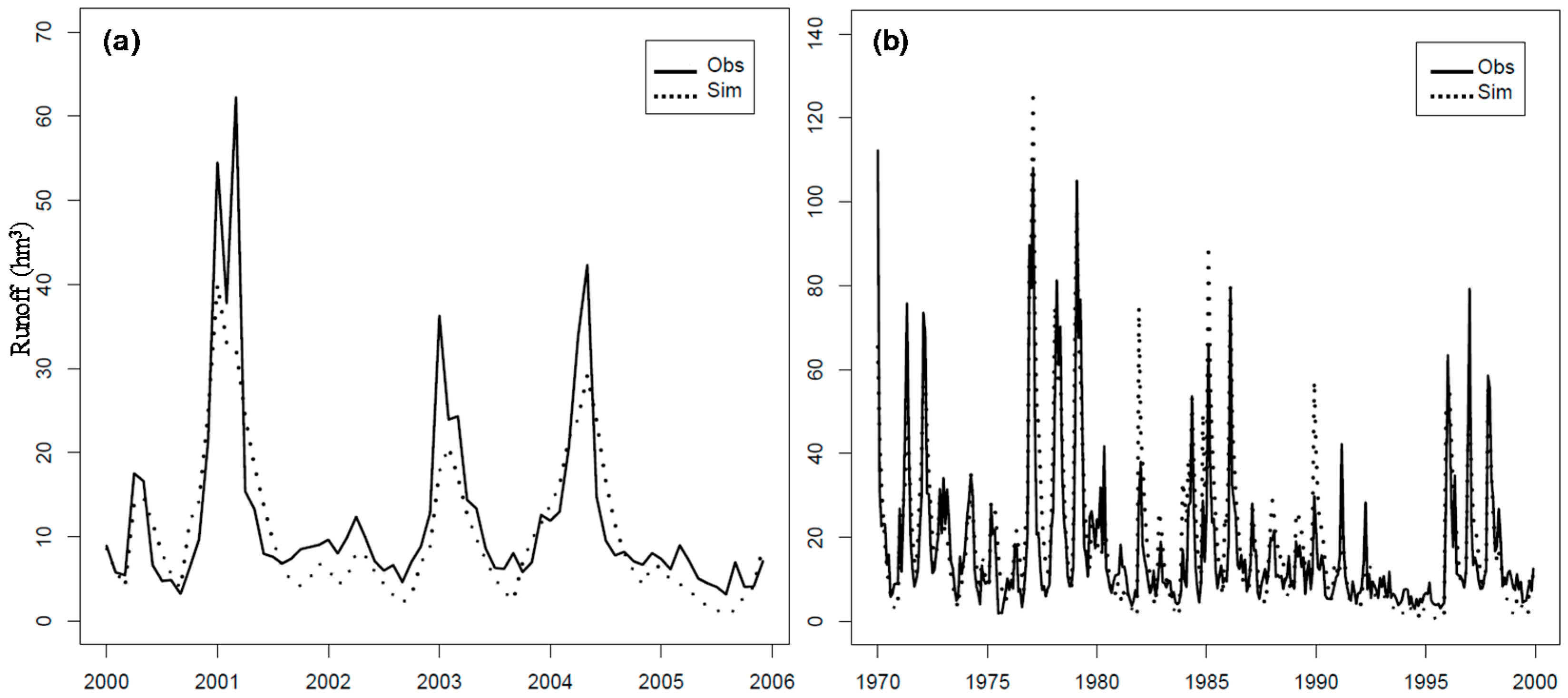
Calibration parameters were defined by minimizing the differences between observed runoff provided by the Segura River Basin authority (CHS) and simulated runoff by the model. The performance analysis was based on graphical and numerical goodness-of-fit, considering the Nash–Sutcliffe efficiency value (NSE) [56]. The comparison between the observed and simulated hydrograph for the calibration phase in the period 2000–2005, at Fuensanta Reservoir Station (Figure 3a), demonstrates a good fit with a NSE value of 0.71. Then, the validation of the hydrological model was performed for a period of 30 years, from 1970 to 1999 (Figure 3b), with satisfactory results (NSE equal to 0.732). A limitation of hydrological models is the degree of predictability, that is, there is no assurance that a model obtains good performance when it is used under conditions different from those of the calibration period [57]. In the present work, the selected calibration period was 5 years. Nevertheless, the validation process for a long period of 30 years demonstrates the good predictability of the model by the performance and reliability achieved [58].
Assessment of Potential Evapotranspiration
Different PET input estimated by several methods (Penman–Monteith, Hargreaves–Samani, Jensen–Haise, and Hamon methods), can produce similar runoff simulations in both dry and humid regions [59]. Therefore, the temperature-based Hargreaves–Samani model [60] can be considered as an alternative to the Penman–Monteith model [61] when only air temperature records are available to calculate PET. However, several studies [62,63] have shown that the Hargreaves–Samani model overestimates reference evapotranspiration (ET0) values in humid regions and underestimates them in dry regions. For this reason, other studies have even proposed new parametric expressions to calculate the adjusted Hargreaves coefficient [64,65,66].
The spatial distribution of ET0 is estimated from the observational dataset of temperature Spain02 and from the RCM ensembles of temperature, applying the method explained previously (Equation (2)), considering the Hargreaves model adjusted to the study area [64]:
where ET0 is the reference evapotranspiration (mm day−1); Ra is the water equivalent of the monthly-averaged daily extraterrestrial radiation (mm day−1), obtained from tables based on the latitude and month according to [61] where 1 mm day−1 = 0.408 × MJulio/m2/day; Tmax and Tmin are the monthly-averaged maximum and minimum values of daily air temperature (°C); and Tm is the monthly-averaged daily temperature, calculated as the average of Tmax and Tmin.
4. Results
4.1. RCM Ensembles
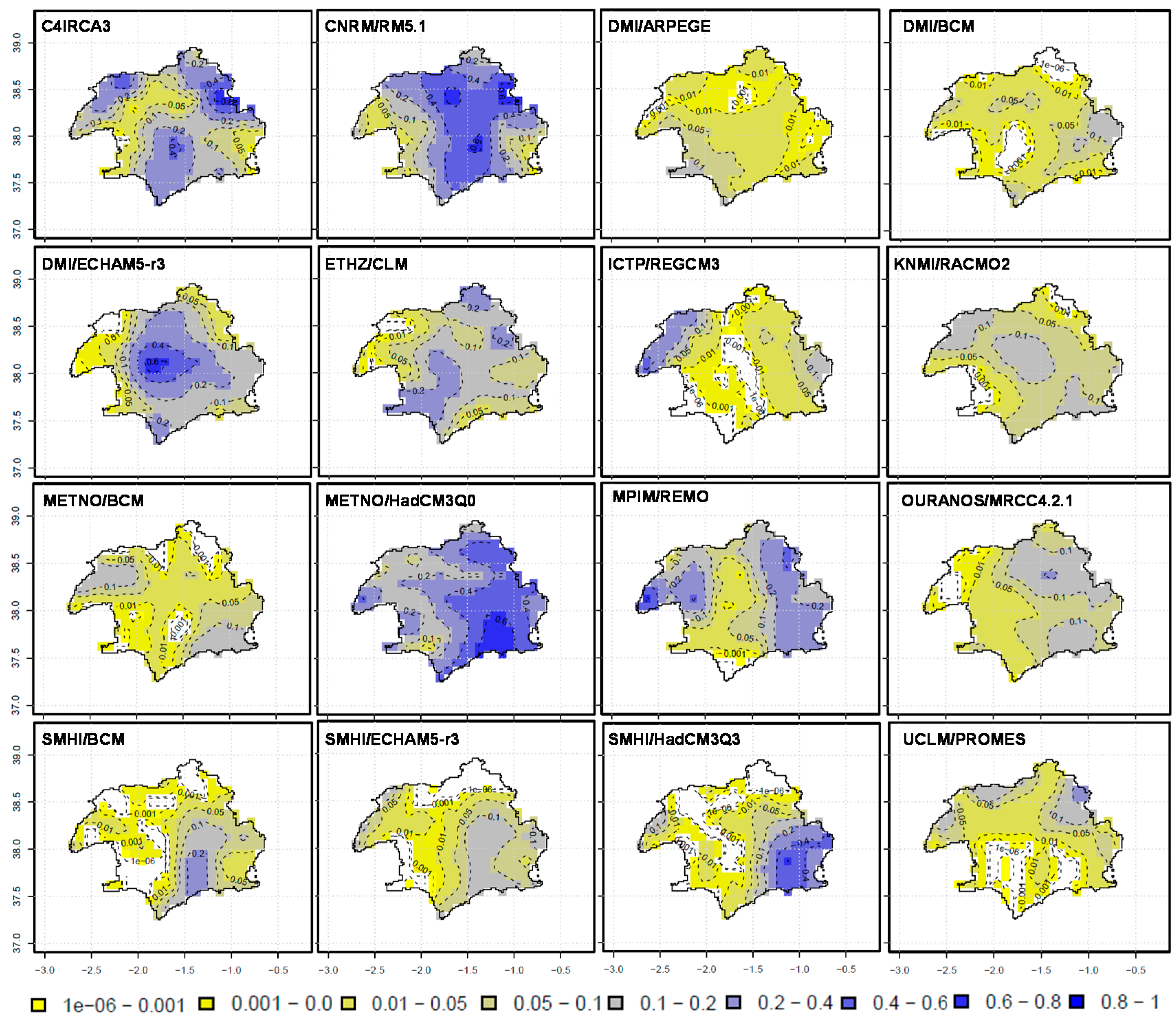
The kriging interpolation method was applied to obtain the maps of reliability factor (Ri). Figure 4 presents the results in Segura River Basin for Ri for each of the RCMs in the case of the rainfall variable. The strengths and weaknesses of each RCM could be identified from the spatial distributions of values of Ri, presented in Figure 4 and estimated with the Equation (2). Therefore, the RCMs with satisfactory skills (in blue) to simulate the observed data in the Segura River Basin are the following: C4IRCA3, CNRM/RM5.1, DMI/ECHAM5-r3, ETHZ/CLM and METNO/HadCM3Q0. The models with worse performance according to the obtained results (lower values of Ri in Figure 4, in yellow), are DMI/ARPEGE, DMI/BCM, SMHI/BCM, SMHI/ECHAM5-r3, SMHI/HadCM3Q3 and UCLM/PROMES.
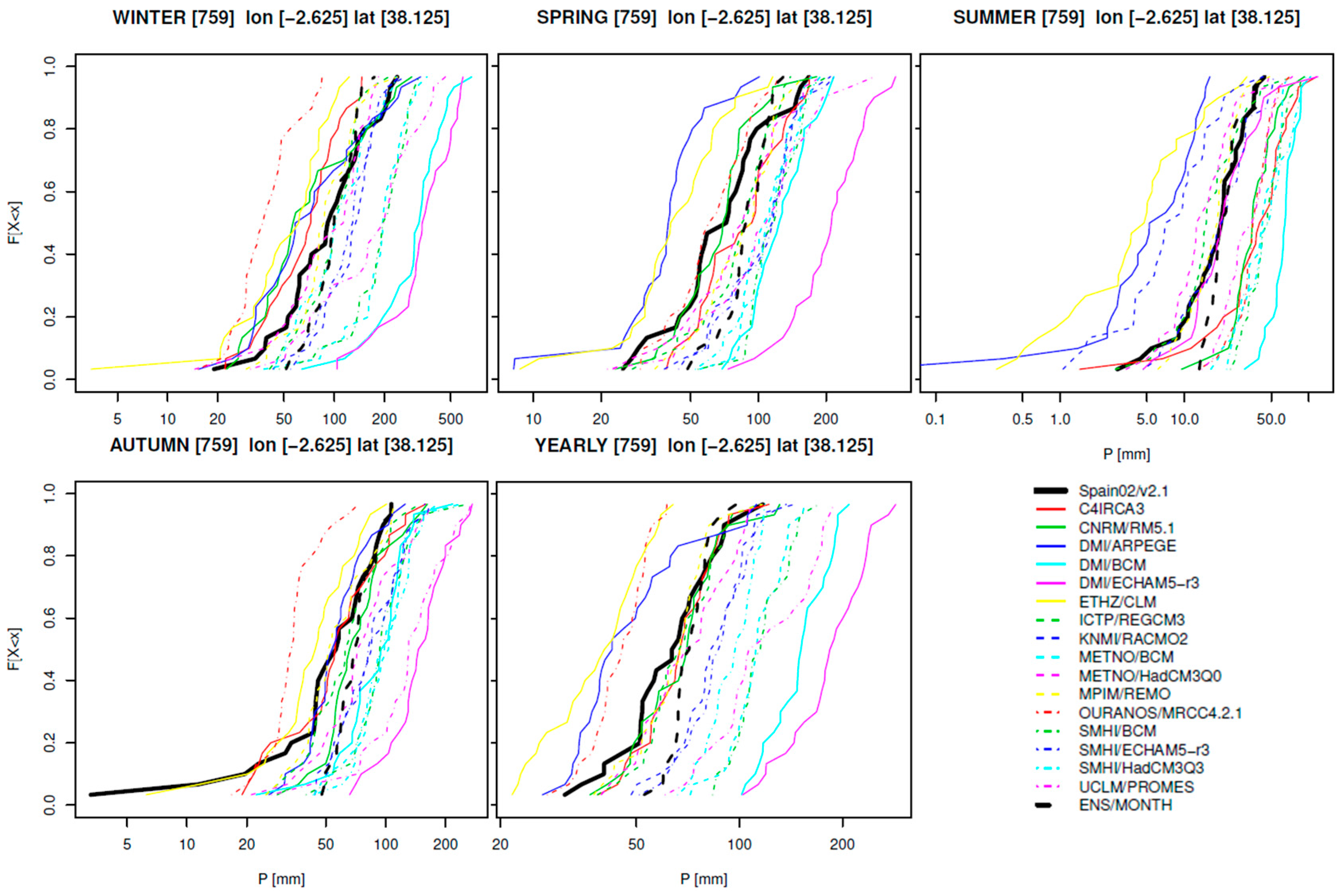
The CDFs of rainfall, minimum and maximum temperature for each RCM, and observational datasets, were obtained. Then, the CDF ensemble was built on each site of the study region, applying the methodology described in Section 3.1. Figure 5 presents a detail of results for seasonal and yearly rainfall on site 759 (Fuensanta Basin). The CDF ensemble in general captures well the seasonal and annual variability of observed rainfall, with more adjusted results in winter and summer (Figure 5).
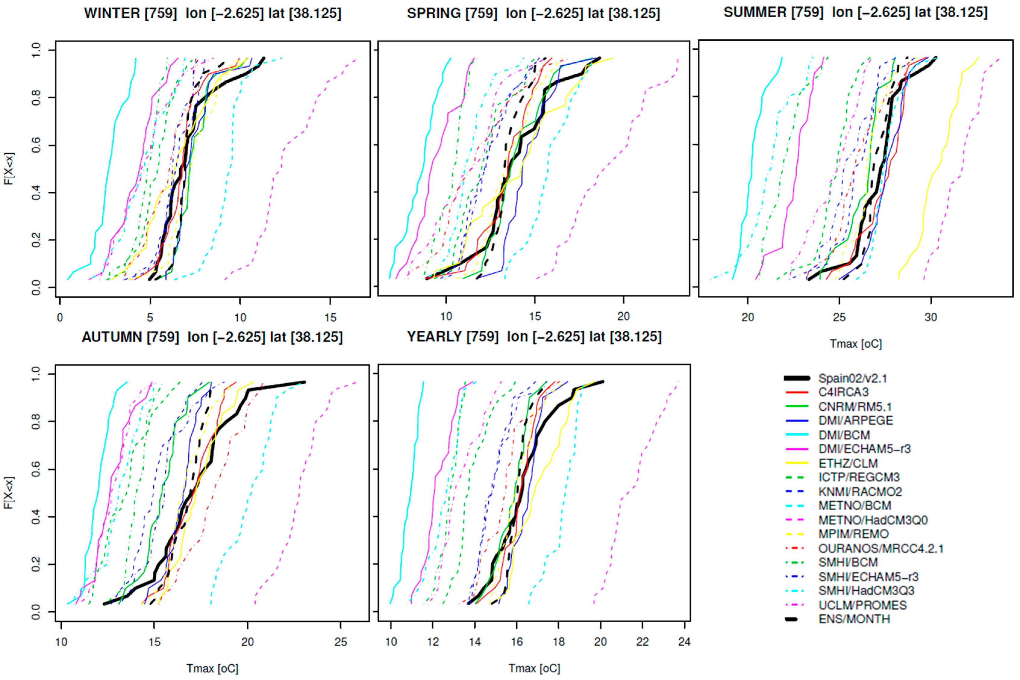
In the case of maximum temperature CDFs on the same site (Figure 6), the goodness-of-fit between the CDF ensemble and Spain02 CDF is satisfactory. The best results correspond to the summer season and at yearly scale (0.794 and 0.522 p-values respectively). While for winter, spring and autumn the p-values are not satisfactory (0.134 winter, 0.366 spring, and 0.135 autumn).
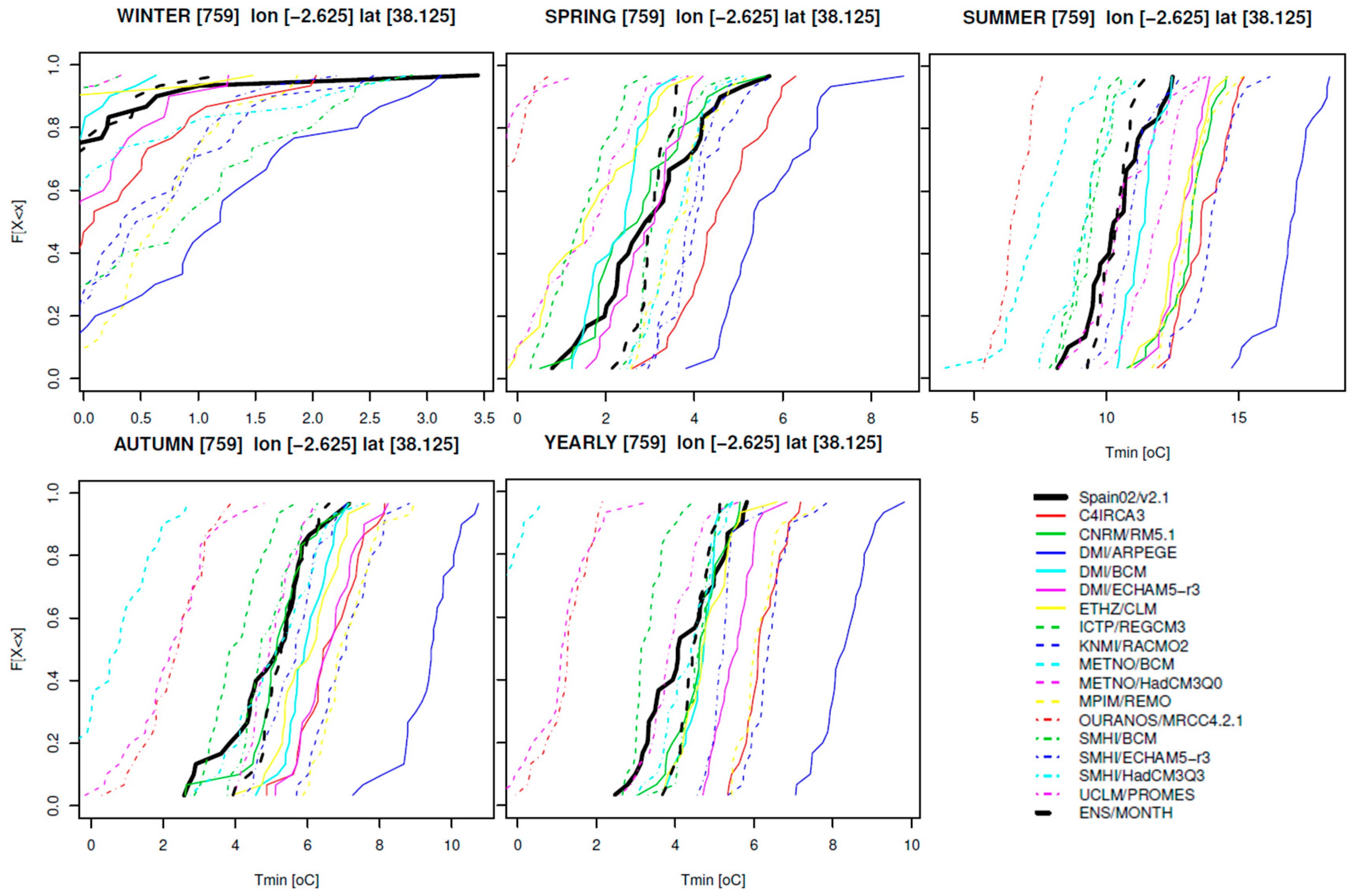
For minimum temperature, the greatest differences between the Spain02 CDF and CDF ensemble occur in winter and at yearly scale (0.06 and 0.04 p-values), and the lowest differences in the summer season (0.634 p-value) (Figure 7). It is noteworthy (Figure 5, Figure 6 and Figure 7) that the best performance varies for each analyzed season, site, and variable, and that there are instances where a single model performs better than the ensemble. However, this fact is not generalizable, and the ensemble approach in general reduces the bias compared to the single model approach.
A more exhaustive analysis of the sites and p-values for rainfall over Spain is presented in [23].
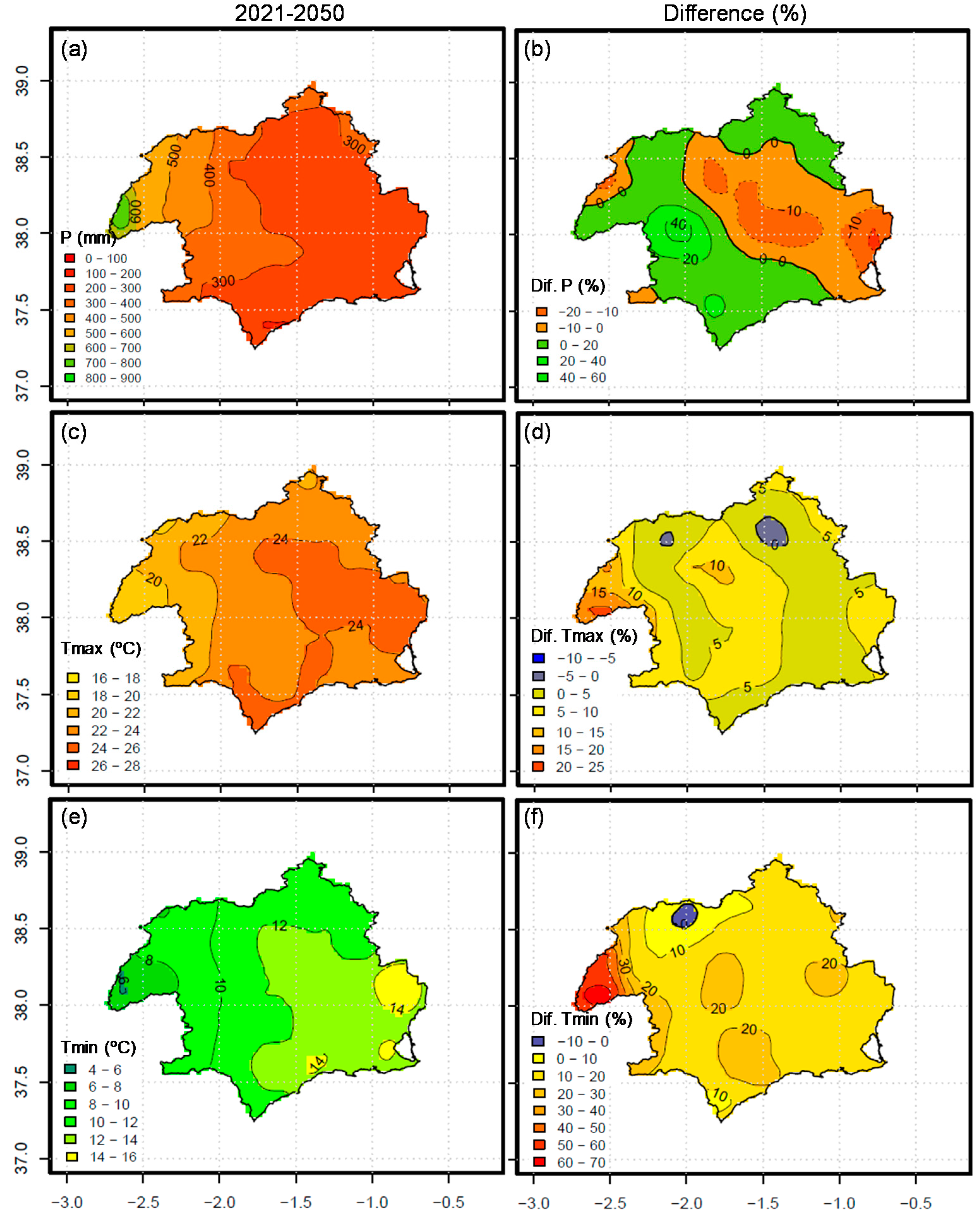
The maps of RCM ensemble projections for mean annual rainfall (P), maximum temperature (Tmax), and minimum temperature (Tmin) for 2021–2050 period, and the differences (%) with respect to the 1961–1990 period, are presented in Figure 8. A decreasing gradient of P from west-east is expected for 2021–2050 (Figure 8a), with the highest P values corresponding to the Fuensanta Basin (above 800 mm/year) and minimum values in the coast (less than 300 mm/year). The Tmax and Tmin (Figure 8c,e) have a spatial distribution with a strong increasing west-east gradient. Focusing on the difference maps (Figure 8b), decreases of P for 2021–2050 are expected in the middle east and some parts of the northwest, while increases (greater than 20%) in the southwest and north areas. On the other hand, the Tmax (Figure 8d) is predicted to increase by 10% to 20% in the Fuensanta Basin, while an increase of 5% on average is expected for the rest of the basin. Finally, a general increase in the Tmin (Figure 8f), of between 10% and 20% is expected for most of the Segura River Basin, while in the Fuensanta Basin the highest increases are identified (greater than 60%).
4.2. Trends for Meteorological and Hydrological Variables for 2021–2050 Horizon
Once calibrated and validated for the Fuensanta basin, the Témez hydrological model was used to obtain the hydrological projections driven by the RCM ensembles (rainfall and potential evapotranspiration) previously generated applying the methodology described in Section 3.1. The runoff projections were obtained for the period 1961–2050.
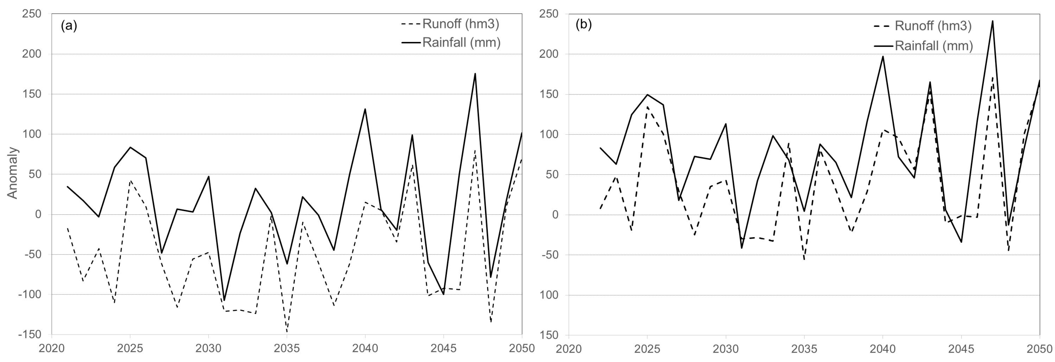
Figure 9 presents the projected anomalies of rainfall and runoff for the time period 2021–2050, related to the mean of the periods 1961–1990 and 1971–2000. The difference between the means from both time periods was estimated. The t-test was used to determine if the two means were significantly different from each other. In Table 2, the p-value of t-test is presented in parenthesis, identifying the significant differences (denoted by * in Table 2). If the mean annual runoff for the future (2021–2050) is compared with the historical dataset for 1961–1990 (Figure 9a), a plausible significant decrease (−20%) is expected (Table 2). However, from Figure 9a, the decrease of runoff is more clearly identified in the first part of the period. If the comparison is based on the difference between 2021–2050 and 1971–2000 period (Figure 9b), the expected trend of runoff would be positive (2.5% from Table 2). Analyzing the other variables in the hydrological cycle, the reduction of runoff for 2021–2050 (Table 2) in relation with the baseline period (1961–1990) is justified in the reduction of rainfall and the increase of PET (≈4%). However, for 2021–2050 in relation to 1971–2000, an increase in rainfall over 11% and a similar increase of PET (≈3.7%) are expected.
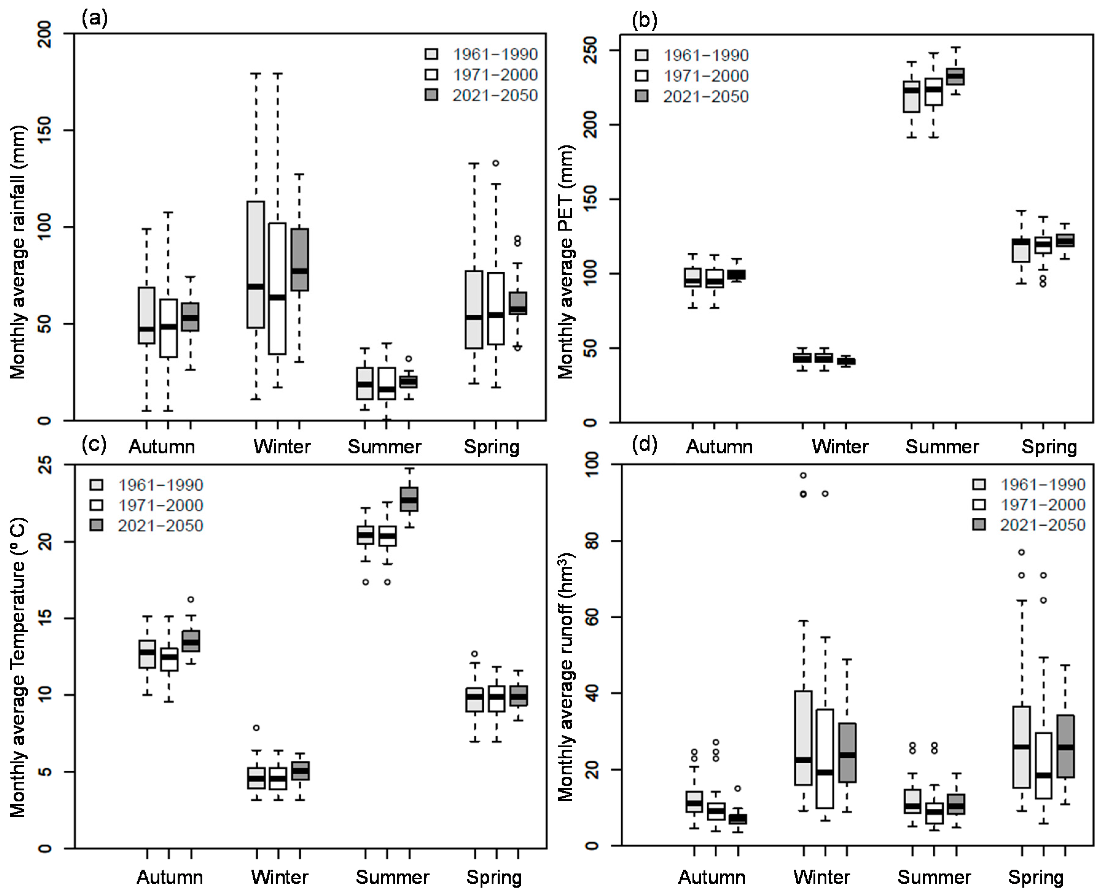
The variability of the simulated seasonal mean rainfall, PET, mean temperature and runoff for the Fuensanta Basin, in two observed (1961–1990 and 1971–2000) and one future (2021–2050) time periods, were comparatively analyzed (Figure 10). If the results for 2021–2050 are contrasted with the corresponding results for the observational periods 1961–1990 and 1971–2000, a lower range of variability of the mean of rainfall, PET, and temperature for the future, are expected. Nevertheless, in the case of future runoff, this trend is not detected. In Figure 10a, increases in the median rainfall (although not in the maximum value) are expected for all seasons in the period 2021–2050, in contrast with 1961–1990. However, these increases are greater in the case of contrast with the observed period 1971–2000. In the case of PET (Figure 10b), clear increases in the minimum, maximum, first, third quartile, and median are only expected in summer in 2021–2050 with respect to both observational periods. These results match the summer boxplot of the mean temperature (Figure 10c). In Figure 10d, contrasting the future period with the observational periods, a significant decrease in the runoff in autumn is identified. However, if the future scenario of runoff is contrasted with the 1971–2000 period, a clear increase in the median in winter, spring and summer is predicted.
Figure 11 presents the spatial distributions of predicted changes in annual rainfall, potential evapotranspiration and runoff for 2021–2050 period, in relation to 1961–1990 and 1971–2000 historical periods. In the case of contrast with the period 1961–1990 (Figure 11a), important decreases of rainfall are identified because this historical period was wetter. Consequently, the decreases in runoff (Figure 11e) are higher and cover a wider area, in comparison with the contrast results from the time period 1971–2000 (Figure 11f). In this last case, the runoff decreases are only identified in the lower part of the basin.
The maps of PET projections relative to 1961–1990 (Figure 11c) and 1971–2000 (Figure 11d) historical periods are spatially consistent. A general increase of PET (4% on average) in the majority of the basin and a decrease in some small areas from 0 to 5% are expected.
In summary, increases in mean temperature and PET are expected for the 2021–2050 period in contrast to the 1961–1990 historical dataset, especially in summer and autumn. Variations in precipitation are expected according to observed period and season. Finally, reductions in runoff, especially in autumn, are expected in the future with respect to both observed periods. However, with respect to the 1971–2000 period, increases in runoff for winter, summer and spring are projected.
5. Discussion and Conclusions
In this study, the average runoff decreases significantly for the 2021–2050 period in comparison with 1961–1990. The mean annual runoff reduction (20%) is mainly explained by the significant increase of mean annual evapotranspiration (4%), rather than the reduction of mean annual precipitation. However, if the 1971–2000 period is selected for comparison, a divergent trend (positive trend) is detected, although without significant differences. This fact demonstrates the high sensitivity of the results to the time period selected for comparison, where specific events could influence the results and conclusions. As an example, for 1971–2000, although two periods of severe drought (1980–1982 and 1993–1995) were observed, a strong El Niño occurred at the end of the period 1971–2000.
Therefore, in concordance with [37], trends based on short records are very sensitive to the beginning and end dates and do not in general reflect long-term climate trends. Moreover, due to the natural variability, special attention should be paid to the selection of the period for analysis of the impacts
It should be highlighted that the negative impacts of climate change on water cycle will be exacerbated in semi-arid basins with water shortages, which will have important implications for water management. By building RCM ensembles of meteorological data that are used as climate forcing for a parsimonious hydrological model, the reliability of hydrological projections in a semi-arid basin is increased.
Summarizing, from the results the following conclusions can be drawn:
- A new methodology for reducing the uncertainties involved in the modeling chain, from the RCMs to hydrological models, is presented.
- The seasonal and annual variability of climate variables considered in the RCM ensembles are well captured by the proposed novel approach.
- Taking into account the built RCM ensembles of rainfall and PET, different trends in runoff are detected depending on the comparison period.
- Therefore, the hydroclimatic trends are very sensitive to small changes in the climate drivers and the selection of the baseline period.
Acknowledgments
This work is one of the results of the research project 19527/PI/14 funded by Seneca Foundation-Agency of Science and Technology of Murcia Region in the framework of PCTIRM 2011–2014. The authors also acknowledge to Secretary of Research of the Spanish Ministry of Economy and Competitiveness (MINECO) and FEDER funds under Grant CGL2012-39895-C02-01 HYDROCLIM; and to Spanish Ministry of Education, Culture and Sport for Mobility Grant of Senior Professors and Researchers under Grant PRX14/00748.
Author Contributions
The authors applied and developed algorithms, and wrote the paper. The authors contributed in similar dedication to this work.
Conflicts of Interest
The authors declare no conflict of interest.
References
- Estrela, T.; Pérez-Martin, M.A.; Vargas, E. Impacts of climate change on water resources in Spain. Hydrol. Sci. J. 2012, 57, 1154–1167. [Google Scholar] [CrossRef]
- Ramos, M.C.; Balasch, J.C.; Martínez-Casasnovas, J.A. Seasonal temperature and precipitation variability during the last 60 years in a Mediterranean climate area of Northeastern Spain: A multivariate analysis. Theor. Appl. Climatol. 2012, 110, 35–53. [Google Scholar] [CrossRef]
- Milano, M.; Ruelland, D.; Dezetter, A.; Fabre, J.; Ardoin-Bardin, S.; Servat, E. Modeling the current and future capacity of water resources to meet water demands in the Ebro basin. J. Hydrol. 2013, 500, 114–126. [Google Scholar] [CrossRef]
- Hagemann, S.; Chen, C.; Clark, D.B.; Folwell, S.; Gosling, S.N.; Haddeland, I.; Hanasaki, N.; Heinke, J.; Ludwig, F.; Voss, F.; et al. Climate change impact on available water resources obtained using multiple global climate and hydrology models. Earth Syst. Dyn. 2013, 4, 129–144. [Google Scholar] [CrossRef]
- Milliman, J.D.; Farnsworth, K.L.; Jones, P.D.; Xu, K.H.; Smith, L.C. Climatic and anthropogenic factors affecting river discharge to the global ocean, 1951–2000. Glob. Planet. Chang. 2008, 62, 187–194. [Google Scholar] [CrossRef]
- Wu, J.; Miao, C.; Zhang, X.; Yang, T.; Duan, Q. Detecting the quantitative hydrological response to changes in climate and human activities. Sci. Total Environ. 2017, 586, 328–337. [Google Scholar] [CrossRef] [PubMed]
- Intergovernmental Panel on Climate Change Special Report on Emissions Scenarios. Special Report on Emissions Scenarios: A Special Report of Working Group III of the Intergovernmental Panel on Climate Change; Nakićenović, N., Swart, R., Eds.; Cambridge University Press: Cambridge, UK, 2000. [Google Scholar]
- Giorgi, F. Uncertainties in climate change projections, from the global to the regional scale. EPJ Web Conf. 2010, 9, 115–129. [Google Scholar] [CrossRef]
- Xu, C.H.; Xu, Y. The projection of temperature and precipitation over China under RCP scenarios using a CMIP5 multi-model ensemble. Atmos. Ocean. Sci. Lett. 2012, 5, 527–533. [Google Scholar]
- Murphy, J.M.; Booth, B.B.B.; Collins, M.; Harris, G.R.; Sexton, D.M.H.; Webb, M.J. A methodology for probabilistic predictions of regional climate change from perturbed physics ensembles. Phil. Trans. R. Soc. A 2007, 365, 1993–2028. [Google Scholar] [CrossRef] [PubMed]
- Tebaldi, C.; Knutti, R. The use of the multi-model ensemble in probabilistic climate projections. Phil. Trans. R. Soc. A 2007, 365, 2053–2075. [Google Scholar] [CrossRef] [PubMed]
- Diallo, I.; Sylla, M.B.; Giorgi, F.; Gaye, A.T.; Camara, M. Multimodel GCM-RCM Ensemble-Based Projections of Temperature and Precipitation over West Africa for the Early 21st Century. Int. J. Geophys. 2012, 2012, 1–19. [Google Scholar] [CrossRef]
- Murphy, J.M.; Sexton, D.M.H.; Barnett, D.N.; Jones, G.S.; Webb, M.J.; Collins, M.; Stainforth, D.A. Quantification of modelling uncertainties in a large ensemble of climate change simulations. Nature 2004, 430, 768–772. [Google Scholar] [CrossRef] [PubMed]
- Wigley, T.M.L.; Raper, C.B. Interpretation of high projections for global-mean warming. Science 2001, 293, 451–454. [Google Scholar] [CrossRef] [PubMed]
- Giorgi, F.; Mearns, L.O. Calculation of average, uncertainty range, and reliability of regional climate changes from AOGCM simulations via the ‘‘reliability ensemble averaging’’ (REA) method. J. Clim. 2002, 15, 1141–1158. [Google Scholar] [CrossRef]
- Giorgi, F.; Mearns, L.O. Probability of regional climate change based on reliability ensemble averaging (REA) method. Geophys. Res. Lett. 2003, 30, 311–314. [Google Scholar] [CrossRef]
- Dettinger, M. From climate-change spaghetti to climate-change distributions for 21st century California. San Franc. Estuary Watershed Sci. 2005, 3, 4. [Google Scholar]
- Tebaldi, C.; Smith, R.L.; Nychka, D.; Mearns, L.O. Quantifying uncertainty in projections of regional climate change: A Bayesian approach to the analysis of multimodel ensembles. J. Clim. 2005, 18, 1524–1540. [Google Scholar] [CrossRef]
- Sánchez, E.; Romera, R.; Gaertner, M.A.; Gallardo, C.; Castro, M. A weighting proposal for an ensemble of regional climate models over Europe driven by 1961–2000 ERA40 based on monthly precipitation probability density functions. Atmos. Sci. Lett. 2009, 10, 241–248. [Google Scholar] [CrossRef]
- Duan, Q.; Phillips, T.J. Bayesian estimation of local signal and noise in multimodel simulations of climate change. J. Geophys. Res. 2010, 115, D18123. [Google Scholar] [CrossRef]
- Xu, Y.; Gao, X.; Giorgi, F. Upgrades to the reliability ensemble averaging method for producing probabilistic climate-change projections. Clim. Res. 2010, 41, 61–81. [Google Scholar] [CrossRef]
- Yang, T.; Tao, Y.; Li, J.; Zhu, Q.; Su, L.; He, X.; Zhang, X. Multi-criterion model ensemble of CMIP5 surface air temperature over China. Theor. Appl. Climatol. 2017, 6, 1–16. [Google Scholar] [CrossRef]
- Olmos Giménez, P.; García Galiano, S.G.; Giraldo-Osorio, J.D. Identifying a robust method to build RCMs ensemble as climate forcing for hydrological impact models. Atmos. Res. 2016, 174, 31–40. [Google Scholar] [CrossRef]
- Frei, C.; Christensen, J.H.; Déqué, M.; Jacob, D.; Jones, R.G.; Vidale, P.L. Daily precipitation statistics in regional climate models: Evaluation and intercomparison for the European Alps. J. Geophys. Res. 2003, 108. [Google Scholar] [CrossRef]
- Karambiri, H.; García Galiano, S.G.; Giraldo, J.D.; Yacouba, H.; Ibrahim, B.; Barbier, B.; Polcher, J. Assessing the impact of climate variability and climate change on runoff in West Africa: The case of Senegal and Nakambe River basins. Atmos. Sci. Lett. 2011, 12, 109–115. [Google Scholar] [CrossRef] [Green Version]
- Thodsen, H. The influence of climate change on stream flow in Danish rivers. J. Hydrol. 2007, 333, 226–238. [Google Scholar] [CrossRef]
- Vezzoli, R.; Del Longo, M.; Mercogliano, P.; Montesarchio, M.; Pecora, S.; Tonelli, F.; Zollo, A.L. Hydrological simulations driven by RCM climate scenarios at basin scale in the Po River, Italy. In Proceedings of the International Association of Hydrological Sciences, Bologna, Italy, 4–6 June 2014. [Google Scholar] [CrossRef]
- Mbaye, M.L.; Hagemann, S.; Haensler, A.; Stacke, T.; Gaye, A.T.; Afouda, A. Assessment of Climate Change Impact on Water Resources in the Upper Senegal Basin (West Africa). Am. J. Clim. Chang. 2015, 4, 77–93. [Google Scholar] [CrossRef]
- Chattopadhyay, S.; Jha, M.K. Hydrological response due to projected climate variability in Haw River watershed, North Carolina, USA. Hydrol. Sci. J. 2016, 61, 495–506. [Google Scholar] [CrossRef]
- Christensen, N.S.; Lettenmaier, D.P. A multimodel ensemble approach to assessment of climate change impacts on the hydrology and water resources of the Colorado River Basin. Hydrol. Earth Syst. Sci. 2007, 11, 1417–1434. [Google Scholar] [CrossRef]
- Singh, H.; Sankarasubramanian, A. Systematic uncertainty reduction strategies for developing streamflow forecasts utilizing multiple climate models and hydrologic models. Water Resour. Res. 2014, 50, 1288–1307. [Google Scholar] [CrossRef]
- Sun, S.L.; Chen, H.S.; Ju, W.M.; Hua, W.; Yu, M.; Yin, Y. Assessing the future hydrological cycle in the Xinjiang Basin, China, using a multi-model ensemble and SWAT model. Int. J. Climatol. 2014, 34, 2972–2987. [Google Scholar] [CrossRef]
- Najafi, M.R.; Moradkhani, H. Multi-model ensemble analysis of runoff extremes for climate change impact assessments. J. Hydrol. 2015, 525, 352–361. [Google Scholar] [CrossRef]
- Chattopadhyay, S.; Edwards, D.R.; Yu, Y.; Hamidisepehr, A. An Assessment of Climate Change Impacts on Future Water Availability and Droughts in the Kentucky River Basin. Environ. Process. 2017, 4, 477–507. [Google Scholar] [CrossRef]
- Intergovernmental Panel on Climate Change (IPCC). Climate Change 2013: The Physical Science Basis. Contribution of Working Group I to the Fifth Assessment Report of the Intergovernmental Panel on Climate Change; Stocker, T.F., Qin, D., Plattner, G.-K., Tignor, M., Allen, S.K., Boschung, J., Nauels, A., Xia, Y., Bex, V., Midgley, P.M., Eds.; Cambridge University Press: Cambridge, UK, 2013. [Google Scholar]
- Frías, M.D.; Herrera, S.; Cofiño, A.S.; Gutiérrez, J.M. Assessing the Skill of Precipitation and Temperature Seasonal Forecasts in Spain: Windows of Opportunity Related to ENSO Events. J. Clim. 2010, 23, 209–220. [Google Scholar] [CrossRef] [Green Version]
- Rodríguez-Fonseca, B.; Rodríguez-Puebla, C. Teleconexiones climáticas en el entorno de la Península Ibérica. Predictabilidad y cambios esperados. In Clima en España: Pasado, Presente y Future; Pérez, F.F., Boscolo, R., Eds.; Ministerio de Ciencia e Innovación: Madrid, España, 2010; pp. 53–68. Available online: http://digital.csic.es/handle/10261/23600 (accessed on 5 January 2018).
- Herrera, S.; Gutiérrez, J.M.; Ancell, R.; Pons, M.R.; Frías, M.D.; Fernández, J. Development and analysis of a 50-year high-resolution daily gridded precipitation dataset over Spain (Spain02). Int. J. Climatol. 2012, 32, 74–85. [Google Scholar] [CrossRef] [Green Version]
- SIAM (Sistema de Información Agrario de Murcia). IMIDA, Región de Murcia. Available online: http://siam.imida.es/apex/f?p=101:1:689155068600146 (accessed on 20 September 2014).
- SIAR (Servicio Integral de Asesoramiento al regante de Castilla la Mancha). Available online: http://crea.uclm.es/siar/datmeteo/ (accessed on 20 September 2014).
- IVIA (Instituto Valenciano de Investigaciones Agrarias). Available online: http://www.ivia.gva.es/ (accessed on 23 September 2014).
- Christensen, J.H.; Rummukainen, M.; Lenderink, G. Formulation of Very High-Resolution Regional Climate Model Ensembles for Europe. ENSEMBLES: Climate Change and Its Impacts at Seasonal, Decadal and Centennial Timescales: Summary of Research and Results from the ENSEMBLES Project; Van der Linden, P., Mitchell, J.F.B., Eds.; Met Office Hadley Centre: London, UK, 2009; pp. 47–58.
- Zittis, G.; Hadjinicolaou, P.; Fnais, M.; Lelieveld, J. Projected changes in heat wave characteristics in the eastern Mediterranean and the Middle East. Reg. Environ. Chang. 2016, 16, 1863–1876. [Google Scholar] [CrossRef]
- Jacob, D.; Petersen, J.; Eggert, B.; Alias, A.; Christensen, O.B.; Bouwer, L.M.; Braun, A.; Colette, A.; Déqué, M.; Georgievski, G.; et al. EURO-CORDEX: New high-resolution climate change projections for European impact research. Reg. Environ. Chang. 2014, 14, 563–578. [Google Scholar] [CrossRef]
- Giraldo Osorio, J.D.; García Galiano, S.G. Assessing uncertainties in the building of ensemble RCMs over Spain based on dry spell lengths probability density functions. Clim. Dyn. 2013, 40, 1271–1290. [Google Scholar] [CrossRef]
- Torres, R.R.; Marengo, J.A. Uncertainty assessments of climate change projections over South America. Theor. Appl. Climatol. 2013, 112, 253–272. [Google Scholar] [CrossRef]
- Sun, Q.; Miao, C.; Duan, Q. Projected changes in temperature and precipitation in ten river basins over China in 21st century. Int. J. Climatol. 2015, 35, 1125–1141. [Google Scholar] [CrossRef]
- García Galiano, S.; Olmos Giménez, P.; Martínez Pérez, J.A.; Giraldo Osorio, J.D. Improving evaluation of climate change impacts on the water cycle by remote sensing ET-retrieval. In Proceedings of the International Association of Hydrological Sciences, Guangzhou, China, 24–27 August 2014; Volume 368, pp. 239–244. [Google Scholar] [CrossRef]
- Gibbons, J.D.; Chakraborti, S. Nonparametric Statistical Inference, 4th ed.; Marcel Dekker: New York, NY, USA, 2003; ISBN 9780824740528. [Google Scholar]
- Yao, X.; Fu, B.; Lü, Y.; Sun, F.; Wang, S.; Liu, M. Comparison of Four Spatial Interpolation Methods for Estimating Soil Moisture in a Complex Terrain Catchment. PLoS ONE 2013, 8, e54660. [Google Scholar] [CrossRef] [PubMed]
- Témez, J.R. Modelo Matemático de Trasformación “Precipitación-Escorrentía”; Asociación de Investigación Industrial Eléctrica (ASINEL): Madrid, España, 1977. [Google Scholar]
- CEDEX (Centro de Estudios y Experimentación de Obras Públicas). Estudio de los Impactos del Cambio Climático en los Recursos Hídricos y las Masas de Agua; CEDEX (Centro de Estudios y Experimentación de Obras Públicas), Ministerio de Agricultura, Alimentación y Medio Ambiente, Centro de Estudios Hidrográficos: Madrid, España, 2012.
- Estrela, T.; Cabezas, F.; Estrada, F. La evaluación de los recursos hídricos en el Libro Blanco del Agua en España. Ingeniería del Agua 1999, 6, 125–138. [Google Scholar] [CrossRef]
- Murillo, J.M.; Navarro, J.A. Aplicación del modelo de Témez a la determinación de la aportación superficial y subterránea del sistema hidrológico Cornisa-Vega de Granada para su implementación en un modelo de uso conjunto. Boletín Geológico y Minero 2011, 122, 363–388. [Google Scholar]
- IGN (Instituto Geográfico Nacional). Metodología de Producción de la Base de Datos CLC-CHANGE 2000–2006. Available online: http://centrodedescargas.cnig.es/CentroDescargas/ (accessed on 15 December 2010).
- Nash, J.E.; Sutcliffe, J.V. River flow forecasting through conceptual models, part I: A discussion of principles. J. Hydrol. 1970, 10, 282–290. [Google Scholar] [CrossRef]
- Gan, T.Y.; Burges, S.J. An assessment of a conceptual rainfall-runoff model’s ability to represent the dynamics of small hypothetical catchments: 1. Models, model properties, and experimental design. Water Resour. Res. 1990, 26, 1595–1604. [Google Scholar] [CrossRef]
- Senarath, S.; Ogden, F.L.; Downer, C.W.; Sharif, H.O. On the calibration and verification of two-dimentional distribute, Hortonian, continuous watershed models. Water Resour. Res. 2000, 36, 1495–1510. [Google Scholar] [CrossRef]
- Bai, P.; Liu, X.; Yang, T.; Li, F.; Liang, K.; Hu, S.; Liu, C. Assessment of the influences of different potential evapotranspiration inputs on the performance of monthly hydrological models under different climatic conditions. J. Hydrometeorol. 2016, 17, 2259–2274. [Google Scholar] [CrossRef]
- Hargreaves, G.H.; Samani, Z.A. Reference crop evapotranspiration from temperature. Appl. Eng. Agric. 1985, 1, 96–99. [Google Scholar] [CrossRef]
- Allen, R.G.; Pereira, L.S.; Raes, D.; Smith, M. Crop Evapotranspiration-Guidelines for Computing Crop Water Requirements-FAO Irrigation and Drainage Paper 56; FAO: Rome, Italy, 1998. [Google Scholar]
- Droogers, P.; Allen, R.G. Estimating reference evapotranspiration under inaccurate data conditions. Irrig. Drain. Syst. 2002, 16, 33–45. [Google Scholar] [CrossRef]
- Xu, C.Y.; Singh, V.P. Cross comparison of empirical equations for calculating potential evapotranspiration with data from Switzerland. Water Resour. Manag. 2002, 16, 197–219. [Google Scholar] [CrossRef]
- Maestre-Valero, J.F.; Martínez-Álvarez, V.; González Real, M.M. Regionalization of the Hargreaves coefficient to estimate long-term reference evapotranspiration series in SE Spain. Span. J. Agric. Res. 2013, 11, 1137–1152. [Google Scholar] [CrossRef]
- Shahidian, R.; Serralheiro, P.; Serrano, J.; Teixeira, J.L. Parametric calibration of the Hargreaves–Samani equation for use at new locations. Hydrol. Process. 2013, 27, 605–616. [Google Scholar] [CrossRef]
- Shiri, J.; Sadraddini, A.A.; Nazemi, A.H.; Marti, P.; Fard, A.F.; Kisi, O.; Landeras, G. Independent testing for assessing the calibration of the Hargreaves–Samani equation: New heuristic alternatives for Iran. Comput. Electron. Agric. 2015, 117, 70–80. [Google Scholar] [CrossRef]
- Oudin, L.; Hervieu, F.; Michel, C.; Perrin, C.; Andréassian, V.; Anctil, F.; Loumagne, C. Which potential evapotranspiration input for a lumped rainfall–runoff model? Part 2-Towards a simple and efficient potential evapotranspiration model for rainfall–runoff modelling. J. Hydrol. 2005, 303, 290–306. [Google Scholar] [CrossRef]
Figure 1.
Strategies for reducing uncertainties.

Figure 2.
Location of the Segura River Basin in the Iberian Peninsula, and the Fuensanta Basin with the selected sites (731 and 759) for the analyses.
Figure 2.
Location of the Segura River Basin in the Iberian Peninsula, and the Fuensanta Basin with the selected sites (731 and 759) for the analyses.

Figure 3.
Observed and simulated runoff (hm3) for the Fuensanta Basin: (a) calibration phase for the 2000–2005 period; and (b) validation phase for the 1970–1999 period.
Figure 3.
Observed and simulated runoff (hm3) for the Fuensanta Basin: (a) calibration phase for the 2000–2005 period; and (b) validation phase for the 1970–1999 period.

Figure 4.
Spatial distribution of reliability factor (Ri) values for rainfall, estimated with Equation (2).
Figure 4.
Spatial distribution of reliability factor (Ri) values for rainfall, estimated with Equation (2).

Figure 5.
Seasonal and yearly rainfall Cumulative Density Functions (CDFs) on site 759, located in the Fuensanta Basin, from observational dataset (in black), RCMs (in color) and RCMs ensembles (black dashed black), for the 1961–1990 period.
Figure 5.
Seasonal and yearly rainfall Cumulative Density Functions (CDFs) on site 759, located in the Fuensanta Basin, from observational dataset (in black), RCMs (in color) and RCMs ensembles (black dashed black), for the 1961–1990 period.

Figure 6.
Seasonal and yearly maximum temperature CDFs on site 759, located in the Fuensanta Basin, from observational dataset (in black), RCMs (in color) and RCM ensembles (black dashed black) for the 1961–1990 period.
Figure 6.
Seasonal and yearly maximum temperature CDFs on site 759, located in the Fuensanta Basin, from observational dataset (in black), RCMs (in color) and RCM ensembles (black dashed black) for the 1961–1990 period.

Figure 7.
Seasonal and yearly minimum temperature CDFs on site 759, located in the Fuensanta Basin, from observational dataset (in black), RCMs (in color) and RCM ensembles (black dashed black), for the 1961–1990 period.
Figure 7.
Seasonal and yearly minimum temperature CDFs on site 759, located in the Fuensanta Basin, from observational dataset (in black), RCMs (in color) and RCM ensembles (black dashed black), for the 1961–1990 period.

Figure 8.
Spatial distributions of mean annual RCM ensembles for 2021–2050 and difference (%): (a,c,e) RCM ensemble of mean annual rainfall (P), maximum temperature (Tmax) and minimum temperature (Tmin) for 2021–2050; and (b,d,f) Difference (%) maps between 2021–2050 with respect to the 1961–1990 observational dataset, assessed as [100 × (mapEns − mapObs)/mapObs].

Figure 9.
Projected anomalies 2021–2050 of rainfall and runoff related to the mean for: (a) the 1961–1990 and (b) the 1971–2000 period.
Figure 9.
Projected anomalies 2021–2050 of rainfall and runoff related to the mean for: (a) the 1961–1990 and (b) the 1971–2000 period.

Figure 10.
Boxplots of mean seasonal variation for the 1961–1990 and 1971–2000 historical periods, and the 2021–2050 projection for the Fuensanta Basin: (a) rainfall; (b) potential evapotranspiration; and (c) mean temperature; and (d) simulated runoff.
Figure 10.
Boxplots of mean seasonal variation for the 1961–1990 and 1971–2000 historical periods, and the 2021–2050 projection for the Fuensanta Basin: (a) rainfall; (b) potential evapotranspiration; and (c) mean temperature; and (d) simulated runoff.

Figure 11.
Spatial distribution of difference (%) of: (a,b) rainfall; (c,d) potential evapotranspiration; and (e,f) runoff for 2021–2050 with respect to observational periods 1961–1990 and 1971–2000.
Figure 11.
Spatial distribution of difference (%) of: (a,b) rainfall; (c,d) potential evapotranspiration; and (e,f) runoff for 2021–2050 with respect to observational periods 1961–1990 and 1971–2000.


Table 1.
Selected the regional climate models (RCMs) from ENSEMBLES project.
| Name | Institute | GCM |
|---|---|---|
| C4I/RCA3 | C4I | HadCM3Q16 |
| CNRM/RM5.1 | CNRM | ARPEGE_RM5.1 |
| DMI/ARPEGE | DMI | ARPEGE |
| DMI/ECHAM5-r3 | DMI | ECHAM5-r3 |
| DMI/BCM | DMI | BCM |
| ETHZ/CLM | ETHZ | HadCM3Q0 |
| ICTP/REGCM3 | ICTP | ECHAM5-r3 |
| KNMI/RACMO2 | KNMI | ECHAM5-r3 |
| METNO/BCM | METNO | BCM |
| METNO/HADCM3Q0 | METNO | HadCM3Q0 |
| MPI-M/REMO | MPI | ECHAM5-r3 |
| OURANOS/MRCC4.2.1 | OURANOS | CGCM3 |
| SMHI/BCM | SMHI | BCM |
| SMHI/ECHAM5-r3 | SMHI | ECHAM5-r3 |
| SMHI/HadCM3Q3 | SMHI | HadCM3Q3 |
| UCLM/PROMES | UCLM | HadCM3Q0 |
Table 2.
Contrast of mean annual runoff, rainfall and PET for Fuensanta Basin.
| Data | Period | Mean Annual Runoff (mm) | Mean Annual Rainfall (mm) | PET (mm) |
|---|---|---|---|---|
| Observed | 1961–1990 | 211 | 628 | 1430 |
| Ensemble | 2021–2050 | 171 | 624 | 1486 |
| Variation | −20% (0.05 *) | −1% (0.82) | 4% (0.005 *) | |
| Observed | 1971–2000 | 187 | 562 | 1433 |
| Ensemble | 2021–2050 | 171 | 624 | 1486 |
| Variation | 2.5% (0.57) | 11% (0.17) | 3.70% (0.0005 *) |
Note: (*) significant differences.
© 2018 by the authors. Licensee MDPI, Basel, Switzerland. This article is an open access article distributed under the terms and conditions of the Creative Commons Attribution (CC BY) license (http://creativecommons.org/licenses/by/4.0/).
Share and Cite
MDPI and ACS Style
Olmos Giménez, P.; García-Galiano, S.G.; Giraldo-Osorio, J.D. Improvement of Hydroclimatic Projections over Southeast Spain by Applying a Novel RCM Ensemble Approach. Water 2018, 10, 52. https://doi.org/10.3390/w10010052
AMA Style
Olmos Giménez P, García-Galiano SG, Giraldo-Osorio JD. Improvement of Hydroclimatic Projections over Southeast Spain by Applying a Novel RCM Ensemble Approach. Water. 2018; 10(1):52. https://doi.org/10.3390/w10010052
Chicago/Turabian StyleOlmos Giménez, Patricia, Sandra G. García-Galiano, and Juan Diego Giraldo-Osorio. 2018. "Improvement of Hydroclimatic Projections over Southeast Spain by Applying a Novel RCM Ensemble Approach" Water 10, no. 1: 52. https://doi.org/10.3390/w10010052
Note that from the first issue of 2016, this journal uses article numbers instead of page numbers. See further details here.