Comparative Analyses between the Zero-Inertia and Fully Dynamic Models of the Shallow Water Equations for Unsteady Overland Flow Propagation


Department of Civil, Environmental, Aerospace and Materials Engineering, University of Palermo, Viale delle Scienze, 90128 Palermo, Italy
*
Author to whom correspondence should be addressed.
Water 2018, 10(1), 44; https://doi.org/10.3390/w10010044
Submission received: 20 November 2017
/
Revised: 23 December 2017
/
Accepted: 5 January 2018
/
Published: 8 January 2018
Abstract
:The shallow water equations are a mathematical tool widely applied for the simulation of flow routing in rivers and floodplains, as well as for flood inundation mapping. The interest of many researchers has been focused on the study of simplified forms of the original set of equations. One of the most commonly applied simplifications consists of neglecting the inertial terms. The effects of such a choice on the outputs of the simulations of flooding events are controversial and are an important topic of debate. In the present paper, two numerical models recently proposed for the solution of the complete and zero-inertia forms of the shallow water equations, are applied to several unsteady flow routing scenarios. We simulate synthetic and laboratory scenarios of unsteady flow routing, starting from very simple geometries and gradually moving towards complex topographies. Unlike the studies of the range of validity of the zero-inertia model, based on a small perturbation of the linearized flow model, in unsteady flow propagation over irregular topographies, it is more difficult to specify criteria for the applicability of the simplified set of equations. In analyzing the role of the terms in the momentum equations, we try to understand the effect of neglecting the inertial terms in the zero-inertia formulation. We also analyze the computational costs.
1. Introduction
Several authors have applied the 2D Saint-Venant (SV) equations [1] (or shallow water equations, SWEs), for hydrodynamic simulations in rivers, channels, floodplains, lakes, and estuaries. There is a wide variety of SWE codes on the basis of the varying degrees of physical complexity. Recently, several Environmental Agencies aimed at understanding the differences between these codes to aid decision making for flood warnings and risk management [2,3].
According to the forms of the momentum equations of the SWEs, we classify the mathematical form of the governing equations as fully dynamic (FDSWEs), quasi-steady dynamic (QSWEs), zero-convective inertia (0CISWEs), zero-inertia (0ISWEs), and kinematic (KSWEs), respectively [4,5,6]. All the terms are retained in the momentum equation of the FDSWEs, the local inertial terms (or local accelerations) are neglected in the QSWEs, the convective inertial terms (or convective accelerations) are neglected in the 0CISWEs and, if both the local and convective accelerations are neglected, the system reduces to the 0ISWEs. We obtain the KSWEs, neglecting also the gradient of the water depth in the momentum equation.
The choice of the complete or simplified form of the SWEs is affected by several aspects, mainly the available input data (i.e., the level of detail of the topographic information, the hydraulic properties of the main river and floodplains, the shape of the input hydrographs) and the capability of the model in reproducing the required information at an appropriate detail level [7].
Generally, the kinematic model easily solves the flow routing in a channel with a steep slope or flood propagation over initially dry areas, whereas the solution of the zero-inertia model could be affected by numerical instabilities [8]. On the other hand, the kinematic model is not able to simulate all the hydraulic processes during the flood event, e.g., backwater effects, and, if the topographic surface presents local minima, reproduces unphysical results [9].
The studies in [10,11,12,13] proved that the results computed by the zero-inertia model for gradually varying unsteady flow in a 1D prismatic channel are very close to the ones provided by the fully dynamic model. One reason could be that in a given cross section of the river, the local and convective accelerations have a positive and negative sign, respectively, during the rising part of the hydrograph and the opposite occurs in the falling limb, so that the errors due to neglecting the two terms equilibrate. The compensation is missing in the quasi-steady dynamic and zero-convective inertia models [14].
In the last decades several authors presented and discussed criteria for demarcating the use of the zero-inertia and kinematic models, as well as of the zero-inertia and fully dynamic models [11,12,15,16,17,18,19,20,21]. These studies concern the applicability of the 1D flow routing in a prismatic channel, and approximate the fully dynamic model as functions of the average flow conditions, physical conditions of the domain (e.g., the bed slope), and characteristics of the input hydrograph (e.g., the impulsiveness of the flood event). The mentioned studies analyze the wave number of the linearized Saint Venant equations, and perform a linear stability analysis to find the range of applicability of the 1D zero-inertia model in the case of regular waves. They refer to uniform initial conditions (e.g., [16,17,18]), or account for an initial gradually profile of a subcritical flow, in order to investigate the backwater effects on the characteristics of the wave (e.g., [11,12,21]).
During flooding, water can be no more contained in the main river and inundates the lateral floodplains, so that a 1D approach cannot correctly simulate the physical process. Difficulties arise in the application of the criteria referred to above, to demarcate the range of validity of the simplified wave models for flow routing in natural channels and in 2D cases.
See in references [9,22] and cited references, a review of the numerical Finite Volumes (FV), Finite Elements (FE), and Finite Differences (FD) techniques proposed in the last decades for the solution of the 2D SWEs problems. The raster-based storage models (e.g., [23,24,25,26,27,28,29]) are an alternative to the FV, FE, or FD models. Compared to the numerical FE, FD, and FV models, these raster-based models constitute an easy formulation of the flow/flooding process, but, despite the abatement of the computational costs, questions arise about the reliability of the simplified schematization [30].
Over the last decades, the 2D zero-inertia model has been widely applied for the simulation of the inundation of floodplains during slow-varying flood events [31,32,33,34]. Generally, an important advantage of the 0ISWEs over the FDSWEs is the choice of the boundary conditions (B.C.). At each boundary point, the zero-inertia model requires only one B.C., whereas the number of B.C. in the fully dynamic model ranges between 0 and 3, depending on the value of the local Froude number (Fr) [9].
In the recent literature there are several examples of comparative analyses of the industry/research fully dynamic model and zero-inertia model for flood routing, inundations and flood risk modeling, both in rural and urban contexts [2,3,35,36,37,38]. The authors of the cited papers come to different conclusions. In [29], some discrepancies in the values of the water depths and extension of the inundated area for an urban benchmark in Glasgow (UK) were observed. In [36,38], the propagation of an impulsive wave over irregular topography is simulated using a zero-inertia model. The authors of the two mentioned papers assert that, though the zero-inertia model fails in simulating some local effects, it properly simulates the overall propagation of the impulsive wave over the irregular topography, compared to the results of literature FDSWEsM [36,38].
A fully dynamic model and a zero-inertia model were proposed in [9,22,39,40,41], respectively. A brief review of the two solvers is presented in Section 3, and further details are given in Part A (in the Supplementary Material) to help the reader. We apply these two numerical solvers to synthetic and laboratory applications presented in past literature studies (in Section 4, Section 5, Section 6, Section 7 and Section 8), in order to investigate the behavior of the two numerical solvers. For all of the presented applications we investigate the role of the terms in the momentum equations, since we think that it is essential to try to understand the effect of neglecting the inertial terms in the zero-inertia formulation. This investigation is lacking in the literature studies. We compare the computational costs required by the two solvers in Section 9.
From now on we refer to the fully dynamic and zero-inertia models as FDSWEsM and 0ISWEsM, respectively.
2. The Governing Equations
The 2D FDSWEs [1] are the continuity and x and y momentum equations (Equations (1)–(3), respectively),
where t is the time, x and y are the spatial coordinates, uh and vh are the x and y flow rates components per unitary width (u and v are the corresponding velocity components), zb is the topographic (or ground) level, h is the water depth, g is the gravitational acceleration, p is a source term (e.g., due to the applied rain) and n is the Manning friction coefficient. The water level (or piezometric level), H, is the sum of the water depth and the topographic level, H = h + zb. The momentum equations represent a balance of forces due to (1) the local inertia (or local acceleration) li, (2) the convective inertia (or convective acceleration) ci, (3) the sum of the gradients of the hydrostatic pressure and ground level gr, and (4) the bottom friction term bfr. In Equations (2) and (3) we neglect the viscous effects. System (1)–(2) is written in conservative form in the unknowns h, uh, and vh.
Neglecting the inertial terms in the momentum Equations (2) and (3), which is equivalent to set g = ∞ (i.e., subcritical flow [9]), the 0ISWEs are given by Equation (1) and the new momentum Equation (4),
where is the j component of the spatial gradient of H and its absolute value, and the gr term is balanced by the bfr term. The last identity in Equation (4) is derived from simple manipulations of the two momentum equations. Merging Equation (4) in Equation (1), we get the final form of the 0ISWEs,
The hypothesis of fixed bed condition () implies that in Equations (1) and (5).
The effects of the micro-topography (or macro-roughness) (e.g., [42]), are not accounted for in the present study.
3. Brief Overview of the Applied Numerical Procedures
The two numerical models applied in this paper are based on a time-splitting approach where a prediction and a correction problem are sequentially solved [9,22,39,40]. In both the numerical models the prediction and the correction steps have the characteristics of a convective and a diffusive problem, respectively [9,22,39,40]. The governing equations of the two solvers are integrated over unstructured triangular meshes with NT triangles kT,e (e = 1, ...., NT) and N nodes (or vertices) Pi (i = 1, ..., N), satisfying the Generalized Delaunay (GD) property [9] (see A.2 in Supplementary Materials).
In both the FDSWEsM [22,39,40] and 0ISWEsM [9], the prediction step is solved in its integrated FV form by applying the MArching in Space and Time (MAST) approach, and the correction step is solved after spatial integration of its linearized differential form [9,22,39,40]. The fundamental requirements of the MAST procedure are: (1) the ordering of the computational cells at the beginning of each time iteration and (2) their sequential solution throughout the domain. The criteria applied for cell ordering are investigated in [9,22,39,40,41].
In both the numerical procedures the nonlinearities of the SWEs are solved during the prediction step, whereas in the correction problem, a large linear system given by the linearization and space integration of the governing equations, is solved for the water level unknowns [9,22,39,40,41]. Full details of the numerical procedures can be found in the original articles and are briefly summarized in Part A in Supplementary Materials.
The present 0ISWEsM and FDSWEsM adopt a node-centered and a cell-centered formulation, respectively, and both use a piecewise constant approximation order of the unknown variables inside the computational cells [9,22,39,40]. These are the triangles in the cell-centered formulation [39,40], and the Voronoi regions in the node-centered formulation [9], respectively.
As shown in test 1 of the present paper, the difference between the number of the unknowns in the node-centered formulation (equal to the number of nodes N) and in the cell-centered formulation (equal to the number of triangles NT) is not a drawback in the comparative analysis of the two solvers.
Both solvers show the following properties: (1) they easily deal with wetting/drying problems, without any additional equation to be solved at the interface wet/dry domain; (2) preserve the local and global mass balance; and (3) satisfy the C-property [9,22,39,40].
The splitting of the original governing equations in the convective prediction and diffusive correction steps, allows the 0ISWEsM to easily deal with waves and flooding propagation problems over dry domains, as well as a robust solution of wetting/drying problems [9].
Some authors have proposed criteria for the limitation of the size of the time step to guarantee the stability of their proposed 0ISWEsM (e.g., [29,35,43]) (see Equation (27) in [35], Equations (2.7) and (2.8) in [29] and Equations (12) and (13) in [43]). According to Equation (27) in [35], the 0ISWEsM presented in the referred papers could become unstable over fine meshes. This is the reason why the use of the same spatial discretization for a FDSWEsM and a 0ISWEsM is questionable [29,35,43]. Analyzing Equations (27) and (28) in [35], the authors of the cited paper highlight the numerical stability problems of their 0ISWEsM in cases of water at rest or flooding over smooth surfaces.
In Section A.3 in Supplementary Materials, we prove that the present 0ISWEsM is stable in the case of water at rest, and for simulations over smooth surfaces and refined meshes.
The two numerical models applied in the present study have shown numerical stability for Courant number (CFL) greater than 1 [9,22,39,40]. This is due (1) to the sequential solution of the computational cells accomplished by the MAST scheme in the prediction step and (2) to the fully implicit time discretization of the system in the correction step [9,22,39,40]. In tests 1–3 in [9], the authors investigate the stability of the 0ISWEsM to the CFL number and to the time steps size, using mildly and highly distorted GD meshes, and in test 5 in the same paper, they computed very similar solutions over coarse and fine meshes, for a 2D overflow application. For the same test (test 5 in [9]), the results computed by the proposed 0ISWEsM over the refined mesh are very similar to the ones of a literature FDSWEsM.
4. Presentation of the Models Applications
In the comparative analysis presented in the following sections, we investigate the results of the numerical models (namely h (or H) and (uh, vh) (or (u, v))), together with the role of the terms in the momentum equations of the two models (i.e., the li, ci, gr, and bfr terms in Equations (2)–(5)).
We compute all the terms in the momentum equations in the integral form as described in A.3 in Supplementary Materials. In line with the spatial discretization applied in the numerical solver, the terms of the bottom friction, gradient of the water level and local inertial are computed as areal integrals, whereas the convective inertia is computed as the line integral of the momentum flux across the sides of the cell (see Equations (A.17)–(A.19) and (A.24) in Part A in Supplementary Materials),
where index j and symbol qj have been introduced in Equation (4), indices k and k + 1 mark the beginning and the end of the time step, respectively, index e marks the variables of the eth triangle, and is its area. he, qj,e, and ∇jHe in Equation (6) are the water depth, the flow rate per unit width, and the component of the gradient of H in the same element in the j direction, respectively, computed at the end of the time step. Fl,e is the flux across side l of cell e, computed as in Equations (A.22) and (A.23) in Part A in Supplementary Materials. A positive (negative) value of cij,e means that the absolute value of the leaving momentum flux is greater (lower) than the one of the incoming momentum flux in the cell. The way we compute the grj,e term in Equation (6) is consistent with the numerical procedure, where, in both the prediction and correction steps, the gradients of h and zb are merged in the gradient of H.
In the following applications we compare the values of h (H), uh, vh, (u,v) computed by the two present solvers in each triangle of the mesh. The unknown variables of the FDSWEsM are stored in the circum centers of the triangles, and the velocity components u and v are obtained by dividing by h the values of uh and vh, respectively. The value of h (H) of the 0ISWEsM assigned to the center of mass of each triangle is obtained as the mean value of the three nodal values of the same triangle. In the presented applications, the nodal values of h (H) are undistinguishable, at the adopted graphic scales, from the ones computed in the center of mass of the triangles. The values of uh and vh provided by the 0ISWEsM are computed as in Equation (4), according to the values of the water level gradients and the water depth in the center of mass of the triangle. The corresponding values of u and v are computed by dividing the corresponding uh and vh by the water depth in the center of mass of the triangle. The planar position of the center of mass and the circumcenter of the triangle could slightly differ, but, due to the GD property of the computational mesh, this scatter is very small and does not affect the comparisons of the two solvers.
In the following applications we also compute the bfrj,e terms of the 0ISWEsM, given as in Equation (6), using the values of h and qj components of the triangular element e.
The computational domains of the presented simulations have been discretized using the mesh generator Netgen [44].
5. Test 1. Steady Flow in a 1D Channel with Undulating Bottom Profile
Past studies (e.g., [45,46]) have investigated the behavior of the zero-inertia SWE models in steady state flow condition, but limited to very simple geometries of the bottom (e.g., single slope plane). This could affect the range of validity of these researches, since the influence of the convective inertial terms is enhanced by the irregularities of the bottom profiles, which lead to gradients of the flow variables.
In this test we deal with a steady state flow problem with non-uniform velocity. The domain is a rectangular channel 3 m wide, with length L specified as follows. We set (1) a sinusoidal steady state profile of h as reference solution,
(2) a spatially uniform value of the n Manning coefficient, and (3) a constant in space and time unitary flow rate uh (vh is equal to zero). After simple manipulations of the momentum equations, where the local inertial term is zero, we get the following expression of the bottom slopes,
and (=dh/dx) can be analytically computed from Equation (7). The corresponding bottom profile zb(x) can be easily obtained by integrating Equation (8).
We assume n = 0.03 s/m1/3, uh = 2 m2/s, and two values of L, 500 m and 2500 m. According to the exact and computed (by the FDSWEsM) values of Fr (see Table 1 and Table 2), the flow is subcritical in the entire domain (Fr ranges from 0.44 to 0.78). The boundary conditions are the same for both the numerical solvers, i.e., the known flow rate at the upstream end and h from Equation (7) at the downstream end.
According to Equations (7) and (8), fixing the values of uh and n, the sharpest profiles of zb, h and H are obtained for the shortest channel (shortening L from 2500 to 500 m, we reduce by the same factor both the channel and the wave lengths in Equation (7)). This test was presented in [47], where the authors apply their zero-convective inertia model, which becomes a 0ISWEsM for steady flow. They analyze separately the effects of L and Fr on the scatters between the solution of their 0ISWEsM model and the fully dynamic one (Figures 7 and 8 and related comments in [47]). They do not investigate the role of the terms in the momentum equations and do not quantify the value of the inertial term compared to the other terms in the momentum equation of the fully dynamic model.
We refer to the tests performed over the channel with length 500 and 2500 m, as case 1 and case 2, respectively. The domain is discretized with a structured and an unstructured GD mesh, with 4039 triangles and 2601 nodes, and 3012 triangles and 2012 nodes, respectively, for case 1 and 11,198 triangles and 7747 nodes, and 15,016 triangles and 10,014 nodes, respectively, for case 2. The value of the time step ∆t used for the simulations over the two meshes is 2 s and the maximum values of CFL number computed by the two solvers are 2.295 and 2.302, respectively for the FDSWEsM and 0ISWEsM, and very similar values have been obtained over the structured mesh.
It is well known (e.g., [48]) that the FDSWEs and 0ISWEs in 1D steady and gradually varied flow can be written respectively as,
With S0 and Sf the bottom and the friction slope,
The difference of dh/dx given in Equation (9) can be regarded as the difference between the solutions provided by the FDSWEsM and 0ISWEsM.
In Figure 1, top, we compare the exact solution (Equation (7)) with the numerical ones, computed over the unstructured mesh, for cases 1 (left) and 2 (right). In Figure 1, center, we show the terms of the momentum equation of the FDSWEsM and, on the secondary scale, the Fr computed by the same solver. In Figure 1, bottom, we plot the differences (dh/dx)FD–(dh/dx)0I. We observe that (1) the maximum absolute values of the ci term correspond to the maximum scatters between the dh/dx computed by the two solvers, and (2) similar values of dh/dx are computed by the two solvers also for significant values of Fr.
The proposed FDSWEsM reproduces almost exactly the analytical solution h(x) (at the graphic scale the computed solution is undistinguishable from the exact one), whereas the results of the 0ISWEsM, especially for case 1, show significant scatters with respect to the reference ones, the absolute values of dh/dx are smaller than the ones given by the FDSWEsM and the local maximum and minimum values of h are generally attenuated compared to the exact ones. According to the previous considerations, starting from Equations (7) and (8), the slopes of h and zb in case 2 are smoother than in case 1, and it is reasonable to expect smaller changes of the longitudinal flow velocity, flux, and momentum flux along the channel. Even if the range of Fr is the same as in case 1, due to reduced absolute values of the ci term (approximately 1/4 smaller than in case 1), the solution of the 0ISWEsM is closer to the exact one, compared to case 1.
We performed three refinements for both meshes by dividing each side of the triangles in two equal parts, which is equivalent to dividing each triangle into four parts. To avoid an excessive growth of the CFL number, at each refinement we halved the ∆t. We list in Table 1 and Table 2 the L1 and L2 norms of the relative errors of h and uh with respect to the exact solution, computed by the two present solvers over the unstructured meshes. The convergence order rc shown in Table 1 and Table 2 is computed as in Equations (49) and (50) in [9] and Equation (70) in [40]. As expected, the norms of h computed by the 0ISWEsM for case 1 are much greater than the ones given by the FDSWEsM.
We performed another series of simulations over the structured and unstructured coarse and refined meshes, adopting different values for n and uh, i.e., n = 0.06 s/m1/3 and uh = 0.5 m2/s. These runs are referred to as cases 3 and 4, for the 500 m and the 2500 m long channel, respectively. For simplicity we show the L1 and L2 norms of the relative errors and rc in Figure S1 in Supplementary Materials. According to the numerical computed results, the absolute value of the ci term is less than 1/6 of the other terms in the momentum equations of the FDSWEsM. This is due to the assigned values of (uh,n), respectively smaller and greater than in the previous series of numerical runs. The small effect of the inertial term is the reason why the values of the norms of the 0ISWEsM are very similar to the ones in the FDSWEsM.
The solutions of the two solvers seem to be unaffected by the mesh type, since the norms of the relative errors and the convergence order computed over the structured mesh (in Figure S2 in Supplementary Materials) are very close to the ones obtained over the unstructured mesh.
The convergence order rc approaches one, due to the spatial approximation order of the unknown variables inside the computational cells [9,22,39,40].
According to the computed results, it seems that the difference in the number of unknowns in the node-centered and in the cell-centered formulations does not affect the results. When the effect of the inertial terms is small, as in cases 3 and 4 in Figures S1 and S2, the two models compute very similar solutions and convergence orders.
6. Test 2. Rain in a 1D Channel
We deal with the experiments carried out in [49] in a 1D 24 m long channel, 0.196 m wide, composed of three reaches with equal length (8 m) and different slopes, with impervious bed surface made of aluminum. The author performed several experiments differentiating the spatial distribution of the rain for the three reaches, and measured the outflow discharge qout at the downstream end of the flume. The value of n suggested by the author is 0.009 s/m1/3, consistent with the material of the bottom, and referred to as n0. More details on the experiments can be found in [49]. We simulated the experiments with rain duration 10 s and 30 s, referred to as case 1 and case 2, respectively, whose details are listed in Table 3. The flow rate per unit width corresponding to the rain applied to each reach of the channel is computed by multiplying the rain intensity of each reach by the length of the reach (see Table 3). This is the p source term in Equations (1) and (5).
We performed our simulations in a computational domain with the same length of the lab flume, 1 m wide, discretized with a GD mesh with 5452 triangles and 2977 nodes (the mean element size is 0.0044 m2). The time step size is 0.1 s. We assumed all the boundaries to be impervious walls, except the downstream side, where we assumed the boundary conditions specified as follows. In the FDSWEsM, if the flow is supercritical in the cells at the downstream side, no boundary conditions have to be imposed, otherwise we assume the critical water depth value (which depends on the value of the specific flow rate in the downstream cells). The latter condition is assumed in the 0ISWEsM, where the flow is always subcritical. Further details on the boundary conditions can be found in [9,40] for the FDSWEsM and 0ISWEsM, respectively.
We performed several preliminary simulations with the two solvers with the aim to find the optimal values of the n coefficient, nopt, i.e., that value which minimizes the L1, L2, and Linf norms of the relative errors of qout between the computed and measured data. This is quite similar to the concept proposed in [50], where the authors change the Manning coefficient in order to compute “at large scale point of view”, a flow field equivalent to the one obtained assuming the effects of the convective accelerations. For each of these simulations, we assumed a spatial uniform value of the n coefficient, selected in the range 0.007–0.019 s/m1/3, and, in successive runs, changed by steps of 0.000005 s/m1/3. The functions L1(2)(n) are shown in Figure S3 (in Part B in Supplementary Materials). The nopt value of the FDSWEsM is essentially equal to n0, whereas the nopt values of the 0ISWEsM range over a wider interval (see Figure S3). The nopt values are listed in Table 4. Generally, we observe that the values of the norms of the FDSWEsM are smaller than the ones of the 0ISWEsM, and the results of the 0ISWEsM are more affected by the value of n compared to the ones of the FDSWEsM. In the range of physically feasible values of n, indeed, the curvature of the functions L1(2)(n) of the 0ISWEsM is greater than the one of the functions of the FDSWEsM.
In the following we plot the solutions of the two models obtained with their respective nopt value (these results are marked with “FDSWEsM” and “0ISWEsM”, respectively). We also provide the results of the 0ISWEsM obtained with n0 (results marked with “0ISWEsM 1”).
We plot in Figure 2a,d,g, for case 1, the terms of the momentum equations of the FDSWEsM, and in the middle and right columns, the values of h and u provided by the two solvers Before the rain stops (e.g., at 6 and 10 s), the absolute values of the inertial terms cannot be neglected with respect to the values of the other terms in the momentum equation. The negative values of the convective inertial terms between the upstream and intermediate reach of the channel are due to the change of the bottom slope and to the difference in the rain intensities in the two portions of the channel. The upstream part of the channel has the highest values of slope and rain intensity, and this could be the reason why the momentum flux incoming in the middle reach is greater than the leaving one. Before the end of the rain (e.g., at 6 s), a transition from supercritical to subcritical flow occurs between the middle and the downstream reach of the channel and this is consistent with the observed hydraulic jump at the beginning of the downstream reach. After the rain stops (e.g., at 20 s), the flow is supercritical in the entire channel. The inertial terms have very similar absolute values, but opposite sign, so that their effect on the dynamics of the wave propagation becomes negligible.
The high discrepancies in the numerical results in the profiles of h and u computed by the two models at the first simulation times (see Figure 2b,c,e,f,h,i), gradually reduce increasing the simulation times. The values of the flow velocity computed by the 0ISWEsM before the end of the rain are significantly higher than the corresponding values computed by the other solver. This could be motivated if we compare the sum of the terms (bfr + ci + li) given by the FDSWEsM and the bfr term provided by the 0ISWEsM, plotted in Figure 3. In the following in the paper these quantities are referred to as “” and “bfr0I”, respectively. Before the end of the rain, in the upstream portion of the domain, is significantly higher than bfr0I. We could regard the FDSWEsM as a 0ISWEsM with an “augmented” bottom resistance, due to the effects of the two inertias which decelerate the flow. After the end of the rain (e.g., at 20 s), and bfr0I have similar values, and this is consistent with the balancing of the inertial terms, which assume opposite sign and similar absolute values, observed as above. When the effects of the inertial terms become negligible, the two solvers have similar behavior irrespective of the value of Fr.
Since before the end of the rain, the zero-inertia model predicts values of u higher than the fully dynamic solver, it is reasonable to expect that the 0ISWEsM simulates a faster drying of the channel, compared to the FDSWEsM. This could explain the higher values of u computed by the FDSWEsM, compared to the one of the 0ISWEsM, after the end of the rain (see Figure 2). The bfr0I term computed by the 0ISWEsM 1 has trend and values very similar to the ones plotted in Figure 3, and for simplicity are not shown.
We observed similar results for case 2, which for brevity we do not show.
The maximum CFL value computed by the FDSWEsM is 1.98, whereas the corresponding values of the 0ISWEsM for its nopt and of the 0ISWEsM 1 are 2.49 and 2.42, respectively.
We plot in Figure 4a the measured and computed qout. The FDSWEsM matches reasonably well the measures for both tests. The 0ISWEsM fails in simulating the profile of qout for the shortest rain duration, and anticipates the discharge for the rain duration of 30 s.
The L1 and L2 norms computed by the FDSWEsM for case 1 differ significantly from each other (see Figure S3), and the reason could be the sharp profile of qout due to the arrival of the contribution of the upstream reach. On the contrary, probably due to the smoother computed profiles with respect to the measures, the two norms of the 0ISWEsM have similar values (see Figure S4).
The solution provided by our 0ISWEsM for case 1 (Figure 4a) is significantly different from the ones computed by the zero-inertia models in [51,52] (in Figures 5-bottom and 9 in [51,52], respectively). The authors in [51,52] set n equal to 0.009 and 0.01 s/m1/3, respectively. The time of the peak of qout simulated by the two literature models in [51,52] is slightly higher than the experimental one, whereas it is anticipated by our 0ISWEsM. The authors in [52] motivate the difference between their computed and measured qout as “the maximum values are not accurately reproduced due to the diffusive nature of the approximation”. We motivate the reason why the present 0ISWEsM fails in simulating the measures as follows. From the analysis of the values of u and qout predicted by the two present solvers for case 1, it seems that the 0ISWEsM does not properly reproduce the superposition of the effects of the discharge from the three reaches. According to the measures, the contribution of the upstream reach arrives at the downstream end of the channel approximately after 25 s (see Figure 4a), much later than the contributions of the other two reaches. This implies that the contributions of the three reaches do not add up and arrive separately at the end of the channel. The present 0ISWEsM, which predicts, during the rain, a faster flow field compared to the FDSWEsM (described as above), anticipates the arrival of the flow discharge of the upstream reach and this is added to the contributions of the other two reaches.
The analysis of the experimental qout in case 2, with higher rain duration, suggests that the contributions of the three portions of the channel reach the downstream end during the rain event. Even if the present 0ISWEsM predicts higher flow velocity before the end of the rain, we observe smaller differences between the measured qout and the one computed by this solver, compared to case 1.
We investigated the sensitivity of the two numerical solvers to the mesh size. We refined twice the initial mesh, described as in test 1. The 0ISWEsM is essentially not sensitive to the mesh size in both cases 1 and 2. The results obtained over the refined meshes are undistinguishable from the ones obtained over the initial mesh, at the graphic scales in Figure 2, Figure 3 and Figure 4. We observed small differences of the peak values of qout computed by the FDSWEsM for case 1 (see Figure 4b), whereas in the other scenario the results simulated over the refined meshes are very close to the ones obtained over the starting mesh.
We already expect that the 0ISWEsM is unable to reproduce the scenario of case 1, due to the rapid propagating flow, to the transition from subcritical to supercritical flow and to the hydraulic jump at the beginning of the downstream reach. The aim of the simulations performed with the present 0ISWEsM is to investigate the behavior of the solver and why it fails in reproducing the physical process. We propose different reasons compared to the ones of other authors in the literature. These analyses have important implications in the application of the 0ISWEsM in flooding propagation in the channels, where the correct prediction of the superposition of the effects coming from different portions of the watershed plays a fundamental role.
7. Test 3. Rainfall in a 2D Catchment
In this section we investigate how the proposed FDSWEsM and 0ISWEsM simulate the application of a rainfall over a laboratory catchment. We consider the rectangular domain 2 m × 2.5 m of the experiments presented in [53] (see Figure 5a). The bottom is impervious, made of three stainless-steel planes with slope 0.05, referred to as zones 1, 2, and 3, respectively (in Figure 5a). The authors suggest a value for n equal to 0.009 s/m1/3, consistent with the material of the bottom, referred to as n0. The configuration of the bottom slope generates one impluvium between zones 2 and 3 and two impluviums, between zones 1 and 2 and zones 1 and 3, respectively. This simple geometry was complicated by the authors in [53] placing two walls inside the basin (in Figure 5a). We discretize the domain with a GD mesh with 14,735 triangles and 7647 nodes (the mean area of the triangles is 3.1d–04 m2). The gauges P1, ..., P6 in Figure 5a, have been used for the comparison of the results predicted by the two models.
We reproduce the third scenario described in [53], whose intensity of the rain is 328 mm/h, with a total duration of 57 s and a break of 7 s after 25 s. The source term p due to the applied rain, computed by multiplying the rain intensity by the area of the basin, is 4.556d–04 m3/s. The authors in [53] measured only the outflow discharge qout. More details on the experiments can be found in [53]. In our numerical simulations we excluded the two walls from the computational domain, and their contours were regarded as impervious boundaries with imposed free slip condition. We compensate the rain falling over the two walls by increasing the rain intensity over the other portions of the basin by the ratio between the area of the walls and the total area of the basin. At the downstream external side of the domain (bottom side), we applied the boundary conditions for the two solvers as described for test 2, and the other three external sides were considered as impervious walls, with assigned free slip condition. We computed the nopt values of the two models in the same way as in test 2, investigating the range of n values 0.007–0.03 s/m1/3. The nopt value of the FDSWEsM essentially corresponds to n0, whereas the nopt of the 0ISWEsM is 0.017 s/m1/3, much higher than the value consistent with the material of the bed surface. In Figure S4 (in Part B in Supplementary Materials) we plot the functions L1(2)(n) of the relative error of qout.
In Figure 5b we compare the measured and computed qout. The nomenclature is the same as for test 2. Due to the uncertainties of the measurements listed by the authors in [53], we assume that both models with their nopt values satisfactorily match the registrations and properly reproduce the rising and falling limb, as well as the peak values. They accurately simulate the stop and restart of the rain. The 0ISWEsM 1 badly reproduces the measures, anticipates the outflow discharge, overestimates the peak values, and does not properly reproduce the stop/restart of the rain.
Even if the FDSWEsM computes subcritical flow in the entire domain, with values of Fr ranging from 0.00051 to 0.32, some discrepancies in the results of the two solvers can be observed inside the domain. Figure 6a–c shows the water depths and the unitary flow rate vectors computed by the two models at 52 s and Figure 6d–f shows a zoom of the flow field near the walls at the same simulation time. In Figure S5 (in Part B in Supplementary Materials) we also show the results computed at 22 and 30 s, before and after the first stop of the rain, respectively. Generally, the 0ISWEsM and 0ISWEsM 1 predict smaller values of h along the impluvium between zones 2 and 3, and the highest differences in the values of the water depths predicted by the two solvers arise at the end of the two walls, where strong differences of the computed flow rate vectors can also be observed. Due to the lack of the inertial terms, the flow rate vectors given by the 0ISWEsM and 0ISWEsM 1 bend immediately at the end of the walls to the center of the domain, unlike the vectors of the FDSWEsM, which continue parallel to the wall for 0.05–0.1 m.
In Figure 7 we plot the time evolution of the water depths and modulus of the velocity computed by the two solvers at some of the gauges in Figure 5a. We compare the modulus of the flow velocity, since the components simulated by the 0ISWEsM, 0ISWEsM 1 and FDSWEsM have the same sign. The plotted time evolutions confirm that the 0ISWEsM 1, generally, under predicts the water depths and computes a faster flow field, compared to the FDSWEsM. As expected, these differences are significantly reduced if we adopt the nopt value for the simulations of the 0ISWEsM.
Figure 8 shows and the bfr0I terms of the 0ISWEsM and 0ISWEsM 1 at 52 s. As for test 2, we could regard the FDSWEsM as a zero-inertia solver with a different bottom friction coefficient, due to the effects of the inertial terms. Generally, in some portions of the domain, e.g., as along the central impluvium, the absolute value of bfr0I of the 0ISWEsM 1 is smaller than the absolute value of . This could be the reason for the higher values of the flow velocity computed by the 0ISWEsM 1, compared to the values of the fully dynamic model. The alternating sign of in both x and y directions, downstream of the walls and in the central portion of the domain could be motivated as follows. Because of the bottom slope, the values of h in contiguous cells are different, and this affects both the values of the fluxes and the momentum fluxes across the sides of the cells, and, consequently, also the sign of the ci terms (see the last of Equation (6)). This is confirmed by the numerical computed values of the ci terms.
In the final part of this section we investigate the effects of the impulsiveness of the input hydrograph and the roughness of the bottom over the outputs of the two models. We performed different series of numerical simulations, applying to the basin triangular and symmetric hyetographs. The corresponding hydrographs are obtained as described as above. We introduce the variable r, i.e., the ratio between the peak value of the hydrograph and the time to peak (see Figure 9a). r is the slope of the rising limb of the hydrograph and represents a sort of measure of the impulsiveness of the hydrological event. For each simulation we assume for both models the same spatially uniform n coefficient. We use the same values of n and r for the simulations of each series, and in each series, we change the input hydrograph maintaining the value of r. We compared the qout provided by the two solvers, and, assuming as ‘reference solution’ qout,ex the results of the FDSWEsM, we computed the Nash-Sutcliffe efficiency coefficient of the qout of the 0ISWEsM, E0I [54]. In Figure 9a, we plot the threshold curves r vs. n, whose meaning is as follows. For fixed n, we expect that E0I is not smaller than 0.85, if the parameter r of the applied hydrograph does not exceed the value on the curve corresponding to the n coefficient. The parameter of the curves is the maximum value of Fr computed for each series of simulations. Despite the simplicity of this approach limited to geometry of the lab flume in [53], the importance of the above study is that the 0ISWEsM can be regarded as a ‘reliable substitute’ of the FDSWEsM only in cases with rough enough bottom surfaces and hydrological events with a very smooth rising limb. As expected, for fixed r, the value of n for which the two models compute similar solutions, increases with Fr. For n less than 0.015 s/m1/3, E0I is smaller than 0.85, regardless of the values of Fr and r.
8. Test 4. Laboratory Scaled Physical Model of the Toce River
A 1:100 scaled physical model of a reach of the valley of the Toce River of approximately 5 km, was realized at the ENEL-HYDRO Laboratory in Milan under the EU funded research project CADAM (Concerted Action on Dam Break Modelling) [55]. It is made of smooth concrete and its Digital Elevation Model (DEM), with resolution 0.05 m × 0.05 m, is shown in Figure 10. The upstream region of the valley is characterized by a large floodplain on the two sides of the river. A reservoir is located in the middle of the domain, on the left side of the river, whose intake at the river side was kept closed during the experiments. The lab model is equipped with a computer controlled pumping circuit which provides the input discharge hydrograph at the upstream side. The flume presents free outfall at the downstream end. A set of piezometers with frequency of acquisition 1 Hz, whose position is shown in Figure 10, registers the water levels. More details can be found in [55]. Even if the ratio length-to-width of the lab flume is approximately 5/1, the irregular topography in the central and downstream portions of the valley generated a strongly 2D flow structure [55].
We propose this test case since in the recent literature there have been some applications of zero-inertia SWEs models to this experiment, and we come to very different results and implications compared to the literature ones. The authors in [36,38] reproduced the experimental hydrograph characterized by an initial sharp peak with maximum value of the flow discharge 0.35 m3/s, (corresponding, at the real scale, to 35,000 m3/s), and a total duration of 180 s (in Figure 11 (left)) [55]. This event caused the overtopping of the levee of the central reservoir [55]. The authors in [36,38] assumed a single value for the Manning coefficient, 0.016 s/m1/3, suggested in [55] according to the material of the bottom of the lab flume, and corresponding to 0.035 s/m1/3 at the real scale. This value of n is referred to as n0. The authors in [36,38] assert that, (1) except for a few local effects not properly simulated, the zero-inertia model correctly predicts the overall propagation of the impulsive wave; and (2) the computed arrival times of the wavefront at the gauges, the water level peaks and the spatial distribution of the water level are similar to the ones provided by other literature fully dynamic SWEs models.
We discretize the domain with two unstructured triangular GD meshes with 32,520 triangles and 16,713 nodes and 57,710 triangles and 29,438 nodes, respectively. See in Figure 11b the detail of the coarse mesh near the central reservoir. The area of the triangles ranges from 0.0042 to 0.01172 m2 for the coarse mesh, and from 0.00236 to 0.0019 m2 for the fine mesh. The time step sizes ∆t are 0.03 and 0.02 s, for the simulations performed over the coarse and the fine mesh, respectively.
In the present FDSWEsM, if the flow is supercritical in the cells at the upstream inflow boundary, we assign both the flow discharge and the water depth, otherwise only the flow discharge is assigned (in Figure 11a). The assigned water depth is the one registered at gauge S2. The flow discharge is equally partitioned among those cells adjacent to the inflow section (first row of cells), whose external boundary side has at least one topographic elevation below the known water level. The available information of the flow discharge distribution and the water level variability at the inflow boundary are not enough to support more refined hypotheses. At the downstream end of the domain we assign the boundary condition according to the computed value of the water depth in the boundary cells, depending on whether it is higher or smaller than the critical depth [22,40]. In the present 0ISWEsM, we assign at the upstream and downstream boundary the flow discharge and critical water depth, respectively. The lateral sides of the domain are not reached by the water, and free slip condition is imposed. The flume is completely dry at the beginning of the experimental and numerical run.
We initially tested the two solvers setting n equal to n0. The maximum values of the CFL number in the simulations of the FDSWEsM are 2.15 and 3.78, for the coarse and fine mesh, respectively. The corresponding values obtained with the 0ISWEsM are 4.8 and 6.417, respectively.
We plot in Figure 12 the flooded areas and the water depths simulated by the two present solvers over the coarse mesh at different times. Since the first simulation times (e.g., 25 s), some discrepancies arise between the two computed solutions. Increasing the simulation times (e.g., 40–100 s), generally, compared to the solution of the FDSWEsM, the 0ISWEsM anticipates the arrival time of the wavefront and underestimates the water depths in several portions of the valley, especially immediately upstream and downstream of the central reservoir. The FDSWEsM predicts the overtopping of the levee of the central reservoir in the zone in front of gauge P9, whereas this is not simulated by the 0ISWEsM. Nevertheless, in some portions of the domain downstream of the reservoir, the 0ISWEsM underestimates the values of the water depth, compared to the outputs of the FDSWEsM (e.g., in the area of gauges P24 and P25). This implies that the overtopping/not overtopping of the central reservoir is not the only one reason which differentiates the dynamics of the wave in the downstream portion of the river valley.
In Figure 13 we plot the spatial distributions of u and v at 25, 40, and 100 s. The distributions of the flow velocity upstream of the reservoir predicted by the two models at the first times (e.g., at 25 s) are quite similar, with exception of the lateral portions of the valley, where the FDSWEsM simulates some circulations. At higher simulation times, the u component of the 0ISWEsM presents a more uniform distribution upstream of the reservoir and, generally, higher values compared to the outputs of the other model, e.g., in the main river, close to the intake of the reservoir and downstream of it. The higher values of u and v are consistent with the faster flow propagation predicted by the 0ISWEsM, compared to the FDSWEsM.
Strong discrepancies in the flow field computed by the two models appear in several regions of the valley, e.g., upstream of the central reservoir and close to gauges P24–P25 (see Figure 14 and Figure 15, respectively). The flow field computed by the FDSWEsM splits in front of the central reservoir, part of the flow wraps the levee, following the main river in the downstream direction, part of the flow is reflected against the levee (in front of gauge P9) and recirculates (see Figure 14). The cliff close to gauge P24, probably induces the recirculation of the flow simulated by the FDSWEsM near the same gauge (see Figure 15), as well as the inundation and recirculation close to gauge P25. The 0ISWEsM does not compute the processes described as above.
In Figure 16 we compare the measured time evolutions of H at the gauges with the corresponding ones provided by the two present solvers. The FDSWEsM predicts reliable results, whereas the 0ISWEsM reasonably matches the measures just for a few gauges in the upstream portion of the valley (P1, S4, and P4).
In Table S1 (in Part B in Supplementary Materials) we list the L1, L2, and Linf norms of the relative errors of the two solvers, computed with respect to the measures. As expected, the norms of the FDSWEsM have generally smaller values compared to the ones of the 0ISWEsM.
The reef upstream of gauge S6S deflects the flow from the center of the valley to the right side. This is confirmed by the measures at gauges S6S, P4, and S6D, approximately aligned along the same transverse cross section, which show a gradient of the water level along the transversal direction of the valley (the highest water level on the right side of the river and the smallest water level on the left side of the river, see Figure S6 in Part B in Supplementary Materials). The 0ISWEsM does not reproduce this flow deflection, but computes very similar values of H for the three gauges (see Figure S6). It properly predicts the measures at gauge P4, but dramatically fails at S6S and S6D.
The water levels at gauges P9 and P12, in front of and inside the reservoir, respectively, are strictly connected. Gauge P9 is located in front of the portion of the levee of the reservoir where the experimental overtopping occurred [55]. The maximum water level computed by the proposed 0ISWEsM at P9 is below the crest of the levee (Figure 16), no overtopping of the reservoir occurs, and gauge P12 is dry. The results obtained with the zero-inertia models in [36,38] are very different from the present ones (see Figure 2g in [36] and Figure 7 in [38]), and the two literature models reproduce the overtopping.
Starting from gauge P5 and proceeding in the downstream direction, with the exception of gauge P18, the 0ISWEsM does not correctly reproduce the arrival of the front in both shape and time, under predicts the measures and often computes a wrong slope of the falling limb (e.g., for gauges P10, P19–P26). This is confirmed by the L1 and L2 norms of the 0ISWEsM, generally being twice or more compared to the corresponding ones of the FDSWesM. The values of the Linf norms of the 0ISWEsM, greater than the ones of the FDSWEsM for several gauges, confirm that the 0ISWEsM generally underestimates the measures.
At gauges P24 and P25, the two present models compute very different solutions. Our 0ISWEsM strongly underestimates the measures, especially at gauge P25 (where the maximum predicted water depth is 0.021 m, whereas the maximum measured value is 0.201 m). These results are consistent with the strong differences in the flooded areas plotted in Figure 12.
The arrival time of the wavefront predicted by the 0ISWEsM is similar to the experimental one up to gauges P18–P19, but the solver anticipates the arrival of the front at the downstream gauges. In Table 4 (left), we list the differences of the computed and measured arrival times of the wavefront at the gauges. The difference is computed by subtracting the measured from the computed values, therefore a positive value implies that the model anticipates the arrival of the front. The scatters of the arrival times of the wavefront computed by the 0ISWEsM at gauges P23–P26, compared to the measures, strongly differ from each other. This suggests that the anticipation of the arrival of the front is not only due to the failure in the simulation of the overtopping of the central reservoir. If this were the case, we would expect similar scatters between the computed and experimental arrival times at gauges P23–P26.
Generally, for most of the gauges we get completely different results compared to the ones in [36,38], both in terms of the values of H and arrival times of the wavefront at the gauges (see Figures 2 in [36], and 7 and 8 in [39]). The studies in [36,38] are not supplemented by any analysis of the flow field (except for two qualitative figures in [38], concerning the upstream portion of the valley).
For gauges P18–P23, the model in [38] delays the arrival of the front with respect to the measured data and to the other literature fully dynamic SWE models (see Figures 7 and 8 in [38]).
The differences in the values of H and arrival time of the wavefront at the gauges shown by the two present solvers, could be related to the effect of the inertial terms. In Figure 17 we plot the spatial distribution of and bfr0I at 25 and 50 s. In several parts of the domain the absolute value of is greater than bfr0I, and, in the light of the argumentations in tests 2 and 3, we could explain the higher values of the flow velocity predicted by the 0ISWEsM. The authors in [36] did not investigate the effects of the inertial terms of their proposed FDSWEsM.
We also investigated the outputs of the two present solvers changing the n coefficient within the range 0.008–0.07 s/m1/3. We performed several simulations, and, for each simulation we used a single value of n and, for each gauge, we computed the optimal value nopt which minimizes the L1, L2, and Linf norms of the relative error of H for that gauge. In Table 5 (right) and Table S1 we show, for all the gauges, the nopt values and the corresponding computed norms, respectively. The nopt values of the FDSWEsM range between 0.0155 and 0.017 s/m1/3, and for most of the gauges they are very close to n0, whereas for the 0ISWEsM they range in the much wider interval 0.008–0.05 s/m1/3 (see Table 5 (right)). The water levels computed by the FDSWEsM at the gauges, setting nopt, if different from n0, are very close to the ones plotted in Figure 16 and for simplicity are not shown.
Regardless of the value of the Manning coefficient, the trend H(t) simulated by our 0ISWEsM is the same for all the gauges, with a sudden increase of H when the front arrives, followed by a monotonic falling limb (see Figure 16). Most of the experimental time evolutions of H at the gauges upstream of the central reservoir (e.g., P1–P4, S4, P9) have a similar trend, but, downstream of the reservoir or far from the main river, the 0ISWEsM does not correctly reproduce the measured smoother rising limb (e.g., at gauges S8D, P10, P13, P23–P26).
The values of nopt at the gauges P9 and P12 are very similar (Table 5 (right)). The maximum water level simulated at P9 with nopt reaches the top of the levee (see Figure 16), but the overtopping occurs in a downstream portion of the levee, close to the intake of the reservoir, where the topographic level is smaller. The different position of the overtopping is also confirmed by the time delay of the arrival of the front at gauge P12, compared to the measured one (see Figure 16). The overtopping of the reservoir does not occur for values of the Manning coefficient smaller than the nopt value of gauge P9. The values of nopt at gauges P23–P26 are significantly smaller than the one at gauge P9. This confirms that the overtopping/not overtopping is not the only one factor determining the dynamic of the wave propagation in the downstream portion of the domain.
The results computed by the two solvers over the refined mesh are similar to the ones shown before. Going from the coarse to the fine mesh, the maximum percentages of the differences of the L1, L2, and Linf norms of the FDSWEsM computed setting n equal to n0, are 2.32%, 1.92%, and 2.7%, respectively, and occur for gauge P12. The more refined discretization of the topography could slightly modify the prediction of the volume of incoming water to the central reservoir. The maximum differences in the norms of the 0ISWEsM computed for n equal to n0, are 1.06%, 0.84%, and 1.14%, respectively. The nopt values of the two present solvers remain essentially the same as the ones obtained over the coarse mesh.
Due to the impulsiveness of the experimental/simulated event, it is reasonable to expect that the 0ISWEsM fails in reproducing the measures. The importance of this model’s application is that we relate the failure of the present zero-inertia solver to details and characteristics of the flow field and to the analysis of the terms in the momentum equations, not shown in other literature studies.
As for test 3, we investigated under which conditions the two solvers compute similar solutions. We performed several simulations over the coarse mesh, setting for each simulation, a single value of the n coefficient and a triangular and symmetric upstream input hydrograph. Assuming for each gauge as ‘exact solution’ Hex the one computed by the FDSWEsM, we computed for all the gauges the Nash-Sutcliffe efficiency coefficient E0I of the 0ISWEsM. In Figure 18 we plot the threshold curves r vs. n, whose parameter, as for Figure 9b, is the maximum value of Fr computed for each series of simulations. The meaning of the curves is as follows. For fixed n, we expect that the maximum value of the E0I coefficients of all the gauges is not smaller than 0.85, if the parameter r of the applied hydrograph does not exceed the value on the curve corresponding to the n value. The 0ISWEsM can effectively substitute the FDSWEsM only for events with very smooth rising limb and over very rough bottom surfaces, whose n coefficients, at the real scale, could correspond to unrealistic values. For instance, in Figure 19 we plot the flooded areas and the water depths computed by the two solvers at 100 and 180 s for an event with r = 0.00088 m3/s2 (peak of the flow rate 0.0892 m3/s and time to peak 90 s) and n = 0.03 s/m1/3 (0.065 s/m1/3 at the real scale).
The FDSWEsM computes subcritical flow everywhere in the domain (with values of Fr ranging from 0.0001 to 0.34). The 0ISWEsM generally underestimates the extent of the flooded areas and the values of the water depth, especially upstream of the reservoir, in front of the intake of the reservoir and close to gauges P24–P25. The two solvers do not simulate the overtopping of the central reservoir, but, as for the previous scenario, the dynamics of the wave propagation downstream of the reservoir is not exclusively governed by its overtopping.
The wave predicted by the zero-inertia model propagates faster than the one of the FDSWEsM (see the position of the wavefront at 100 s). This is also confirmed by the values of the components of the flow velocity, not shown for brevity. In several portions of the valley, the absolute value of is greater than bfr0I, (see Figure 20, where for brevity we only plot the x components of these terms) and, as explained as above, we could explain the higher values of the flow velocity predicted by the 0ISWEsM. For this scenario we computed the values of the nopt for the 0ISWEsM which minimize the scatters (in terms of the L2 norms of the relative errors) with respect to the results of the FDSWEsM. For some of the gauges we obtain nopt values quite different from the imposed one (0.03 s/m1/3). For instance, the nopt values for gauges S6S, P9, P24, P25, and P26 are 0.019, 0.033, 0.035, 0.039, and 0.034 s/m1/3, respectively.
9. Investigation of the Computational Costs
The analysis of the computational times of the simplified SWEs solvers and the effective benefits in terms of abatement of the computational burden, with respect to the use of the FDSWEsM, is quite controversial. Generally, the use of a simplified set of the governing equations reduces the computational effort [9], but some authors observed an abatement of the computational efficiency of the 0ISWEs approximation of the complete SWEs, compared to the FDSWEs, especially when high resolution meshes (i.e., 10 m or less) are used [2,37,43]. This could be due to the stability problems reminded in Section 2 [2,35,36,37,38,43].
An analytical investigation of the computational burden of the two proposed solvers can be found in [9,22,40,41], for the FDSWEsM and 0ISWEsM, respectively.
We registered the computational (CPU) times of the numerical simulations in the present paper. We used a single Intel CORE i7-3630QM processor at 2.40 GHz. Generally, the CPU times required by the 0ISWEsM are much smaller than the ones of the FDSWEsM. In the following we show some of these investigations.
In the table in Figure 21 we list the mean CPU times per iteration, , and the mean CPU times per iteration and per computational cell required by the two solvers for case 1 of test 1. is obtained by dividing by the number of triangles and nodes in the FDSWEsM and 0ISWEsM, respectively. In the same table we also show the CPU times required by the two models for the solution of test 4 over the coarse and fine meshes. The computational burden of the 0ISWEsM is approximately 10 and 8.4 times smaller than the one of the FDSWEsM, in test 1 and test 4 respectively. The reduction of the computational efficiency of the 0ISWEsM in test 4, compared to test 1, could be due to a worse conditioning of the linear system of the correction problem. Due to the irregular topography and the transitions of wet/dry fronts in test 4, the values of the water depths in contiguous computational cells could be very different. As a result, the absolute values of the coefficients of the system in the correction problem could be less uniform with respect to case 1 (see Equation (A.14) in Part A in Supplementary Materials for the expression of the coefficient of the linear system), and this could affect the conditioning of the system. We compute the grow rate β of as the exponent of the relationship [9,40],
where Ncc is the number of computational cells (triangles or nodes in FDSWEsM or 0ISWEsM, respectively). In Figure 21 we plot the laws in Equation (11) required for the solution of the FDSWEsM and 0ISWEsM for test 1, case 1, and the grow with Ncc is only a bit more than linearly in the 0ISWEsM (β = 1.019) and a bit less than linearly in the FDSWEsM (β = 0.987). The is almost constant with the growth of Ncc, for both solvers (see the values in the table in Figure 21). The reason is motivated in the reference papers [9,40,41] for the 0ISWEsM and FDSWEsM, respectively.
The computational effort required by the 0ISWEsM in [36] for the solution of test 4 was 2.5–3 times greater than the one of the FDSWEsM proposed in the same paper, but the authors do not specify the adopted time step size nor the characteristics of the processor they used. The total computational time in [38] is approximately equal to 3 h, and the adopted time step size is 10−4 s. This computational time is much greater than the ones required by the present 0ISWEsM (approximately 380 s and 864 s, over the coarse and the refined mesh, respectively), even if the number of triangles in the computational mesh adopted in [38] is approximately half of ours.
10. Conclusions
Unlike in the studies concerning the investigation of the range of validity of the zero-inertia formulation (e.g., [7,11,12,15,16,17,18,19,20,21]), based on a small sinusoidal perturbation of the linearized flow model around an initial uniform or gradually-varied profile, in unsteady flow routing and propagation over irregular topographies, the specific criteria for the applicability of the simplified solver are more difficult to determine.
We simulated several hydraulic-hydrologic contexts using two numerical solvers recently proposed for the solution of the fully-dynamic and zero-inertia forms of the SWEs. Each presented test highlights of the behavior of the two solvers in a specific scenario.
From the presented investigations it appears that the application of the zero-inertial model cannot be separated from a comparison with the fully dynamic model, as well as from a study of the role of the terms in the momentum equations. On the contrary, in most of the applications of zero-inertia models presented in the literature, this analysis and comparison are missing. Moreover, it is surprising that in these studies the authors use a single value of the Manning coefficient. In the applications presented in this paper, we show how the results of the zero-inertia model could be significantly affected from such a choice.
The considerations presented in this paper and the discrepancies in the computed results compared to the ones of other zero-inertia models proposed in the literature, suggest a careful evaluation of the use of such a simplification of the original set of the governing SWEs for the simulation of overland flows and floods.
The two present solvers have shown similar behavior for supercritical flow when the role of the inertial terms can be neglected (as for test 2, after the end of the rain), or different behavior for subcritical flows, when the effects of the inertias cannot be neglected (as for test 3 and the second run of test 4, with r = 0.00088 m3/s2 and n = 0.03 s/m1/3).
As highlighted in tests 3 and 4, differences in the solutions computed by the fully dynamic and zero-inertia solvers also arise for events with very smooth rising limb. The simple application of the Iwagaki test [49] has shown that the zero-inertia formulation could fail in the prediction of the superposition of the effects coming from different portions of the watershed. Another important issue arising from the presented investigations concerns the flow velocity fields. Generally, the zero-inertia model computes faster flow, as highlighted in tests 2–4. This aspect could strongly affect the flow propagation and the superposition of the effects of the different portions of the domain.
From tests 1 and 4 the point arises that a detailed knowledge of the topographic information is necessary. With over complex topography, with sills and troughs, the role of the inertias becomes significant and could affect the reliability of the zero-inertia model.
Supplementary Materials
The following are available online at www.mdpi.com/2073-4441/10/1/44/s1, file “supplementary material.docx”, Part A (The numerical procedures), Part B (Supplementary material for the presented tests).
Author Contributions
Costanza Aricò and Carmelo Nasello conceived and designed the numerical experiments; Costanza Aricò performed the experiments; Costanza Aricò and Carmelo Nasello analyzed the data; Carmelo Nasello prepared the meshes of the domains primarily, Costanza Aricò secondarily; Carmelo Nasello managed the editing of the graphics; Costanza Aricò wrote the paper primarily and Carmelo Nasello secondarily.
Conflicts of Interest
The authors declare no conflict of interest.
References
- De Saint Venant, B. Thèorie de mouvement non-permanant des eaux avec application aux crues des rivières et à l’introduction des marèes dans leur lit. Acad. Sci. Paris C. R. 1871, 73, 237–240. [Google Scholar]
- Neal, J.; Villanueva, I.; Wright, N.; Willis, T.; Fewtrell, T.; Bates, P.D. How much physical complexity is needed to model flood inundation? Hydrol. Process. 2012, 26, 2264–2282. [Google Scholar] [CrossRef]
- Néelz, S.; Pender, G. Benchmarking of 2D Hydraulic Modelling Packages; SC080035/SR2; Environment Agency: Bristol, UK, 2012. [Google Scholar]
- Daluz Vieira, J.H. Conditions governing the use of approximations for the Saint-Venant equations for shallow water flow. J. Hydrol. 1983, 60, 43–58. [Google Scholar] [CrossRef]
- Dooge, J.C.I.; Harley, B.M. Linear routing in uniform channels. In Proceedings of the International Hydrology Symposium, Fort Collins, CO, USA, 6–8 September 1967. [Google Scholar]
- Weinmann, P.E.; Laurenson, E.M. Approximate flood routing methods: A review. J. Hydraul. Div. 1974, 105, 1521–1536. [Google Scholar]
- Smith, M.B.; Seo, D.J.; Koren, V.I.; Reed, S.M.; Zhang, Z.; Duan, Q.; Moreda, F.; Cong, S. The distributed model intercomparison project (DMIP): Motivation and experiment design. J. Hydrol. 2004, 298, 4–26. [Google Scholar] [CrossRef]
- Tucciarelli, T.; Termini, D. Finite-element modelling of floodplain flows. J. Hydraul. Eng. 2000, 126, 416–424. [Google Scholar] [CrossRef]
- Aricò, C.; Sinagra, M.; Begnudelli, L.; Tucciarelli, T. MAST-2D diffusive model for flood prediction on domains with triangular Delaunay unstructured meshes. Adv. Water Resour. 2011, 34, 1427–1449. [Google Scholar] [CrossRef] [Green Version]
- Noto, V.; Tucciarelli, T. DORA Algorithm for network flow models with improved stability and convergence properties. J. Hydraul. Eng. 2001, 127, 380–391. [Google Scholar] [CrossRef]
- Tsai, C.W.S. Applicability of kinematic, noninertia and quasy-steady dynamic wave model to unsteady flow routing. J. Hydraul. Eng. 2003, 129, 613–627. [Google Scholar] [CrossRef]
- Tsai, C.W.S. Flood routing in mild-sloped rivers-wave characteristics and downstream backwater effect. J. Hydrol. 2005, 308, 151–167. [Google Scholar] [CrossRef]
- Weill, S.; Chiara-Roupert, R.; Ackerer, P. Accuracy and efficiency of time integration methods for 1D diffusive wave equation. Comput. Geosci. 2014, 18, 697–709. [Google Scholar] [CrossRef]
- Renjie, X. Impact of coefficients in momentum equation on selection of inertial models. J. Hydraul. Res. 1994, 32, 615–621. [Google Scholar] [CrossRef]
- Bajracharya, K. Accuracy criteria for linearised diffusion wave flood routing. J. Hydrol. 1997, 195, 200–217. [Google Scholar] [CrossRef]
- Ponce, V.M.; Li, R.M.; Simons, D.B. Applicability of kinematic and diffusion models. J. Hydraul. Div. 1978, 104, 353–360. [Google Scholar]
- Ponce, V.M. Engineering Hydrology, Principles and Practices; Prentice Hall: Englewood Cliffs, NJ, USA, 1989. [Google Scholar]
- Ponce, V.M. Generalized diffusive wave equation with inertial effects. Water Resour. Res. 1990, 26, 1099–1101. [Google Scholar] [CrossRef]
- Singh, V.P. Accuracy of kinematic wave and diffusion wave approximations for space independent flows. Hydrol. Process. 1994, 8, 45–62. [Google Scholar] [CrossRef]
- Singh, V.P. Kinematic Wave Modelling in Water Resources: Surface Water Hydrology; John Wiley & Sons Ltd.: New York, NY, USA, 1996. [Google Scholar]
- Di Cristo, C.; Iervolino, M.; Vacca, A. Diffusive approximation for unsteady mud flows with backwater effect. Adv. Water Resour. 2015, 81, 84–94. [Google Scholar] [CrossRef]
- Aricò, C.; Nasello, C.; Tucciarelli, T. A Marching in space and time (MAST) solver of the shallow water equations. Part II: The 2D case. Adv. Water Resour. 2007, 30, 1253–1271. [Google Scholar] [CrossRef]
- Cunge, J.; Holly, F.M.; Verwey, A. Practical Aspects of Computational River Hydraulics; Pitman Advanced Publishing Program: London, UK, 1980. [Google Scholar]
- Bates, P.D.; De Roo, A.P.J. A simple raster-based model for flood inundation simulation. J. Hydrol. 2000, 236, 54–77. [Google Scholar] [CrossRef]
- Horrit, M.S.; Bates, P.D. Evaluation of 1D and 2D numerical models for predicting river flood inundation. J. Hydrol. 2002, 268, 87–99. [Google Scholar] [CrossRef]
- Hunter, N.M.; Bates, P.D.; Horritt, M.S.; Wilson, M.D. Simple spatially-distributed models for predicting flood inundation: A review. Geomorphology 2007, 90, 208–225. [Google Scholar] [CrossRef]
- Moussa, R.; Boucquillon, C. On the use of the diffusive wave for modelling extreme flood events with overbank flow in the floodplain. J. Hydrol. 2009, 374, 116–135. [Google Scholar] [CrossRef]
- Bates, P.D.; Horritt, M.S.; Fewtrell, T.J. A simple inertial formulation of the shallow water equations for efficient two dimensional flood inundation modelling. J. Hydrol. 2010, 387, 33–45. [Google Scholar] [CrossRef]
- Hunter, N.M.; Horritt, M.S.; Bates, P.D.; Wilson, M.D.; Werner, M.G.F. An adaptive time step solution for raster-based storage cell modelling of floodplain inundation. Adv. Water Resour. 2005, 28, 975–991. [Google Scholar] [CrossRef]
- Yu, D.; Lane, S.N. Urban fluvial flood modelling using a two-dimensional diffusion-wave treatment, part 1: Mesh resolution effects. Hydrol. Process. 2006, 20, 1541–1565. [Google Scholar] [CrossRef]
- Aronica, G.T.; Nasello, C.; Tucciarelli, T. A 2D multilevel model for flood propagation in flood affected areas. J. Water Resour. Plan. Manag. 1998, 124, 210–217. [Google Scholar] [CrossRef]
- Aronica, G.T.; Bates, P.D.; Horritt, M.S. Assessing the uncertainty in distributed model predictions using observed binary pattern information within GLUE. Hydrol. Process. 2002, 16, 2001–2016. [Google Scholar] [CrossRef]
- Bradbrook, K.F.; Lane, S.N.; Waller, S.G.; Bates, P.D. Two dimensional diffusion wave modelling of flood inundation using a simplified channel representation. Int. J. River Basin Manag. 2004, 2, 1–13. [Google Scholar] [CrossRef]
- Di Giammarco, P.; Todini, E. A control volume finite element method for the solution of 2-D overland flow problems. In Proceedings of the Modelling of Flood Propagation over Initially Dry Area Conference, Milan, Italy, 29 June–1 July 1994. [Google Scholar]
- Cea, L.; Garrido, M.; Puertas, J. Experimental validation of two-dimensional depth-averaged models for forecasting rainfall–runoff from precipitation data in urban areas. J. Hydrol. 2010, 382, 88–102. [Google Scholar] [CrossRef]
- Costabile, P.; Costanzo, C.; Macchione, F. Performances and limitations of the diffusive approximation of the 2-D shallow water equations for flood simulation in urban and rural areas. Appl. Numer. Math. 2016, 116, 141–156. [Google Scholar] [CrossRef]
- Hunter, N.M.; Bates, P.D.; Neelz, S.; Pender, G.; Villanueva, I.; Wright, N.G.; Liang, D.; Falconer, R.A.; Lin, B.; Waller, S.; et al. Benchmarking 2D hydraulic models for urban flooding. Proc. ICE Water Manag. 2008, 161, 13–30. [Google Scholar] [CrossRef] [Green Version]
- Prestininzi, P. Suitability of the diffusive model for dam break simulation: Application to a CADAM experiment. J. Hydrol. 2008, 361, 172–185. [Google Scholar] [CrossRef]
- Aricò, C.; Tucciarelli, T. A Marching in space and time (MAST) solver of the shallow water equations. Part I: The 1D case. Adv. Water Resour. 2007, 30, 1236–1252. [Google Scholar] [CrossRef]
- Aricò, C.; Sinagra, M.; Tucciarelli, T. Anisotropic potential of velocity fields in real fluids: Application to the MAST solution of shallow water equations. Adv. Water Resour. 2013, 62, 13–36. [Google Scholar] [CrossRef] [Green Version]
- Aricò, C.; Lo Re, C. A non-hydrostatic pressure distribution solver for the nonlinear shallow water equations over irregular topography. Adv. Water Resour. 2016, 98, 47–69. [Google Scholar] [CrossRef]
- Defina, A. Two dimensional shallow flow equations for partially dry areas. Water Resour. Res. 2000, 36, 3251–3264. [Google Scholar] [CrossRef]
- Leandro, J.; Chen, A.S.; Schumann, A. A 2D parallel diffusive wave model for floodplain inundation with variable time step (P-DWave). J. Hydrol. 2014, 517, 250–259. [Google Scholar] [CrossRef]
- NETGEN. Available online: http://sourceforge.net/projects/netgen-mesher (accessed on 15 March 2017).
- Govindaraju, R.S.; Jones, S.E.; Kavvas, M.L. On the diffusion wave model for overland flow: 2. Steady state analysis. Water Resour. Res. 1988, 24, 745–754. [Google Scholar] [CrossRef]
- Parlange, J.Y.; Hogarth, W.; Sander, G.; Rose, C.; Haverkamp, R.; Surin, A.; Brutsaert, W. Asymptotic expansion for steady state overland flow. Water Resour. Res. 1990, 26, 579–583. [Google Scholar] [CrossRef]
- De Almeida, G.A.M.; Bates, P. Applicability of the local inertial approximation of the shallow water equations to flood modeling. Water Resour. Res. 2013, 49, 4833–4844. [Google Scholar] [CrossRef]
- Henderson, F.M. Open Channel Flow; Macmillan: New York, NY, USA, 1966. [Google Scholar]
- Iwagaki, Y. Fundamental Studies on Runoff Analysis by Characteristics; Koyto University, Disaster Prevention Research Institute: Koyto, Japan, 1955. [Google Scholar]
- D’Alpaos, L.; Defina, A. Mathematical modeling of tidal hydrodynamics in shallow lagoons: A review of open issues and applications to the Venice lagoon. Comput. Geosci. 2007, 33, 476–496. [Google Scholar] [CrossRef]
- Feng, K.; Molz, F.J. A 2-D, diffusion-based, wetland flow model. J. Hydrol. 1997, 196, 230–250. [Google Scholar] [CrossRef]
- Santillana, M.; Dawson, C. A numerical approach to study the properties of solutions of the diffusive wave approximation of the shallow water equations. Comput. Geosci. 2010, 14, 31–53. [Google Scholar] [CrossRef]
- Cea, L.; Puertas, J.; Pena, L.; Garrido, M. Hydrological forecasting of fast flood events in small catchments with a 2D-SWE model. In Proceedings of the 13th IWRA World Water Congress on Numerical Model and Experimental Validation, Montpellier, France, 1–4 September 2008. [Google Scholar]
- Nash, J.E.; Sutcliffe, J.V. River flow forecasting through conceptual models part I—A discussion of principles. J. Hydrol. 1970, 10, 282–290. [Google Scholar] [CrossRef]
- Soares-Frazão, S.; Testa, G. The Toce River test case: Numerical results analysis. In Proceedings of the 3rd CADAM Workshop, Milan, Italy, 6–7 May 1999. [Google Scholar]
Figure 1.
Test 1. (a) exact and computed water depth h, case 1, (b) the same for case 2, (c) terms in the momentum equations of FDSWEsM and Fr (on secondary axis), case 1, (d) the same for case 2, (e) difference of dh/dx computed by the two solvers, case 1, (f) the same for case 2 (h’ = dh/dx).
Figure 1.
Test 1. (a) exact and computed water depth h, case 1, (b) the same for case 2, (c) terms in the momentum equations of FDSWEsM and Fr (on secondary axis), case 1, (d) the same for case 2, (e) difference of dh/dx computed by the two solvers, case 1, (f) the same for case 2 (h’ = dh/dx).

Figure 2.
Test 2, case 1. (a,d,g) terms in the momentum equations and Fr (on the secondary scale) at 6 s, 10 s and 20 s, respectively). (b,e,h) computed profiles of h at 6 s, 10 s and 20 s. (c,f,i) computed profiles of u at T = 6 s, T = 10 s and T = 20 s.
Figure 2.
Test 2, case 1. (a,d,g) terms in the momentum equations and Fr (on the secondary scale) at 6 s, 10 s and 20 s, respectively). (b,e,h) computed profiles of h at 6 s, 10 s and 20 s. (c,f,i) computed profiles of u at T = 6 s, T = 10 s and T = 20 s.

Figure 3.
Test 2, case 1. Comparison between and bfr0I (bfr0I is computed with the nopt of the 0ISWEsM) (a) T = 6 s, (b) T = 10 s, (c) T = 20 s.
Figure 3.
Test 2, case 1. Comparison between and bfr0I (bfr0I is computed with the nopt of the 0ISWEsM) (a) T = 6 s, (b) T = 10 s, (c) T = 20 s.

Figure 4.
Test 2. (a) measured and computed qout; (b) effects of the mesh refinement on the computed solution of the FDSWEsM for case 1. Measures in [49].
Figure 4.
Test 2. (a) measured and computed qout; (b) effects of the mesh refinement on the computed solution of the FDSWEsM for case 1. Measures in [49].

Figure 5.
Test 3. (a) geometry of the experimental basin (dimensions in meters); (b) measured and computed qout. Measures in [53].
Figure 5.
Test 3. (a) geometry of the experimental basin (dimensions in meters); (b) measured and computed qout. Measures in [53].

Figure 6.
Test 3. (a) computed h and vectors of unitary flow rate, FDSWEsM; (b,c) the same for the 0ISWEsM and 0ISWEsM 1, respectively; (d) zoom of the vectors of the flow rate, FDSWEsM; (e,f) the same for the 0ISWEsM and 0ISWEsM 1, respectively. T = 52 s.
Figure 6.
Test 3. (a) computed h and vectors of unitary flow rate, FDSWEsM; (b,c) the same for the 0ISWEsM and 0ISWEsM 1, respectively; (d) zoom of the vectors of the flow rate, FDSWEsM; (e,f) the same for the 0ISWEsM and 0ISWEsM 1, respectively. T = 52 s.

Figure 7.
Test 3. Computed values of h (a) and modulus of the flow velocity (b) at some of the gauges.
Figure 7.
Test 3. Computed values of h (a) and modulus of the flow velocity (b) at some of the gauges.

Figure 8.
Test 3. Comparison of the bfr0I and , T = 52 s. (a) bfr0I,x of 0ISWEsM 1; (b) bfr0I,x of 0ISWEsM; (c) of FDSWEsM; (d) bfr0I,y of 0ISWEsM 1; (e) bfr0I,y of 0ISWEsM; (f) of FDSWEsM.
Figure 8.
Test 3. Comparison of the bfr0I and , T = 52 s. (a) bfr0I,x of 0ISWEsM 1; (b) bfr0I,x of 0ISWEsM; (c) of FDSWEsM; (d) bfr0I,y of 0ISWEsM 1; (e) bfr0I,y of 0ISWEsM; (f) of FDSWEsM.

Figure 9.
Test 3. (a) The applied hydrograph. (b) r vs. n curves.

Figure 10.
Test 4. Digital Elevation Model of the Toce valley [55].
Figure 10.
Test 4. Digital Elevation Model of the Toce valley [55].

Figure 11.
Test 4. (a) The experimental hydrograph [55]. (b) Digital Elevation Model and coarse mesh near the central reservoir.
Figure 11.
Test 4. (a) The experimental hydrograph [55]. (b) Digital Elevation Model and coarse mesh near the central reservoir.

Figure 12.
Test 4. Maps of the inundated area computed by the two models with n equal to n0.

Figure 13.
Test 4. Computed values of the flow velocity components.

Figure 14.
Test 4. Computed vectors of the unitary flow rate upstream of the central reservoir. (a) FDSWEsM, (b) 0ISWEsM. T = 40 s.
Figure 14.
Test 4. Computed vectors of the unitary flow rate upstream of the central reservoir. (a) FDSWEsM, (b) 0ISWEsM. T = 40 s.

Figure 15.
Test 4. Computed vectors of the unitary flow rate close to gauges P24–P25. (a) FDSWEsM, T = 70 s; (b) FDSWEsM T = 95 s; (c) 0ISWEsM T = 70 s.
Figure 15.
Test 4. Computed vectors of the unitary flow rate close to gauges P24–P25. (a) FDSWEsM, T = 70 s; (b) FDSWEsM T = 95 s; (c) 0ISWEsM T = 70 s.

Figure 16.
Test 4. Measured and computed water levels at the gauges. Measures from [55].
Figure 16.
Test 4. Measured and computed water levels at the gauges. Measures from [55].

Figure 17.
Test 4. and bfr0I at 25 s and 100 s.

Figure 18.
Test 4. r vs. n curves.

Figure 19.
Test 4. Event with r = 0.00088 m3/s2 and n = 0.03 s/m1/3. Computed maps of inundations.

Figure 20.
Test 4. Event with r = 0.00088 m3/s2 and n = 0.03 s/m1/3. Σterms,x and bfrx,0I at 100 s.

Figure 21.
(a) and for test 1, case 1 and test 4. (b) Grow rate laws in Equation (11) (test 1, case 1).
Figure 21.
(a) and for test 1, case 1 and test 4. (b) Grow rate laws in Equation (11) (test 1, case 1).


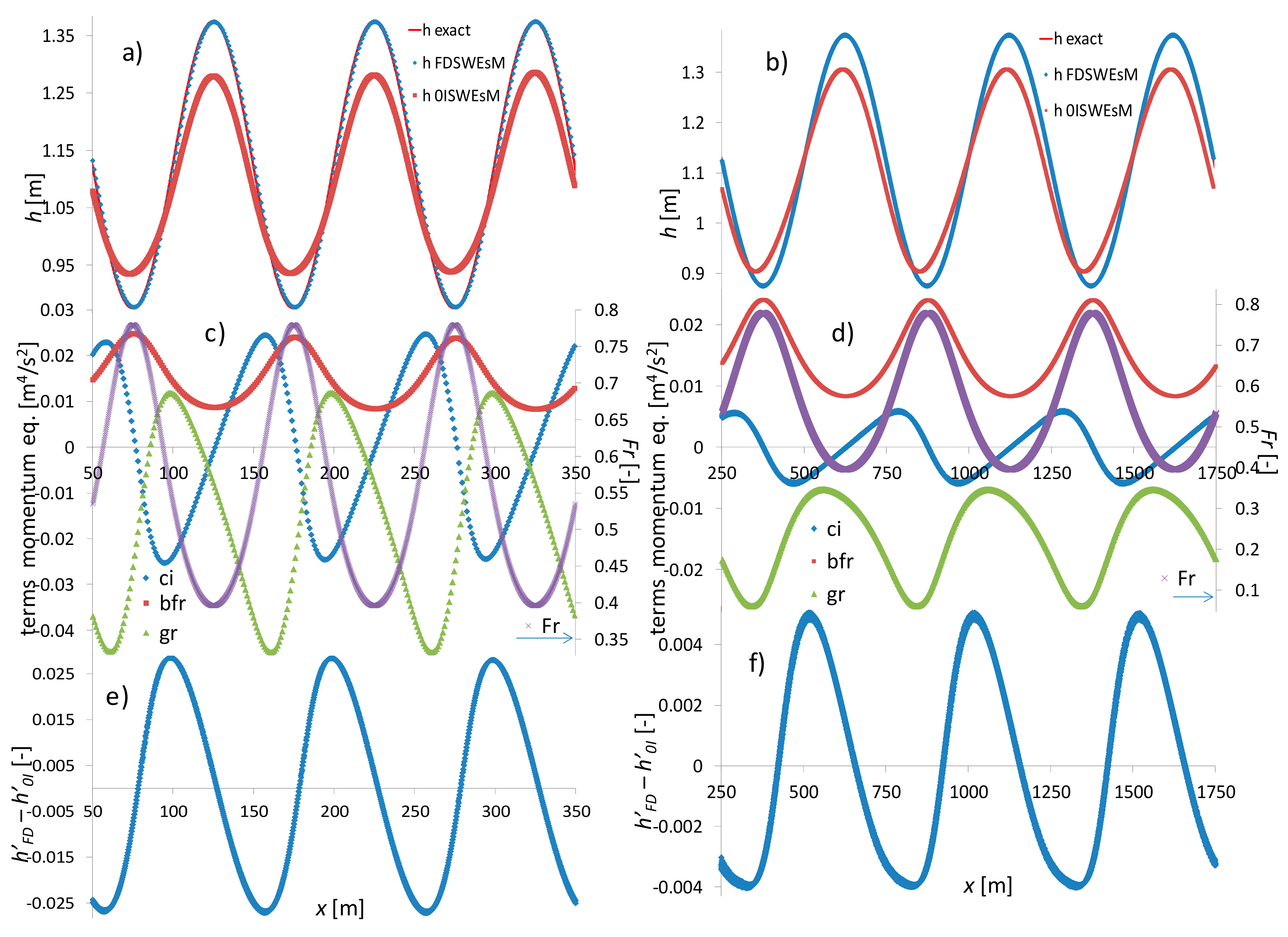
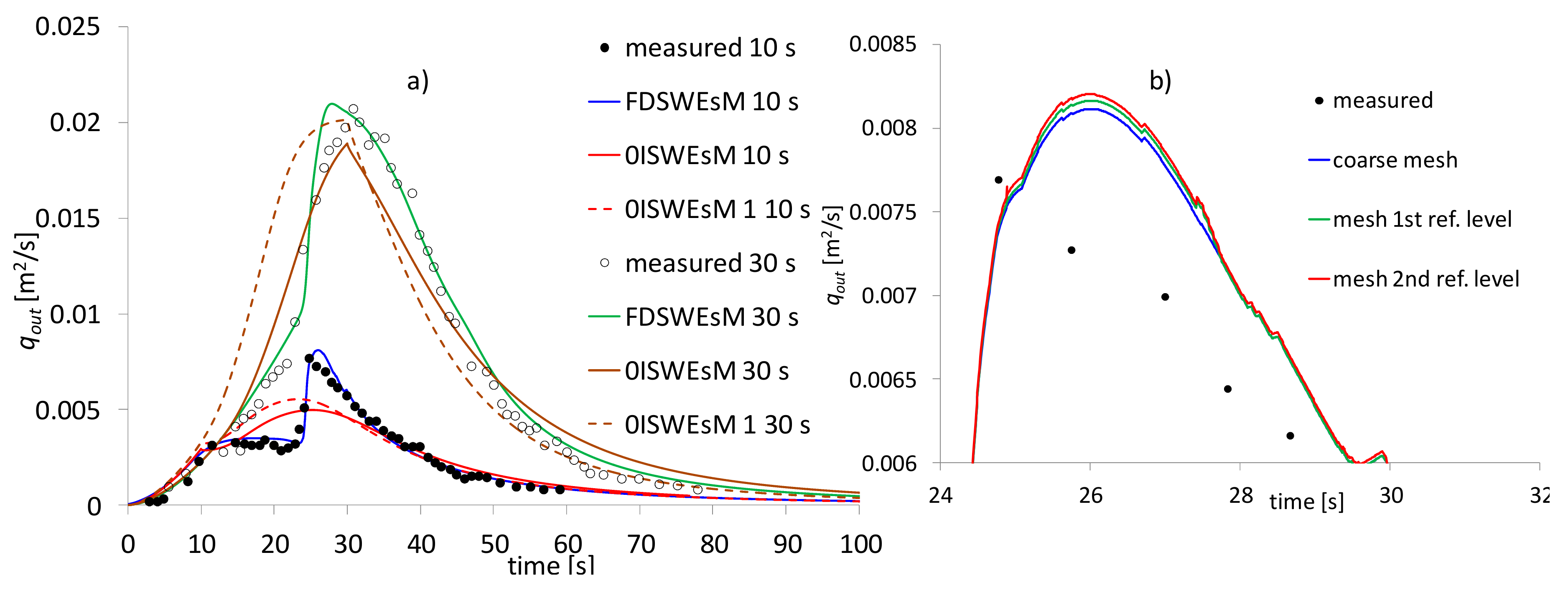
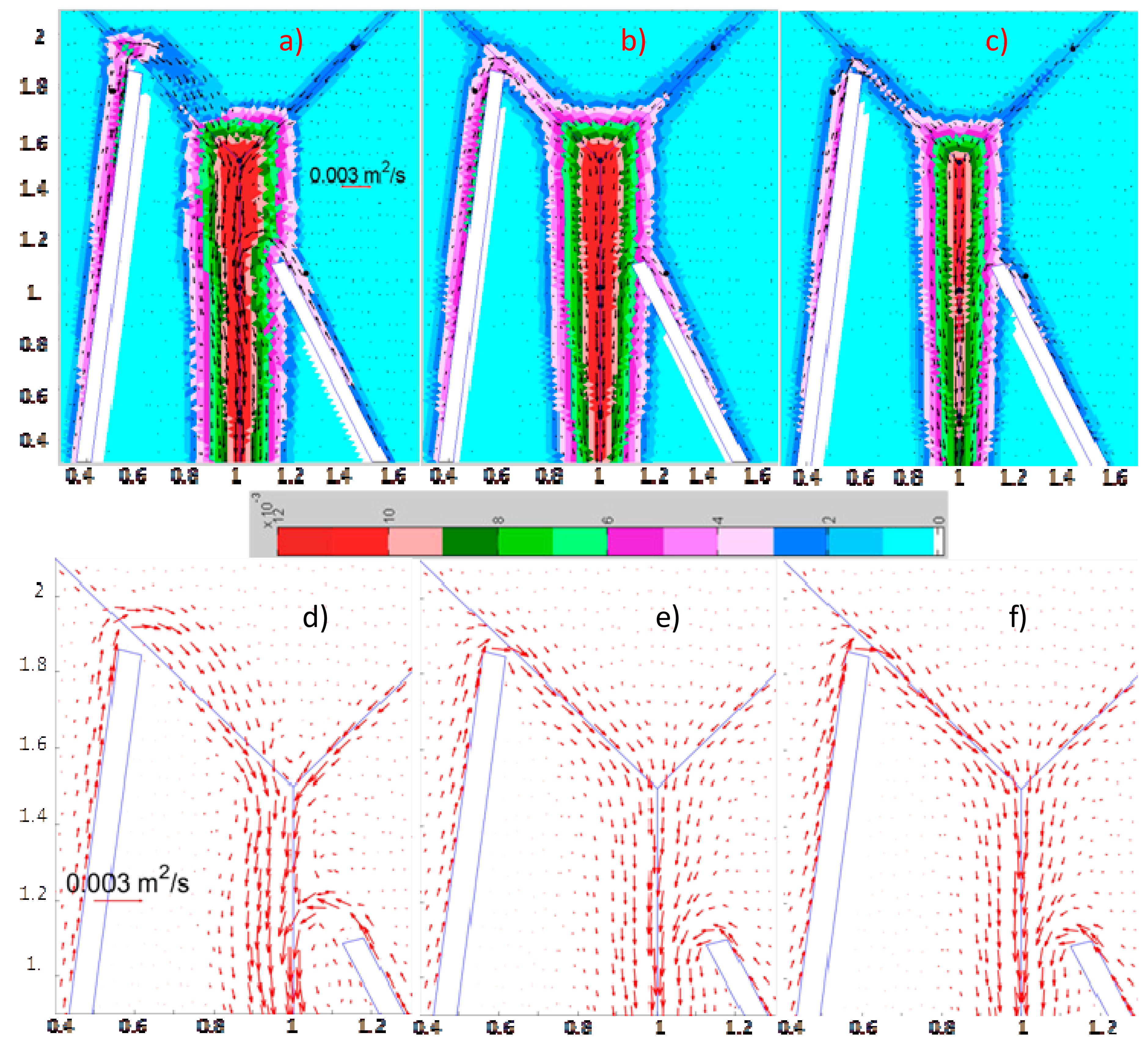
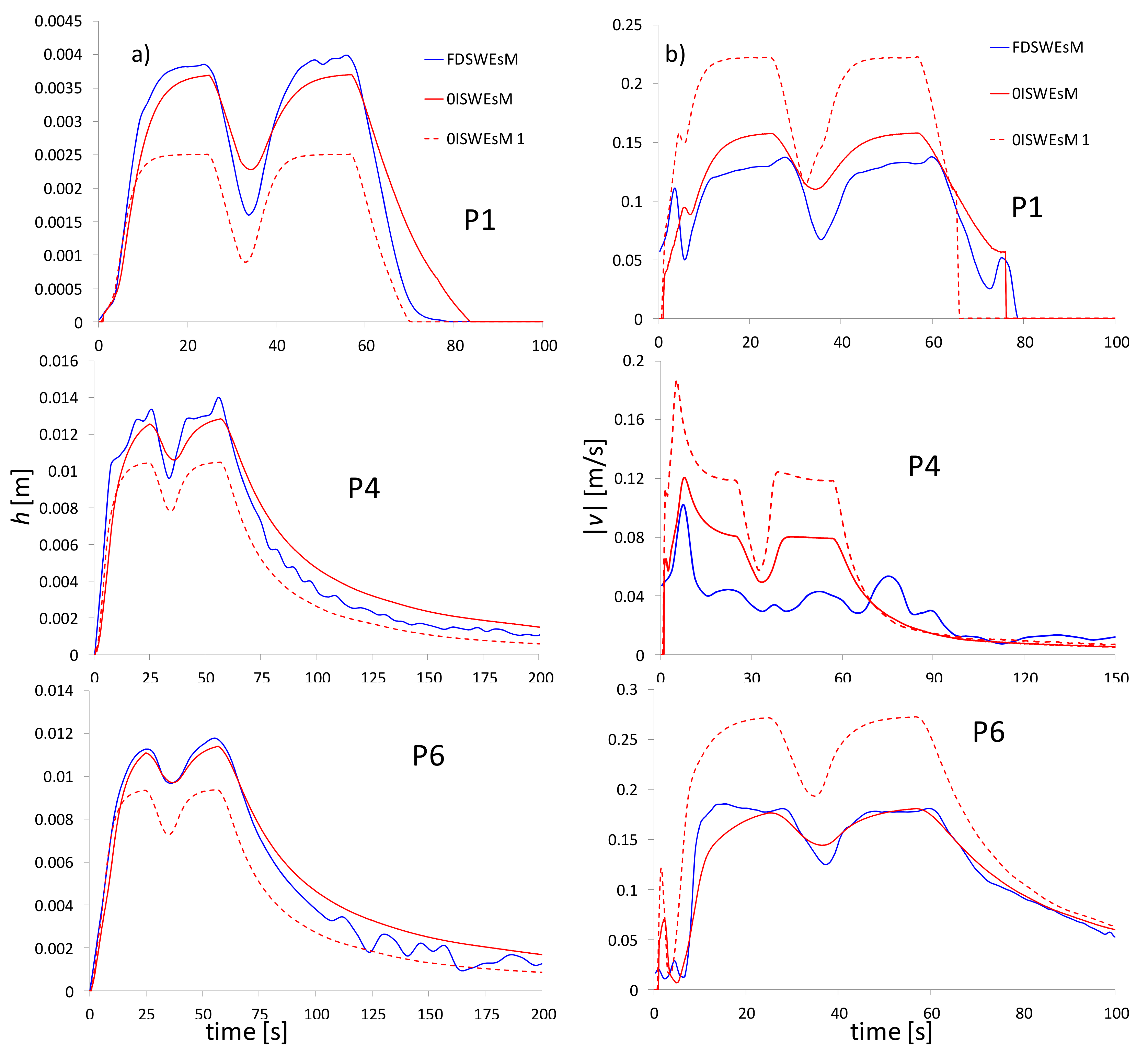
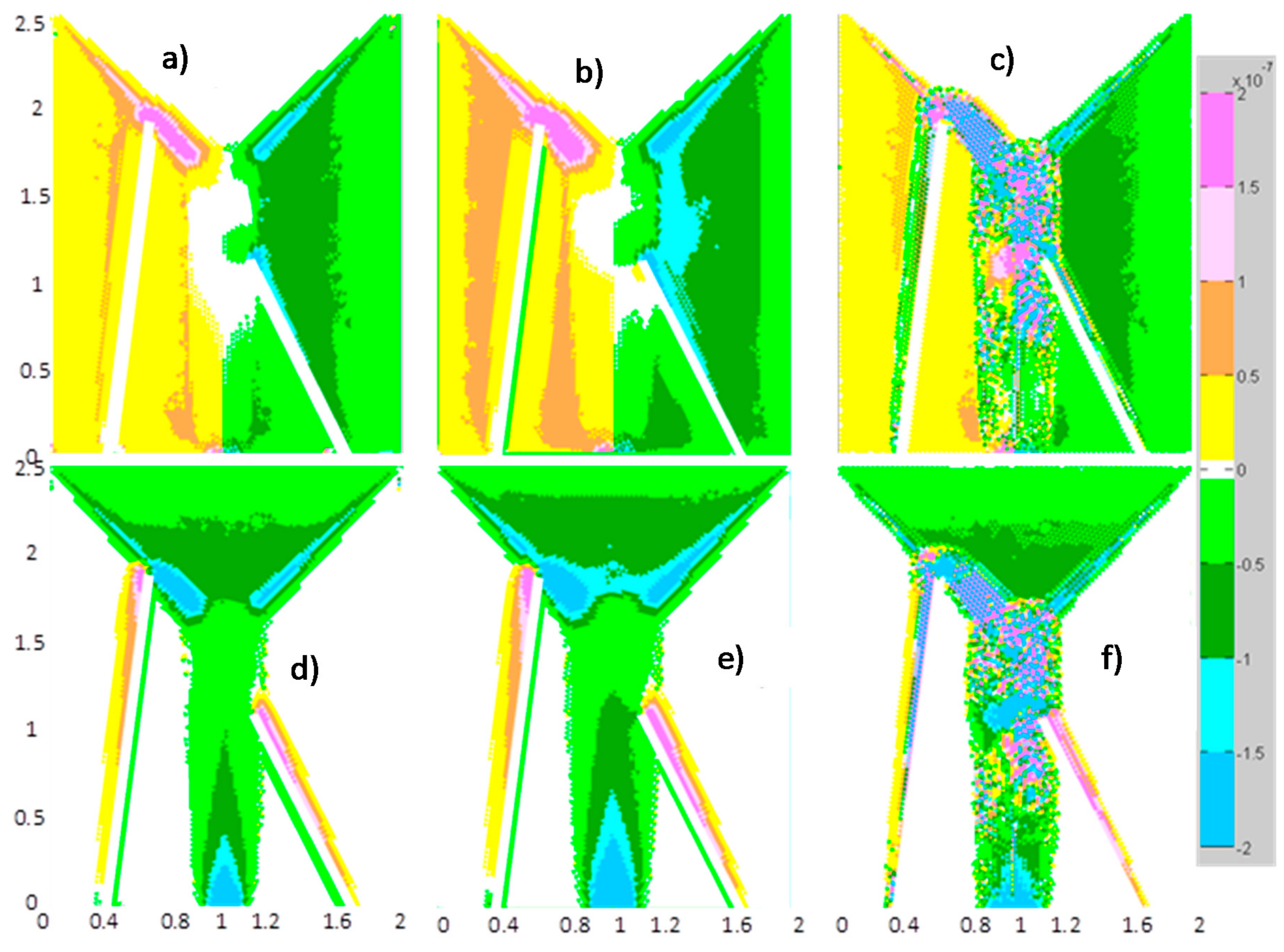
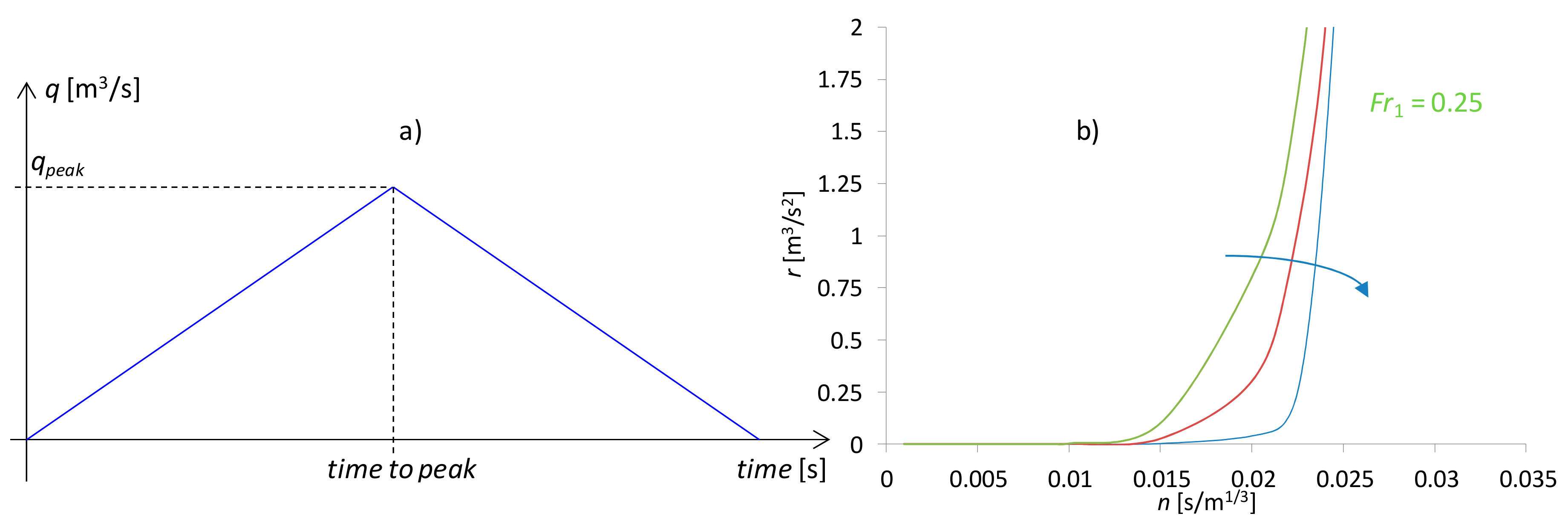
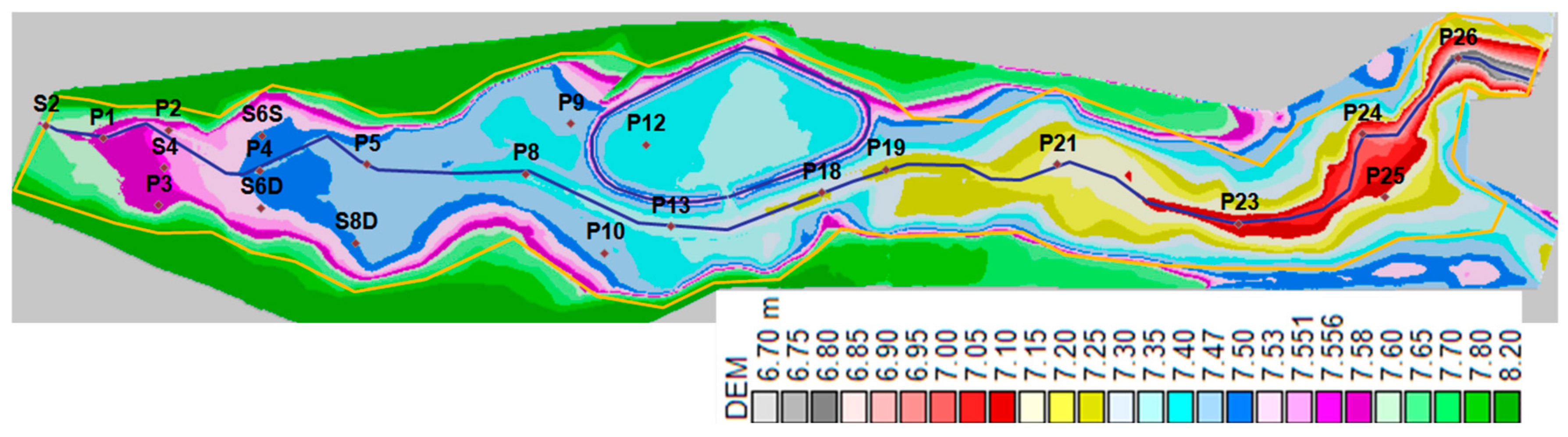
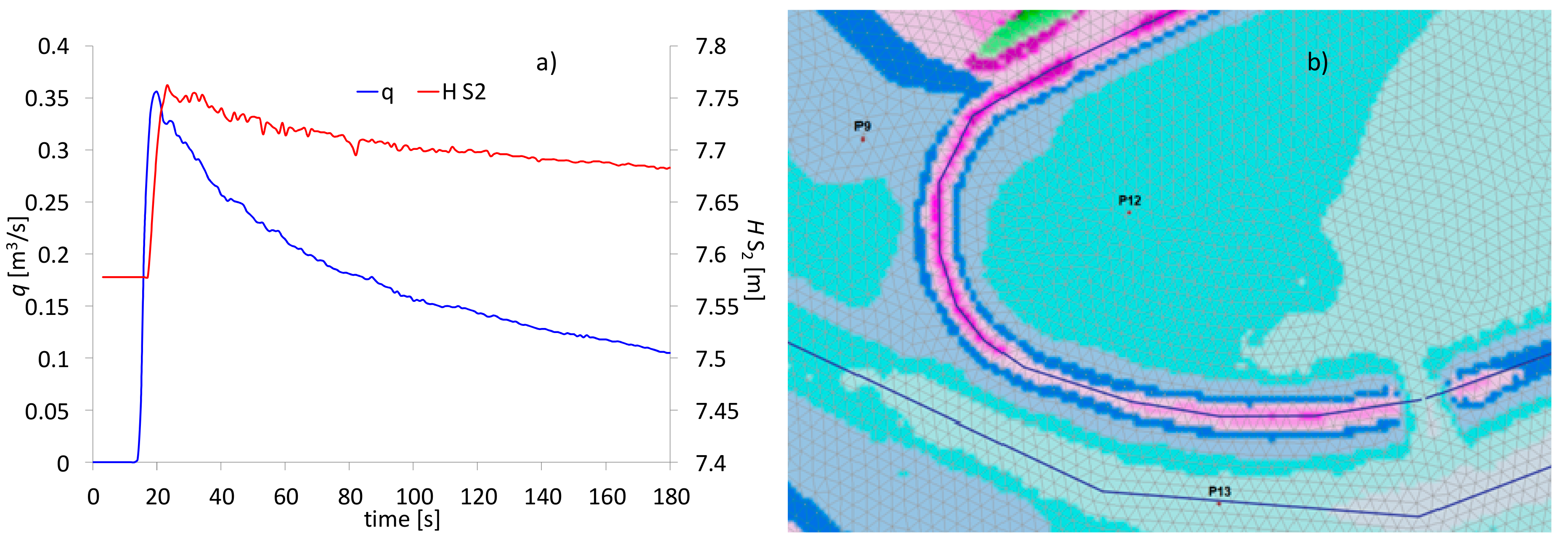
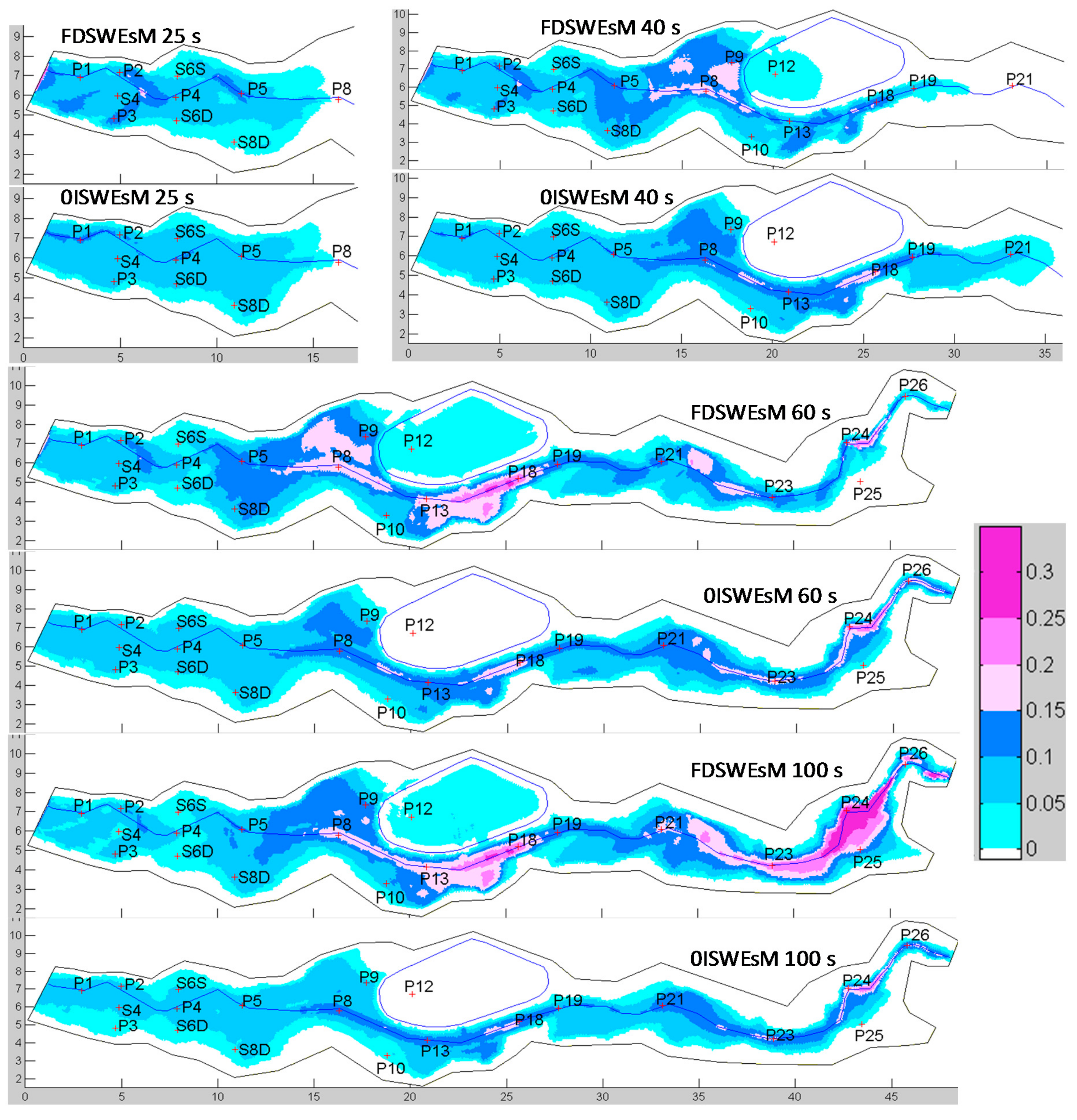
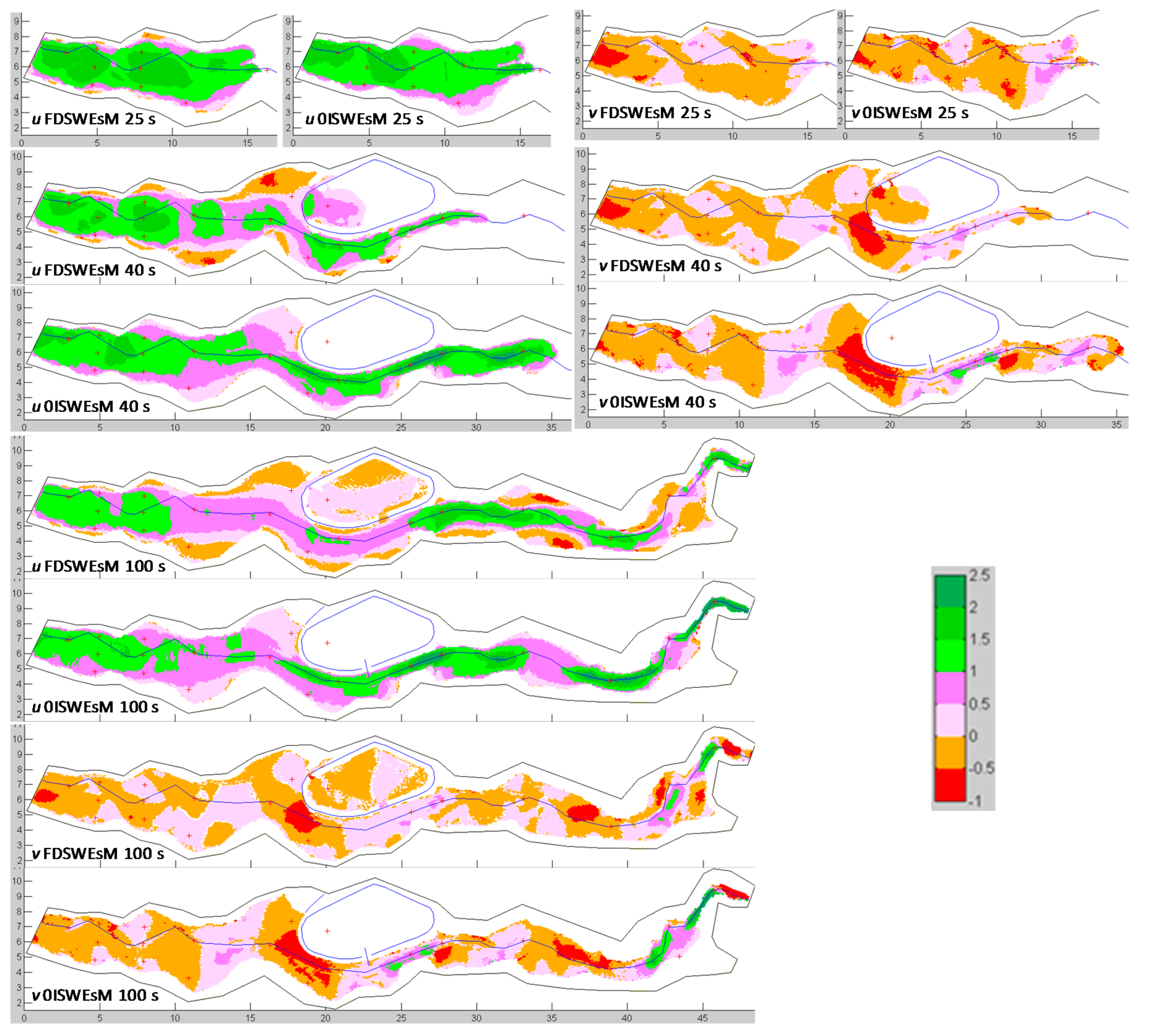
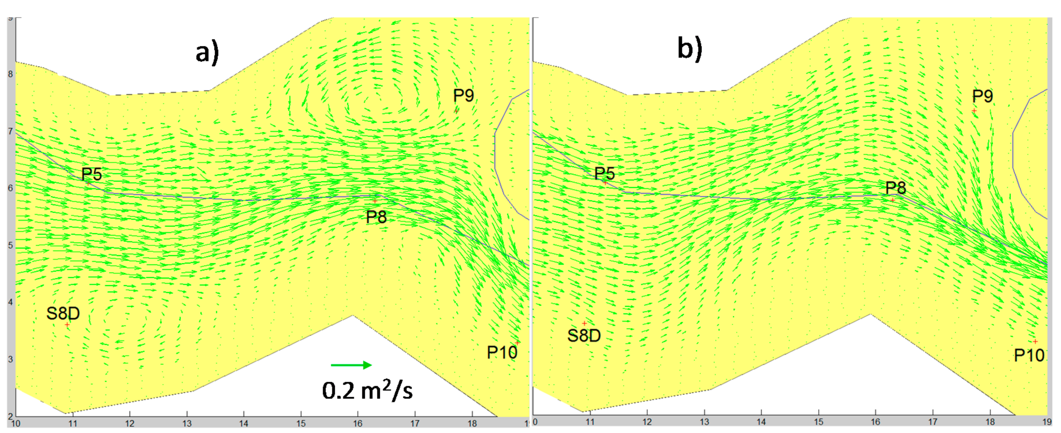
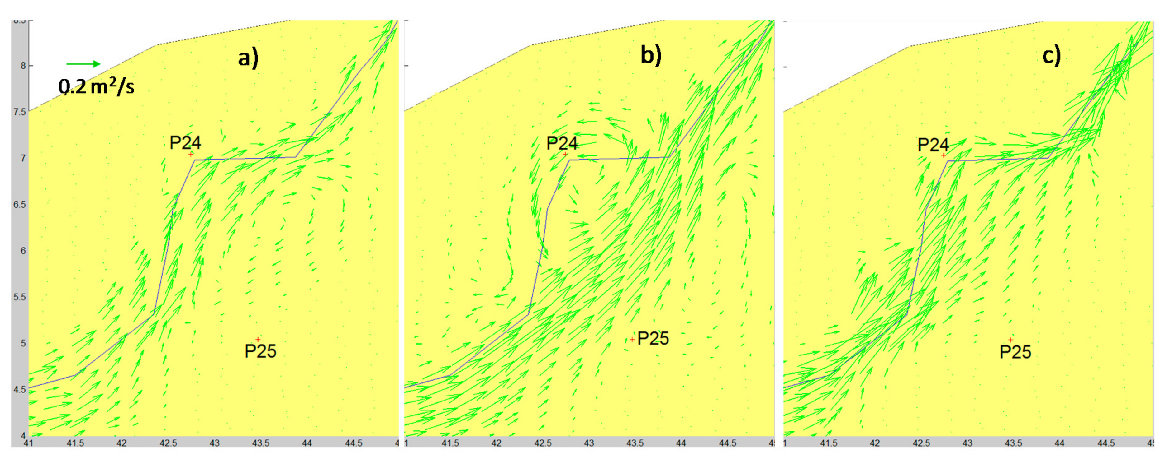
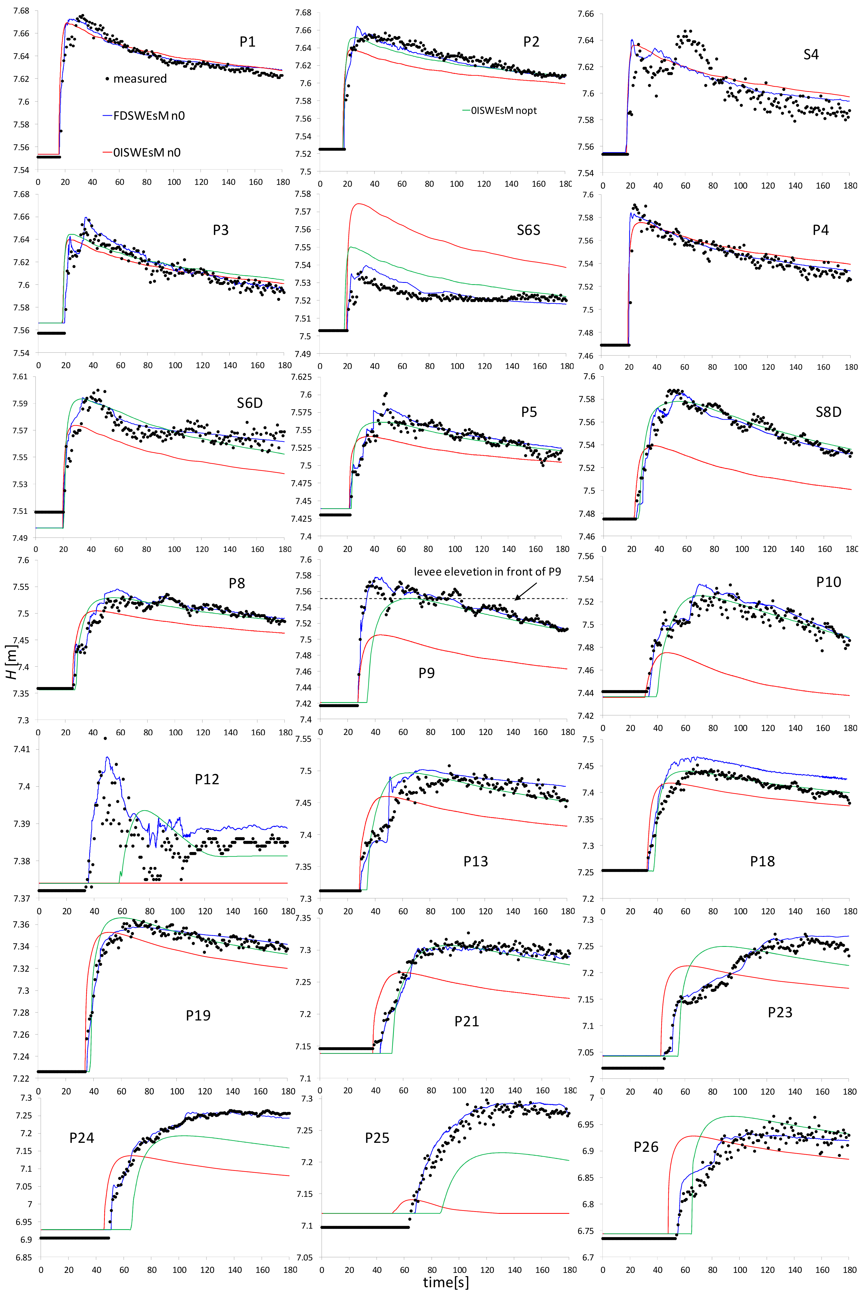
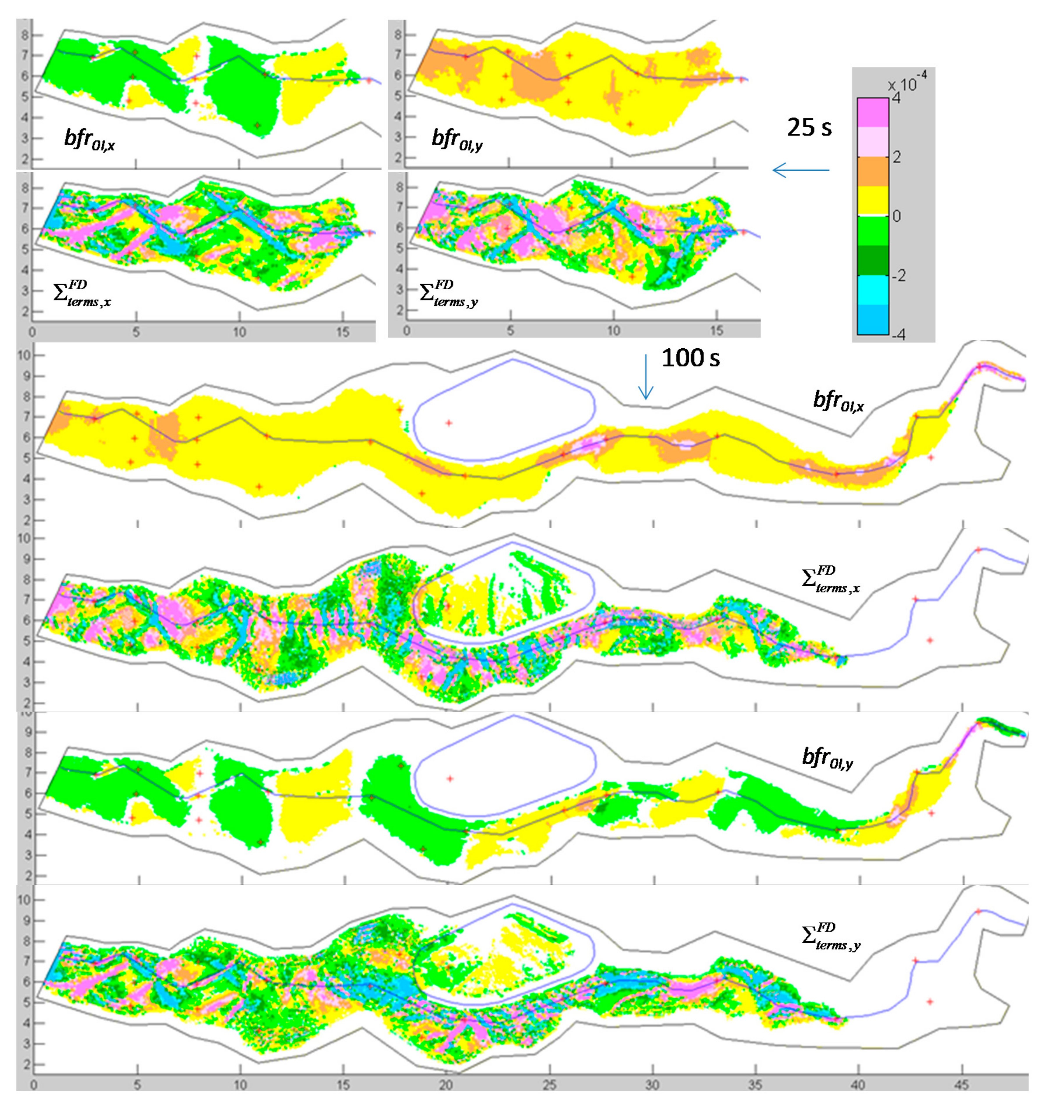
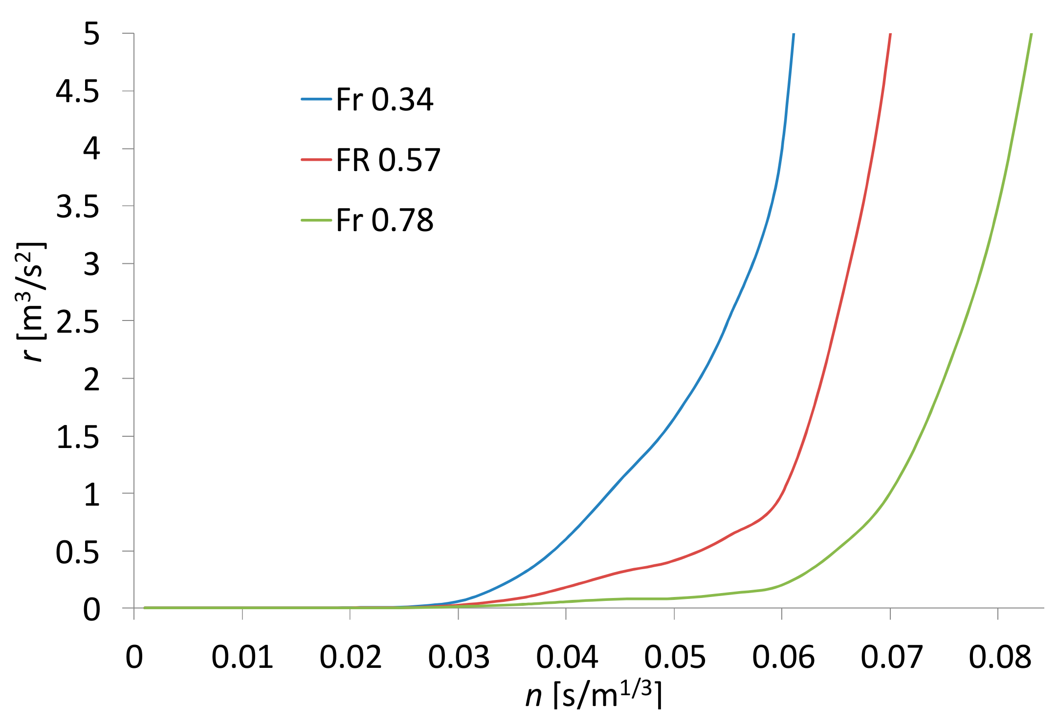
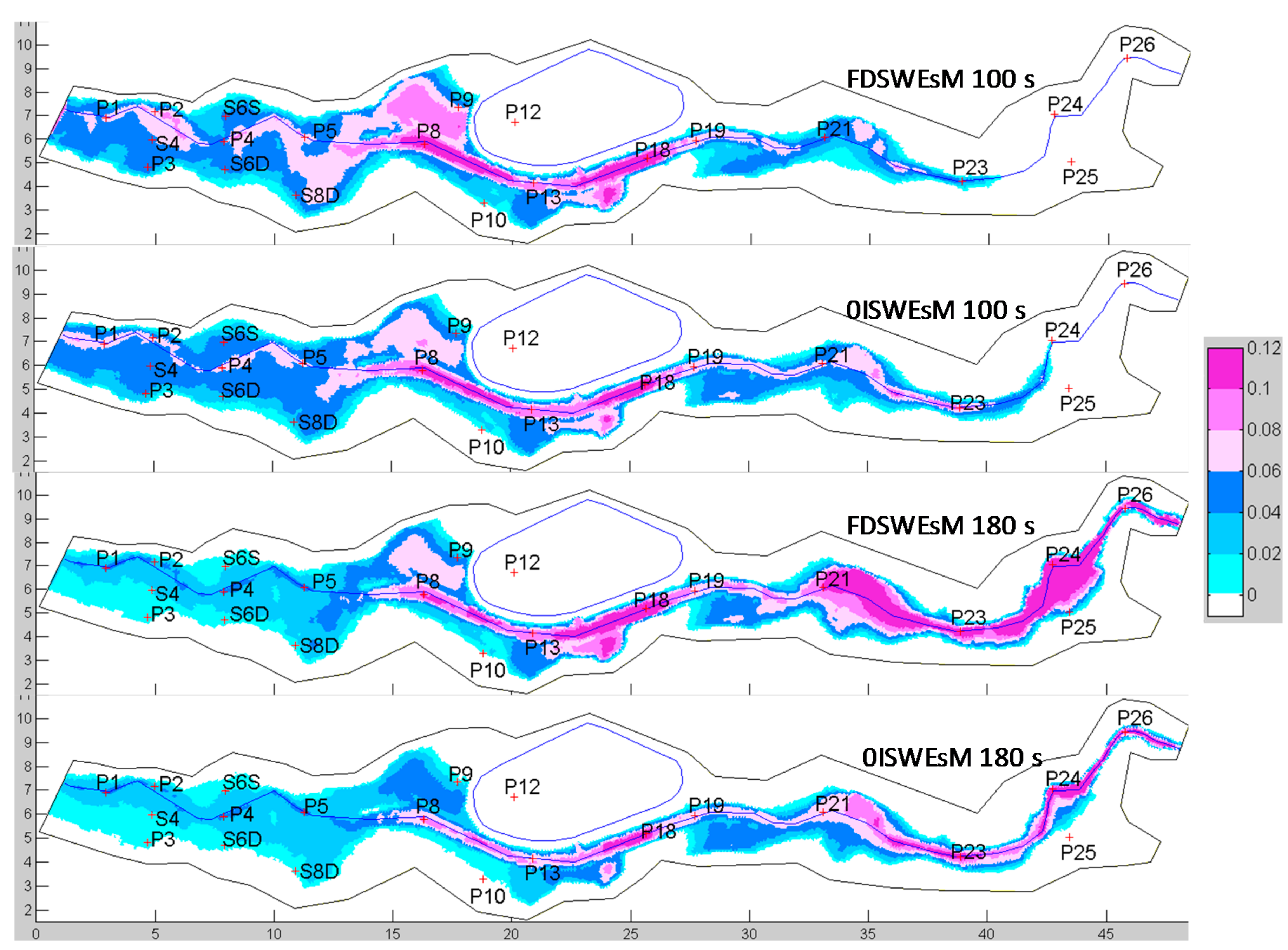
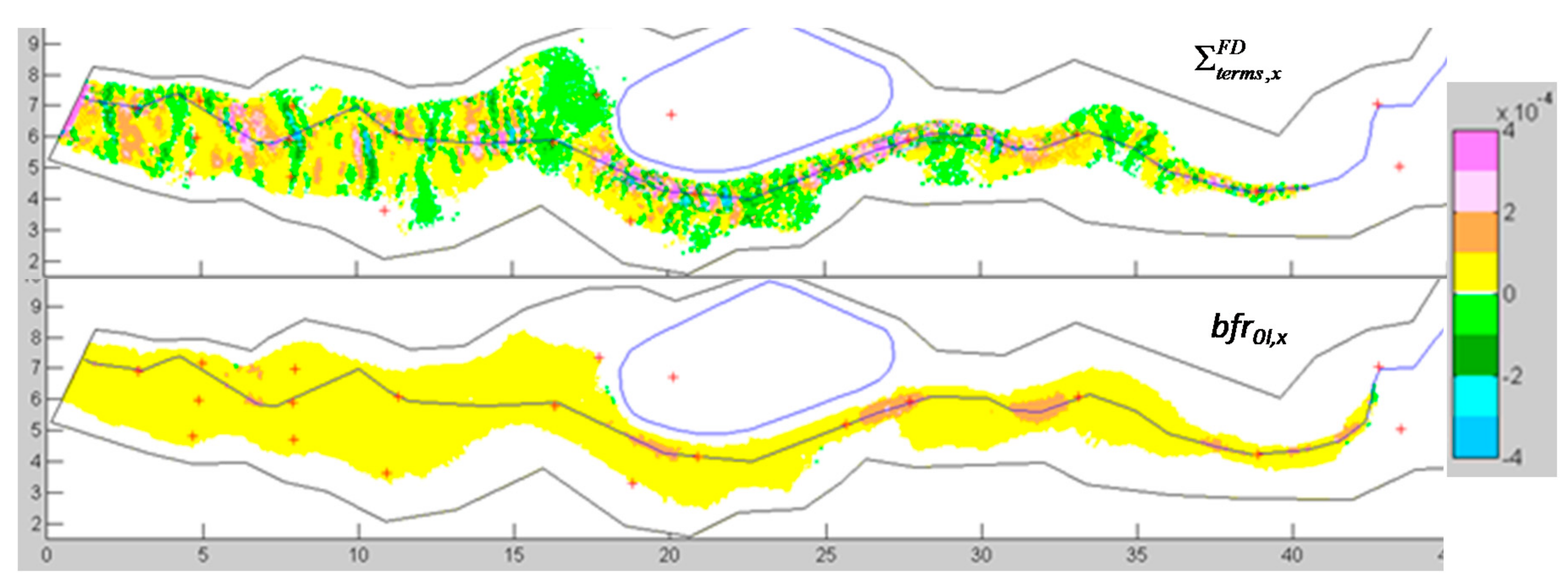
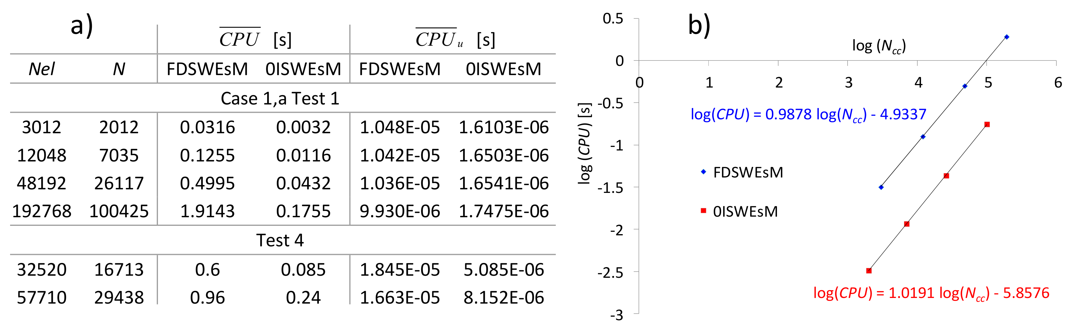
Table 1.
Test 1. L1 and L2 norms of the relative errors for h and uh of the 0ISWEsM. Unstructured mesh. (Abbreviations. L1(2),h are the L1(2) norms of h. L1(2), uh are the L1(2) norms of uh. rc is the convergence order).
Table 1.
Test 1. L1 and L2 norms of the relative errors for h and uh of the 0ISWEsM. Unstructured mesh. (Abbreviations. L1(2),h are the L1(2) norms of h. L1(2), uh are the L1(2) norms of uh. rc is the convergence order).
| rc | L1,h | rc | L1,uh | rc | L2,h | rc | L2,uh |
| case 1 | |||||||
| 0.323 | 0.0311 | 0.350 | 0.0031 | 0.384 | 0.0526 | 0.348 | 0.0053 |
| 0.520 | 0.0248 | 0.464 | 0.0024 | 0.481 | 0.0403 | 0.496 | 0.0042 |
| 0.615 | 0.0173 | 0.660 | 0.0017 | 0.597 | 0.0289 | 0.577 | 0.0030 |
| 0.0113 | 0.0011 | 0.019 | 0.0020 | ||||
| case 2 | |||||||
| 0.712 | 0.0070 | 0.502 | 0.0028 | 0.799 | 0.0126 | 0.476 | 0.0041 |
| 0.817 | 0.0043 | 0.634 | 0.0020 | 0.844 | 0.0073 | 0.694 | 0.0029 |
| 0.991 | 0.0024 | 0.876 | 0.0013 | 1.083 | 0.0040 | 0.807 | 0.0018 |
| 0.0012 | 0.0007 | 0.0019 | 0.0010 | ||||
Table 2.
Test 1. L1 and L2 norms of the relative errors for h and uh of the FDSWEsM. Unstructured mesh. (Abbreviations as for Table 1).
Table 2.
Test 1. L1 and L2 norms of the relative errors for h and uh of the FDSWEsM. Unstructured mesh. (Abbreviations as for Table 1).
| rc | L1,h | rc | L1,uh | rc | L2,h | rc | L2,uh |
| case 1 | |||||||
| 0.949 | 0.0036 | 0.987 | 0.0023 | 0.996 | 0.0059 | 0.907 | 0.0049 |
| 1.055 | 0.0019 | 1.059 | 0.0011 | 1.030 | 0.0030 | 0.927 | 0.0026 |
| 1.065 | 0.0009 | 1.026 | 0.0006 | 1.012 | 0.0015 | 1.077 | 0.0014 |
| 0.0004 | 0.0003 | 0.0007 | 0.0006 | ||||
| case 2 | |||||||
| 0.971 | 0.0036 | 0.994 | 0.0023 | 0.948 | 0.0060 | 0.963 | 0.0049 |
| 1.047 | 0.0019 | 1.089 | 0.0011 | 1.050 | 0.0031 | 1.048 | 0.0025 |
| 1.103 | 0.0009 | 1.030 | 0.0005 | 1.001 | 0.0015 | 1.007 | 0.0012 |
| 0.0004 | 0.0003 | 0.0007 | 0.0006 | ||||
Table 3.
Test 2. Characteristics of the experimental runs and of the lab flume.
| Case | Rain Duration (s) | Geometrical and Hydrological Data | Reach 1 (0–8 m) | Reach 2 (8–16 m) | Reach 3 (16–24 m) |
|---|---|---|---|---|---|
| 1 | 10 | slope channel (–) | 0.02 | 0.015 | 0.01 |
| 2 | 30 | rain intensity (mm/h) | 3890 | 2300 | 2880 |
| flow rate (m2/s) | 0.025933 | 0.015333 | 0.0192 |
Table 4.
Test 2. The computed nopt values which minimize the L1, L2 and Linf norms.
| Case | FDSWEsM | 0ISWEsM | ||||
|---|---|---|---|---|---|---|
| L1 | L2 | Linf | L1 | L2 | Linf | |
| 1 | 0.0090512 | 0.00905122 | 0.0090725 | 0.0112 | 0.01125 | 0.01125 |
| 2 | 0.0091203 | 0.009124 | 0.009214 | 0.01325 | 0.01326 | 0.01326 |
Table 5.
Test 4. Differences of the computed and measured arrival time of the wavefront at the gauges (left). nopt values for the two solvers which minimize the L1, L2 Linf norms of the relative errors at each gauge (right).
Table 5.
Test 4. Differences of the computed and measured arrival time of the wavefront at the gauges (left). nopt values for the two solvers which minimize the L1, L2 Linf norms of the relative errors at each gauge (right).
| Gauge | ∆t of the Arrival Time of the Front [s] | nopt Values [s/m1/3] Which Minimize the Norms | ||||||||
|---|---|---|---|---|---|---|---|---|---|---|
| FDSWEsM | 0ISWEsM | FDSWEsM | 0ISWEsM | |||||||
| n0 | nopt | n0 | nopt | L1 | L2 | Linf | L1 | L2 | Linf | |
| P1 | 0.01 | 0.01 | 0.01 | 0.01 | 0.016 | 0.0155 | 0.0142 | 0.016 | 0.015 | 0.014 |
| P2 | 0.01 | 0.01 | 0.02 | 0.02 | 0.0162 | 0.0161 | 0.0168 | 0.022 | 0.022 | 0.022 |
| P3 | 0.9 | 0.9 | 1.2 | 1.2 | 0.0161 | 0.0161 | 0.017 | 0.018 | 0.016 | 0.022 |
| S4 | 0.1 | 0.1 | 0.1 | 0.1 | 0.0164 | 0.0166 | 0.016 | 0.014 | 0.014 | 0.014 |
| P4 | 0.9 | 0.9 | 0.8 | 0.8 | 0.016 | 0.0162 | 0.016 | 0.016 | 0.016 | 0.016 |
| S6S | 0.01 | 0.01 | 1.4 | 2 | 0.016 | 0.0162 | 0.017 | 0.008 | 0.008 | 0.008 |
| S6D | 0.04 | 0.04 | 0.04 | 0.02 | 0.016 | 0.0161 | 0.0164 | 0.022 | 0.023 | 0.019 |
| P5 | 0.45 | 0.1 | 0.7 | 0.1 | 0.016 | 0.016 | 0.0163 | 0.028 | 0.029 | 0.032 |
| P8 | 0.2 | 0.1 | 0.5 | −0.8 | 0.0158 | 0.0165 | 0.0165 | 0.027 | 0.028 | 0.027 |
| S8D | −0.6 | −0.6 | 0.9 | −0.9 | 0.0159 | 0.0161 | 0.0164 | 0.035 | 0.035 | 0.035 |
| P9 | 0.01 | 0.01 | 0.01 | −16 | 0.016 | 0.0162 | 0.0167 | 0.04 | 0.039 | 0.017 |
| P10 | −1 | −1.1 | 0.5 | −7 | 0.016 | 0.0164 | 0.0163 | 0.038 | 0.039 | 0.03 |
| P12 | −1 | −1.1 | no | −22 | 0.016 | 0.0162 | 0.0165 | 0.04 | 0.04 | 0.038 |
| P13 | 0.6 | 0.4 | 0.8 | −5 | 0.01607 | 0.0162 | 0.0164 | 0.028 | 0.028 | 0.025 |
| P18 | −0.8 | −0.78 | 0.2 | −4 | 0.01602 | 0.0162 | 0.0161 | 0.025 | 0.025 | 0.022 |
| P19 | −0.9 | −0.92 | 0.8 | −2 | 0.01602 | 0.016 | 0.0161 | 0.022 | 0.022 | 0.022 |
| P21 | −6 | −6 | 0.02 | −14 | 0.016 | 0.0161 | 0.0162 | 0.031 | 0.031 | 0.028 |
| P23 | 0.1 | 0.11 | 3 | −10 | 0.0161 | 0.0162 | 0.0163 | 0.025 | 0.03 | 0.022 |
| P24 | −0.6 | −0.9 | 4 | −15 | 0.0165 | 0.0171 | 0.0163 | 0.027 | 0.031 | 0.025 |
| P25 | −2.3 | −3 | 14 | −21 | 0.0164 | 0.0168 | 0.0161 | 0.038 | 0.05 | 0.05 |
| P26 | −0.7 | −0.7 | 8 | −10 | 0.016 | 0.0161 | 0.016 | 0.033 | 0.032 | 0.035 |
© 2018 by the authors. Licensee MDPI, Basel, Switzerland. This article is an open access article distributed under the terms and conditions of the Creative Commons Attribution (CC BY) license (http://creativecommons.org/licenses/by/4.0/).
Share and Cite
MDPI and ACS Style
Aricò, C.; Nasello, C. Comparative Analyses between the Zero-Inertia and Fully Dynamic Models of the Shallow Water Equations for Unsteady Overland Flow Propagation. Water 2018, 10, 44. https://doi.org/10.3390/w10010044
AMA Style
Aricò C, Nasello C. Comparative Analyses between the Zero-Inertia and Fully Dynamic Models of the Shallow Water Equations for Unsteady Overland Flow Propagation. Water. 2018; 10(1):44. https://doi.org/10.3390/w10010044
Chicago/Turabian StyleAricò, Costanza, and Carmelo Nasello. 2018. "Comparative Analyses between the Zero-Inertia and Fully Dynamic Models of the Shallow Water Equations for Unsteady Overland Flow Propagation" Water 10, no. 1: 44. https://doi.org/10.3390/w10010044
Note that from the first issue of 2016, this journal uses article numbers instead of page numbers. See further details here.