Hydrological Modeling Approach Using Radar-Rainfall Ensemble and Multi-Runoff-Model Blending Technique


1
Department of Civil Engineering, Inha University, Incheon 22212, Korea
2
Department of Land, Water and Environment Research, Korea Institute of Civil Engineering and Building Technology(KICT), Goyang-Si 10223, Korea
3
Urban Disaster Prevention & Water Resource Research Center, Korea Research Institute for Human Settlement(KRIHS), Sejong-si 30147, Korea
*
Author to whom correspondence should be addressed.
Water 2019, 11(4), 850; https://doi.org/10.3390/w11040850
Submission received: 6 March 2019
/
Revised: 18 April 2019
/
Accepted: 19 April 2019
/
Published: 23 April 2019
(This article belongs to the Special Issue Hydrological and Hydro-Meteorological Extremes and Related Risk and Uncertainty)
Abstract
:The purpose of this study is to reduce the uncertainty in the generation of rainfall data and runoff simulations. We propose a blending technique using a rainfall ensemble and runoff simulation. To create rainfall ensembles, the probabilistic perturbation method was added to the deterministic raw radar rainfall data. Then, we used three rainfall-runoff models that use rainfall ensembles as input data to perform a runoff analysis: The tank model, storage function model, and streamflow synthesis and reservoir regulation model. The generated rainfall ensembles have increased uncertainty when the radar is underestimated, due to rainfall intensity and topographical effects. To confirm the uncertainty, 100 ensembles were created. The mean error between radar rainfall and ground rainfall was approximately 1.808–3.354 dBR. We derived a runoff hydrograph with greatly reduced uncertainty by applying the blending technique to the runoff simulation results and found that uncertainty is improved by more than 10%. The applicability of the method was confirmed by solving the problem of uncertainty in the use of rainfall radar data and runoff models.
1. Introduction
Climate changes caused by human activities are affecting the frequency and intensity of extreme weather phenomena and causing rises in temperature, changes in precipitation and precipitation patterns, and rising sea levels. In recent years, Korea has also suffered from frequent local storms and typhoons due to climate change [1,2]. It is necessary to predict rainfall and runoff accurately and many methods have been sought to reduce flood damage. It is especially important to minimize rainfall damage by assessing the reliability of rainfall with characteristics of high rainfall intensity in the short term, such as heavy rainfall. However, it is difficult to quantify and predict the characteristics of rainfall by measuring rainfall from a ground gauge because rainfall shows a wide range of spatiotemporal variability. Radar rainfall data can be used to predict and observe changes in rainfall in real time, but the data are estimates of rainfall based on indirect observations through the reflectivity from airborne bodies. Therefore, there are problems of accuracy and uncertainty.
Many studies related to the uncertainty of radar rainfall data have been conducted to solve these problems. Chiang et al. studied radar rainfall data correction and used a dynamic artificial neural network to estimate the quantitative precipitation (QPE) from radar data [3]. Seck at al. evaluated three geostatistical interpolation techniques, ordinary kriging (OK), conditional merging (CM), and kriging with an external drift (KED), to merge radar and rain gauge data at high temporal resolutions [4]. Adirosi et al. compared precipitation measurement algorithms, measured by drop size distributions (DSD), and evaluated the impact of the instrumental errors on these algorithms [5]. Kuriqi calibrated the radar data for the Grenoble region affected by altitude and geomorphology, and confirmed that the radar was undervalued and overestimated due to the screening and ground clutter effect [6]. Kang et al. performed radar rainfall corrections and compared them with ground rainfall data. They used the SWMM model to simulate runoff [7]. Kim et al. used the Kalman filter (KF) and low pass filter (LF) to remove noise from the radar data and the result showed that the KF was better than the LF, based on BDS (Brock–Dechert–Scheinkman) statistics [8,9]. BDS statistics can be applied to the estimated residuals of any time series model and used as a model selection tool.
One way to evaluate the spatiotemporal uncertainty of radar rainfall data is to generate rainfall ensembles that can occur. Germann et al. proposed a method in which an error field is added to radar observations to generate radar precipitation ensembles [10,11]. Dai et al. developed a rainfall estimation model that can quantify uncertainties in deterministic and random errors, based on the conditional distribution of errors in radar and ground rainfall data. This was achieved using the elliptical copula and Archimedean copula functions [12]. Kang et al. proposed a probabilistic method for expressing the uncertainty of radar rainfall data and applied it to a rainfall event to evaluate the applicability of a technique proposed to generate rainfall ensembles [13].
The uncertainty in runoff prediction has been studied extensively, but the uncertainty in runoff models has been relatively neglected, compared to the model structure and the parameter correction of each model. Bates and Granger applied economic concepts to hydrology to reduce the uncertainty of runoff results [14]. Al-Safi et al. used a conceptual lumped-parameter rainfall-runoff model (HBV model) to assess the impact of climate change and found that results show a noticeable reduction in the mean annual streamflow during the mid-century, particularly for the RCP4.5 relative to the current streamflow [15,16]. McLeod et al. first introduced combined forecasting, where multiple flow-forecasting models are weighted and combined, which is now recognized as the blending technique [17]. The blending technique is a method of reducing the uncertainty of models by combining several models to obtain improved prediction results, and its application is increasing [18,19]. Ajami et al. applied various blending techniques to the results of the international Distributed Model Intercomparison Project (DMIP), such as the simple multi-model average (SMA) technique, the multi-model super ensemble (MMSE) technique, the modified multi-model super ensemble (M3SE) technique, and the weighted average method (WAM). They compared and analyzed the results [20].
Previous studies attempted to solve the spatiotemporal errors of the radar, but converted radar rainfall could not be solved completely because of a large error in radar reflectivity. In order to use radar rainfall in the hydrology field, the uncertainty of rainfall should be expressed by generating possible rainfall ensembles that can reflect spatiotemporal errors. However, there are only a few studies on rainfall ensembles that can describe the uncertainty of rainfall. In the present study, we generated rainfall ensembles using a probabilistic method to express uncertainty of rainfall. The runoff analysis was performed using the three runoff models (the tank model, the SSARR model, and the storage function model) with rainfall ensembles as input data. Three blending techniques were applied to reduce uncertainty, and the optimal runoff hydrograph was obtained.
2. Methodology
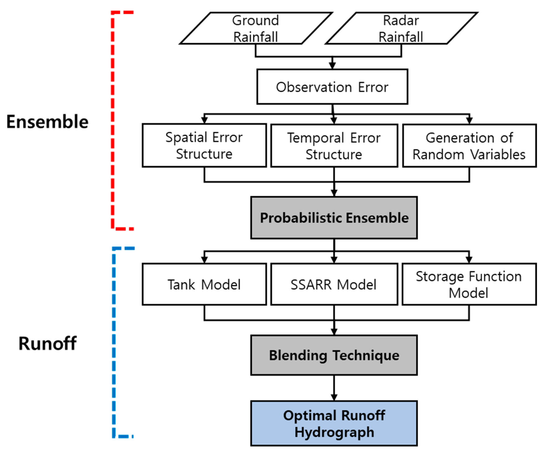
Figure 1 shows a diagram of the study. We created probabilistic rainfall ensembles using ground and radar data to determine the uncertainty because radar rainfall data have spatiotemporal errors. The generated rainfall ensembles were used as input data for three runoff models to perform a runoff analysis. The runoff results differ among runoff models, even though the same input data are used, because of the difference in model structures and assumptions of each runoff model. Therefore, we applied blending techniques to reduce the uncertainty and calculated the optimal runoff hydrograph.
2.1. Rainfall Ensemble Technique
A small value added to radar data is called a perturbation, and a combined field with perturbation is called a rainfall ensemble. The basic concept of applying ensembles to radar rainfall data is shown in Equation (1). The radar data calculated through the radar observation are deterministic, so it is possible to generate ensembles by adding uncertainty to the radar data. The combined field of the radar data () at time t with the ith perturbation () added is expressed as follows:
where:
- = the rainfall ensemble at time t (mm/h);
- = the radar data at time t (mm/h);
- = the ith perturbation generated at time t given the spatiotemporal errors of radar rainfall (mm/h);
- = the number of perturbations to be generated. More than 50 random numbers should be generated to show the uncertainty of the random error in the radar data [21].
The uncertainty () in radar data is based on the time–space error structure of the radar rainfall data. Given the amplification characteristics of uncertainty (), the observation errors between ground and radar data can be defined in units of decibels (dB), using Equation (2).
where:
- = the ratio of ground rainfall to radar rainfall, the observation error at time t (dBR);
- and = the rain-gauge rainfall and radar rainfall at time t expressed in units of rainfall intensity (mm/h).
Rain-gauge rainfall is a point value, while radar rainfall is an area value. Therefore, the grid value of the radar rainfall on location at the rain-gauge station is used when calculating the residual, using Equation (2). It is necessary to simulate the spatiotemporal error of the rainfall to generate rainfall ensembles. To this end, spatial and temporal correlation coefficients were applied in order to model the error structure of radar rainfall data. First, Equation (2) is used to calculate the observation error of the radar and ground rainfall data, and then the mean error is calculated using Equations (3) and (4) to reflect the weights at corresponding times. Weighting is necessary to avoid irrelevant samples erroneously having large influence. By setting the weight to the observed precipitation like , we force the expected value of the ensemble for a given location to be equal to the original unperturbed component at that location [9]. The weight is the ratio of the radar rainfall during the time tth step to the cumulative radar rainfall at location k.
where:
- k = the location of the observation station in the watershed;
- = the number of time step;
- = the location of the radar grid corresponding to observation point k;
- = the observation error at k and time t (dBR);
- = the weight of observation error at k and time t (dBR);
- = the mean error at observation point k (dBR).
The covariance was estimated using the calculated mean error. The covariance among the observation points refers to the spatial variability, which is also used in the process of estimating temporal errors. The diagonal matrix of the covariance matrix is easily estimated using Equation (4), and the spatial covariance is estimated using Equation (5).
where:
- = the variance at point k;
- = the covariance between point k and l;
- = the number of time step.
For a number of rainfall observing stations n, the covariance matrix has a dimension of . The temporal correlation coefficient is calculated using Equations (6) and (7) with the mean error () and the weighted rainfall covariance () to consider the temporal correlation.
where:
● , = the time lag correlation coefficient (lag 1, 2) at point k.
The rainfall ensemble must reflect the spatial and temporal error of the rainfall. So, it is necessary to generate correlated random numbers. The covariance representing spatial correlation can be decomposed into a lower triangular matrix (L) by the Cholesky decomposition algorithm. The Cholesky decomposition method is used to generate two or more correlated random numbers. In the case of a symmetric matrix (C), a lower triangular matrix can be used, such as Equation (8).
where:
- = Symmetric matrix;
- = Lower triangular matrix.
The resulting covariance is decomposed into a lower triangular matrix (L) by the Cholesky decomposition, and the perturbation () is expressed as multiplying L by a random number and adding the mean error (see Equation (9)). The resulting perturbation () is applied to Equation (1) to generate radar rainfall ensembles.
where:
- = the mean error calculated by the kriging interpolation technique using (dBR);
- = the random number range from 0 to 1 allocated for the generation of ensembles, which is randomly generated values to represent uncertainty.
However, Equation (9) is a time-independent perturbation value and it is necessary to consider temporal correlation, depending on characteristics of continuous rainfall. Dai et al. confirmed that uncertainty of radar rainfall is related to the time correlation coefficient of less than three hours [22]. By combining the parameters of the AR(2) model, estimated by Priestley with Equation (9), it is possible to estimate the perturbation reflecting the spatial and temporal correlation like Equation (10) [9].
where:
- = perturbation field having autocorrelation and the perturbation at time (t−1) and (t−2) (mm/h);
- = parameters estimated by Yule–Walker equations. can be estimated using the time delay correlation coefficient () at point k;
- = rescaling factor calculated as the square root of the variance of the AR(2) model.
2.2. Multiple-Runoff Model
2.2.1. Tank Model
The tank model is a conceptual rainfall runoff model developed by Sugawara in 1961 [23]. The groundwater layer structure is modeled with tanks in the vertical direction to represent a watershed and perform a runoff analysis [24]. The tank models are intended to simulate either flood events or long-term runoff from a watershed, which is simulated by a combination of storage vessels. These models are mostly classified as deterministic, lumped, linear, continuous, and time-invariant models [25]. Tank models have the advantage of being applicable in places with insufficient observation data or watersheds where observation is difficult. The model structure is simple, and a small number of input data and parameters are required for runoff analysis.
2.2.2. SSARR Model
The streamflow synthesis and reservoir regulation (SSARR) model was developed in 1956 by the U.S. Corps of Engineers for the planning, design, and operation of water resource management [26]. The basic tracking equation adopted in the model is the storage equation, which is a continuity equation that is normally used for basins, watersheds, or reservoirs:
where:
- = the quantities of inflow and outflow at random time t ();
- = the quantity of storage ();
- = the storage constant.
Equation (14) is rewritten as the relationship between two random points, as Equation (15):
The subscripts 1 and 2 denote the starting and ending points, respectively, is the average inflow during , and is the computingtime interval. When applying Equation (14) to Equation (15), Equation (16) is obtained as a tracking equation:
The flow rate can be calculated by repeating the calculation process with the flow rate calculated in Equation (16) as the next starting flow rate.
2.2.3. Storage Function Model
The storage function model (SFM) is a flood runoff model developed by Kimura in 1961 for mountainous watersheds [27]. The flood discharge occurring in the natural state is an unsteady flow that changes very slowly. The storage function model can be interpreted with these characteristics. The nonlinearity characteristic of flood runoff can be fully considered.
The storage function model classifies the watershed into three conceptual areas according to the runoff characteristics: The runoff area, the infiltration area, and the percolation area. The runoff area is an impervious area that contributes to the runoff of rainfall from an early stage. The infiltration area contributes to the runoff after a certain amount of soil saturation occurs, following the infiltration of the rainfall into the surface. Finally, the percolation area is where rainfall runs off into the subsurface without directly contributing to river runoff. The watershed runoff and the channel runoff for the storage function model are estimated by Equations (17) and (18), respectively.
where:
- A = the area of the target watershed ();
- = the quantity of channel inflow ();
- = the quantity of channel outflow ().
2.3. Blending Technique
2.3.1. Multi-Model Super Ensemble (MMSE)
Many blending techniques have been proposed for the combination of multiple models, such as the use of simple or weighted averages for the predicted values of the model, multiple linear regression analysis, and Bayesian model averaging. The multi-model super ensemble (MMSE) technique is one of the common multi-model prediction methods in weather forecasting [28]:
where:
- = the multi-model prediction value at time t ();
- = the flow of the ith model at time t ();
- = the mean flow of the ith model at time t ();
- = the mean observed value ();
- = the regression coefficient of each model of the N number of models, which can be obtained by regression analysis.
2.3.2. Simple Model Average (SMA)
The SMA technique is a multi-model ensemble method proposed by Georgakaos in 2004 [18]. The SMA technique evaluates the ensemble runoff simulation, based on mean value analysis. The mean value of each model is obtained and compared at each time:
where:
- = the multi-model prediction value at time t obtained by the SMA equation ();
- = the mean observation value during the observation period ();
- = the flow of the ith model at time t ();
- = the mean flow of the ith model during the entire period ().
2.3.3. Mean Squared Error (MSE)
The mean squared error (MSE) technique uses simulated runoff and the mean squared errors of each model to obtain the overall MSE and applies it as a weight to present runoff curves of multiple models into a single integrated runoff curve. In other words, the MSE technique calculates a single integrated runoff curve by using weights obtained from the correction of a single model, based on its performance, and then combining multiple models:
where:
- = the observed flow at time t ();
- = the flow of the ith model at time t ();
- MSE = the mean square error of the ith model, calculated using .
The lower the MSE value, the higher the accuracy of the model is. Therefore, the reciprocal of the MSE value was taken like Equation (22), and the model with higher performance was assigned a higher weight. By multiplying and adding the simulated runoff of each model by the weight obtained from Equation (22), the integrated multi-model estimation () in Equation (23) is obtained.
3. Result and Discussion
3.1. Study Area and Data Collection
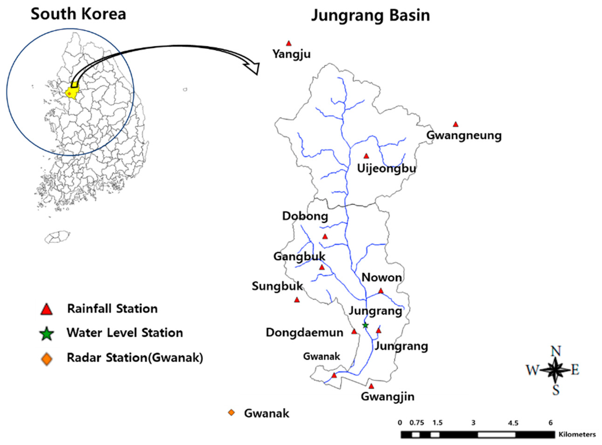
The Jungrang Basin is located in the central metropolitan area of the Korean Peninsula and was selected as the target watershed. Jungrang Basin is located in the lower part of the Han River, and there are many rainfall stations. Thus, it is easy to compare the rainfall data of stations with the radar rainfall data and generate ensembles. The watershed area of Jungrang Basin is 299.60 km2 and the watershed length is 32.80 km. The average width and altitude of the watershed are 8.1 km and EL. 107.2 m, respectively. Jungrang Basin is next to a major urban river and a highly populated area with a high potential risk of flooding.
Figure 2 shows the watershed of Jungrang River, the rainfall stations, and the river. The rainfall stations in Jungrang Basin include Uijeongbu, Dobong, Gangbuk, Nowon, and Jungrang. Rainfall data from five rainfall stations near Jungrang Basin were collected to take into account the spatial continuity of radar rainfall data. For the radar data, we used S-band radar data from the Gwanak Mountain station, which is operated by the Korea Meteorological Administration. They cover radii of 240.25 km (KWK) and record volume scans of reflectivity and Doppler velocity. The volume scan of the KWK radar includes observations at 12 elevation angles (0°, 0.4°, 0.8°, 1.2°, 1.6°, 2.0°, 3.0°, 4.2°, 5.7°, 7.5°, 9.8°, 12.5°). The correction of radar data was performed using the self-consistency of dual polarization parameters to convert the parameters that are not affected by the system error to the reflectivity [29,30]. The KNU-HSR method developed by Kyungpook National University was used for rainfall estimation. KNU-HSR is a method to improve the accuracy of rainfall estimation by using rainfall echo of the nearest radar bin without being affected by topographic echo and beam shielding [31]. In this study, the reflectivity–rainfall intensity (Z–R) relationship used for rainfall estimation is , and the rainfall intensity can be expressed as Equation (24).
where:
- = the rainfall intensity (mm/h), estimated using the reflectivity (Z, mm6/m)
The rainfall events and rainfall station sites are shown in Table 1. Both radar and ground rainfall data were collected at 10-min intervals at the point of rainfall observations.
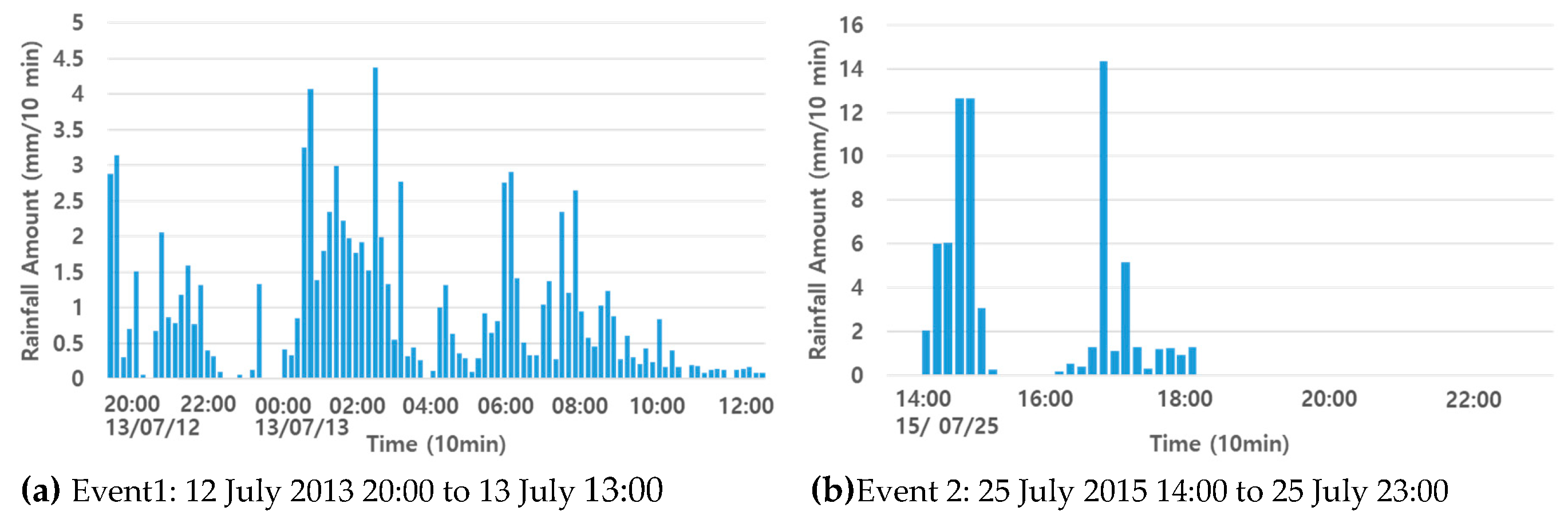
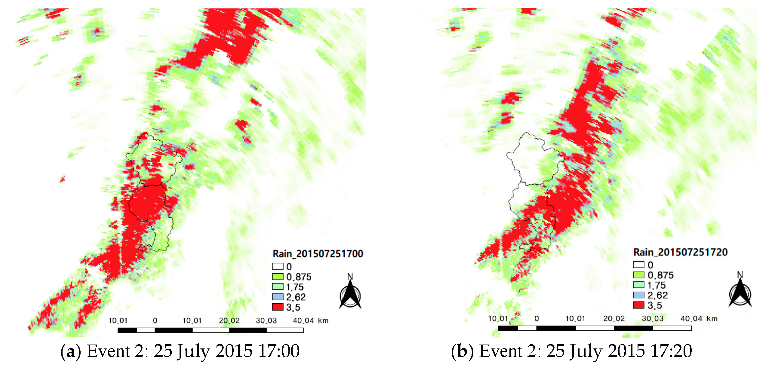
Accumulated rainfall for each rainfall event is shown in Figure 3. Event 1 shows a continuous rainfall pattern with a low intensity of less than 5 mm and Event 2 shows a rainfall pattern with a high intensity of more than 10 mm in a short time. Figure 4 shows the movement of rainfall in the northeast direction. In the case of localized rainfall, such as Event 2, the ground observation station can’t know the spatiotemporal characteristics of rainfall and the radar has the disadvantage of underestimating the rainfall. Therefore, in this study, we try to know the spatiotemporal characteristics of rainfall by generating a rainfall ensemble.
3.2. Generation of Rainfall Ensemble
The spatial error of radar rainfall data consists of the mean error and a covariance matrix. Using the methods described in Section 2.1, the observation error was estimated using the difference between the rainfall intensities of ground rainfall gauges and radar. In order to calculate the observation error, a true value must exist but there is no standard for this. In this study, the observation error was estimated with the assumption that the ground rainfall is the true value. Since the observation error is estimated based on the ground rainfall, the runoff obtained using the generated ensemble can express the uncertainty based on the runoff obtained using the ground rainfall.
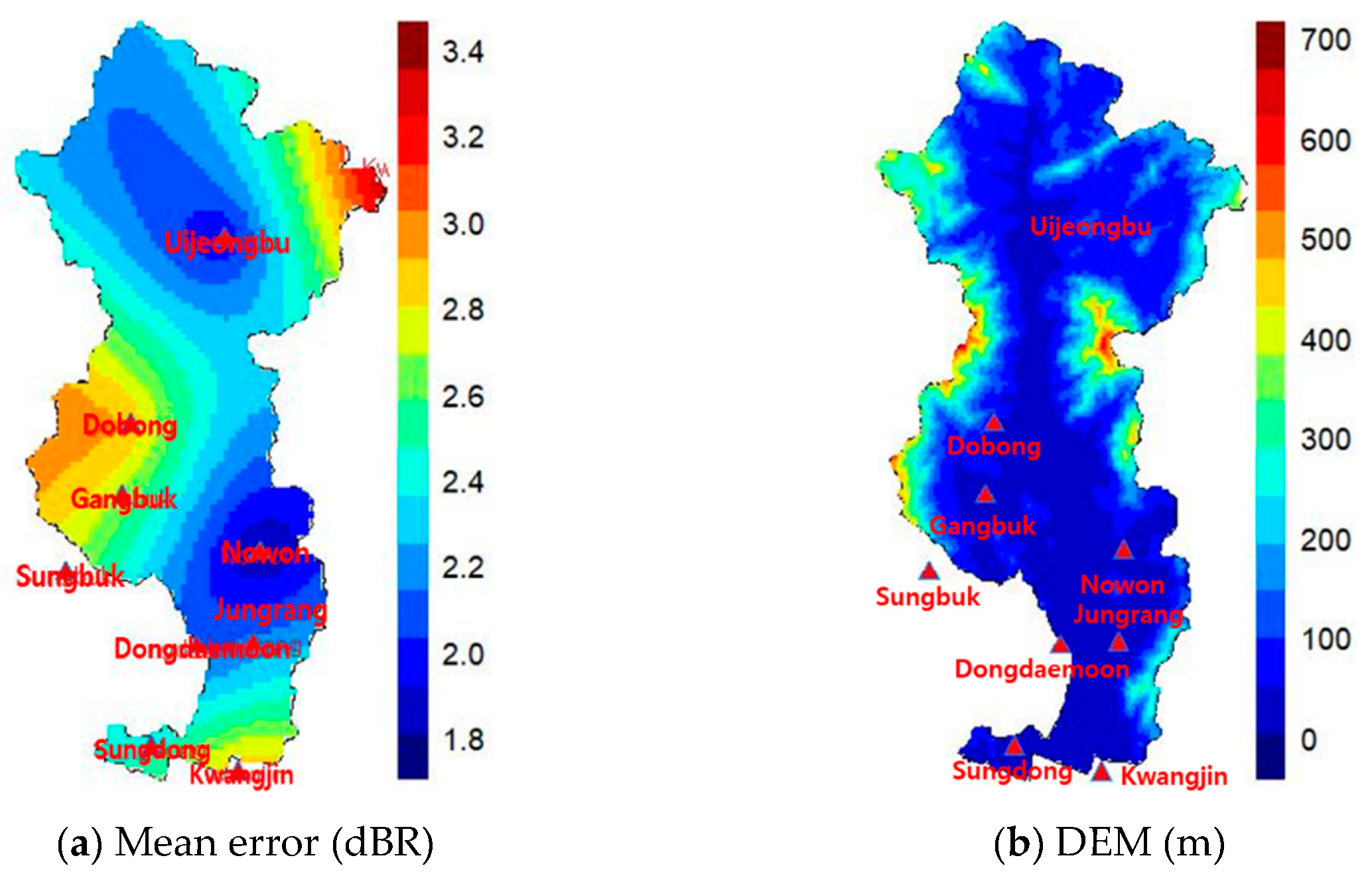
An interpolation method should be used for spatial distribution because the mean error obtained by Equation (3) is a point value. Ordinary kriging, which minimizes the error variance without bias of the kriging estimation equation, is used for the spatial distribution of the mean error. Figure 5a shows the result of the interpolation, using the mean error at each station. If the mean error is larger than 0, the radar rainfall is underestimated compared with the ground rainfall. If it is smaller than 0, the radar rainfall is overestimated.
The mean errors of observation stations are in the range of 1.808–3.354 dBR, and the radar rainfall is underestimated at all observation points. In particular, relatively large observation errors exceeding 2.7 dBR were calculated at the Uijeongbu, Dobong, and Sungbuk observation stations. When comparing these stations with the digital elevation models (DEM) of Jungrang Basin (Figure 5b), the observation errors were high in high-altitude areas. At low-altitude sites along the stream (Gangbuk, Nowon, and Jungrang), the observation error was relatively low (less than 2.2 dBR). Dobong and Gangbuk observation stations have a low altitude, but there are more than 500 m of mountain area on the left side. As a result, the radar rainfall was underestimated and the mean error was estimated to be relatively high at about 2.93 dBR. It was considered that the radar rainfall underestimated the actual rainfall due to the mountain effect.
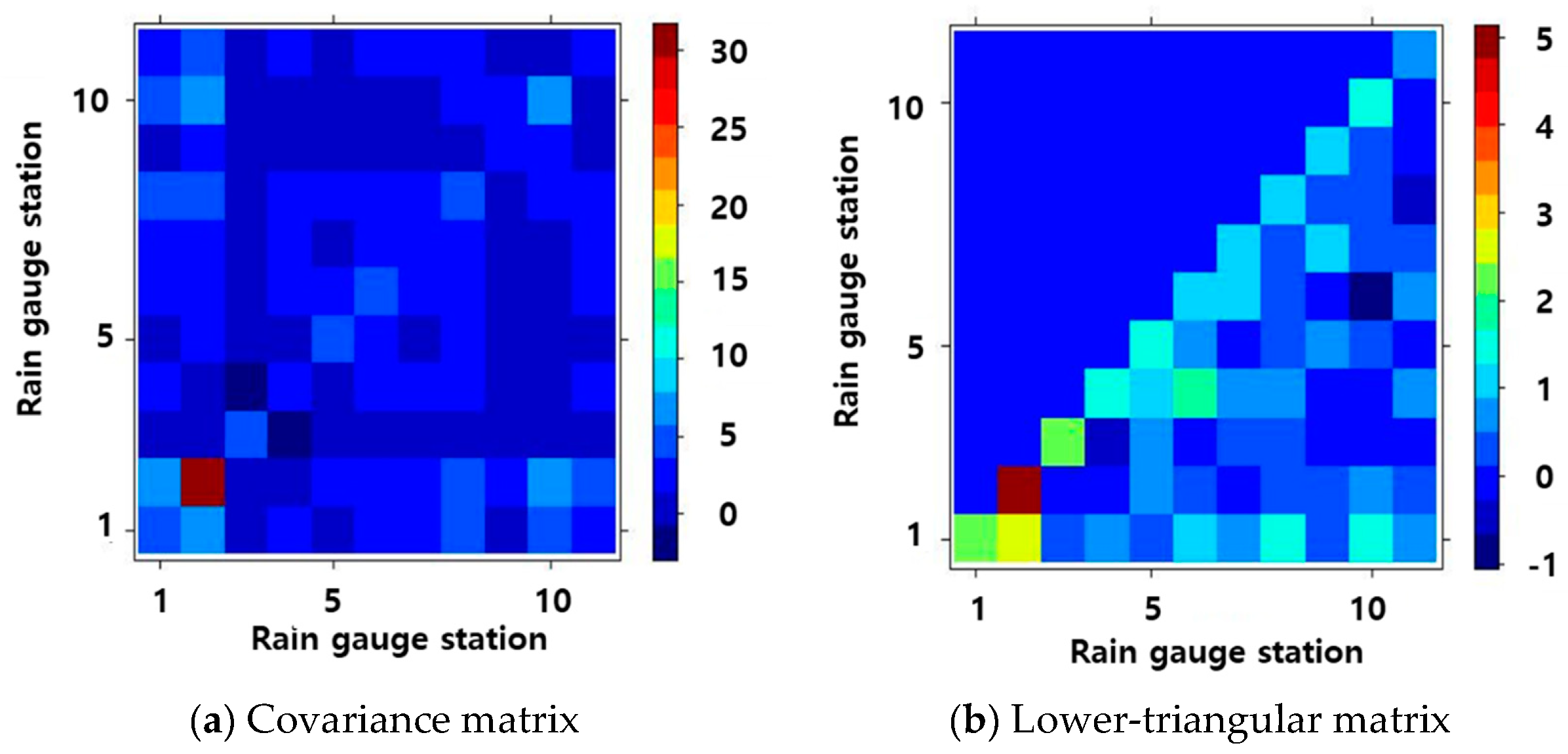
To generate a perturbation () using Equation (9), the covariance must be estimated. We obtained the covariance matrix between observation stations using Equations (4) and (5), and the results are shown in Figure 6. Figure 6a indicates the matrix generated from the estimation of the covariance among stations. Since the upper and lower sides of the diagonal line are symmetric matrices with the same value, the lower triangular matrix was produced by Cholesky decomposition, as shown in Figure 6b.
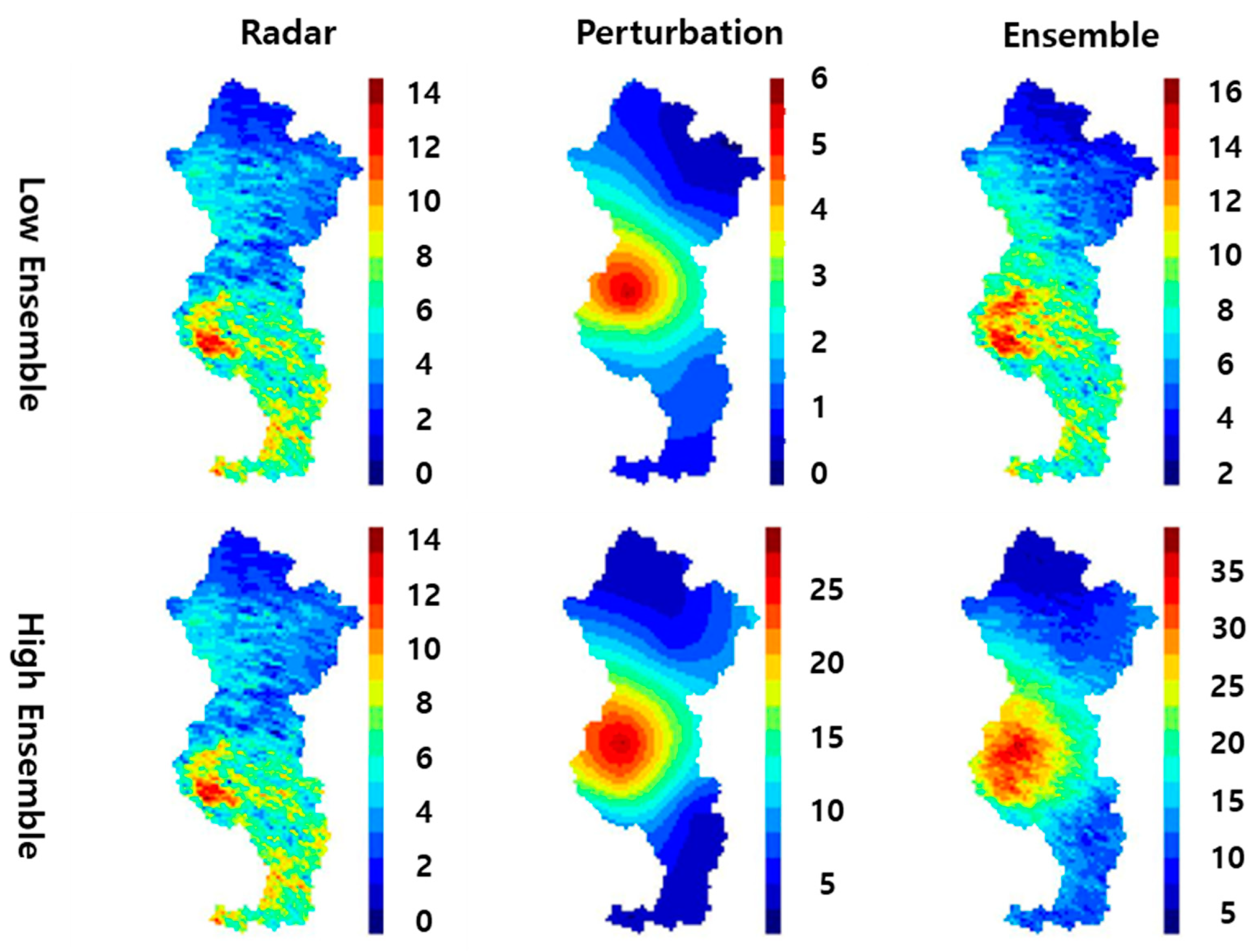
Since an ensemble is a way to express uncertainty, a sufficient number of ensembles must be generated. In this study, 100 perturbations were generated using Equation (9) to generate an ensemble that could express the uncertainty of rainfall. Figure 7 shows the maximum and minimum rainfall ensembles obtained at a chosen time. The minimum ensemble showed a maximum rainfall of 16 dBR, while the maximum ensemble showed a maximum rainfall of 35 dBR, indicating a substantial error of 19 dBR.
3.3. Runoff Analysis of Multi-Runoff Models
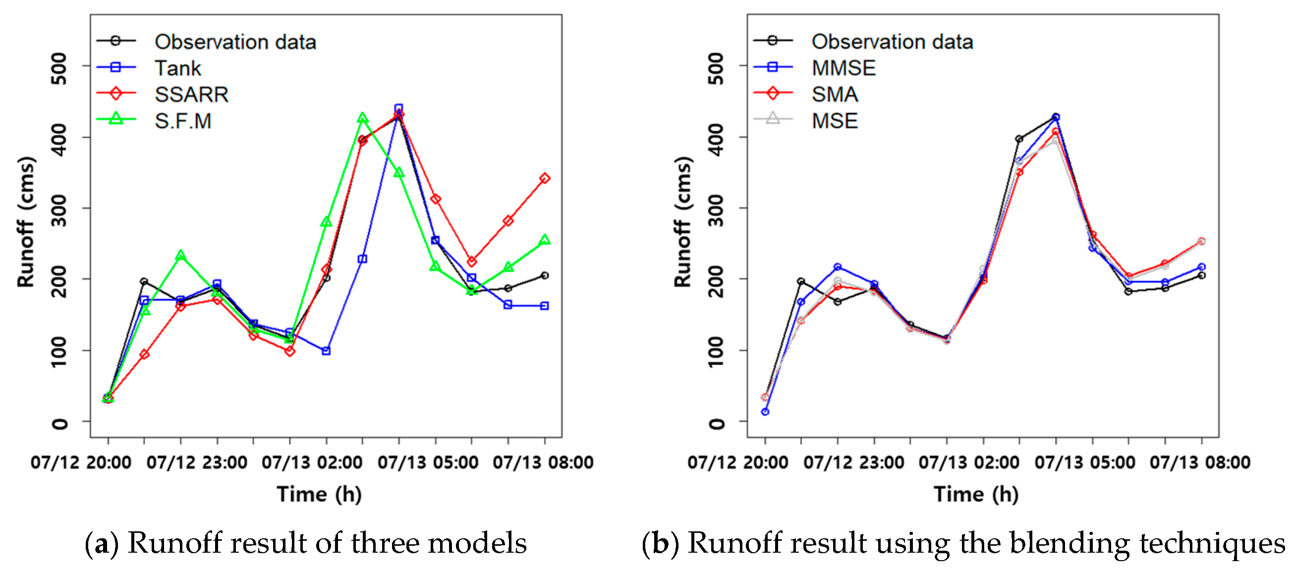
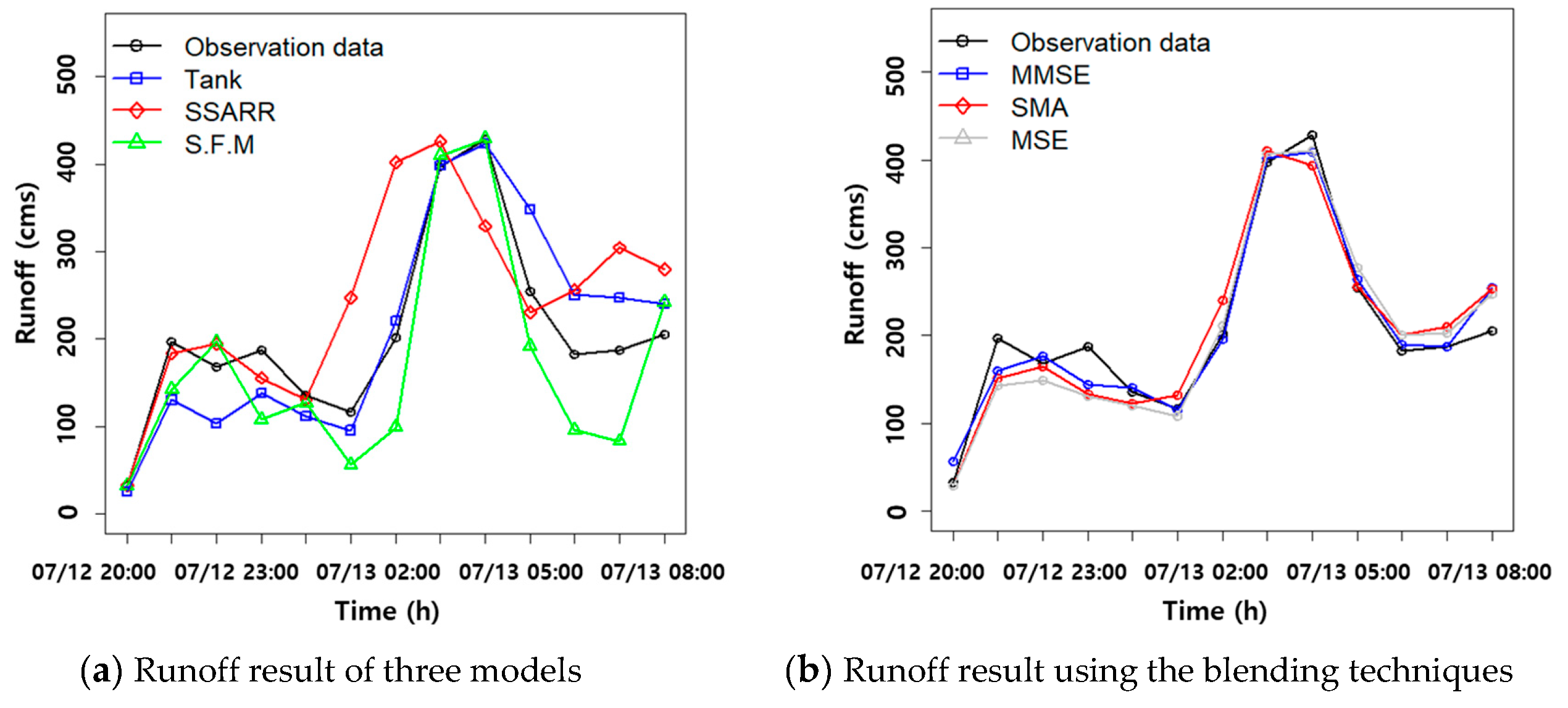
The result obtained from each model is shown in Figure 8, Figure 9 and Figure 10. Figure 8 shows the runoff result of the tank model. The observation data matched well with the radar data at the peak runoff and at the peak time. However, considering the overall runoff from the initial to the peak runoff, the simulated ground rainfall matches the observed runoff patterns best. Figure 9 shows the result of runoff of the SSARR model. From the runoff result of the radar rainfall, the peak runoff time occurs faster than the observed runoff, even if the correction is performed. This demonstrates the spatiotemporal problems of radar rainfall data. Figure 10 shows the result of runoff of the storage function model. Compared with the other models, the storage function model simulates the initial runoff with relatively high accuracy (see Table 2).
3.4. Estimation of Optimum Runoff Hydrograph Using the Blending Technique
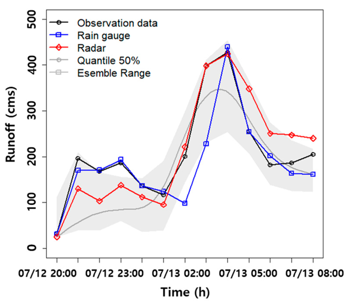
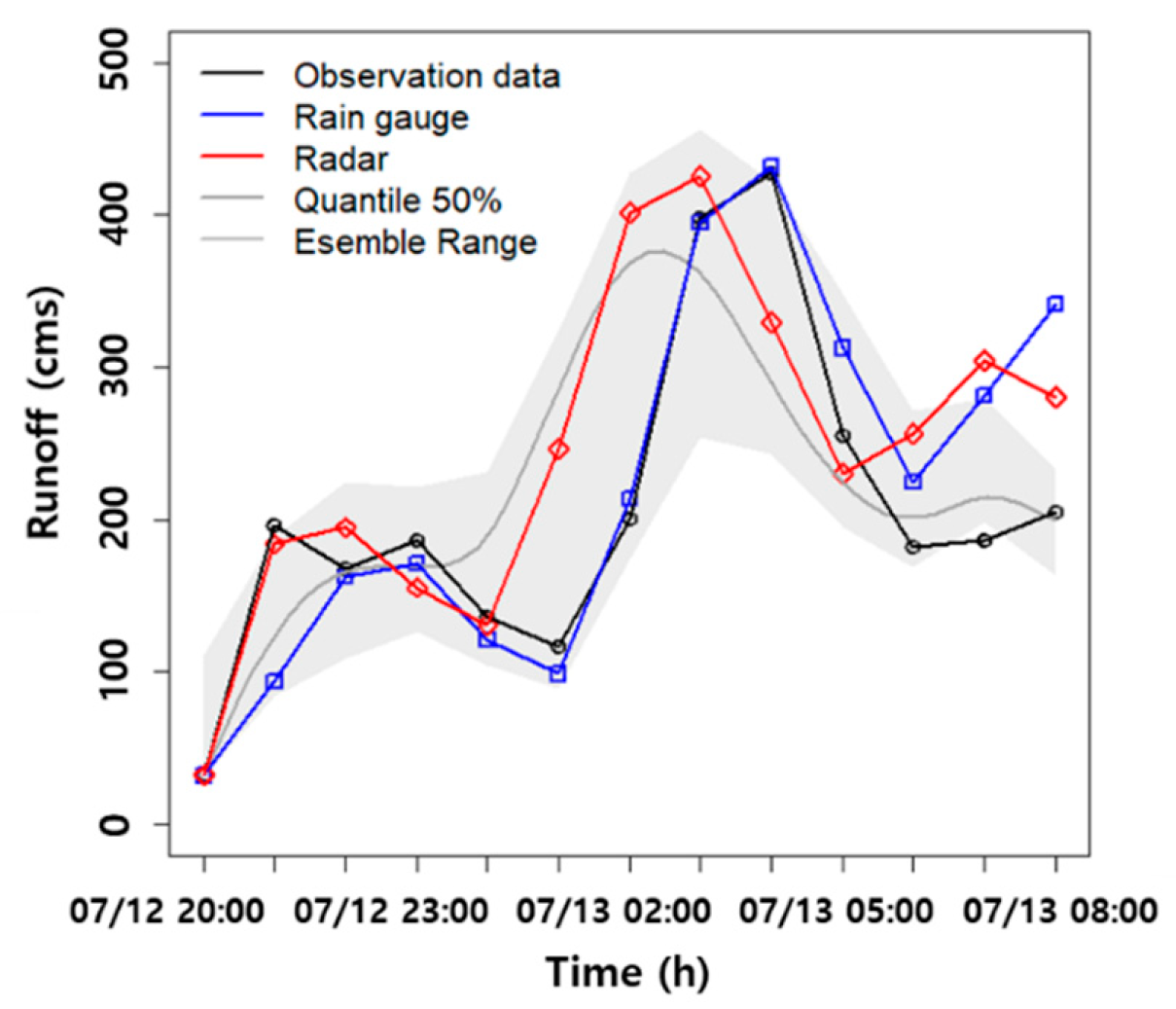
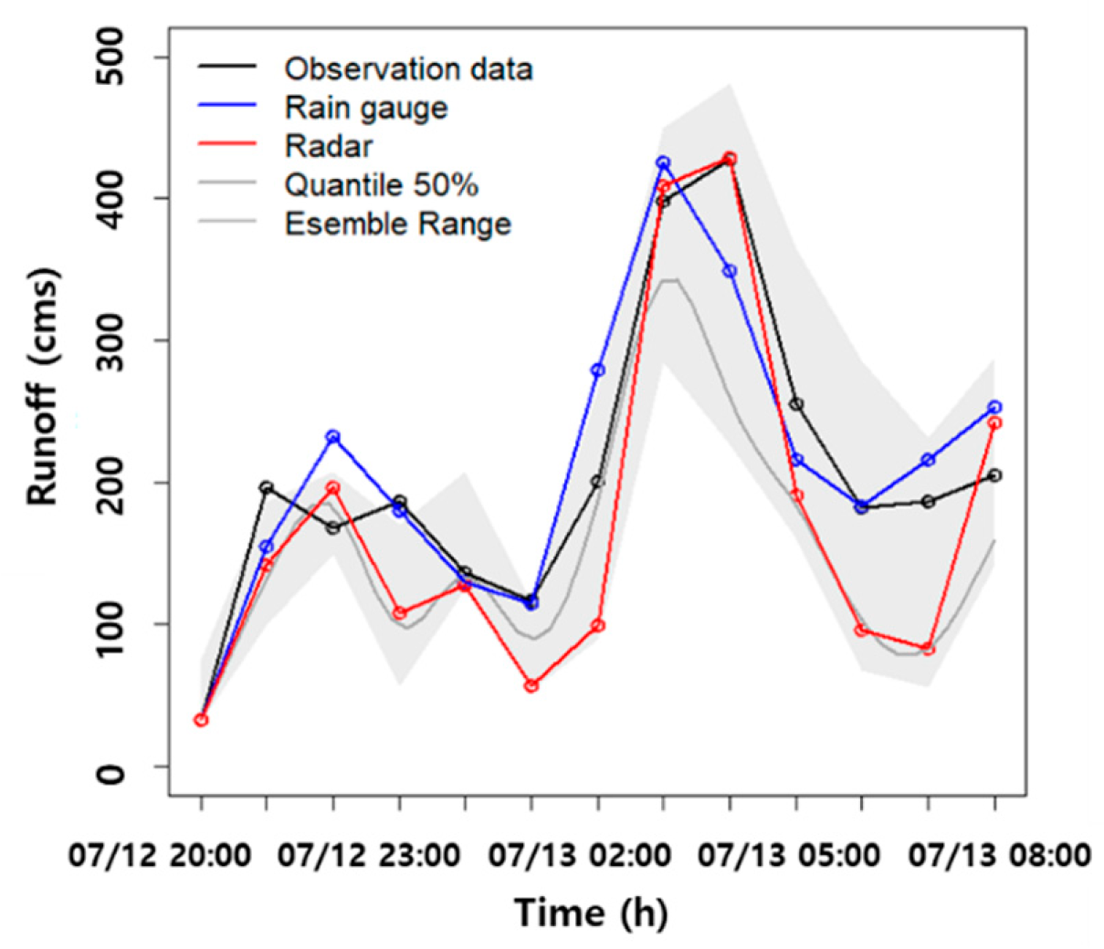
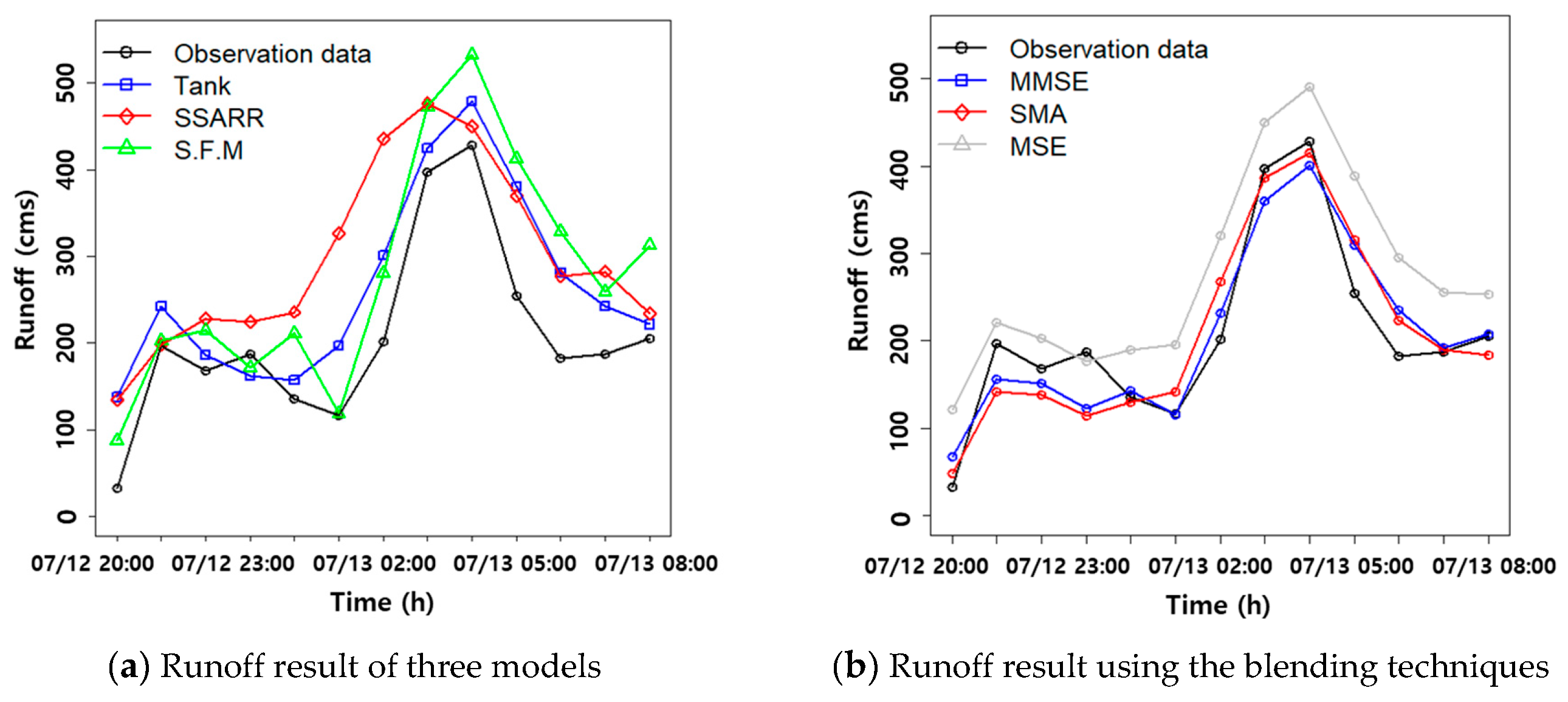
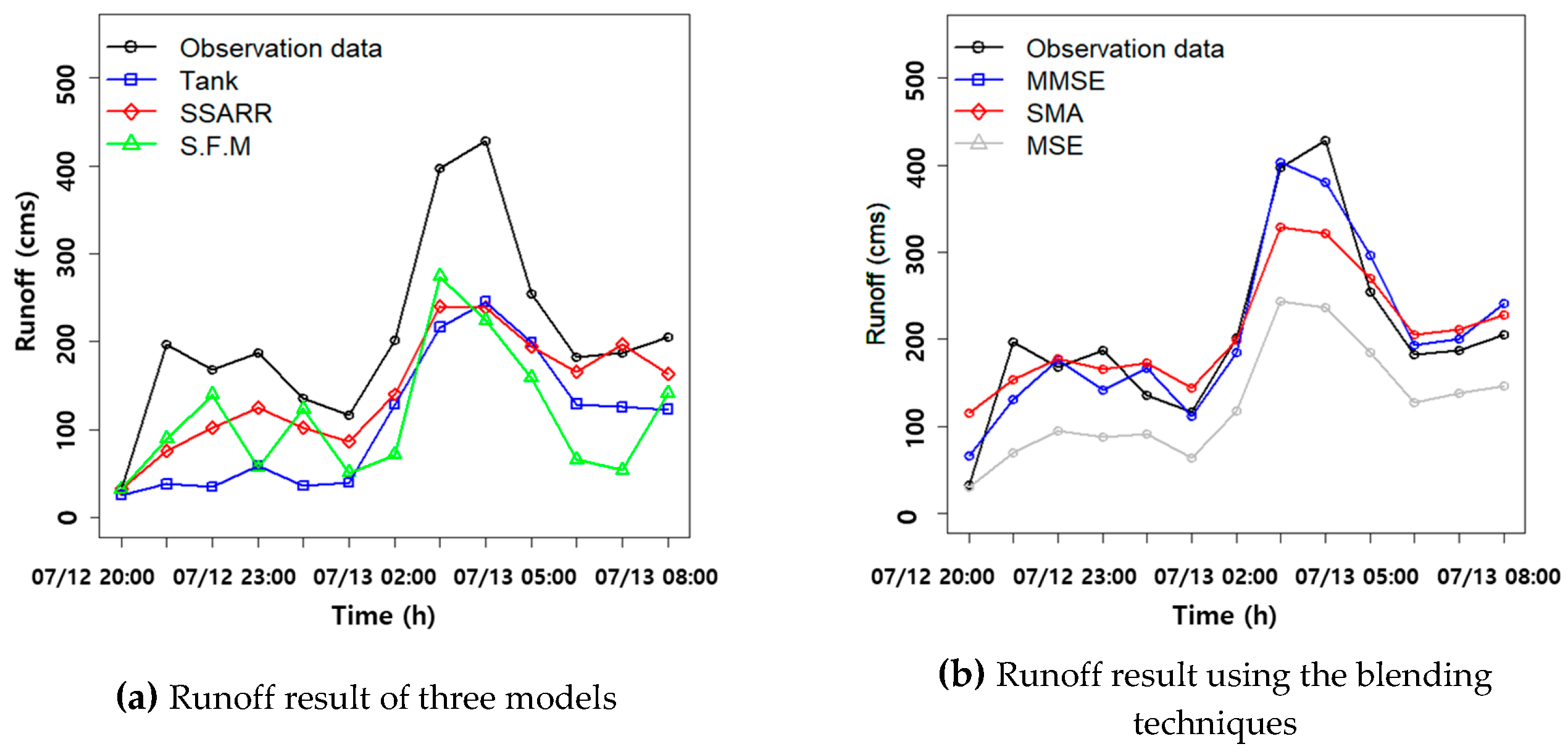
The runoff simulation results of all three models varied from model to model, even though the same rainfall data were used. Figure 11, Figure 12, Figure 13 and Figure 14 show the results with the blending techniques after integrating the runoff results of the models. Figure 11a, Figure 12a, Figure 13a and Figure 14a show the runoff results of the models using the ground rainfall, radar rainfall, the maximum ensemble, and the minimum ensemble. Figure 11b, Figure 12b, Figure 13b and Figure 14b show the runoff results in a single runoff curve, which are obtained by applying the three blending techniques, using the runoff results of the three hydrologic models as input data. The results of the blended runoff for each rainfall data reflect the observed runoff quite well.
Three blended runoff hydrographs were derived for each rainfall event. It is necessary to choose an optimal blending runoff curve that is least different to the observed runoff. To verify the efficiency of each blending runoff curve, the optimal blending runoff curve was estimated using three evaluation methods: The mean absolute error (MAE), the root mean squared error (RMSE), and the mean absolute percentage error (MAPE). The results are shown in Table 3, Table 4, Table 5 and Table 6.
Table 3 shows the evaluation index obtained by comparing the three blending techniques with the observed runoff using the ground rainfall data. The MMSE blending technique showed the best result with an error of around 5.1% and was selected as the optimum blending runoff hydrograph for the ground rainfall data. Table 4 shows the results of using the radar rainfall data. The radar rainfall also showed the best result with MMSE with an error of around 9.2%, so it was selected as the optimum blending runoff hydrograph for the radar rainfall data as well.
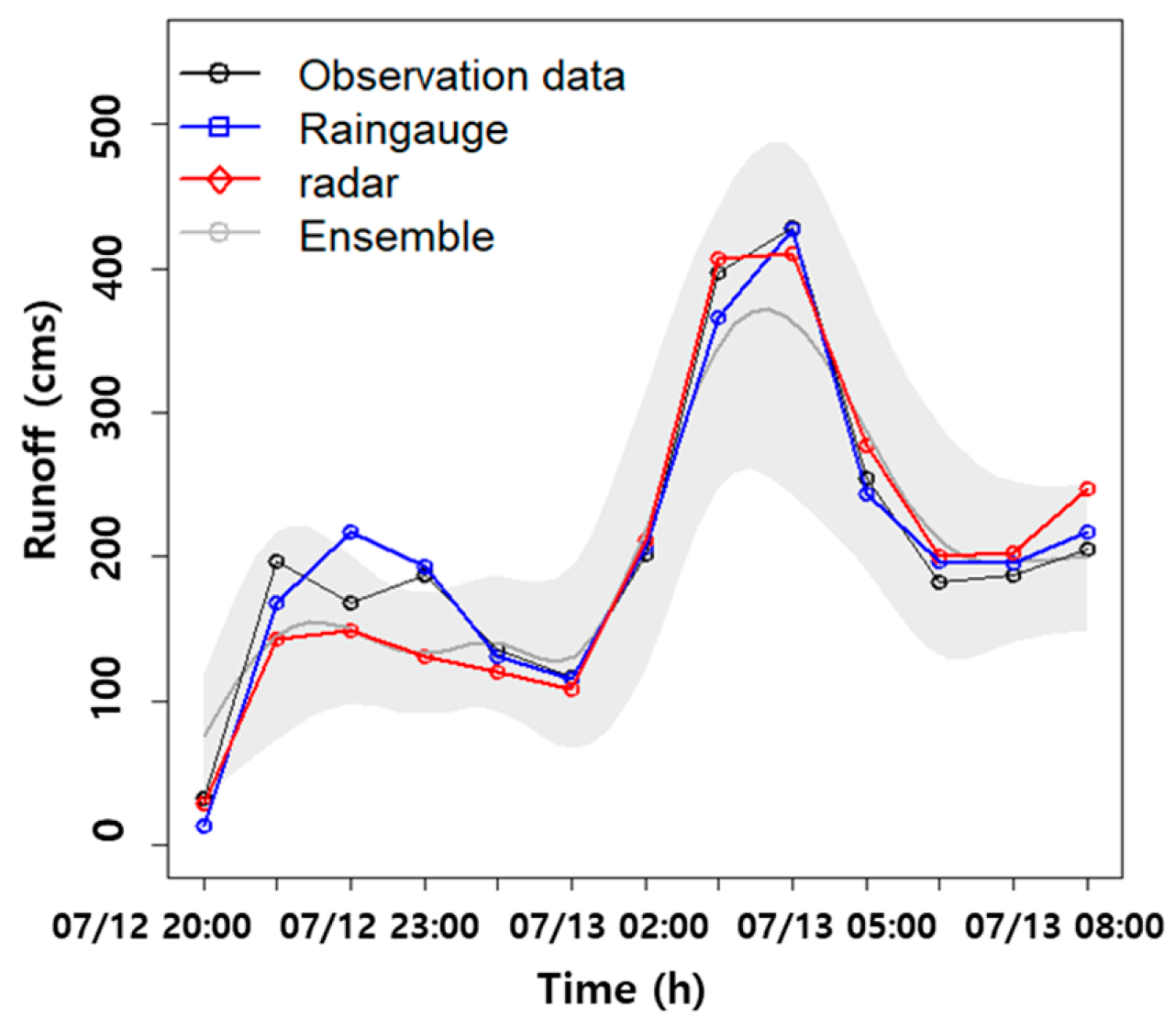
Table 5 and Table 6 show the results of using the minimum and maximum rainfall ensemble data. The ensemble rainfall data indicate the level of uncertainty of rainfall. However, the blending technique is used to reduce the uncertainty, based on the observed runoff data. When the ensemble rainfall data are applied to the blending technique, the uncertainty of the rainfall disappears. Therefore, instead of using the MMSE blending technique with the lowest error, we used the MSE blending technique with the highest error as the optimum blending runoff hydrograph for the ensemble rainfall data to express the uncertainty of ensemble rainfall. The optimal blending technique for each rainfall data is summarized in Figure 15. The runoff curves for all three rainfall data are close to the observed runoff.
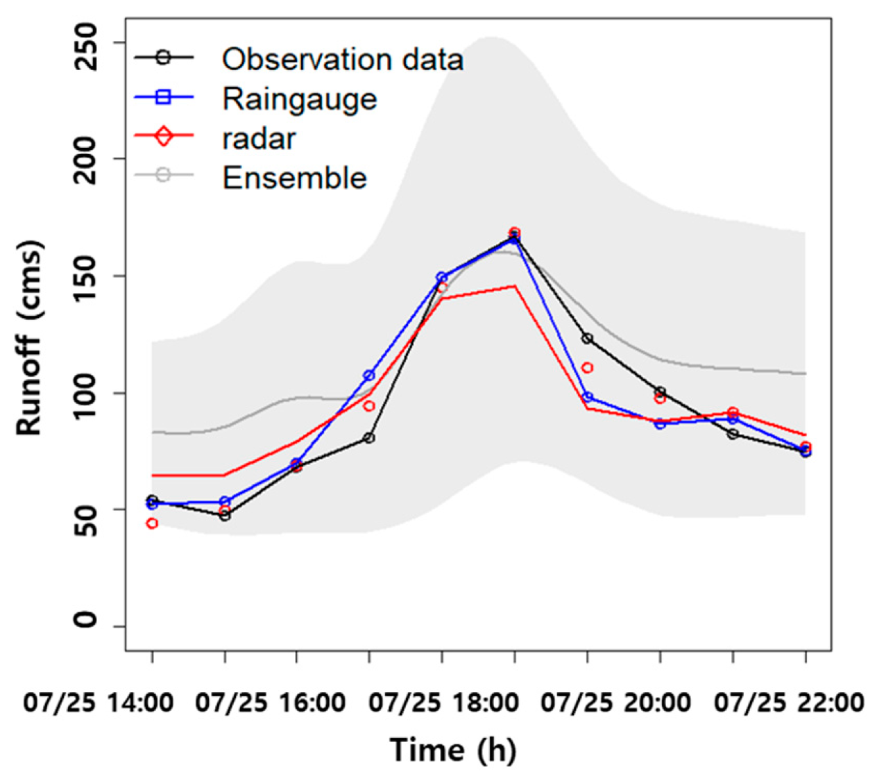
The accuracy of the rainfall ensembles and the blending techniques was evaluated by applying different rainfall events. The events from 14:00 to 23:00 on 25 July 2015 were selected for the verification, and the results are shown in Figure 16. During the verification event, the MMSE method again showed the best result with an error of 7.03–9.46%, and the MSE method showed high uncertainty of 11.31–46.93%. This confirms that the results of the hydrologic models simulated the observed runoff well when the rainfall ensembles and the blending techniques were applied.
4. Conclusions
This study generated probabilistic rainfall ensembles with error between radar and ground rainfall data to confirm the uncertainty of rainfall. Blending techniques were applied to the results of several runoff hydrologic models to determine a single runoff hydrograph. The results are summarized as follows:
- To generate rainfall ensembles, the errors of observed data and the radar data were modeled. The rainfall ensembles showed that the uncertainty of the rainfall ensemble was high when the radar was underestimated, due to topographic effects such as rainfall intensity and mountain shielding;
- A runoff analysis was performed to confirm the uncertainty of the runoff models by using station rainfall data, radar rainfall data, and ensemble rainfall data in the tank model, SSARR model, and the storage function model. Even with the same rainfall data, the runoff results of the models were all different, which confirmed the uncertainty of the runoff models;
- To reduce the uncertainty of the runoff models, three integrated runoff curves were generated by applying three blending techniques (MMSE, SMA, and MSE) to the runoff results of the three models. The results showed that the MMSE blending runoff curve showed an error of around 5.1%, compared to the observed runoff when using the station rainfall data, and around 9.2%, compared to the observed runoff using the radar rainfall data. Therefore, the MMSE blending technique was selected as the optimum runoff hydrograph;
- A verification event was used to confirm the results. The MMSE technique showed the best result with an error margin of 7.03–9.46%, while the MSE technique showed the highest uncertainty with an error margin of 11.31–46.93%.
Taking into account the results obtained in this study, the uncertainty of radar rainfall was expressed by generating a rainfall ensemble and reducing the uncertainty of the runoff model by applying the optimal blending technique. A rainfall ensemble reflecting the temporal and spatial error of rainfall can help make more efficient decisions in flood warning.
Author Contributions
This research was carried out with collaboration between all authors. H.S.K., N.K., and M.L. had the original idea for the study. H.J. and J.L. provided the research methods, and S.K. arranged the research. M.L. with N.K. conducted the research and drafted the manuscript. All authors discussed the structure of the manuscript and commented on it at all stages.
Funding
This subject is supported by the Ministry of Environment (MOE) of Korea as a “Water Management Research Program.”
Conflicts of Interest
The authors declare no conflict of interest.
References
- Kim, S.; Noh, H.; Jung, J.; Jun, H.; Kim, H.S. Assessment of the impacts of global climate change and regional water projects on streamflow characteristics in the Geum River Basin in Korea. Water 2016, 8, 91. [Google Scholar] [CrossRef]
- Kim, D.; Kim, J.; Joo, H.; Han, D.; Kim, H.S. Future water quality analysis of the Anseongcheon River basin, Korea under climate change. Membr. Water Treat. 2019, 10, 1–11. [Google Scholar]
- Chiang, Y.M.; Chang, F.J.; Jou, B.J.; Lin, P.F. Dynamic ANN for precipitation estimation and forecasting from radar observations. J. Hydrol. 2007, 334, 250–261. [Google Scholar] [CrossRef]
- Seck, I.; Van Baelen, J. Geostatistical Merging of a Single-Polarized X-Band Weather Radar and a Sparse Rain Gauge Network over an Urban Catchment. Atmosphere 2018, 9, 496. [Google Scholar] [CrossRef]
- Adirosi, E.; Roberto, N.; Montopoli, M.; Gorgucci, E.; Baldini, L. Influence of disdrometer type on weather radar algorithms from measured DSD: Application to Italian climatology. Atmosphere 2018, 9, 360. [Google Scholar] [CrossRef]
- Kuriqi, A.L. Assessment and quantification of meteorological data for implementation of weather radar in mountainous regions. Mausam 2016, 67, 789–802. [Google Scholar]
- Kang, N.-R.; Noh, H.-S.; Lee, J.-S.; Lim, S.-H.; Kim, H.-S. Runoff simulation of an urban drainage system using radar rainfall data. J. Wetl. Res. 2013, 15, 413–422. [Google Scholar] [CrossRef]
- Kim, S.; Noh, H.; Kang, N.; Lee, K.; Kim, Y.; Lim, S.; Kim, H.S. Noise reduction analysis of radar rainfall using chaotic dynamics and filtering techniques. Adv. Meteorol. 2014, 2014. [Google Scholar] [CrossRef]
- Priestley, M.B. Spectral Analysis and Time Series; Academic Press: London, UK, 1981. [Google Scholar]
- Germann, U.; Berenguer, M.; Sempere-Torres, D.; Salvade, G. Ensemble radar precipitation estimation-A new topic on the radar horizon. In Proceedings of the Fourth European Conference on Radar in Meteorology and Hydrology, Barcelona, Spain, 18–22 September 2006; pp. 18–22. [Google Scholar]
- Germann, U.; Berenguer, M.; Sempere-Torres, D.; Zappa, M. REAL-Ensemble radar precipitation estimation for hydrology in a mountainous region. Q. J. R. Meteorol. Soc. 2009, 135, 445–456. [Google Scholar] [CrossRef]
- Dai, Q.; Han, D.; Rico-Ramirez, M.A.; Islam, T. Modelling radar-rainfall estimation uncertainties using elliptical and Archimedean copulas with different marginal distributions. Hydrol. Sci. J. 2014, 59, 1992–2008. [Google Scholar] [CrossRef]
- Kang, N.-R.; Joo, H.-J.; Lee, M.-J.; Kim, H.-S. Generation of radar rainfall ensemble using probabilistic approach. J. Korea Water Resour. Assoc. 2017, 50, 155–167. [Google Scholar]
- Bates, J.M.; Granger, C.W.J. The combination of forecasts. J. Oper. Res. Soc. 1969, 20, 451–468. [Google Scholar] [CrossRef]
- Al-Safi, H.I.J.; Kazemi, H.; Sarukkalige, P.R. Comparative study of conceptual versus distributed hydrologic modelling to evaluate the impact of climate change on future runoff in unregulated catchments. J. Water Clim. Chang. 2019. [Google Scholar] [CrossRef]
- Al-Safi, H.I.J.; Sarukkalige, P.R. The application of conceptual modelling to assess the impacts of future climate change on the hydrological response of the Harvey River catchment. J. Hydro-Environ. Res. 2018. [Google Scholar] [CrossRef]
- Mcleod, I.; Noakes, D.; Hipel, K.W.; Thompstone, R.M. Combining hydrologic forecasts. J. Water Resour. Plan. Manag. 1987, 113, 29–41. [Google Scholar] [CrossRef]
- Georgakakos, K.P.; Seo, D.-J.; Gupta, H.; Schaake, J.; Butts, M.B. Towards the characterization of streamflow simulation uncertainty through multimodel ensembles. J. Hydrol. 2004, 298, 222–241. [Google Scholar] [CrossRef]
- Li, W.; Sankarasubramanian, A. Reducing hydrologic model uncertainty in monthly streamflow predictions using multimodel combination. Water Resour. Res. 2012, 48. [Google Scholar] [CrossRef]
- Ajami, N.K.; Duan, Q.; Gao, X.; Sorooshian, S. Multimodel combination techniques for analysis of hydrological simulations. J. Hydrometeorol. 2006, 7, 755–768. [Google Scholar] [CrossRef]
- Kim, J.S.; Yoon, S.K.; Moon, Y.I. Development of rating curve for high water level in an urban stream using Monte Carlo simulation. J. Korean Soc. Civ. Eng. 2013, 33, 1433–1446. [Google Scholar] [CrossRef]
- Dai, Q.; Han, D.; Zhuo, L.; Zhang, J.; Islam, T.; Srivastava, P.K. Seasonal ensemble generator for radar rainfall using copula and autoregressive model. Stoch. Environ. Res. Risk Assess. 2016, 30, 27–38. [Google Scholar] [CrossRef]
- Sugawara, M. On the analysis of runoff structures about several Japanese rivers. Jpn. J. Geophys. 1961, 2, 1–76. [Google Scholar]
- Lee, A.; Cho, S.; Kang, D.K.; Kim, S. Analysis of the effect of climate change on the Nakdong river stream flow using indicators of hydrological alteration. J. Hydro-Environ. Res. 2014, 8, 234–247. [Google Scholar] [CrossRef]
- Paik, K.-R.; Kim, J.-H.; Kim, H.-S.; Lee, D.-R. A conceptual rainfall-runoff model considering seasonal variation. Hydrol. Process. 2005, 19, 3837–3850. [Google Scholar] [CrossRef]
- Kim, J.; Kim, D.; Joo, H.; Noh, H.; Lee, J.; Kim, H.S. Case study: On objective functions for the peak flow calibration and for the representative parameter estimation of the basin. Water 2018, 10, 614. [Google Scholar] [CrossRef]
- Kimura, T. The Flood Runoff Analysis Method by the Storage Function Model; The Public Works Research Institute, Ministry of Construction: Tsukuba, Japan, 1961.
- Krishnamurti, T.N.; Kishtawal, C.M.; Zhang, Z.; LaRow, T.; Bachiochi, D.; Williford, E.; Surendran, S. Multimodel ensemble forecasts for weather and seasonal climate. J. Clim. 2000, 3, 4196–4216. [Google Scholar] [CrossRef]
- Lee, G.; Zawadzki, I. Radar calibration by gage, disdrometer, and polarimetry: Theoretical limit caused by the variability of drop size distribution and application to fast scanning operational radar data. J. Hydrol. 2006, 328, 83–97. [Google Scholar] [CrossRef]
- Kwon, S.; Lee, G.; Jung, S.H.; Park, H.S.; Suk, M.K.; Cha, J.W.; Lee, C.K. Evaluation Radar and KNU QPE Algorithm. In Proceedings of the International Weather Radar Workshop, Daegu, Korea, 1–2 November 2012. [Google Scholar]
- Lyu, G.; Jung, S.H.; Nam, K.Y.; Kwon, S.; Lee, C.R.; Lee, G. Improvement of radar rainfall estimation using radar reflectivity data from the hybrid lowest elevation angles. J. Korean Earth Sci. Soc. 2015, 36, 109–124. [Google Scholar] [CrossRef]
Figure 1.
Diagram of the study.

Figure 2.
Water level and rainfall stations in Jungrang Basin.

Figure 3.
Accumulated rainfall amount (mm/10 min) during (a) Event 1 and (b) Event 2, observed at KWK radar station, respectively.
Figure 3.
Accumulated rainfall amount (mm/10 min) during (a) Event 1 and (b) Event 2, observed at KWK radar station, respectively.

Figure 4.
Movement of rainfall: Event 2 (25 July 2015 14:00–23:00).

Figure 5.
Mean error and digital elevation models (DEM) of Jungrang Basin.

Figure 6.
Covariance matrix and lower-triangular matrix.

Figure 7.
An example of the generated ensemble rainfall—13 July 2013 06:00.

Figure 8.
Runoff hydrograph using tank model.

Figure 9.
Runoff hydrograph using SSARR.

Figure 10.
Runoff hydrograph using storage function model.

Figure 11.
Runoff hydrograph using the observation data.

Figure 12.
Runoff hydrograph using the radar data.

Figure 13.
Runoff hydrograph using the maximum rainfall ensemble.

Figure 14.
Runoff hydrograph using the minimum rainfall ensemble.

Figure 15.
Optimum runoff hydrograph using the blending technique.

Figure 16.
Optimum runoff hydrograph using the blending technique in the verification event.


Table 1.
Rainfall events and characteristics of radar data.
| Rainfall Event | 12 July 2013 20:00 to 13 July 13:00/ 25 July 2015 14:00 to 25 July 23:00 | |
| Rainfall Station | Yangju, Gwangneung, Uijeongbu, Dongdaemun, Dobong, Gangbuk, Nowon, Sungbuk, Jungrang, Sungdong, Gwangjin | |
| Radar data: KWK Radar | Latitude, longitude | 37.4439°, 126.9639° |
| Spatial resolution | 250 m | |
| Scam elevation | 0°, 0.4°, 0.8°, 1.2°, 1.6°, 2.0°, 3.0°, 4.2°, 5.7°, 7.5°, 9.8°, 12.5° | |
| Radar height | 641 m | |
| Wave length | 11 cm | |
| Beam width | 0.9° | |
Table 2.
Performance statistics of initial runoff simulation.
| Index | R2 | RMSE | |||
|---|---|---|---|---|---|
| Model | Rain Gauge | Radar | Rain Gauge | Radar | |
| Tank model | 0.86 | 0.92 | 57.57 | 48.60 | |
| SSARR model | 0.88 | 0.72 | 58.30 | 85.47 | |
| Storage function model | 0.91 | 0.92 | 42.83 | 60.67 | |
Table 3.
Evaluation of blending technique using rain gauge data.
| Blending | MMSE | SMA | MSE | |
|---|---|---|---|---|
| Index | ||||
| MAE | 9.420 | 14.874 | 12.486 | |
| RMSE | 16.279 | 20.885 | 20.243 | |
| MAPE | 0.051 | 0.084 | 0.061 | |
Table 4.
Evaluation of blending technique using radar data.
| Blending | MMSE | SMA | MSE | |
|---|---|---|---|---|
| Index | ||||
| MAE | 14.859 | 28.001 | 26.665 | |
| RMSE | 19.757 | 33.496 | 33.209 | |
| MAPE | 0.092 | 0.161 | 0.141 | |
Table 5.
Evaluation of blending technique using maximum ensemble data.
| Blending | MMSE | SMA | MSE | |
|---|---|---|---|---|
| Index | ||||
| MAE | 30.121 | 33.889 | 73.337 | |
| RMSE | 34.607 | 39.996 | 82.431 | |
| MAPE | 0.230 | 0.200 | 0.563 | |
Table 6.
Evaluation of blending technique using minimum ensemble data.
| Blending | MMSE | SMA | MSE | |
|---|---|---|---|---|
| Index | ||||
| MAE | 13.611 | 25.562 | 49.102 | |
| RMSE | 17.535 | 30.723 | 57.938 | |
| MAPE | 0.171 | 0.307 | 0.469 | |
© 2019 by the authors. Licensee MDPI, Basel, Switzerland. This article is an open access article distributed under the terms and conditions of the Creative Commons Attribution (CC BY) license (http://creativecommons.org/licenses/by/4.0/).
Share and Cite
MDPI and ACS Style
Lee, M.; Kang, N.; Joo, H.; Kim, H.S.; Kim, S.; Lee, J. Hydrological Modeling Approach Using Radar-Rainfall Ensemble and Multi-Runoff-Model Blending Technique. Water 2019, 11, 850. https://doi.org/10.3390/w11040850
AMA Style
Lee M, Kang N, Joo H, Kim HS, Kim S, Lee J. Hydrological Modeling Approach Using Radar-Rainfall Ensemble and Multi-Runoff-Model Blending Technique. Water. 2019; 11(4):850. https://doi.org/10.3390/w11040850
Chicago/Turabian StyleLee, Myungjin, Narae Kang, Hongjun Joo, Hung Soo Kim, Soojun Kim, and Jongso Lee. 2019. "Hydrological Modeling Approach Using Radar-Rainfall Ensemble and Multi-Runoff-Model Blending Technique" Water 11, no. 4: 850. https://doi.org/10.3390/w11040850
Note that from the first issue of 2016, this journal uses article numbers instead of page numbers. See further details here.