A New Uncertainty Measure for Assessing the Uncertainty Existing in Hydrological Simulation

Abstract

The absence of aggregated uncertainty measures restricts the assessment of uncertainty in hydrological simulation. In this work, a new composite uncertainty measure is developed to evaluate the complex behaviors of uncertainty existing in hydrological simulation. The composite uncertainty measure is constructed based on a framework, which includes three steps: (1) identification of behavioral measures by analyzing the pairwise correlations among different measures and removing high correlations; (2) weight assignment by means of a new hierarchical weight assembly (HWA) approach incorporating the intra-class and inter-class weights; (3) construction of a composite uncertainty measure through incorporating multiple properties of the measure matrix. The framework and the composite uncertainty measure are demonstrated by case studies in uncertainty assessment for hydrological simulation. Results indicate that the framework is efficient to generate a composite uncertainty index (denoted as CUI) and the new measure CUI is competent for uncertainty evaluation. Besides, the HWA approach performs well in weighting, which can characterize subjective and objective properties of the information matrix. The achievement of this work provides promising insights into the performance comparison of uncertainty analysis approaches, the selection of proper cut-off threshold in the GLUE method, and the guidance of reasonable uncertainty assessment in a range of environmental modelling.

1. Introduction

Uncertainty is a term used across many disciplines without identical definitions, but in essence it is related to the variable associated with the difference between the true state of a system and its observational or theoretical assessment at a specific space and time [1]. Robust simulation on streamflow is of great importance for disaster mitigation, water resources management and ecosystem maintenance, especially under the changing environment [2,3,4,5]. Uncertainties in simulated or predicted streamflow are associated with many factors, including inputs (difference between observed values and true values), model structure (unaccounted processes, empirical equations, and numerical errors), and model parameters (incomplete knowledge of parameter values, ranges, and their physical meaning) [6,7]. Uncertainties inherently exist in hydrological simulation [8], influencing the decision making on water resources management and ecosystem maintenance [9,10,11].

Uncertainty analysis is the means of calculating and representing the certainty with which the model results represent reality [12]. To estimate potential uncertainties in model outputs, several uncertainty analysis methods have been developed [13,14,15]. Some of these methods include: the generalized likelihood uncertainty estimate (GLUE) method [13], the Bayesian Markov chain Monte Carlo (MCMC) method [16], and the Bayesian model averaging (BMA) method [17]. Ajami et al. [18] proposed the integrated Bayesian uncertainty estimator (IBUNE) to account for the major uncertainties associated with model input, parameters, and structure in hydrologic prediction. Zhou et al. [19] investigated the use of an epsilon-dominance non-dominated sorted genetic algorithm II to improve the sampling efficiency for multiple metrics uncertainty analysis using GLUE.

Despite these advances in the studies of uncertainty in hydrological simulation, it should be borne in mind that the above-mentioned uncertainty assessment methods could bring additional uncertainties into the application [20]. As forms of mathematical models, they are subject to errors of uncertainties in their underlying assumptions and structure, as well as in the determination of parameters (e.g., the setting of cut-off threshold in GLUE). It follows that their uncertainty assessment indices must also reflect such uncertainties. In these uncertainty assessment methods, the output of the hydrological modelling exercise for each time step is no longer simply a single numerical value (point estimate) of discharge or stage, but rather an interval defined by the prediction bounds obtained under a certain confidence level.

The generation of quantitative measures of confidence in a model’s results is essential for providing guidance about the weight which should be given to the model in decision making, and for indicating where the model may need to be improved. According to Melching and Singh [21], confidence intervals are used to define ranges (i.e., 95%) within which the mean estimate will exist with specified probability. It means that the model outputs are commonly represented by a range of values at a certain confidence level (the called uncertainty interval). Many indices have been proposed and applied to assess the simulation accuracy of hydrological models [22]. Apart from their use in describing the properties of the prediction bounds, such indices can also serve as the criteria for comparing the prediction bounds generated from different assessment methods or schemes.

In comparing such different generated predictions bounds, their most desirable characteristics, expressed through indices, need to be identified. Some uncertainty indices or measures [23,24,25] were developed to quantitatively evaluate the uncertainty interval of hydrological simulation. A series of widely-used uncertainty measures are collected in

Table 1. Uncertainty measures widely used for describing uncertainty interval.

Properties	Name	Calculation
Coverage	Containing ratio(CR)	$CR=n_c/N$ [23]
Band-width	Average band-width (B)	$B=1/N{\displaystyle \sum _{i=1}^N(q_i^u-q_i^l)}$ [26]
	Average relative band-width (RB)	$RB=1/N{\displaystyle \sum _{i=1}^N[(q_i^u-q_i^l)/Q_i]}$ [20]
Symmetry	average asymmetry degree 1 (S)	$S=1/N{\displaystyle \sum _{i=1}^N\left|(q_i^u-Q_i)/(q_i^u-q_i^l)-0.5\right|}$ [20]
	average asymmetry degree 2 (Ts)	$Ts=1/N{{\displaystyle \sum _{i=1}^N\left[\left|{(q_i^u-Q_i)}^3+{(q_i^l-Q_i)}^3\right|/(q_i^u-q_i^l)\right]}}^{1/3}$ [20]
Deviation amplitude	Average deviation amplitude (D)	$D=1/N{\displaystyle \sum _{i=1}^N\left|(q_i^u-q_i^l)/2-Q_i\right|}$ [29]
	Average relative deviation amplitude (RD)	$RD=1/N{\displaystyle \sum _{i=1}^N\left|(q_i^u-q_i^l)/(2Q_i)-1\right|}$ [29]
Expectation	Average deviation of expectation (Dq)	$Dq=1/N{\displaystyle \sum _{i=1}^N\left|E{q}_i-Q_i\right|}$ [30]
	Average relative deviation of expectation (RDq)	$RDq=1/N{\displaystyle \sum _{i=1}^N\left|E{q}_i/Q_i-1\right|}$ [30]
	Nash-Sutcliffe Coefficient of Efficiency (NSCE)	$NSCE=1-{\displaystyle \sum _{i=1}^N{(E{q}_i-Q_i)}^2/}{\displaystyle \sum _{i=1}^N{(Q_i-\overline{Q})}^2}$ [30]

Note: n_c is the number of observations cover in the intervals; N is the number of observations; $q_i^u$ and $q_i^l$ is the upper and lower bounds of intervals at the ith time step respectively; Q_i is the observed discharge at the ith time step; Eq_i is the expectation of the output distribution at the ith time step; $\overline{Q}$ is the mean value of the observed discharge.

, which characterize various properties of uncertainty interval. For example, the containing ratio (CR) [23], referred to earlier, is defined as the ratio of the number of observed discharges enveloped by its prediction bounds to the total number of the observed discharges. A high CR for the estimated bounds or intervals is always the goal. The average band-width (B) [26] of the prediction bounds for the whole discharge series should be as narrow as possible.

Generally, an individual measure only describes part of the properties, which would fail to represent complex behaviors of uncertainty interval [27,28]. Some hydrologists therefore tried to employ a range of measures for joint analysis [20,27]. Chen et al. [27] analyzed the uncertainties of hydrological simulation in the source region of Yellow river by using four measures, including the percentages of observations that are contained in the calculated 95% confidence intervals, the average relative length, the average asymmetry degree, and the average deviation amplitude. However, conflicts amongst measures are reported. Xiong et al. [20] revealed that high containing ratio, narrow band-width and high symmetry could not be achieved simultaneously. Absence of a composite measure for describing complex properties of uncertainty interval heavily restricts quantitative evaluation of uncertainty in hydrological simulation [20].

A key point for constructing composite measures is to develop an approach to scientifically assemble different uncertainty measures [31]. The solution for the Multiple Attribute Decision Making (MADM) problems in robot selection in industrial engineering [32,33], programming in mathematics [34] and economic cybernetics in dynamic system [35], provides beneficial insights in handling the issue of assembling uncertainty measures. An MADM method is a procedure that specifies how attribute information is to be processed in order to arrive at a choice [36]. It is actually a method of assembling behavioral measures by well-assessed weights. From this point of view, the construction of composite uncertainty measures is an issue of feasible selection of contributing measures and weights assignment of the selected measures.

Weight assignment plays a key role in the construction of aggregated uncertainty measures. The contribution of each measure is hard to identify. There is actually no objective function (OF) because the ‘true value’ for the aggregated uncertainty behaviors does not exist. The current optimization algorithms hence fail to deal with the weighting problem [37,38]. Recently, a collection of weighting approaches has been widely used to solve the MADM problems [2,39,40], providing us with beneficial means to conduct the weights assignment. The weighting approaches are classified into three categories. Subjective weighting approaches determine weights mainly based on the subjective information matrix that reflect the subjective expertise (e.g., Delphi method [41], Least-Squares Method [42], Eigenvector Method [43], and Goal Programming Method [44,45]). In contrast, objective weighting methods calculate weights statistically with respect to the objective information matrix by using some matrix analysis algorithms (e.g., Standard Deviation Method [46], Entropy Method [47] and Linear Programming Method [35]).

Sometimes, the weights determined by objective methods are inconsistent with the decision maker’s subjective preferences. Contrariwise, the judgments of the decision makers occasionally depend on their knowledge or experience absolutely, and the error in weights to some extent is unavoidable [48]. Subsequently, assembled approaches incorporating advantages of a range of subjective and objective methods are recommended [39,49,50,51,52]. Actually, weights by approaches of the same class and different classes contribute differently. It should be embodied in calculation procedures. However, it has seldom been reported so far. Consequently, a new assembled weighting approach is urgently needed to consider the hierarchical ensemble of both inter-class and intra-class weights.

In this work, we strive to: (1) construct a consolidated framework to generate a new composite uncertainty measure to evaluate the uncertainty of hydrological simulation; (2) develop an integrated weighting approach based on a hierarchical ensemble of multiple matrix properties incorporating the intra-class and inter-class weights; and (3) develop a composite uncertainty index (CUI) by incorporating a range of uncertainty measures and well-assessed weights. The CUI is employed to assess the uncertainty interval of simulated streamflow. This study provides a new approach to evaluate the uncertainty inherently existing in hydrological simulation.

2. Methodology

2.1. The Framework for Generating A Composite Uncertainty Measure

A framework for generating a composite uncertainty measure is developed and shown in Figure 1, which includes three parts: measure identification, weight assignment, and index construction.

In the first part (measure identification), contributing measures are identified through analyzing the pairwise linear correlations among different measures, highly correlated measures are excluded [36]. Behavioral measures should not be linearly correlated strongly to avoid information overlap, whereas strong negative correlations are acceptable. Selected measures are arranged and normalized into an objective information matrix. The correlative importance for each two measures assessed based on expertise is used to construct the subjective information matrix.

A simple approach for identifying the behavioral measures is developed according to the correlation coefficient (R) matrix, which includes four steps:

Step 1: Pre-define a correlation coefficient RT as the maximum R and a number N as the limiting number of selected measures;

Step 2: Count the number of correlation coefficients larger than RT by columns in the correlation coefficient matrix;

Step 3: Re-construct the correlation coefficient matrix by deleting the row and column corresponding to the measure with the largest number of R larger than RT. If multiple measures have the same largest number, follow the principle that remain measures of different property types, andif not possible, follow the order “expectation > band-width > coverage > deviation amplitude > symmetry”.

Step 4: If the number of measures equals to N, stop, and the remaining measures are the contributing measures; otherwise, go to Step 2.

In the second part (weight assignment), weights are assigned to corresponding measures properly. It is the most important part in the framework, which is conducted by a series of classical weighting algorithms emphasizing subjective or objective information [31,48]. To overcome the insufficiency of a single weighting approach, a hierarchical weight assembly (HWA) method was developed in this work and compared with classical weighting algorithms.

In the third part (index construction), behavioral measures are synthesized with corresponding weights to build a composite uncertainty index (CUI):

$$CUI=w_1\times I_1+w_2\times I_2+\cdots +w_m\times I_m\hspace{1em}i=1,2,\dots ,m$$

(1)

where $I_i$ is the value of selected measures and $w_i$ is the corresponding weight; m denotes the number of behavioral measures. CUI ranges from 0 to 1. Larger CUI implies better performance of the uncertainty interval for hydrological simulation. Values of the measures in the CUI formula are the normalized values rather than the original ones.

It should be noted that inputs of the framework are uncertainty analysis results, namely the uncertainty interval of hydrological simulation. This paper just focuses on the uncertainty induced by model parameters.

2.2. Weight Assignment Approach

2.2.1. Subjective Weighting

Subjective weighting is to assign weights according to the relative importance amongst measures assessed by experts. Table 2 shows two assessing rules for relative importance, including the Analytic Hierarchy Process (AHP) rules [52] and the G1 rules [53,54,55]. AHP is a multi-attribute decision-making method that can reflect a priori information about the relative importance of inputs, outputs or even decision making units in the performance assessment [52]. G1 is a subjective weighting method that has the advantage of easy calculation and does not need to test the consistency of the judgment matrix [54].

Two approaches, including the weighted least square (WLS) [56,57] method and the G1 [53,54,55] approach, are commonly employed to establish the weights. WLS is based on the subjective information matrix constructed according to the AHP rules [56]. Relative importance $d_{ij}$ of the ith measure against the jth measure ($i,j=1,2,\cdots ,m$) is therefore assessed according to the rules. Store $d_{ij}$ into a matrix $D={[d_{ij}]}_{m\times m}$, which is exactly the “subjective information matrix”, satisfying: $d_{i,j}>0, d_{i,j}=1/d_{j,i}$, and $d_{i,i}=1$ for $i,j=1, 2, \cdots ,m$. G1 assigns weights without using a subjective information matrix, for details about G1 refer to Zheng [54] and Xie [55].

The weighted least square method for subjective weighting (denoted as WLSS) [56,57] is employed for subjective weighting in this work. It obtains the weight through optimizing a matrix F related to D, and the final weight is:

$$w^{\ast }=F^{-1}e/e^T{F}^{-1}e$$

(2)

where $e={(1, 1, \dots ,1)}^T$, F is a positively defined matrix in the occasion when there is at least one $d_{ij}\ne d_{ik}{d}_{kj}$ for $\forall i,j,k;i,j,k\in \{1,2,\cdots ,m\}$. Further details of the WLSS method are presented in Appendix A.

2.2.2. Objective Weighting

The uncertainty measures listed in Table 1 can form a column vector $S_i={(a_{i1}, a_{i2}, \dots ,a_{im})}^T$. Vector $S_i$ is called an “event” and the element $a_{ij}$ denotes the jth measure in the ith event ($i=1, 2, \dots , n;\hspace{1em}j=1, 2, \dots ,m$). Consisting of n possible event vectors, the $n\times m$ matrix $A=(S_1^T, S_2^T, \dots , S_n^T)$ or $A={[a_{ij}]}_{n\times m}$ named as “decision matrix” is constructed (

Table 3. Basic form of measure matrix labeled by event and measure.

Condition	Measure 1	Measure 2	……	Measure n
Event 1
∶
Event n

). Each column of the matrix corresponds to an uncertainty measure. The assembly of both uncertainty measures and events constitutes a two-dimensional decision matrix. The synthetization of multiple events and measures may greatly complicate the decision matrix into multiple dimensions with much larger matrix size.

Some uncertainty measures contribute positively to the uncertainty behaviors while others contribute negatively. For example, a large value of CR (Table 1) contributes positively to good performance, whereas a large value of B (Table 1) contributes negatively. It is the essential reason for conflicts amongst measures. To deal with the scaling and conflicting problems amongst measures, decision matrix A is handled with the following normalization [57,58]. After normalization, the measures have the same scale of 0 to 1.

For positive measures:

$$b_{ij}=\frac{a_{ij}-a_j^{\min }}{a_j^{\max }-a_j^{\min }}\hspace{1em}\hspace{1em}i=1, 2, \dots ,n; j=1, 2, \dots , m$$

(3)

for negative measures:

$$b_{ij}=\frac{a_j^{\max }-a_{ij}}{a_j^{\max }-a_j^{\min }}\hspace{1em}\hspace{1em}i=1, 2, \dots , n; j=1, 2 ,\dots , m$$

(4)

$a_j^{\max }$ and $a_j^{\min }$ are represented as follows

$$a_j^{\max }=\max (a_{1j}, a_{2j}, \dots , a_{nj})$$

(5)

$$a_j^{\min }=\min (a_{1j}, a_{2j}, \dots , a_{nj})$$

(6)

• Objective weighting method:

Five approaches, including the weighted least square method for objective weighting (WLSO) [57], standard deviation (SD) [59] method, VaRiance (VR) [59] method, Entropy method (EM) [60], and criteria importance through inter-criteria correlation (CRITIC) [59,61] method, are employed to establish the weights.

Weights by WLSO [57] can be calculated using the equation below:

$$w^{\ast }=H^{-1}e/e^T{H}^{-1}e$$

(7)

where $e={(1, 1, \dots ,1)}^T$, H is a $m\times m$ diagonal matrix.

Weights by the SD method [59] can be calculated through the formula below:

$$w_j={\sigma }_j/{\displaystyle \sum _{k=1}^m{\sigma }_k}\hspace{1em}\hspace{1em}j=1, 2, \dots , m$$

(8)

where ${\sigma }_j$ is the standard deviation of the corresponding column vector within matrix B.

Weights by VaRiance (VR) method [59] can be obtained through the formula below:

$$w_j={\sigma }_j^2/{\displaystyle \sum _{k=1}^m{\sigma }_k^2}\hspace{1em}\hspace{1em}j=1, 2, \dots , m$$

(9)

where ${\sigma }_j^2$ is the variance of the corresponding column vector within matrix B.

Entropy method (EM) [58,60] determines weights according to the equation below:

$$w_j=d_j/{\displaystyle \sum _{k=1}^m{d}_k}\hspace{1em}\hspace{1em}j=1, 2, \dots , m$$

(10)

where $d_j$ is the coefficient of the jth measure.

Weights by CRITIC method [59,61] can be obtained through the formula below:

$$w_j{=\mathrm{Z}}_j/{\displaystyle \sum _{k=1}^m{Z}_k}\hspace{1em}\hspace{1em}j=1, 2, \dots , m$$

(11)

where ${\mathrm{Z}}_j$ is a quantified label.

Further details of the methods about WLSO, SD, VR, EM, and CRITIC are shown in Appendix A.

2.2.3. Hierarchical Weight Assembly (HWA) Method

SD and VR methods are concerned with the secondary moment of measures. EM method pays attention to the chaos degree of information, while the CRITIC method focuses on the combination of both the contrast intensity and the correlations amongst different measures. These approaches have different advantages and disadvantages, it is therefore essential to build an “optimized” method with consideration of their merits. A hierarchical weight assembly (HWA) method incorporating multiple matrix properties and various approaches for uncertainty assessment is presented (Figure 1).

The HWA approach attempts to statistically incorporate multiple properties of the information matrix by an assembly of various weighting methods. Integration of the same approaches (e.g., subjective + subjective) is significantly distinct with that of different ones (e.g., subjective + objective). The subjective information matrix contains the knowledge of experts, while objective information matrix directly records the statistical properties of the simulated uncertainty interval. The information therefore ought to be treated differently. Hence, the assembly of intra-class approaches and inter-class approaches is implemented hierarchically. The hierarchical assembly is done following two steps:

(1) Intra-class Assembly

Intra-class assembly is a procedure of compositing weight sets calculated by different intra-class (subjective or objective) approaches into integrated intra-class weights. The intra-class assembly for objective weights is calculated as:

$$P{W}_{Oj}=({\displaystyle \prod _{i=1}^k{w}_{Oij}{)}^{1/k}}\hspace{1em}\hspace{1em}j=1, 2, \dots , m$$

(12)

$$w_{Oj}=P{W}_{Oj}/{\displaystyle \sum _{i=1}^{m}P{W}_{Oi}}\hspace{1em}\hspace{1em}j=1, 2, \dots , m$$

(13)

where, $w_{Oj}$ is the intra-class integrated objective weight of the jth measure, $w_{Oij}$ denotes the weight of the jth measure calculated by the ith objective weighting method, k represents the number of objective methods involved in HWA approach, and $P{W}_{Oj}$ is a variable used for storing the process weight of the jth measure. Similarly, the intra-class integration for subjective weights is calculated as:

$$P{W}_{Sj}=({\displaystyle \prod _{i=1}^t{w}_{Sij}{)}^{1/t}}\hspace{1em}\hspace{1em}j=1, 2, \dots , m$$

(14)

$$w_{Sj}=P{W}_{Sj}/{\displaystyle \sum _{i=1}^{m}P{W}_{Si}}\hspace{1em}\hspace{1em}j=1, 2, \dots , m$$

(15)

the denotation of variables can be referred to above.

(2) Inter-class Assembly

Inter-class assembly is conducted by means of linear weighted summation method [62]:

$$w_i=\phi \times w_{Oi}+\varphi \times w_{Si}\hspace{1em}\hspace{1em}i=1, 2, \dots , m$$

(16)

where $w_i$ denotes the integrated inter-class weight for the ith measure and is also the final weight of the HWA approach; $\phi$ and $\varphi$ are the two classifying coefficients. Classifying coefficients are commonly determined according to expertise. Nonetheless, we try to determine their values in a more statistical way with the help of difference coefficient $T_s$:

$$\phi =\frac{m}{m-1}{T}_s$$

(17)

$$\varphi =1-\phi$$

(18)

$$T_s=2(P_1+2P_2+\dots +m{P}_m)/m-(m+1)/m$$

(19)

where $P_1, P_2, \dots , P_m$ are the ascending sequence of the integrated intra-class subjective weights.

2.3. Uncertainty Analysis for Hydrological Modelling

In this work, the Xinanjiang model [63] (simplified as XAJ) is employed to simulate the streamflow of a catchment located in a semi-humid region of China. The uncertainty intervals of hydrological simulation are generated by means of three widely used uncertainty analysis approaches, which are introduced below (Section 2.3.2).

2.3.1. Study Basin and Data

Lushi basin (4623 km²) is a sub-basin of the Sanhuajian region located within the Yellow river basin, which is controlled by Lushi hydrological station (Figure 2). The elevation of Lushi basin ranges from 500 m and 2000 m a.s.l. A typical monsoon climate, characterized by abundant rainfall (55%–65% of the total precipitation) in rainy seasons (from July to September), dominates this mountainous area [64]. The annual mean precipitation is approximately 720 mm and the annual mean water surface evaporation is 966mm. Lack of large water control projects is one of the most attracting factors for us to choose this region. Daily data of 6 years (1982–1987) including daily precipitation, potential evapotranspiration and streamflow is collected. Data of the first year acts as the warm-up period to weaken the impacts induced by initial state variables.

2.3.2. Hydrological Model and Uncertainty Analysis Method

• Hydrological Model

XAJ model is constituted by four distinctive modules, namely three-layer evapotranspiration module, saturation excess runoff module, water source partition module, and discharge routing module. The model has been operationally applied to simulate and forecast streamflow in almost all humid and semi-humid regions of China [65]. Domains and interpretations of the 16 parameters in the XAJ model are presented in

Table 4. Parameters of the XAJ model along with their descriptions and domains.

Parameter	Description	Domains
KC	Ratio of potential evapotranspiration to pan evaporation	0.5–0.9
UM	Upper tension moisture capacity	10–20
LM	Lower tension moisture capacity	60–90
C	Coefficient of deep evapotranspiration	0.1–0.2
WM	Average soil moisture storage capacity	120–200
B	Exponent of the soil moisture storage capacity curve	0.1–0.4
IM	Ratio of the impervious to the total area of the basin	0.01–0.04
SM	Average free water storage capacity	0–50
EX	Exponent of the free water storage capacity curve	1.0–1.5
KG	Outflow coefficient of the free water storage to interflow	0.5–0.7
KI	Outflow coefficient of the free water storage to groundwater	KI + KG = 0.8
CS	Recession constant of the surface water	0.5–0.999
CI	Recession constant of the lower interflow storage	0.5–0.999
CG	Recession constant of the groundwater storage	0.5–0.999
KE	Parameter of Muskingum routing	0–40
XE	Parameter of Muskingum routing	0–0.5

. The parameters are sampled within the corresponding domains. With respect to the related parameter KI and KG, KI was sampled and KG was assigned values based on the function KI + KG = 0.8 (i.e., KG = 0.8 − KI). For more details of the model, refer to Zhao [63].

• Uncertainty Analysis Approaches

The widely used generalized likelihood uncertainty estimate (GLUE) method [66,67,68] and shuffled complex evolution metropolis algorithm (SCEM-UA) [69] are employed in our work. Considering that the SCEM-UA method with a standard likelihood measure usually generates too small an interval to cover observed points [26], we adopt the same handlings as Blasone [26], where the likelihood measure of the SCEM-UA method is changed to the Nash-Sutcliffe Coefficient of Efficiency (NSCE):

$$NSCE=1-\frac{{\displaystyle \sum _{i=1}^n{(Ob{s}_i-Si{m}_i)}^2}}{{\displaystyle \sum _{i=1}^n{(Ob{s}_i-\overline{Obs})}^2}}$$

(20)

where, $Ob{s}_i$ and $Si{m}_i$ are respectively the observation and simulation at ith time step, $\overline{Obs}$ is the mean of observations; n is the length of discharge series. In this sense, the SCEM-UA method does no longer adhere to classical statistics and can be referred to as a pseudo-Bayesian (shorten as PSCEM-UA) approach. The standard SCEM-UA (denoted as SSCEM-UA) method is employed for comparison with GLUE and PSCEM-UA methods. For more details of the GLUE and SCEM-UA methods, refer to Vrugt et al. [69].

Before conducting uncertainty assessment, setting of uncertainty analysis should be interpreted clearly. All three uncertainty analysis approaches (GLUE, PSCEM-UA and SSCEM-UA) generate parameter samples for five parallel sequences, each sequence for 10,000 samples. First 2000 of the 10,000 samples in each sequence are used for the burn-in period and abandoned. For GLUE and PSCEM-UA, cut-off thresholds should be pre-set to classify model runs into ‘behavioral’ and ‘non-behavioral’ classes. Samples with likelihoods (NSCEs) less than a pre-defined cut-off threshold are non-behavioral. The model outputs corresponding to the behavioral samples constitute the simulated values with confidence interval. For SSCEM-UA, it is conducted without using a cut-off threshold. The uncertainty measures listed in Table 1 are therefore computed according to the uncertainty interval.

3. Results

This section lists results including two parts. The first part shows the conventional uncertainty analysis. It is implemented by using a range of single uncertainty measures. The second part shows the application of the new framework to two case studies with increasing complexity. It involves the operations of each step of the framework, the demonstration for rationality of the framework, and the result analysis.

3.1. Conventional Uncertainty Assessment in The Study Region

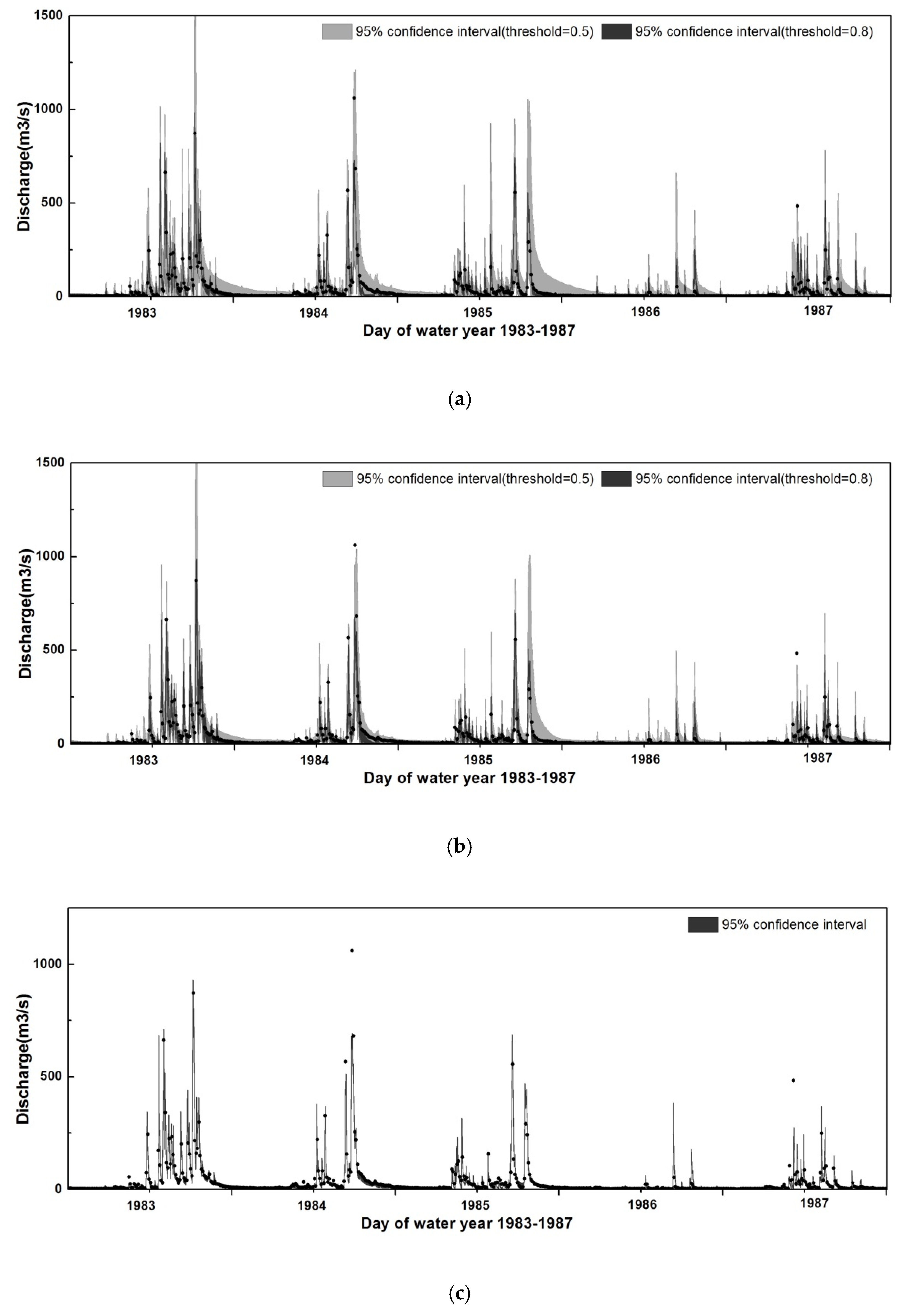
The simulated streamflow of Lushi basin by XAJ model is shown in Figure 3. The 95% confidence intervals generated by uncertainty analysis approaches at different cut-off thresholds are plotted in the figures. It is seen that the uncertainty intervals by GLUE and PSCEM-UA methods narrow sharply with the increase of thresholds from 0.5 to 0.8. As for the SSCEM-UA method, the intervals are much thinner than that of GLUE and PSCEM-UA, leading to the least coverage ratio (CR) and band width (B and RB) (

Table 5. The values of uncertainty measures generated by GLUE, PSCEM-UA and SSCEM-UA at different thresholds (shorten as Th).

Methods	Th	CR	B	RB	S	Ts	D	RD	Dq	RDq	NSCE
GLUE	0.7	0.75	46.70	2.43	0.74	0.92	16.04	0.83	16.26	0.85	0.81
	0.5	0.88	59.54	3.03	0.69	0.80	17.02	0.91	16.09	0.77	0.78
	0.1	0.90	73.18	3.76	0.69	0.77	20.09	1.16	16.45	0.74	0.77
PSCEM-UA	0.7	0.47	37.43	1.53	0.89	3.39	16.64	0.86	18.01	0.87	0.80
	0.5	0.61	45.98	2.01	0.81	1.39	16.89	0.84	18.04	0.87	0.79
	0.1	0.61	48.01	2.04	0.83	1.41	17.37	0.86	18.05	0.87	0.79
SSCEM-UA	-	0.29	7.09	0.65	1.98	2.41	12.95	0.67	12.88	0.66	0.87

). Generally, it is found that a smaller interval width always goes with less coverage ratio.

Table 5 shows the values of uncertainty measures generated by GLUE, PSCEM-UA and SSCEM-UA approaches. GLUE and PSCEM-UA are conducted at different cut-off thresholds (0.7, 0.5 and 0.1), whereas the SSCEM-UA does not need to set a cut-off threshold. A larger threshold generally implies less coverage for observed points (CR), larger asymmetry (S and Ts), but narrower band-width (B and RB) and higher NSCE. PSUEM-UA approach is robust in generating thin bands (B and RB) and a small deviation amplitude (D and RD) but powerless in generating a coverage ratio (CR) compared with GLUE. Compared with GLUE and PSUEM-UA, results of the SSUEM-UA approach are different in terms of the fact that it generates the smallest coverage (CR) and least band-width (B and RB).

3.2. Application of The Framework in Case Studies

Two cases with increasing matrix complexity in terms of dimensions and sizes are studied. Case 1: This case aims to identify a feasible threshold value in the GLUE approach. The framework is conducted in detail by three steps including measure identification, weight assignment and index construction. Case 2: This case aims to evaluate the performance of uncertainty analysis approaches. The complexity further increases with increased measure number and different confidence levels.

3.2.1. Identify Feasible Threshold Value in GLUE Approach (Case 1)

Figure 3 and Table 5 clearly show that the cut-off threshold influences the features of uncertainty intervals. The cut-off threshold is not treated as a parameter participating in the procedure of uncertainty assessment but an algorithmic parameter of the GLUE approach which needs to be pre-set before uncertainty assessment. Actually, algorithmic parameters of this kind extensively exist in a range of statistical or environmental models. How to identify the feasible values of these algorithmic parameters has not been addressed so far, motivating us to conduct this case study.

• Measure Identification

All uncertainty measures describing the uncertainty intervals generated by GLUE approach at different cut-off thresholds are computed. Measures CR and NSCE are regarded as positive measures and the remaining as negative measures. Store these measures into a decision matrix and normalize the matrix according to Equations (3) and (4). The original correlation coefficient matrix is presented in Table 6a, which is used to select behavioral or contributing measures for constructing the composite index CUI.

Five behavioral measures (CR, RB, D, Dq and RDq) are finally picked out based on a pre-defined RT = 0.8 using the method described in Section 2.1. The final correlation coefficient matrix (Table 6b) shows that these selected measures are not highly correlated in terms of the fact that the correlation coefficients are lower than RT. Actually, the majority (80%) of the correlation coefficients are smaller than 0.6. The normalized matrix of behavioral measures (objective information matrix) at different cut-off thresholds is presented in Table 6c.

• Weight Assignment

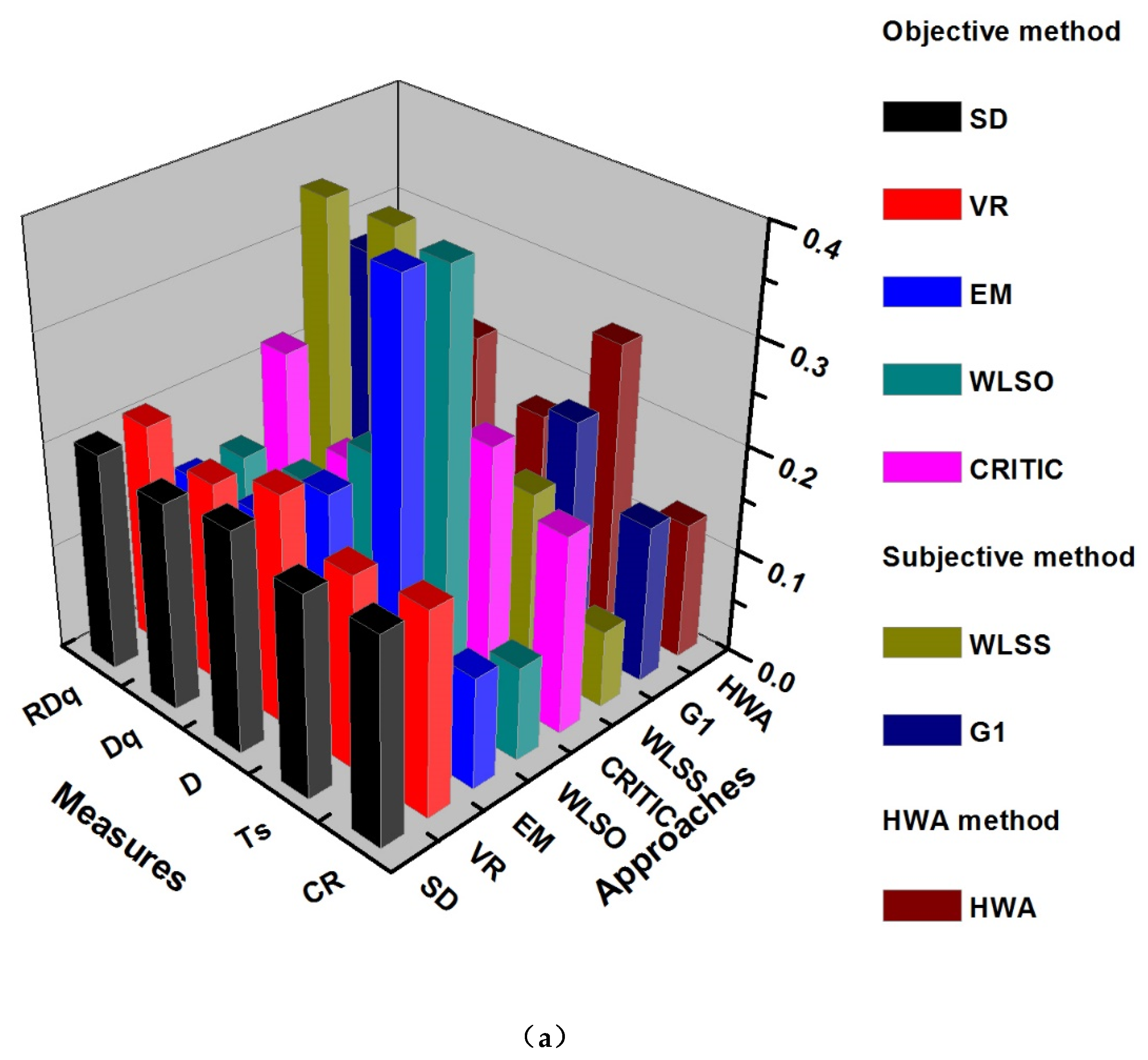
Single weighting approaches (seven approaches including the SD, VR, EM, WLSO, CRITIC, WLSS and G1 approaches) and the assembly of approaches using HWA algorithm (Figure 4a) are applied for weight calculation. Weights by objective weighting approaches (WLSO, SD, VR, EM, and CRITIC) can be directly calculated using Equations (7)–(11).

Regarding the G1 rules (listed in Table 2b), it is assumed to follow the principle that: expectation is slightly more important (1.2) than band-width; band-width is slightly more important (assign a value 1.3) than coverage; coverage is more important (1.4) than deviation amplitude; and deviation amplitude is slightly more important (assign a value 1.3) than symmetry. Relative measures are slightly more important (assign a value 1.1) than common ones. Therefore, the G1 weights are achieved as shown in

Table 7. Weights by G1 approach assessed according to the G1 relative importance standard.

	CR	B	RB	S	Ts	D	RD	Dq	RDq	NSCE
G1 weights	0.085	0.110	0.121	0.042	0.042	0.055	0.061	0.146	0.160	0.176

. The weights of contributing measures (Table 6c) picked out from Table 7 are exactly the G1 weights being normalized (shown in Figure 4a). As for the WLSS method, the relative importance follows the same order as the G1 approach but is assessed according to AHP rules in Table 2a. The subjective matrix of WLSS for the measures (CR, RB, D, Dq and RDq) is therefore assessed to be:

$$A=\left[\begin{array}{ccccc}1& 3& 2& 1/6& 1/6\\ 1/3& 1& 1/2& 1/9& 1/9\\ 1/2& 2& 1& 1/6& 1/6\\ 6& 9& 6& 1& 1\\ 6& 9& 6& 1& 1\end{array}\right]$$

The weights by all approaches are displayed in Figure 4a. If not otherwise specified, the HWA approach refers to the assembly of all seven weighting approaches. It can be seen that SD and VR methods tend to generate even weights, while EM and WLSO generally obtain the most significant weights (about 0.4) for measure Ts. On the other hand, Ts by subjective approaches (WLSS and G1) are assigned values less than 0.4, and the measures presenting the expectation (Dq and RDq) are assigned with the large weights. The weights by HWA are neither too large nor too small, which range from 0.1 to 0.26.

• Index Construction

The composite measure CUI characterizing the uncertainty interval generated by the GLUE method at different thresholds is constructed:

$$CUI=w_1\times CR+w_2\times Ts+w_3\times D+w_4\times Dq+w_5\times RQq$$

The CUIs weighted by different approaches are plotted in Figure 4b. Thresholds at horizontal axis are cut-off thresholds in GLUE. It shows that different approaches generate CUI curves with different patterns. The CUIs by subjective approaches (WLSS and G1) peak at Threshold = 0.4 while by objective approaches (SD, VR, EM, WLSO and CRITIC) peak at Threshold = 0, 0.3 or 0.4. The CUIs by HWA tend to obtain a balanced changing behavior, combining the subjective and objective ones. A proper threshold for GLUE can be obtained based on CUI. Larger CUI corresponds to a more proper cut-off threshold. HWA CUIs at a cut-off threshold between 0.3 and 0.4 are higher than that at other thresholds, therefore a cut-off threshold between 0.3 and 0.4 is proper in GLUE in this case.

The upper and lower boundaries of CUIs weighted by HWA are shown in Figure 4b. The boundaries of shadows generally show similar variation patterns with HWA CUIs (denoted as red point line). With the availability of additional subjective or statistical information (namely the incorporation of new weighing approaches into the HWA approach), the ranges of shadows are rapidly reduced. The ranges of Area5 are thinner than that of Area3. The shadow area turns into the red point line of HWA CUIs when all weighting approaches are incorporated.

On the other hand, the shadow area could also characterize the sensitivity of weight assignments (or weighting approaches) to threshold. Large bandwidth implies a significant sensitivity of the selection of weighting approaches. In this case, large bandwidth could be found at the end of high and low thresholds while a slight narrowing occurs in the low threshold section.

3.2.2. Comparisons of Different Uncertainty Analysis Approaches (Case 2)

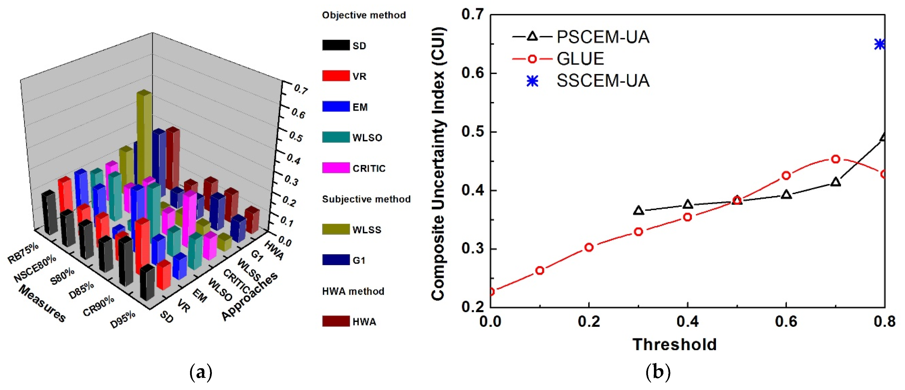
The number of events and measures increase when considering both the confidence levels and uncertainty analysis approaches, further complicating the decision matrix. The confidence levels of 95%, 90%, 85%, 80% and 75%, each level with 10 measures (Table 5), are involved in this case study, leading to a total of 50 measures. The number of contributing measures is quickly reduced to six through conducting the measure identification approach proposed in Section 2.1. D of 95% level, CR of 90% level, D of 85% level, S of 80% level, NSCE of 80% level and RB of 75% level are picked out. The six contributing measures are weighted using different approaches (Figure 5a). The CUIs weighted by the HWA approach using different uncertainty analysis approaches (GLUE, PSCEM and SSCEM-UA) are plotted in Figure 5b.

In Figure 5a, SD and VR methods yield even weights for all measures while subjective methods (WLSS and G1) give the largest weights (>0.35) to an NSCE of 80% level. The weights by HWA method range from 0.05 to 0.3, which is a balance amongst all weighting methods. Figure 5b shows the CUI values using GLUE and PSCEM-UA at different thresholds and SSCEM-UA without threshold. The CUI by the GLUE method increases at low and middle thresholds, peaks at 0.7, and decreases when threshold > 0.7. The CUI by PSCEM-UA method increases slightly when the threshold changes from 0.3 to 0.6 while sharply when threshold > 0.6. GLUE performs better than PSCEM-UA when the threshold is 0.6 and 0.7, whereas it performs worse when the threshold is less than 0.5 or larger than 0.7. It can be noted that CUI by SSCEM-UA method has only one value (0.65) in Figure 5b. The reason is that the method is conducted without pre-setting a threshold.

4. Discussion

Theoretically, an ideal uncertainty interval of simulation should be characterized by the thinnest band-width, largest coverage ratio, smallest deviation amplitude, best symmetry, and good agreement of expectations with observations. A single measure, therefore, cannot describe the uncertainty interval adequately. However, joint analysis for multiple measures always bring conflicts. Figure 3 shows that larger cut-off thresholds always correspond to a smaller band-width but a lower coverage ratio and symmetry, which is consistent with the results by Xiong et al. [20]. An individual measure could hardly act as the reference to distinguish which approach or threshold is better. A suitable cut-off threshold should balance different properties of the interval, which is called a trade-off among the uncertainty measures. The construction of the CUI in this work is an attempt to solve this problem.

It is found in Table 1 that some measures are used to describe a similar property of uncertainty interval, which may lead to information overlap. Therefore, a step of selecting behavioral measures is developed in Section 2.1 where highly correlated measures are excluded. Case 1 selected five behavioral measures amongst 10 measures and case 2 selected 6 amongst 50. The correlation coefficients between each two of the behavioral measures are low, successfully reducing information overlap. On the other hand, the measure identification approach is especially practical and convenient when encountering the occasion of an extremely large measure number where artificial identification is impossible (e.g., case 2 has 50 measures).

In the weight assignment step, case studies show that the HWA approach leads to a balance of each weight in terms of the fact that no too large or small weight could be observed (Figure 4). It could be explained by the hierarchical assembling procedure of the HWA method. Firstly, the multiplying and then extracting procedure (namely intra-class integration) effectively weakens the strengthening measures of some approaches and strengthens the weak measures of other approaches. Secondly, the mixing of both subjective and objective information supported by the difference coefficients (namely inter-class integration) could also fix the weight into a more balanced value.

The weighting approaches focus on different features of the information matrix, leading to diverse weights and different CUIs (Figure 4b). The influence from subjective weight assignation may be positive or negative, which is unavoidable. The HWA is not aiming at avoiding the influence from weight, but merging the features of different weighting approaches, so as to obtain a set of reasonable weights. Through a hierarchical ensemble of different weighting approaches, which extract different parts of information from the subjective and objective matrix, the HWA method could essentially characterize multiple properties of the information matrix. In this way, it is more synthetic and progressive theoretically. Moreover, the changing behaviors of shadow areas in Figure 4b suggest that the shape of HWA CUIs is not yielded by accident but the corollary induced by the synthetic of massive subjective and statistical information.

Figure 4b in case 1 shows that HWA CUIs at a cut-off threshold between 0.3 and 0.4 are higher than that at other thresholds. It indicates that the confidence interval at a threshold between 0.3 and 0.4 is more qualified. Therefore, a threshold between 0.3 and 0.4 can be per-set in the GLUE approach for case 1. Figure 5b in case 2 shows that CUI values by SSCEM-UA approach is larger than those by GLUE and PSCEM-UA approaches. It indicates a better assessment of the uncertainty intervals by SSCEM-UA, which could theoretically explain why most experts subjectively prefer standard Bayesian approaches to the pseudo-Bayesian approaches or GLUE approach [69,70]. On the other hand, the performances of GLUE and PSCEM-UA methods depends on the value of cut-off threshold, as GLUE is superior to PSCEM-UA at a threshold of 0.6 and 0.7 while inferior at other thresholds. The two cases indicate that CUI could serve as a criterion for identifying which cut-off threshold or uncertainty analysis method is better, providing a promising insight for similar uncertainty analysis of other statistical or environmental modeling.

Regardless of the kinds of uncertainty or uncertainty analysis approaches, the framework is able to be derived as long as the uncertainty interval is provided. Output of the framework is a composite index, which has a comparable form that can be used for the performance comparison of different uncertainty analysis approaches, the identification of thresholds in GLUE and PSCEM-UA method and so on.

5. Conclusions

A series of uncertainty measures or indices are generally used to describe the prediction bound and serve as the criterion for comparing the uncertainty intervals generated from different assessment approaches. However, an individual measure just represents part of the properties of the interval. Joint analysis using a range of measures does help to better represent the properties, but generally suffers an unavoidable conflict amongst measures. Hence, it is urgently needed to construct a composite measure for describing complex properties of the uncertainty interval and serving as criterion for the comparison of uncertainty intervals. In this work, the CUI is a composite measure that can address the above problem.

The CUI is constructed through a framework that includes measure identification, weight assignment and index construction. In the weight assignment part, a hierarchical weight assembly (HWA) method incorporating both the intra-class and inter-class weights is developed, which is conducted based on various properties of uncertainty measures and weighting methods. The framework and CUI are demonstrated by two case studies. In case 1, the weights by HWA are neither too large nor too small, which are a set of balanced values that can comprehensively merge the merits of different measures. The HWA approach is superior to other single weighting approaches both practically and theoretically. On the other hand, CUI can be used to identify proper values of cut-off thresholds in the GLUE approach. CUIs by HWA show a balanced changing behavior combining the subjective and objective ones. Proper cut-off thresholds ranging from 0.3 to 0.4 are recommended in case 1. In case 2, different uncertainty analysis approaches are compared according to CUIs. GLUE performs better than PSCEM-UA when the threshold is 0.6 and 0.7, whereas it is worse when the threshold is less than 0.5 or larger than 0.7. Besides, SSCEM-UA performs better than GLUE and PSCUM-UA.

Case studies reveal that CUI is a competitive uncertainty measure. Notwithstanding the framework and the fact that CUI are only examined in an uncertainty assessment for hydrological simulation by XAJ model in this work, it has a wide application potential in uncertainty assessment for simulation by a variety of physical-based hydrological models, stochastic hydrological models, hydraulic models, and environmental models. This work provides a novel and beneficial scientific way to quantitatively assess the complex behaviors of uncertainty. Nevertheless, there are some shortcomings, such as the form of weight assembly and the application of CUI in uncertainty assessment of other kinds, which will be further studied in our future work.

References

- Guzman, J.A.; Shirmohammadi, A.; Sadeghi, A.M.; Wang, X.; Chu, M.L.; Jha, M.K.; Parajuli, P.B.; Daren Harmel, R.; Khare, Y.P.; Hernandez, J.E. Uncertainty Considerations in Calibration and Validation of Hydrologic and Water Quality Models. Trans. ASABE 2015, 58, 1745–1762. [Google Scholar] [CrossRef] [Green Version]
- Wang, X.; Yang, T.; Yong, B.; Krysanova, V.; Shi, P.; Li, Z.; Zhou, X. Impacts of climate change on flow regime and sequential threats to riverine ecosystem in the source region of the Yellow River. Environ. Earth Sci. 2018, 77, 465. [Google Scholar] [CrossRef]
- Cui, T.; Yang, T.; Xu, C.-Y.; Shao, Q.; Wang, X.; Li, Z. Assessment of the impact of climate change on flow regime at multiple temporal scales and potential ecological implications in an alpine river. Stoch. Environ. Res. Risk Assess. 2018, 32, 1849–1866. [Google Scholar] [CrossRef]
- Kumar, A.; Yang, T.; Sharma, M.P. Long-term prediction of greenhouse gas risk to the Chinese hydropower reservoirs. Sci. Total Environ. 2019, 646, 300–308. [Google Scholar] [CrossRef] [PubMed]
- Huang, C.-S.; Yang, T.; Yeh, H.-D. Review of analytical models to stream depletion induced by pumping: Guide to model selection. J. Hydrol. 2018, 561, 277–285. [Google Scholar] [CrossRef]
- Daren Harmel, R.; Smith, P.K. Consideration of measurement uncertainty in the evaluation of goodness-of-fit in hydrologic and water quality modeling. J. Hydrol. 2007, 337, 326–336. [Google Scholar] [CrossRef]
- Yen, H.; Wang, X.; Fontane, D.G.; Harmel, R.D.; Arabi, M. A framework for propagation of uncertainty contributed by parameterization, input data, model structure, and calibration/validation data in watershed modeling. Environ. Model. Softw. 2014, 54, 211–221. [Google Scholar] [CrossRef]
- Abbaspour, K.C.; Vaghefi, S.A.; Srinivasan, R. A Guideline for Successful Calibration and Uncertainty Analysis for Soil and Water Assessment: A Review of Papers from the 2016 International SWAT Conference. Water Resour. Manag. 2018, 10, 6. [Google Scholar] [CrossRef]
- Ren, W.; Yang, T.; Shi, P.; Xu, C.-Y.; Zhang, K.; Zhou, X.; Shao, Q.; Ciais, P. A probabilistic method for streamflow projection and associated uncertainty analysis in a data sparse alpine region. Glob. Planet. Chang. 2018, 165, 100–113. [Google Scholar] [CrossRef]
- Yang, T.; Cui, T.; Xu, C.-Y.; Ciais, P.; Shi, P. Development of a new IHA method for impact assessment of climate change on flow regime. Glob. Planet. Chang. 2017, 156, 68–79. [Google Scholar] [CrossRef]
- Wang, X.; Yang, T.; Wortmann, M.; Shi, P.; Hattermann, F.; Lobanova, A.; Aich, V. Analysis of multi-dimensional hydrological alterations under climate change for four major river basins in different climate zones. Clim. Chang. 2017, 141, 483–498. [Google Scholar] [CrossRef]
- Singh, V.P. Computer Models of Watershed Hydrology; Water Resources Publications, LLC: Highlands Ranch, CO, USA, 1995. [Google Scholar]
- Beven, K.; Binley, A. The future of distributed models: Model calibration and uncertainty prediction. Hydrol. Process. 1992, 6, 279–298. [Google Scholar] [CrossRef]
- Muleta, M.K.; Nicklow, J.W. Sensitivity and uncertainty analysis coupled with automatic calibration for a distributed watershed model. J. Hydrol. 2005, 306, 127–145. [Google Scholar] [CrossRef]
- Van Griensven, A.; Meixner, T.; Grunwald, S.; Bishop, T.; Diluzio, M.; Srinivasan, R. A global sensitivity analysis tool for the parameters of multi-variable catchment models. J. Hydrol. 2006, 324, 10–23. [Google Scholar] [CrossRef]
- Yang, J.; Reichert, P.; Abbaspour, K.C.; Xia, J.; Yang, H. Comparing uncertainty analysis techniques for a SWAT application to the Chaohe Basin in China. J. Hydrol. 2008, 358, 1–23. [Google Scholar] [CrossRef]
- Hoeting, J.A.; Madigan, D.; Raftery, A.E.; Volinsky, C.T. Bayesian Model Averaging: A Tutorial. Stat. Sci. 1999, 14, 382–401. [Google Scholar]
- Ajami, N.K.; Duan, Q.; Sorooshian, S. An integrated hydrologic Bayesian multimodel combination framework: Confronting input, parameter, and model structural uncertainty in hydrologic prediction. Water Resour. Res. 2007, 43. [Google Scholar] [CrossRef] [Green Version]
- Zhou, R.; Li, Y.; Lu, D.; Liu, H.; Zhou, H. An optimization based sampling approach for multiple metrics uncertainty analysis using generalized likelihood uncertainty estimation. J. Hydrol. 2016, 540, 274–286. [Google Scholar] [CrossRef]
- Xiong, L.; Wan, M.I.N.; Wei, X.; O’Connor, K.M. Indices for assessing the prediction bounds of hydrological models and application by generalised likelihood uncertainty estimation/Indices pour évaluer les bornes de prévision de modèles hydrologiques et mise en œuvre pour une estimation d’incertitude par vraisemblance généralisée. Hydrol. Sci. J. 2009, 54, 852–871. [Google Scholar] [CrossRef]
- Melching, C.S.; Singh, V.P. Reliability Estimation, Computer Models of Watershed Hydrology; Water Resources Publications: Highlands Ranch, CO, USA, 1995. [Google Scholar]
- Legates, D.R.; McCabe, G.J., Jr. Evaluating the use of “goodness-of-fit” Measures in hydrologic and hydroclimatic model validation. Water Resour. Res. 1999, 35, 233–241. [Google Scholar] [CrossRef] [Green Version]
- Montanari, A. Large sample behaviors of the generalized likelihood uncertainty estimation (GLUE) in assessing the uncertainty of rainfall-runoff simulations. Water Resour. Res. 2005, 41. [Google Scholar] [CrossRef] [Green Version]
- Jin, X.; Xu, C.-Y.; Zhang, Q.; Singh, V.P. Parameter and modeling uncertainty simulated by GLUE and a formal Bayesian method for a conceptual hydrological model. J. Hydrol. 2010, 383, 147–155. [Google Scholar] [CrossRef]
- Olsson, J.; Lindström, G. Evaluation and calibration of operational hydrological ensemble forecasts in Sweden. J. Hydrol. 2008, 350, 14–24. [Google Scholar] [CrossRef]
- Blasone, R.-S.; Madsen, H.; Rosbjerg, D. Uncertainty assessment of integrated distributed hydrological models using GLUE with Markov chain Monte Carlo sampling. J. Hydrol. 2008, 353, 18–32. [Google Scholar] [CrossRef] [Green Version]
- Chen, X.; Yang, T.; Wang, X.; Xu, C.-Y.; Yu, Z. Uncertainty Intercomparison of Different Hydrological Models in Simulating Extreme Flows. Water Resour. Manag. 2013, 27, 1393–1409. [Google Scholar] [CrossRef]
- Xiong, L.; O’Connor, K.M. An empirical method to improve the prediction limits of the GLUE methodology in rainfall–runoff modeling. J. Hydrol. 2008, 349, 115–124. [Google Scholar] [CrossRef]
- Dong, L.; Xiong, L.; Zheng, Y. Uncertainty analysis of coupling multiple hydrologic models and multiple objective functions in Han River, China. Water Sci. Technol. 2013, 68, 506–513. [Google Scholar] [CrossRef]
- Si, W.; Bao, W.; Gupta, H.V. Updating real-time flood forecasts via the dynamic system response curve method. Water Resour. Res. 2015, 51, 5128–5144. [Google Scholar] [CrossRef] [Green Version]
- Chen, T.-Y.; Li, C.-H. Determining objective weights with intuitionistic fuzzy entropy measures: A comparative analysis. Inf. Sci. 2010, 180, 4207–4222. [Google Scholar] [CrossRef]
- Choo, E.U.; Wedley, W.C. Optimal Criterion Weights in Repetitive Multicriteria Decision-Making. J. Oper. Res. Soc. 1985, 36, 983–992. [Google Scholar] [CrossRef]
- Cruz, J.M. The impact of corporate social responsibility in supply chain management: Multicriteria decision-making approach. Decis. Support Syst. 2009, 48, 224–236. [Google Scholar] [CrossRef]
- Rao, R. A note on “An alternative multiple attribute decision making methodology for solving optimal facility layout design selection problems”. Int. J. Ind. Eng. Comput. 2012, 3, 519–524. [Google Scholar]
- Xu, Z. Attribute weights determination models for consensus maximization in multiple attribute group decision-making. Int. J. Gen. Syst. 2011, 40, 755–774. [Google Scholar] [CrossRef]
- Rao, R.V.; Davim, J.P. A decision-making framework model for material selection using a combined multiple attribute decision-making method. Int. J. Adv. Manuf. Technol. 2008, 35, 751–760. [Google Scholar] [CrossRef]
- Qin, Y.; Kavetski, D.; Kuczera, G. A Robust Gauss-Newton Algorithm for the Optimization of Hydrological Models: From Standard Gauss-Newton to Robust Gauss-Newton. Water Resour. Res. 2018, 54, 9655–9683. [Google Scholar] [CrossRef]
- Qin, Y.; Kavetski, D.; Kuczera, G. A Robust Gauss-Newton Algorithm for the Optimization of Hydrological Models: Benchmarking Against Industry-Standard Algorithms. Water Resour. Res. 2018, 54, 9637–9654. [Google Scholar] [CrossRef]
- Md Saad, R.; Ahmad, M.Z.; Abu, M.S.; Jusoh, M.S. Hamming Distance Method with Subjective and Objective Weights for Personnel Selection. Sci. World J. 2014, 2014, 9. [Google Scholar] [CrossRef] [PubMed]
- Dadelo, S.; Turskis, Z.; Zavadskas, E.K.; Dadeliene, R. Multi-criteria assessment and ranking system of sport team formation based on objective-measured values of criteria set. Expert Syst. Appl. 2014, 41, 6106–6113. [Google Scholar] [CrossRef]
- Okoli, C.; Pawlowski, S.D. The Delphi method as a research tool: An example, design considerations and applications. Inf. Manag. 2004, 42, 15–29. [Google Scholar] [CrossRef]
- Saaty, T.L. A scaling method for priorities in hierarchical structures. J. Math. Psychol. 1977, 15, 234–281. [Google Scholar] [CrossRef]
- Saaty, T.L.; Saaty, T.L. Fundamentals of Decision Making and Priority Theory with the Analytic Hierarchy Process; RWS Publications: Pittsburgh, PA, USA, 2006. [Google Scholar]
- Bryson, N. A Goal Programming Method for Generating Priority Vectors. J. Oper. Res. Soc. 1995, 46, 641–648. [Google Scholar] [CrossRef]
- Bryson, N.; Joseph, A. Generating consensus priority point vectors: a logarithmic goal programming approach. Comput. Oper. Res. 1999, 26, 637–643. [Google Scholar] [CrossRef]
- Harte, J.M.; Koele, P.; van Engelenburg, G. Estimation of attribute weights in a multiattribute choice situation. Acta Psychol. 1996, 93, 37–55. [Google Scholar] [CrossRef]
- Herrera, F.; Martínez, L.; Sánchez, P.J. Managing non-homogeneous information in group decision making. Eur. J. Oper. Res. 2005, 166, 115–132. [Google Scholar] [CrossRef]
- Jahan, A.; Mustapha, F.; Sapuan, S.M.; Ismail, M.Y.; Bahraminasab, M. A framework for weighting of criteria in ranking stage of material selection process. Int. J. Adv. Manuf. Technol. 2012, 58, 411–420. [Google Scholar] [CrossRef]
- Wang, W.-D.; Guo, J.; Fang, L.-G.; Chang, X.-S. A subjective and objective integrated weighting method for landslides susceptibility mapping based on GIS. Environ. Earth Sci. 2012, 65, 1705–1714. [Google Scholar] [CrossRef]
- Nasiri, F.; Huang, G. A fuzzy decision aid model for environmental performance assessment in waste recycling. Environ. Model. Softw. 2008, 23, 677–689. [Google Scholar] [CrossRef]
- Pradhan, M.K. Optimization of MRR, TWR and surface roughness of EDMed D2 Steel using an integrated approach of RSM, GRA and Entropy measutement method. In Proceedings of the 2013 International Conference on Energy Efficient Technologies for Sustainability, Nagercoil, India, 10–12 April 2013; pp. 865–869. [Google Scholar]
- Pakkar, M.S. An integrated approach based on DEA and AHP. Comput. Manag. Sci. 2015, 12, 153–169. [Google Scholar] [CrossRef]
- Guo, Y. Theory, Algorithm and Application of Comprehensive Assessment; Science Press: Beijing, China, 2007. [Google Scholar]
- Zheng, H. Multi-Sensor Target Recognition Using VIKOR Combined with G1 Method. Appl. Mech. Mater. 2015, 707, 321–324. [Google Scholar] [CrossRef]
- Xie, X.J. Research on Material Selection with Multi-Attribute Decision Method and G1 Method. Adv. Mater. Res. 2014, 952, 20–24. [Google Scholar] [CrossRef]
- Chu, A.T.W.; Kalaba, R.E.; Spingarn, K. A comparison of two methods for determining the weights of belonging to fuzzy sets. J. Optim. Theory Appl. 1979, 27, 531–538. [Google Scholar] [CrossRef]
- Ma, J.; Fan, Z.-P.; Huang, L.-H. A subjective and objective integrated approach to determine attribute weights. Eur. J. Oper. Res. 1999, 112, 397–404. [Google Scholar] [CrossRef] [Green Version]
- Zou, Z.-h.; Yun, Y.; Sun, J.-n. Entropy method for determination of weight of evaluating indicators in fuzzy synthetic evaluation for water quality assessment. J. Environ. Sci. 2006, 18, 1020–1023. [Google Scholar] [CrossRef]
- Diakoulaki, D.; Mavrotas, G.; Papayannakis, L. Determining objective weights in multiple criteria problems: The critic method. Comput. Oper. Res. 1995, 22, 763–770. [Google Scholar] [CrossRef]
- Shannon, C.E. Prediction and Entropy of Printed English. Bell Syst. Tech. J. 1951, 30, 50–64. [Google Scholar] [CrossRef]
- Li, Z.; Yang, T.; Huang, C.-S.; Xu, C.-Y.; Shao, Q.; Shi, P.; Wang, X.; Cui, T. An improved approach for water quality evaluation: TOPSIS-based informative weighting and ranking (TIWR) approach. Ecol. Indic. 2018, 89, 356–364. [Google Scholar] [CrossRef]
- French, S. Multi-Objective Decision Making: Based on the Proceedings of a Conference on Multi-Objective Decision Making; Academic Press: London, UK; New York, NY, USA, 1983. [Google Scholar]
- Zhao, R.-J. The Xinanjiang model applied in China. J. Hydrol. 1992, 135, 371–381. [Google Scholar] [CrossRef]
- Shi, P.; Yang, T.; Xu, C.-Y.; Yong, B.; Shao, Q.; Li, Z.; Wang, X.; Zhou, X.; Li, S. How do the multiple large-scale climate oscillations trigger extreme precipitation? Glob. Planet. Chang. 2017, 157, 48–58. [Google Scholar] [CrossRef]
- Zhang, D.; Zhang, L.; Guan, Y.; Chen, X.; Chen, X. Sensitivity analysis of Xinanjiang rainfall–runoff model parameters: A case study in Lianghui, Zhejiang province, China. Hydrol. Res. 2012, 43, 123–134. [Google Scholar] [CrossRef]
- Beven, K. Changing ideas in hydrology—The case of physically-based models. J. Hydrol. 1989, 105, 157–172. [Google Scholar] [CrossRef]
- Beven, K. Prophecy, reality and uncertainty in distributed hydrological modelling. Adv. Water Resour. 1993, 16, 41–51. [Google Scholar] [CrossRef]
- Choi, H.T.; Beven, K. Multi-period and multi-criteria model conditioning to reduce prediction uncertainty in an application of TOPMODEL within the GLUE framework. J. Hydrol. 2007, 332, 316–336. [Google Scholar] [CrossRef]
- Vrugt, J.A.; ter Braak, C.J.F.; Gupta, H.V.; Robinson, B.A. Equifinality of formal (DREAM) and informal (GLUE) Bayesian approaches in hydrologic modeling? Stoch. Environ. Res. Risk Assess. 2009, 23, 1011–1026. [Google Scholar] [CrossRef]
- Li, L.; Xu, C.-Y. The comparison of sensitivity analysis of hydrological uncertainty estimates by GLUE and Bayesian method under the impact of precipitation errors. Stoch. Environ. Res. Risk Assess. 2014, 28, 491–504. [Google Scholar] [CrossRef]
Figure 1.
General methodology.
Figure 2.
Map of the study area controlled by Lushi hydrological station.
Figure 3.
Time-continuous 95% confidence intervals simulated respectively by (a) GLUE, (b) PSCEM-UA and (c) SSCEM-UA approaches at threshold = 0.5 and 0.8 during the period 1983–1987.
Figure 4.
(a) Inter-comparisons of weights calculated by different weighting methods; (b) CUIs by weighting different methods at different thresholds of GLUE. Note: the shadow areas denote the CUIs weighted by the HWA approach assembling any three (the shallow one refers to Area 3) or five (the dark one refers to Area 5) single weighting approaches.
Figure 5.
(a) Bar plots of weights assigned by different weighting approaches; (b) CUIs by HWA weighting approach using different uncertainty analysis approaches (GLUE and PSCEM-UA at different thresholds, and SSCEM-UA without threshold).